| Issue |
A&A
Volume 681, January 2024
|
|
|---|---|---|
| Article Number | A11 | |
| Number of page(s) | 25 | |
| Section | Stellar structure and evolution | |
| DOI | https://doi.org/10.1051/0004-6361/202346715 | |
| Published online | 05 January 2024 | |
Spectropolarimetry of Type II supernovae
II. Intrinsic supernova polarization and its relation to photometric and spectroscopic properties
1
Department of Physics and Astronomy, University of Turku, Vesilinnantie 5, 20014 Turku, Finland
e-mail: This email address is being protected from spambots. You need JavaScript enabled to view it.
2
Aalto University Metsähovi Radio Observatory, Metsähovintie 114, 02540 Kylmälä, Finland
3
Aalto University Department of Electronics and Nanoengineering, PO Box 15500 00076 Aalto, Finland
4
European Southern Observatory, Karl-Schwarzschild-Str. 2, 85748 Garching b. München, Germany
5
Gemini Observatory/NSF’s NOIRLab, Casilla 603, La Serena, Chile
6
School of Sciences, European University Cyprus, Diogenes street, Engomi, 1516 Nicosia, Cyprus
7
Finnish Centre for Astronomy with ESO (FINCA), University of Turku, Vesilinnantie 5, 20014 Turku, Finland
8
Department of Physics and Earth Science, University of Ferrara, Via Saragat 1, 44122 Ferrara, Italy
9
INFN, Sezione di Ferrara, Via Saragat 1, 44122 Ferrara, Italy
10
INAF, Osservatorio Astronomico d’Abruzzo, Via Mentore Maggini snc, 64100 Teramo, Italy
11
Departamento de Ciencias Fisicas, Universidad Andres Bello, Avda. Republica 252, Santiago, Chile
Received:
20
April
2023
Accepted:
1
October
2023
Abstract
The explosion processes of supernovae (SNe) are imprinted in their explosion geometries. The recent discovery of several highly aspherical core-collapse SNe is significant, and studying these is regarded as being crucial in order to understand the underlying explosion mechanism. Here, we study the intrinsic polarization of 15 hydrogen-rich core-collapse SNe and explore the relation between polarization and the photometric and spectroscopic properties of these objects. Our sample shows diverse properties of the continuum polarization. Most SNe show a low degree of polarization at early phases but a sudden rise to ∼1% at certain points during the photospheric phase followed by a slow decline during the tail phase, with a constant polarization angle. The variation in the timing of peak polarization values implies diversity in the explosion geometry: some SNe have aspherical structures only in their helium cores, while in other SNe such structures reach out to a significant part of the outer hydrogen envelope with a common axis from the helium core to the hydrogen envelope. Other SNe show high polarization from early phases and a change in polarization angle around the middle of the photospheric phase. This implies that the ejecta are significantly aspherical out to the outermost layer and have multi-directional aspherical structures. Exceptionally, the Type IIL SN 2017ahn shows low polarization at both the photospheric and tail phases. Our results show that the timing of the polarization rise in Type IIP SNe is likely correlated with their brightness, velocity, and the amount of radioactive Ni produced: brighter SNe with faster ejecta velocity and a larger 56Ni mass have more extended aspherical explosion geometries. In particular, there is a clear correlation between the timing of the polarization rise and the explosion energy; that is, the explosion asphericity is proportional to the explosion energy. This implies that the development of a global aspherical structure, such as a jet, might be the key for the realisation of an energetic SN in the mechanism of SN explosions.
Key words: supernovae: general / techniques: polarimetric
© The Authors 2024
 Open Access article, published by EDP Sciences, under the terms of the Creative Commons Attribution License (https://creativecommons.org/licenses/by/4.0), which permits unrestricted use, distribution, and reproduction in any medium, provided the original work is properly cited.
This article is published in open access under the Subscribe to Open model. This email address is being protected from spambots. You need JavaScript enabled to view it. to support open access publication.
1. Introduction
Core-collapse supernovae (CCSNe) are catastrophic explosions of massive stars at their deaths. This phenomenon is closely related to the evolution of galaxies through processes such as the chemical enrichment of galaxies and the induction of star formation. Despite significant effort, the explosion mechanism is not yet fully understood. The most promising picture is the neutrino-driven explosion, in which a star blows up due to neutrino heating from a protoneutron star (e.g., Janka et al. 2007; Janka 2012). Although some recent multidimensional simulations have been successful in launching the explosion, they are unable to reproduce some of the basic observed properties; for example, the 1051 erg of explosion energy (e.g., Buras et al. 2006; Marek & Janka 2009; Takiwaki et al. 2012; Hanke et al. 2013; Melson et al. 2015). The results of these simulations indicate that some multidimensional hydrodynamic instabilities, such as convective motion (e.g., Herant et al. 1994) and the standing-accretion-shock-instability (SASI; e.g., Foglizzo 2002; Blondin et al. 2003), might play a crucial role in producing energetic explosions, because the random movement of the ejecta gas due to the instabilities can increase the neutrino heating efficiency in the gain region. It has also been proposed that additional effects that enhance certain instabilities enable the production of realistic SN explosions, such as effects from general relativity, rotation, magnetic fields, and inhomogeneities in the progenitor core. The asymmetries resulting from instabilities in the inner core might introduce Rayleigh–Taylor (RT) instability at the C+O/He and He/H composition interfaces and create global asymmetries in the ejecta (e.g., Wongwathanarat et al. 2015).
Investigating explosion geometries of SNe can provide insights into the explosion mechanism. In particular, it is critically important to clarify the relations between explosion asphericity and SN properties, such as explosion energy, ejecta mass, and progenitor radius. The proposed explosion scenarios can be tested by comparing these relations with those from theoretical simulations. The most reliable and direct way to investigate the geometry of a spatially unresolved SN is polarimetry. For an SN with a spherically symmetric photosphere, no polarization is expected because of the cancellation of the orthogonal Stokes vectors. Therefore, the detection of a non-null continuum polarization provides direct and independent evidence for an overall asphericity.
Hydrogen-rich CCSNe (hereafter Type II SNe) are classified into two subtypes, Type IIP and IIL, based on the light-curve shapes. Type IIP SNe are the most common class of CCSNe (∼50% of all CC events; e.g., Li et al. 2011). These objects show constant optical brightness until ∼100 days post-explosion (the photospheric phase), which is followed by an exponential flux decline (the tail phase) after a sudden drop (e.g., Anderson et al. 2014; Faran et al. 2014a; Sanders et al. 2015; Valenti et al. 2016). In general, a low level of polarization (∼0.1%) has been measured during the photospheric phase, while a rapid increase in continuum polarization (∼1.0%) is seen at the beginning of the tail phase in some Type IIP SNe (e.g., Leonard et al. 2001, 2006; Chornock et al. 2010; Kumar et al. 2016). This polarimetric feature can be explained by an asymmetric helium core being revealed when the outer spherical hydrogen envelope becomes optically thin as indicated by the light curve falling off the plateau (e.g., Leonard et al. 2006). On the other hand, Dessart & Hillier (2011), based on the polarimetric calculations from axially symmetric SN ejecta artificially constructed using one-dimensional inputs from nonlocal-thermodynamic-equilibrium radiative-transfer simulations, demonstrated that the small continuum polarization during the photospheric phase can, in some cases, be reproduced by optical-depth effects irrespective of the magnitude of the asphericity of the hydrogen envelope. Although only a few Type IIP SNe have been observed in polarimetry with a sufficient temporal coverage, this high polarization is regarded as supporting evidence for the asymmetric explosions suggested by some numerical simulations (e.g., Janka 2012). Recently, Nagao et al. (2019) found an unprecedented, highly extended aspherical explosion in SN 2017gmr indicated by an early rise in polarization, hence clearly showing that asymmetries are present not only in the helium core but also in a substantial portion of the hydrogen envelope. This demonstrates the existence of an intrinsic diversity in the aspherical structure of Type IIP SN explosions.
Type IIL SNe are a relatively rare subtype of Type II SNe that show a linear decline in their brightness during the photospheric phase (e.g., Faran et al. 2014b). Very few Type IIL SNe have been observed with polarimetry. Nagao et al. (2021) reported that low polarization was observed during the entire evolution from the photospheric to the tail phases in SN 2017ahn, while SN 2013ej showed high polarization from the beginning of the photospheric phase. Based on the polarization analysis of SNe 2017ahn and 2013ej, Nagao et al. (2021) claim that there are at least two subtypes of Type IIL SNe in terms of their explosion schemes: some SNe may come from explosions that are different from those leading to Type IIP SNe (a spherical explosion; e.g., SN 2017ahn) and others can come from similar explosions (an aspherical explosion; e.g., SN 2013ej).
In this study, we investigate the polarimetric properties of 15 Type II SNe using unpublished and published spectropolarimetric data obtained with the Very Large Telescope (VLT) and other telescopes. We have divided our analysis into two papers. In Nagao et al. (2023; hereafter Paper I), we present the full description of our SN sample, the observations, data reduction techniques, and our method to estimate the interstellar polarization (ISP). We also investigate the properties of the ISP components of 11 well-observed SNe from our sample in Paper I. Here, we discuss the properties of the intrinsic SN polarization of 15 SNe from our SN sample, their photometric and spectroscopic properties, and the relations between these properties, with the aim of exploring possible relations between the explosion asphericity and the explosion physics. Throughout this work, Type IIP and IIL are distinguished from one another based on their light-curve shapes, with this latter being quantified by the value of the decline rate during the photospheric phase (sp; see Sect. 3.1). In the following sections, we show the polarimetric (Sect. 2), photometric, and spectroscopic (Sect. 3) properties of our sample. In Sect. 4, we discuss relations between the polarimetric properties and the other observational properties of the SNe. Our conclusions are finally presented in Sect. 5.
2. Properties of intrinsic SN polarization
In this section, we discuss the continuum polarization in the intrinsic SN polarization, which is derived by subtracting the ISP component from the observed polarization spectrum. The full description of our SN sample, the observations, the data reduction techniques, and the method to estimate the interstellar polarization are presented in Paper I. As for the VLT sample, we calculate the continuum polarization in the same way as Chornock et al. (2010), Nagao et al. (2019, 2021). We independently take the averages of the ordinary fluxes and the extraordinary fluxes of the reduced polarization spectra (see Sect. 3.1 in Paper I) within the wavelength ranges 6800–7200 Å and 7820–8140 Å towards each half-wave retarder-plate angle. From these averaged fluxes of the ordinary and extraordinary beams, we calculate the Stokes Q and U values and thereby the polarization degree and angle for the continuum polarization using the standard methods described in Patat & Romaniello (2006). The polarization bias in the polarization degrees was removed according to the standard procedure in Wang et al. (1997). The derived values are discussed in Sect. 2.1 and shown in Figs. 1–11. It is noted that, for SNe 1999em, 2004dj, 2006ov, and 2007aa, we instead adopted the derived values for the ISP and the intrinsic SN polarization from the literature (Leonard et al. 2001, 2006; Chornock et al. 2010). As the continuum polarization of SN 1999em, we adopted the V-band polarization values that were measured by calculating the debiased, flux-weighted averages of q and u over the intervals 6050–6950 Å for the first epoch and 5050–5950 Å for the other epochs (Leonard et al. 2001). For SN 2004dj, we adopted the continuum polarization values that were derived as the median values of the Stokes parameters over the interval 6800–8200 Å (Leonard et al. 2006). The continuum polarization values for SNe 2006ov and 2007aa were derived in the same way as in the present paper for the VLT sample.
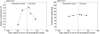 |
Fig. 1. Polarization degree and angle of the continuum polarization in SN 2017gmr. |
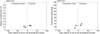 |
Fig. 2. Polarization degree and angle of the continuum polarization in SN 2017ahn. |
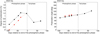 |
Fig. 3. Polarization degree and angle of the continuum polarization in SN 2013ej. The explosion component is shown in red. |
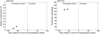 |
Fig. 4. Polarization degree and angle of the continuum polarization in SN 2012ec. |
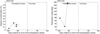 |
Fig. 5. Polarization degree and angle of the continuum polarization in SN 2012dh. |
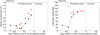 |
Fig. 6. Polarization degree and angle of the continuum polarization in SN 2012aw. The aspherical explosion component is shown in red. |
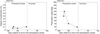 |
Fig. 7. Polarization degree and angle of the continuum polarization in SN 2010hv. |
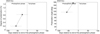 |
Fig. 8. Polarization degree and angle of the continuum polarization in SN 2010co. |
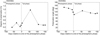 |
Fig. 9. Polarization degree and angle of the continuum polarization in SN 2008bk. |
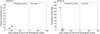 |
Fig. 10. Polarization degree and angle of the continuum polarization in SN 2001du. |
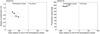 |
Fig. 11. Polarization degree and angle of the continuum polarization in SN 2001dh. |
In addition to the ISP, the continuum polarization observed in Type II SNe has two possible origins: electron scattering in an aspherical photosphere (the aspherical-photosphere origin) and dust scattering in aspherically distributed circumstellar material (CSM; the dust-scattering origin; see, e.g., Nagao et al. 2019, 2021, and references therein). In the case of the former, the polarization is wavelength independent, while in the latter, some wavelength dependence is expected (see Nagao et al. 2018, for details). As none of the polarization spectra in our sample show a clear wavelength dependence (see Figs. B.1–B.11) at any phase, we conclude that the continuum polarization of all the SNe at all the epochs in our sample originates from aspherical structures in their photosphere. Such asphericities can be created by an aspherical explosion (e.g., SN 2017gmr; Nagao et al. 2019), an ejecta interaction with aspherical CSM (e.g., SN 2013ej; Nagao et al. 2021), or other unknown processes.
2.1. Individual SNe in the VLT sample
The VLT sample consists of the following 11 SNe: SNe 2017gmr, 2017ahn, 2013ej, 2012ec, 2012dh, 2012aw, 2010hv, 2010co, 2008bk, 2001du, and 2001dh. The individual objects are discussed in the following subsections.
2.1.1. SN 2017gmr
The data for SN 2017gmr were already discussed in Nagao et al. (2019). As shown in that work, the intrinsic continuum polarization of SN 2017gmr is shown to be of a high degree (∼0.8%), with a constant angle (∼95°) from the middle of the photospheric phase to the beginning of the tail phase (see Fig. 1). This indicates that the asymmetry is not confined to the helium core but extends to a significant part of the hydrogen envelope, and that the SN has a global aspherical structure from the helium core to the hydrogen envelope; for example, a jet-like structure. As the SN did not show any features due to a strong CSM interaction (see Andrews et al. 2019), we believe the origin of this polarization to be the aspherical structure of the ejecta originating from an aspherical explosion (see also discussions in Nagao et al. 2019). In addition, as the polarization evolution in the tail phase is similar to other Type IIP SNe that are believed to be aspherical explosions (t−2 evolution, which can be interpreted as being due to geometrical dilution that reduces the optical depth of the ejecta; e.g., SN 2004dj Leonard et al. 2006), it is natural to conclude that the origin is a common feature of such objects; that is, an aspherical explosion. This conclusion is supported by the asymmetric lines seen in the nebular spectra of SN 2017gmr (e.g., Andrews et al. 2019; Utrobin et al. 2021).
2.1.2. SN 2017ahn
The data for SN 2017ahn were already presented in Nagao et al. (2021). As discussed in that paper, the continuum polarization of this object remains low from the photospheric to tail phases (Fig. 2), which implies a purely spherical explosion or a polar viewing angle of an aspherical explosion. We note that, at the first two epochs (and possibly also at the other epochs as well), the polarization might show a component in the bluer wavelengths (λ < 6000 Å) with a degree of polarization of ∼0.5% (see Fig. B.2). This might originate from some line polarization, some dust scattering component, or an incomplete ISP subtraction.
2.1.3. SN 2013ej
The data for SN 2013ej were already discussed in Nagao et al. (2021). The continuum polarization of this SN has two components with different angles, possibly consisting of an interaction component (originating from the aspherical CSM interaction) and an explosion component (arising from an aspherical explosion). Following the discussion in Nagao et al. (2021), we assume that the signal at the first epoch comes purely from the CSM interaction (P = 0.40% and θ = 78.4°). The explosion component, which is derived by subtracting the interaction component from the observed polarization, is shown in Fig. 3 and Table A.3. Hereafter, we consider only the explosion component as the continuum polarization of SN 2013ej.
2.1.4. SN 2012ec
This SN shows low polarization degrees at least until the latest observation (Phase −54.49 days; see Fig. 4). This implies that the shape of the photosphere is likely close to spherical, at least until this epoch.
2.1.5. SN 2012dh
SN 2012dh shows a relatively low polarization level (P < 0.3%) until the epoch of the last observation (phase −54.37 ± 16.40 days), with erratic polarization angles (see Fig. 5). This implies that the shape of the photosphere is quite spherical, at least until this phase. Here, the large error bars in the phases originate from the large uncertainty on the end of the photospheric phase.
2.1.6. SN 2012aw
The data for SN 2012aw were already discussed in Dessart et al. (2021), although these authors assumed slightly different values for the ISP (see Paper I). As in SN 2013ej, SN 2012aw has at least two components that show a change in polarization angle with time: a component with θ ∼ 35° and a component with θ ∼ 125° (see Fig. 6). The first two epochs appear to be dominated by the first component with a relatively constant polarization angle P ∼ 0.35%, while the later epochs seem to be affected by the second time-evolving component with another constant polarization angle, θ ∼ 125°. This behavior of the continuum polarization is similar to that of SN 2013ej (Nagao et al. 2021). As in this latter case, the first and second components might be due to a combination of an aspherical CSM interaction and an aspherical explosion, respectively. However, as opposed to SN 2013ej, SN 2012aw did not show strong interaction features in its photometric and spectroscopic properties at early phases. In addition, the two components are close to perpendicular, which might suggest the presence of two-component ejecta driven by a “jet” explosion (a collimated high-energy component and a canonical, bulk SN component).
Assuming the signals in the first epoch represent only one component (P ∼ 0.35% and θ = 34.8°), we derive the remaining component by subtracting this first component from the original polarization signals (see Fig. 6). This remaining component shows a relatively constant polarization angle (θ ∼ 120°) as well as a polarization rise similar to the behavior seen for SNe 2017gmr and 2013ej. We therefore assume that the remaining component is related to an aspherical explosion, as in other SNe, such as SNe 2017gmr and 2013ej. We note that the angle of the second component at the second epoch differs from those at the other epochs. This may be due to the large uncertainty originating from the subtraction of similar vectors in the Q–U plane, which we do not take into account for the error estimation of the polarization angles.
The difference in polarization angle between the first component and the explosion component is ∼90° for SN 2012aw, while it is ∼20° for SN 2013ej (see Tables A.3 and A.6). If the origin of the first component for SN 2012aw is the same as for SN 2013ej, which is supposed to come from an aspherical CSM interaction (Nagao et al. 2021), this might indicate that the orientations of the aspherical structures of the explosion and the CSM distribution are independent. In turn, this suggests that the two asphericities (the first and second polarization components) are produced by different mechanisms. Unlike SN 2013ej, SN 2012aw does not show any clear evidence for a strong CSM interaction in the light curve and spectra during the photospheric phase. Therefore, the origin of the first component may be different in the two objects. The number of SNe showing such a component is still too small to allow any firm conclusion on its nature. Hereafter, we consider only the second component (red points in Fig. 6) as the continuum polarization of SN 2012aw.
2.1.7. SN 2010hv
SN 2010hv shows low polarization degrees during most parts of the photospheric phase (see Fig. 7), although there is a large uncertainty in the phases. This implies that either most of the hydrogen envelope is quite spherical or that the viewing angle is close to polar for an aspherical structure.
2.1.8. SN 2010co
SN 2010co shows a polarization rise during the photospheric phase akin to that seen for SNe 2017gmr, 2013ej, and 2012aw. This implies that this SN also has an aspherical structure extending to the hydrogen envelope.
2.1.9. SN 2008bk
SN 2008bk shows relatively low polarization degrees during the photospheric phase, while it develops high polarization in the tail phase. It is not clear whether the timing of the polarization rise corresponds to the luminosity drop, as in the other SNe, because that part of the polarimetric evolution (occurring between our fifth and sixth epochs) is not covered by the available data. However, the general behavior is similar to that expected for the classical scenario (e.g., SN 2004dj; Leonard et al. 2006): an aspherical He core surrounded by a spherical hydrogen envelope. As the polarization degree around 60 days after the luminosity drop is high (P ∼ 1.17%) compared to that seen in the other SNe in our sample (see Fig. 12), the actual polarization peak might also be high (∼2%) just after the luminosity drop, that is, if this SN also follows the t−2 evolution. This might imply a very aspherical He core.
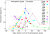 |
Fig. 12. Time evolution of the continuum polarization of our SN sample. Here, for SNe 2013ej and 2012aw, we plot the explosion components after the subtraction of the interaction components. |
2.1.10. SN 2001du
Although there are relatively few data for SN 2001du, this object shows low polarization degrees at least at the start of the photospheric phase, unlike SNe 2013ej and 2012aw. This behavior is seen in most Type II SNe.
2.1.11. SN 2001dh
The continuum polarization of SN 2001dh shows a very different behavior from that seen in all the other SNe observed so far in that it displays a component with a single polarization angle (θ ∼ 160°), which declines from a level of ∼1% during the photospheric phase. The 1% continuum polarization at the start of the photospheric phase is the highest level ever recorded among all observed Type II SNe. In addition, such a marked decline has not been observed in any other SNe. As it is difficult for an aspherical explosion to create aspherical structure in only the outermost layers, this polarization decline might be due to cancellation of polarization components by multiple aspherical structures as in SNe 2013ej and 2012aw.
2.2. Diversity in the continuum polarization
Figure 12 shows the time evolution of the continuum polarization of the SNe in our sample. All the SNe, with exception of SN 2017ahn, show relatively high degrees of polarization at some epoch (∼1%), although there is large diversity in the temporal evolution. This supports the position that an aspherical structure is a common feature in Type II SNe (e.g., Wang & Wheeler 2008).
A polarization level as large as ∼1% corresponds to an asphericity with a minimum axis ratio of 1.2:1.0 in the electron-scattering ellipsoidal atmosphere model by Höflich (1991), even though the peak polarization degree depends on the viewing angle. Given its behavior, SN 2017ahn might be an exceptionally spherical explosion, or a common aspherical structure viewed along the polar axis. In general, the timing of the polarization rise does not depend on the viewing angle. Therefore, the different timings of the polarization rise mean that the extent of an aspherical structure in the hydrogen envelope is different for different SNe. As discussed above, SN 2001dh shows a behavior that is very different with respect to the others. This might imply a multidirectional explosion or an external factor, such as an aspherical CSM interaction.
The observed diversity in the continuum polarization points to diverse explosion geometries in Type II SNe, which can be categorized as follows:
-
Group 1 (SNe 2008bk, 2007aa, 2006ov and 2004dj): This group includes SNe that show low degrees of polarization (< 0.5%) at the photospheric phase and a polarization rise (∼1%) at the photospheric-to-tail transitional phase. This is a classical picture of the continuum polarization in Type II SNe (e.g., Leonard et al. 2006), and is explained in terms of an aspherical helium core enshrouded by a spherical hydrogen envelope. We note that there are no available observations of SN 2006ov during the photospheric phase, and so it is not clear whether the polarization is low during this phase. However, SN 2006ov shows a clear polarization rise at the transitional phase, and thus may belong to this group.
-
Group 2 (SNe 2017gmr, 2013ej, 2012aw and 2010co): Objects in this group show an increase in polarization (> 0.5%) already during the photospheric phase. This early rise implies that SNe have a very extended aspherical structure: asymmetries are not confined to the helium core but extend to a significant part of the hydrogen envelope.
-
Group 3 (SN 2017ahn): SNe in this group show low polarization at all times, from photospheric to tail phases. As the properties of SN 2017ahn deviate from those of the other Type II SNe (Tartaglia et al. 2021), this might be generated by an explosion mechanism that is different from the majority of the explosions. Alternatively, this SN might be a similar explosion but, by chance, it was viewed along the axis of the aspherical structure. As there is only one such case, it is difficult to draw any firm conclusions. Larger samples may allow the possible options to be disentangled.
The polarization behavior of SN 2001dh does not conform to any of the above groups. As the observational data are very limited, we cannot form conclusions as to whether the high polarization originates from an aspherical CSM interaction, as in SN 2013ej (belonging to one of the above groups), or its explosion geometry is really aspherical out to the outer ejecta edge (and therefore belongs to a new group). As for the remaining SNe 2012ec, 2012dh, 2010hv, 2001du, 2001dh, and 1999em, the data are not sufficient to decide to which of the above groups they belong to.
In the tail phase, the continuum polarization seems to show a behavior that is similar for all objects, that is, a decline that approximately follows the so-called t−2 evolution (see Leonard et al. 2006; Nagao et al. 2019), which corresponds to the optical depth decreasing in an optically thin, homogeneously expanding material. Although the number of SNe that have observations in the tail phase is limited, this indicates that the inner helium cores of Type II SNe are generally aspherical. This implication is consistent with polarimetric observations of stripped-envelope SNe (e.g., Patat et al. 2001; Kawabata et al. 2002; Tanaka et al. 2009; Maund et al. 2009; Reilly et al. 2016).
SNe 2013ej and 2017gmr, for which data are available for both the photospheric and tail phases, show a constant polarization angle throughout the observations. This implies a global aspherical structure from the inner to outer parts of the ejecta, which could be produced, for instance, by a collimated explosion.
2.3. Characteristic value for the continuum polarization
In general, the polarization of Type II SNe shows low degrees at early photospheric phases, and then increases to a ∼1.0% level at a certain time during the photospheric phase: some SNe show an early rise, while in others this occurs just at the end of the photospheric phase (see Fig. 12). The polarization degree depends on the shape and asymmetry of the photosphere and also on the viewing angle. On the other hand, the time of the polarization rise corresponds to the time when the photosphere recedes back to the outer edge of the aspherical structure, and it is therefore linked to the extent of this structure. As the mass of the hydrogen envelope of Type II SNe progenitors varies from object to object, to allow for a meaningful comparison, we normalize the time of the polarization rise to the length of the photospheric phase, and we adopt the time of the polarization rise as a characteristic property of the continuum polarization (tpol). In practice, we estimate this time by extrapolating using the first two points that start to show an increase in polarization degree for the SNe in Groups 1 and 2 (see the left panel of Fig. 13). For the other SNe, whose data do not show a clear polarization rise, we use the last data point in the photospheric phase as an upper limit. The derived values of tpol are shown in Table 1, together with other parameters (see below).
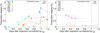 |
Fig. 13. Same as Fig. 12 but with the time after explosion normalized by the length of the photospheric phase, for SNe in Groups 1 and 2 (left panel) and for the other SNe (right panel). The horizontal dashed lines express a zero degree of polarization. The dotted lines are the extrapolation of the first two points that start to show an increase in polarization degree, whose intersection with the dashed line (P = 0) is defined as the timing of the polarization rise (tpol). |
Type, polarization group, and characteristic polarimetric, photometric, and spectroscopic parameters for the 15 SNe in our sample.
3. Photometric and spectroscopic properties
3.1. Photometric properties
Figure 14 shows the light curves of our SN sample, which are corrected for reddening (see Table 1 in Paper I). The SNe have diverse properties in terms of brightness and duration of the photospheric phase. For characterizing the light-curve shapes, we fit the time evolution of the absolute magnitude (M(t)) with the following artificial function, which is composed of two power-law functions and a sigmoid function (see Fig. 15):
![Mathematical equation: $$ \begin{aligned} M(t)&= \frac{-a_{0}}{1+e^{\frac{t-t_{\rm ph}}{{ w}_0}}} + M_{\rm t} \nonumber \\&\quad + \left\{ \begin{array}{ll} s_{\rm p} \left[ t- \left( t_{\rm ph} - { w}_0 \right) \right]&(t \le t_{\rm ph}-{ w}_0) \\ 0&(t_{\rm ph}-{ w}_0 \le t \le t_{\rm ph}+{ w}_0)\\ s_{\rm t} \left[ t- \left( t_{\rm ph} - { w}_0 \right) \right]&(t \ge t_{\rm phm}+{ w}_0), \end{array} \right. \end{aligned} $$](/articles/aa/full_html/2024/01/aa46715-23/aa46715-23-eq1.gif) (1)
(1)
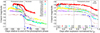 |
Fig. 14. V-band light curves of our sample (left panel) and the same light curves with the time after explosion nomalized by the length of the photospheric phase (right panel). The vertical line and dashed lines indicate the timing of the middle and end of the photospheric phase, respectively. The blue dotted line is the extrapolation of the first point. |
where Mt, a0, tph, w0, sp, and st are free parameters. The best-fit values for these parameters are summarized in Table 2 for each SN.
Best-fit values from the light-curve fitting.
As a characteristic value for the SN brightness, we adopt the V-band absolute magnitude in the middle of the photospheric phase (MV(tph/2)). In order to derive the typical value of the SN bolometric luminosity from the V-band magnitude, we simply assume a 6000 K black-body spectrum. The values of L(tph/2) converted from M(tph/2) are presented in Table 1. In order to derive the Ni mass for each SN, which is also summarized in Table 1, we adopt the empirical method proposed by Hamuy (2003) using the following equations:
![Mathematical equation: $$ \begin{aligned} M_{\rm Ni} = (7.866 \times 10^{-44}) L_{\rm t} \exp \left[ \frac{(t_{\rm ph}+{ w}_{0})/(1+z) -6.1}{111.26} \right] \,{M}_{\odot }, \end{aligned} $$](/articles/aa/full_html/2024/01/aa46715-23/aa46715-23-eq5.gif) (2)
(2)
where Lt is the bolometric luminosity at t = tph + w0, which, in turn, is estimated using the following empirical equation by Hamuy (2001):
 (3)
(3)
where for the bolometric correction (BC), we adopt the value BC = 0.26 ± 0.06 during the tail phase (Hamuy 2001).
In this work, we classify the SNe as Type IIP and IIL based on the values of sp. The SNe with sp < 1 are classified as Type IIP, while the others are classified as Type IIL. Here, the derived value of sp for SN 2006ov indicates it as a Type IIL SN in our criteria (sp > 1; see Sect. 3.1). However, this is just due to the limited photometric data during the photospheric phase (see Sect. 3.1). The photometric and spectroscopic properties of SN 2006ov in Chornock et al. (2010) suggest a class of Type IIP. We therefore classify it as a Type IIP SN in this work. As for the SNe that do not have photometric observations (SNe 2010hv, 2010co, 2001du and 2001dh), we label them as simply Type II in this paper. The photometric classification of the SNe is shown in Table 1.
3.2. Spectroscopic properties
In this paper, we do not discuss the spectroscopic properties of our sample. However, for the purposes of our analysis, we extracted the expansion velocities. In particular, we derived the ejecta velocity at the middle of the photospheric phase derived using the Fe II λ5169 line (v(tph/2)), and used it as a characteristic value. The velocities were estimated from the absorption minima using the spectra presented in Paper I. For SNe 2004dj and 1999em, we adopted the Fe velocity derived by Takáts & Vinkó (2012). The uncertainties on the absorption minima position are evaluated from the spectral dispersion (e.g., ∼3.3 Å pixel−1 for G300V/FORS2/VLT). The derived velocities are shown in Fig. 16 and the values of v(tph/2) are provided in Table 1.
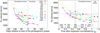 |
Fig. 16. Fe II velocities of our SN sample (left panel) and the velocities with the time after explosion nomalized by the length of the photospheric phase (right panel). The vertical lines are the same as in Fig. 14. The dotted lines are the extrapolation of the first point. |
3.3. SN explosion properties
We estimate the basic SN physical properties (explosion energy:  , ejecta mass:
  , and pre-explosion progenitor radius:
  ) from the SN photometric and spectroscopic properties (typical luminosity:
  , typical duration:
  , typical ejecta velocity:
  , and the 56Ni mass: MNi). Here, we are not interested in deriving precise values for these physical quantities but rather in obtaining some relative scales for the quantities. We therefore use a simple one-zone model of homogeneously expanding gas with radiative diffusion, as proposed by Kasen & Woosley (2009). This is characterized by the following equations:
 (4)
(4)
 (5)
(5)
![Mathematical equation: $$ \begin{aligned}&\widetilde{R}_{\rm p} = \frac{\kappa _{\rm es}}{2 \pi c \sigma _{\rm SB} T_{I}^{4}} \widetilde{t}_{\rm sn}^{-2} \widetilde{L}_{\rm sn}^{2} \widetilde{v}_{\rm sn}^{-4} \left[ 1 - \widetilde{L}_{\rm sn}^{-1} \widetilde{t}_{\rm sn}^{-2} (E_{\rm Ni}t_{\rm Ni} +E_{\rm Co}t_{\rm Co}) \right], \end{aligned} $$](/articles/aa/full_html/2024/01/aa46715-23/aa46715-23-eq15.gif) (6)
(6)
where ENi ≃ 0.6 × 1050(MNi/M⊙) erg and ECo ≃ 1.2 × 1050(MNi/M⊙) erg are the total energy from 56Ni and 56Co decay, with decay times of tNi ≃ 8.8 and tCo ≃ 113 days, respectively. Here, we simply assume that  ,
,  and
and  .
.
We note that, as we assume a constant brightness from radiative diffusion, we cannot apply this analysis to Type IIL SNe in general. However, SN 2013ej is also proposed as a Type IIP SN based on its photometric and spectroscopic properties (e.g., Dhungana et al. 2016). Moreover, its light curve is very similar to those of Type IIP SNe, except for the early bump during the first ∼40 days, which is understood to be the result of a CSM interaction. We therefore conducted this analysis for the Type IIP SNe for which photometric and spectroscopic information is available (SNe 2017gmr, 2012ec, 2012aw, 2008bk, 2007aa, 2006ov, 2004dj and 1999em) as well as for the Type IIL SN 2013ej. The derived values for  ,
,  , and
, and  are summarized in Table 3.
Characteristic SN explosion properties from the SN photometric and spectroscopic properties.
4. Relations between polarimetric, photometric and spectroscopic properties
In this section, we discuss relations between the polarimetric, photometric, and spectroscopic parameters of 11 SNe for which both sets of observations are available (8 Type IIP and 3 Type IIL SNe). Figure 17 shows the relations between the polarimetric (tpol) and photometric parameters (tph, a0, w0, Mt, sp and st). There seems to be no significant correlation between polarization degree and the other photometric parameters. However, the brightness at the tail phase Mt (and thus the 56Ni mass; see below) and the brightness gap between the photospheric and tail phases (a0) might be correlated with tpol in Type IIP SNe, although the limited sample does not allow any firm conclusions to be made.
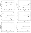 |
Fig. 17. Relations between the polarimetric property (tpol) and photometric properties (tph, a0, w0, Mt, sp and st). The black points represent Type IIP SNe, while gray points do Type IIL SNe. |
Figure 18 shows the relations between the polarimetric parameter (tpol) and the characteristic values from the photometric and spectroscopic observations (M(tph/2), v(tph/2) and MNi). In the Type IIP sample, there may be some correlations: SNe that are brighter and faster and contain a greater amount of 56Ni tend to have more extended aspherical structures. As the Type IIL sample is limited, we cannot conclude anything about their behavior. However, these objects do not seem to follow these correlations. We emphasize that the ejecta velocity estimated from the Fe II absorption minimum is related to the ejecta velocity along the line of sight, and is therefore affected by the viewing angle. Most SNe show peak polarization degrees of ∼1%, implying aspherical structures with a minimum ellipsoidal axial ratio of 1.2:1.0. If the parts of the ejecta forming the Fe II line have such an asphericity, the estimated velocities can have an uncertainty of ± ≳ 10% simply because of the uncertainties on the viewing angle. This effect is more important for SNe that have more aspherical structures in the line-forming regions, that is, in the outer parts of the ejecta above the photosphere. Moreover, the Fe distribution does not necessarily have to be consistent with the overall aspherical structure. In some extreme cases, such as SN 2017gmr, there is a global aspherical structure from the inner core to the outer envelope that might be created by a jet-like explosion and might produce a more aspherical Fe distribution. A larger sample is required to statistically confirm this correlation between the ejecta velocity and the polarimetric parameter taking into account this effect.
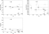 |
Fig. 18. Relations between the polarimetric property (tpol) and the characteristic values from the photometric and spectroscopic observations (M(tph/2), v(tph/2), and MNi). The black points represent Type IIP SNe, while gray points show Type IIL SNe. |
Figure 19 shows the relations between the polarimetric property (tpol) and the SN explosion parameters ( ,
,  ,
,  ). The polarimetric property (tpol) is correlated with the explosion energy (
 ) rather than with the ejecta mass (
 ) and the progenitor radius (
 ): More energetic SNe tend to have more extended aspherical structure in their explosions. We finally note that the absolute values of the SN explosion parameters are not accurate because of limitations to the one-zone model (see Sect. 3.3). Therefore, only a relative comparison between the various SNe is possible. In addition, the largest uncertainties for the SN explosion parameters come from the uncertainty on the viewing angles, which translates to a significant uncertainty on the expansion velocities.
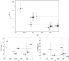 |
Fig. 19. Relations between the polarimetric property (tpol) and the SN explosion parameters ( |


5. Conclusions
In this article, we present an investigation of the continuum polarization of 15 Type II SNe. Our analysis shows that the objects in the sample have diverse properties. Most SNe show low polarization at early phases with a sudden rise to a degree of ∼1% at a certain point during the photospheric phase, followed by a slow decline during the tail phase, with a constant polarization angle. The timing of the polarization rise varies between SNe. We interpret this as the signature of different explosion geometries: some SNe have aspherical structures only in their helium cores, while the asphericity of other SNe reaches out to a significant part of the outer hydrogen envelope, with a common axis through the helium core and the hydrogen envelope. Some SNe show high polarization already at early phases and a change in polarization angle. This indicates multidirectional aspherical structures in their explosions, which might originate from a combination of a common aspherical SN explosion and an aspherical CSM interaction or from a multidirectional SN explosion. An exception in our sample is the Type IIL SN 2017ahn, which has low polarization during both the photospheric and tail phases. As this object is unique in our sample, we cannot conclude as to whether this SN is produced by a completely spherical explosion or is simply the result of a different viewing angle for a similarly aspherical explosion.
The timing of the polarization rise in Type IIP SNe appears to be correlated with their brightness, ejecta velocity, and Ni mass: SNe with higher brightness, higher ejecta velocity, and greater Ni production show more extended asphericities. In particular, there is a clear correlation between the timing of the polarization rise and the explosion energy: the asphericity in the explosions is proportional to the explosion energy (see Sect. 4 and Fig. 19). This implies that the emergence of a global aspherical structure, such as a jet-like structure, might be the key ingredient in the explosion mechanism that produces an energetic SN.
Acknowledgments
We thank Keiichi Maeda, Masaomi Tanaka and Giuliano Pignata for useful discussions. T.N. was supported by a Japan Society for the Promotion of Science (JSPS) Overseas Research Fellowship and was funded by the Academy of Finland project 328898. H.K. was funded by the Academy of Finland projects 324504 and 328898. S.M. was funded by the Academy of Finland project 350458. This research has made use of NASA’s Astrophysics Data System Bibliographic Services.
References
- Anderson, J. P., González-Gaitán, S., Hamuy, M., et al. 2014, ApJ, 786, 67 [Google Scholar]
- Andrews, J. E., Sand, D. J., Valenti, S., et al. 2019, ApJ, 885, 43 [Google Scholar]
- Blondin, J. M., Mezzacappa, A., & DeMarino, C. 2003, ApJ, 584, 971 [NASA ADS] [CrossRef] [Google Scholar]
- Buras, R., Rampp, M., Janka, H. T., & Kifonidis, K. 2006, A&A, 447, 1049 [NASA ADS] [CrossRef] [EDP Sciences] [Google Scholar]
- Chornock, R., Filippenko, A. V., Li, W., & Silverman, J. M. 2010, ApJ, 713, 1363 [Google Scholar]
- Dessart, L., & Hillier, D. J. 2011, MNRAS, 415, 3497 [Google Scholar]
- Dessart, L., Leonard, D. C., John Hillier, D., & Pignata, G. 2021, A&A, 651, A19 [NASA ADS] [CrossRef] [EDP Sciences] [Google Scholar]
- Dhungana, G., Kehoe, R., Vinko, J., et al. 2016, ApJ, 822, 6 [NASA ADS] [CrossRef] [Google Scholar]
- Faran, T., Poznanski, D., Filippenko, A. V., et al. 2014a, MNRAS, 442, 844 [NASA ADS] [CrossRef] [Google Scholar]
- Faran, T., Poznanski, D., Filippenko, A. V., et al. 2014b, MNRAS, 445, 554 [NASA ADS] [CrossRef] [Google Scholar]
- Foglizzo, T. 2002, A&A, 392, 353 [NASA ADS] [CrossRef] [EDP Sciences] [Google Scholar]
- Hamuy, M. A. 2001, PhD Thesis, University of Arizona, USA [Google Scholar]
- Hamuy, M. 2003, ApJ, 582, 905 [NASA ADS] [CrossRef] [Google Scholar]
- Hanke, F., Müller, B., Wongwathanarat, A., Marek, A., & Janka, H.-T. 2013, ApJ, 770, 66 [NASA ADS] [CrossRef] [Google Scholar]
- Herant, M., Benz, W., Hix, W. R., Fryer, C. L., & Colgate, S. A. 1994, ApJ, 435, 339 [NASA ADS] [CrossRef] [Google Scholar]
- Höflich, P. 1991, A&A, 246, 481 [Google Scholar]
- Janka, H.-T. 2012, Ann. Rev. Nucl. Part. Sci., 62, 407 [Google Scholar]
- Janka, H. T., Langanke, K., Marek, A., Martínez-Pinedo, G., & Müller, B. 2007, Phys. Rep., 442, 38 [NASA ADS] [CrossRef] [Google Scholar]
- Kasen, D., & Woosley, S. E. 2009, ApJ, 703, 2205 [NASA ADS] [CrossRef] [Google Scholar]
- Kawabata, K. S., Jeffery, D. J., Iye, M., et al. 2002, ApJ, 580, L39 [NASA ADS] [CrossRef] [Google Scholar]
- Kumar, B., Pandey, S. B., Eswaraiah, C., & Kawabata, K. S. 2016, MNRAS, 456, 3157 [NASA ADS] [CrossRef] [Google Scholar]
- Leonard, D. C., Filippenko, A. V., Ardila, D. R., & Brotherton, M. S. 2001, ApJ, 553, 861 [NASA ADS] [CrossRef] [Google Scholar]
- Leonard, D. C., Filippenko, A. V., Ganeshalingam, M., et al. 2006, Nature, 440, 505 [NASA ADS] [CrossRef] [Google Scholar]
- Li, W., Leaman, J., Chornock, R., et al. 2011, MNRAS, 412, 1441 [NASA ADS] [CrossRef] [Google Scholar]
- Marek, A., & Janka, H. T. 2009, ApJ, 694, 664 [NASA ADS] [CrossRef] [Google Scholar]
- Maund, J. R., Wheeler, J. C., Baade, D., et al. 2009, ApJ, 705, 1139 [NASA ADS] [CrossRef] [Google Scholar]
- Melson, T., Janka, H.-T., & Marek, A. 2015, ApJ, 801, L24 [NASA ADS] [CrossRef] [Google Scholar]
- Nagao, T., Maeda, K., & Tanaka, M. 2018, ApJ, 861, 1 [NASA ADS] [CrossRef] [Google Scholar]
- Nagao, T., Cikota, A., Patat, F., et al. 2019, MNRAS, 489, L69 [CrossRef] [Google Scholar]
- Nagao, T., Patat, F., Taubenberger, S., et al. 2021, MNRAS, 505, 3664 [NASA ADS] [CrossRef] [Google Scholar]
- Nagao, T., Mattila, S., Kotak, R., et al. 2023, A&A, 678, A43 [NASA ADS] [CrossRef] [EDP Sciences] [Google Scholar]
- Patat, F., & Romaniello, M. 2006, PASP, 118, 146 [Google Scholar]
- Patat, F., Cappellaro, E., Danziger, J., et al. 2001, ApJ, 555, 900 [Google Scholar]
- Reilly, E., Maund, J. R., Baade, D., et al. 2016, MNRAS, 457, 288 [NASA ADS] [CrossRef] [Google Scholar]
- Sanders, N. E., Soderberg, A. M., Gezari, S., et al. 2015, ApJ, 799, 208 [NASA ADS] [CrossRef] [Google Scholar]
- Takáts, K., & Vinkó, J. 2012, MNRAS, 419, 2783 [CrossRef] [Google Scholar]
- Takiwaki, T., Kotake, K., & Suwa, Y. 2012, ApJ, 749, 98 [NASA ADS] [CrossRef] [Google Scholar]
- Tanaka, M., Kawabata, K. S., Maeda, K., et al. 2009, ApJ, 699, 1119 [NASA ADS] [CrossRef] [Google Scholar]
- Tartaglia, L., Sand, D. J., Groh, J. H., et al. 2021, ApJ, 907, 52 [NASA ADS] [CrossRef] [Google Scholar]
- Utrobin, V. P., Chugai, N. N., Andrews, J. E., et al. 2021, MNRAS, 505, 116 [NASA ADS] [CrossRef] [Google Scholar]
- Valenti, S., Howell, D. A., Stritzinger, M. D., et al. 2016, MNRAS, 459, 3939 [NASA ADS] [CrossRef] [Google Scholar]
- Wang, L., & Wheeler, J. C. 2008, ARA&A, 46, 433 [Google Scholar]
- Wang, L., Wheeler, J. C., & Höflich, P. 1997, ApJ, 476, L27 [NASA ADS] [CrossRef] [Google Scholar]
- Wongwathanarat, A., Müller, E., & Janka, H. T. 2015, A&A, 577, A48 [NASA ADS] [CrossRef] [EDP Sciences] [Google Scholar]
Appendix A: Polarization degrees and angles of the continuum polarization for the VLT sample
SN 2017gmr
SN 2017ahn
SN 2013ej
SN 2012ec
SN 2012dh
SN 2012aw
SN 2010hv
SN 2010co
SN 2008bk
SN 2001du
SN 2001dh
Appendix B: Spectropolarimetric data for the FORS/VLT sample
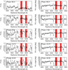 |
Fig. B.1. Spectropolarimetry of SN 2017gmr after ISP subtraction. The red hatching shows the adopted wavelength range for the continuum polarization estimate. |
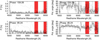 |
Fig. B.10. Same as Figure B.1, but for SN 2001du. |
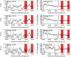 |
Fig. B.11. Same as Figure B.1, but for SN 2001dh. |
All Tables
Type, polarization group, and characteristic polarimetric, photometric, and spectroscopic parameters for the 15 SNe in our sample.
Characteristic SN explosion properties from the SN photometric and spectroscopic properties.
All Figures
|
Fig. 1. Polarization degree and angle of the continuum polarization in SN 2017gmr. |
| In the text | |
|
Fig. 2. Polarization degree and angle of the continuum polarization in SN 2017ahn. |
| In the text | |
|
Fig. 3. Polarization degree and angle of the continuum polarization in SN 2013ej. The explosion component is shown in red. |
| In the text | |
|
Fig. 4. Polarization degree and angle of the continuum polarization in SN 2012ec. |
| In the text | |
|
Fig. 5. Polarization degree and angle of the continuum polarization in SN 2012dh. |
| In the text | |
|
Fig. 6. Polarization degree and angle of the continuum polarization in SN 2012aw. The aspherical explosion component is shown in red. |
| In the text | |
|
Fig. 7. Polarization degree and angle of the continuum polarization in SN 2010hv. |
| In the text | |
|
Fig. 8. Polarization degree and angle of the continuum polarization in SN 2010co. |
| In the text | |
|
Fig. 9. Polarization degree and angle of the continuum polarization in SN 2008bk. |
| In the text | |
|
Fig. 10. Polarization degree and angle of the continuum polarization in SN 2001du. |
| In the text | |
|
Fig. 11. Polarization degree and angle of the continuum polarization in SN 2001dh. |
| In the text | |
|
Fig. 12. Time evolution of the continuum polarization of our SN sample. Here, for SNe 2013ej and 2012aw, we plot the explosion components after the subtraction of the interaction components. |
| In the text | |
|
Fig. 13. Same as Fig. 12 but with the time after explosion normalized by the length of the photospheric phase, for SNe in Groups 1 and 2 (left panel) and for the other SNe (right panel). The horizontal dashed lines express a zero degree of polarization. The dotted lines are the extrapolation of the first two points that start to show an increase in polarization degree, whose intersection with the dashed line (P = 0) is defined as the timing of the polarization rise (tpol). |
| In the text | |
|
Fig. 14. V-band light curves of our sample (left panel) and the same light curves with the time after explosion nomalized by the length of the photospheric phase (right panel). The vertical line and dashed lines indicate the timing of the middle and end of the photospheric phase, respectively. The blue dotted line is the extrapolation of the first point. |
| In the text | |
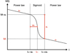 |
Fig. 15. Schematics of the function used for the light-curve fitting (see Eq. (1)). |
| In the text | |
|
Fig. 16. Fe II velocities of our SN sample (left panel) and the velocities with the time after explosion nomalized by the length of the photospheric phase (right panel). The vertical lines are the same as in Fig. 14. The dotted lines are the extrapolation of the first point. |
| In the text | |
|
Fig. 17. Relations between the polarimetric property (tpol) and photometric properties (tph, a0, w0, Mt, sp and st). The black points represent Type IIP SNe, while gray points do Type IIL SNe. |
| In the text | |
|
Fig. 18. Relations between the polarimetric property (tpol) and the characteristic values from the photometric and spectroscopic observations (M(tph/2), v(tph/2), and MNi). The black points represent Type IIP SNe, while gray points show Type IIL SNe. |
| In the text | |
|
Fig. 19. Relations between the polarimetric property (tpol) and the SN explosion parameters ( |
| In the text | |
|
Fig. B.1. Spectropolarimetry of SN 2017gmr after ISP subtraction. The red hatching shows the adopted wavelength range for the continuum polarization estimate. |
| In the text | |
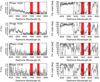 |
Fig. B.2. Same as Figure B.1, but for SN 2017ahn. |
| In the text | |
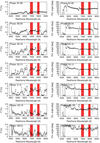 |
Fig. B.3. Same as Figure B.1, but for SN 2013ej. |
| In the text | |
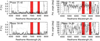 |
Fig. B.4. Same as Figure B.1, but for SN 2012ec. |
| In the text | |
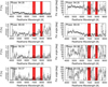 |
Fig. B.5. Same as Figure B.1, but for SN 2012dh. |
| In the text | |
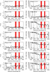 |
Fig. B.6. Same as Figure B.1, but for SN 2012aw. |
| In the text | |
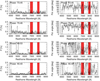 |
Fig. B.7. Same as Figure B.1, but for SN 2010hv. |
| In the text | |
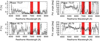 |
Fig. B.8. Same as Figure B.1, but for SN 2010co. |
| In the text | |
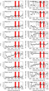 |
Fig. B.9. Same as Figure B.1, but for SN 2008bk. |
| In the text | |
|
Fig. B.10. Same as Figure B.1, but for SN 2001du. |
| In the text | |
|
Fig. B.11. Same as Figure B.1, but for SN 2001dh. |
| In the text | |
Current usage metrics show cumulative count of Article Views (full-text article views including HTML views, PDF and ePub downloads, according to the available data) and Abstracts Views on Vision4Press platform.
Data correspond to usage on the plateform after 2015. The current usage metrics is available 48-96 hours after online publication and is updated daily on week days.
Initial download of the metrics may take a while.