| Issue |
A&A
Volume 678, October 2023
|
|
|---|---|---|
| Article Number | A43 | |
| Number of page(s) | 34 | |
| Section | Stellar structure and evolution | |
| DOI | https://doi.org/10.1051/0004-6361/202346713 | |
| Published online | 29 September 2023 | |
Spectropolarimetry of Type II supernovae
I. Sample, observational data, and interstellar polarization
1
Department of Physics and Astronomy, University of Turku, Vesilinnantie 5, 20014 Turku, Finland
e-mail: This email address is being protected from spambots. You need JavaScript enabled to view it.
2
Aalto University Metsähovi Radio Observatory, Metsähovintie 114, 02540 Kylmälä, Finland
3
Aalto University Department of Electronics and Nanoengineering, PO Box 15500 00076 Aalto, Finland
4
School of Sciences, European University Cyprus, Diogenes street, Engomi, 1516 Nicosia, Cyprus
5
Finnish Centre for Astronomy with ESO (FINCA), University of Turku, Vesilinnantie 5, 20014 Turku, Finland
Received:
20
April
2023
Accepted:
19
July
2023
Abstract
We investigate the polarization spectra of hydrogen-rich core-collapse supernovae (Type II SNe). The polarization signal from SNe contains two independent components: intrinsic SN polarization and interstellar polarization (ISP). From these components, we can study the SN explosion geometry and the dust properties in their host galaxies or in the Milky Way. In this first paper, we employ a newly improved method to investigate the properties of the ISP components of 11 well-observed Type II SNe. Our analyses revealed that 10 of these 11 SNe showed a steady ISP component with a polarization degree of ≲1.0%, while one SN was consistent with zero ISP. As for the wavelength dependence, SN 2001dh (and possibly SN 2012aw) showed a non-Milky-Way-like ISP likely originating from the interstellar dust in their respective host galaxies: their polarization maxima were located at short wavelengths (≲4000 Å). Similar results have been obtained previously for highly reddened SNe. The majority of the SNe in our sample had uncertainties in the wavelength dependence of their ISP components that were too large for further consideration. Our work demonstrates that further investigation of the ISP component of the SN polarization, by applying this method to a larger SN sample, can provide new opportunities to study interstellar dust properties in external galaxies.
Key words: supernovae: general / techniques: polarimetric / dust / extinction
© The Authors 2023
 Open Access article, published by EDP Sciences, under the terms of the Creative Commons Attribution License (https://creativecommons.org/licenses/by/4.0), which permits unrestricted use, distribution, and reproduction in any medium, provided the original work is properly cited.
This article is published in open access under the Subscribe to Open model. This email address is being protected from spambots. You need JavaScript enabled to view it. to support open access publication.
1. Introduction
The polarization signal from supernovae (SNe) contains information on the explosion geometry, which is directly related to the explosion mechanism. Past studies using polarimetry have revealed that core-collapse SNe are generally aspherical explosions (e.g., Wang & Wheeler 2008, for a review). At the same time, the SN polarization usually also carries an extrinsic component, that is, the interstellar polarization (ISP), which originates from the differential extinction of the SN light by aspherical interstellar (IS) dust grains aligned with the IS magnetic field. It is important to properly remove this ISP component from polarimetric observations of SNe in order to estimate the intrinsic SN polarization, which enables us to study their explosion geometries.
There have been several attempts to estimate the ISP components from the spectropolarimetry of SNe (e.g., Trammell et al. 1993; Tran et al. 1997; Wang et al. 1997, 2001; Leonard et al. 2000, 2001, 2002a, 2005; Howell et al. 2001; Chornock et al. 2006; Patat et al. 2012; Mauerhan et al. 2015; Inserra et al. 2016; Reilly et al. 2017; Stevance et al. 2017, 2019; Nagao et al. 2019, 2021). These methods rely mainly on one of the following assumptions: (1) the emission peaks of the P-Cygni lines have no intrinsic polarization due to multiple resonant scatterings and/or re-combinations of the photons; (2) the polarization signal from SNe at a sufficiently late phase, when the electron density in the ejecta becomes small enough, is purely from the ISP; or (3) a high level of polarization that remains constant in time (≳1%) is mainly from the ISP.
Precise estimation of the ISP component in SN polarization is important not only for deriving the SN intrinsic polarization, but also for investigating the properties of the IS dust. In fact, as SNe are intrinsically bright, using the ISP component in the SN polarization signal leads to probing the dust properties in distant galaxies beyond the Milky Way (MW). It is known that the peak wavelength of the ISP (λmax) is related to the total-to-selective extinction ratio (RV), as RV ∼ 5.5λmax [μm] (Serkowski et al. 1975), which is a key parameter of extinction. From the polarization maxima of several reddened SNe at wavelengths shorter (λmax ≲ 0.4 μm; e.g., Patat et al. 2015; Zelaya et al. 2017; Chu et al. 2022; Nagao et al. 2022) than the typical MW ISP (λmax ∼ 0.545 μm; Serkowski et al. 1975), the presence of dust grains that are peculiarly small in comparison to the MW dust has been inferred. At the same time, some reddened Type II SNe (SN 1999gi and SN 2022ame; Leonard et al. 2001; Nagao et al. 2022) show MW-like polarization curves for their host-galaxy ISP (λmax ∼ 0.53 μm), implying the existence of MW-like dust in their host galaxies. These facts indicate that there is a diversity in the properties of the IS dust in different galaxies and/or in different locations in galaxies (Nagao et al. 2022).
As SNe typically do have some intrinsic polarization (≲1%; e.g., Wang & Wheeler 2008), investigations of the properties of IS dust in external galaxies using SN polarization have previously been mainly applied to highly reddened SNe, whose ISP dominates the polarization signal. The application of this method to real observations has been very limited, due principally to the following reasons: (1) SNe with high extinction are intrinsically rare; (2) such highly reddened objects are optically faint, and therefore rejected for follow-up; or (3) spectropolarimetry of faint objects requires access to large telescopes.
In this paper (Paper I), we describe and implement an improved method compared to those presented in Nagao et al. (2019, 2021) to estimate the ISP component from spectropolarimetric observations of 11 H-rich core-collapse SNe (hereafter Type II, including Type IIP and IIL)1, that is, SNe whose ISP is embedded in their intrinsic SN polarization.
This paper is organized as follows. In Sect. 2, we present our SN sample. In Sect. 3, we present our observational data and describe our data reduction procedures. Then, we explain our method for estimating the ISP and determine and discuss the properties of the ISP in Sect. 4. We summarise our findings in Sect. 5. In a follow-up paper (Nagao et al. 2023, hereafter Paper II), we discuss the properties of the intrinsic SN polarization of 15 SNe from our SN sample, including their photometric and spectroscopic properties, and the relations between these properties.
2. SN spectropolarimetric sample
We collected from the literature and archives all the publicly available spectropolarimetric data of Type II SNe that have multi-epoch observations. Our sample consists of 11 Type II SNe observed with the FOcal Reducer/low-dispersion Spectrograph (FORS1 and FORS2, hereafter FORS; Appenzeller et al. 1998) mounted on the Very Large Telescope (VLT) at the European Southern Observatory (ESO), in addition to 4 Type II SNe observed with other instruments. The details of the SNe in our sample are summarized in Table 1 and also in the following subsections.
Details of the SNe.
2.1. SN 2017gmr
SN 2017gmr was discovered by the ‘Distance Less Than 40 Mpc’ SN search (DLT40; Tartaglia et al. 2018) on 4.27 September 2017 UT (58 000.27 MJD; Valenti et al. 2017), in the host galaxy NGC 0988. The redshift of the host galaxy is z = 0.005037 ± 0.000017, which is taken from the ‘HI Parkes All Sky Survey’ (HIPASS) catalog Koribalski et al. (2004) via the NASA/IPAC Extragalactic Database (NED)2. It was classified as a core-collapse SN within a few days of the discovery (Pursimo et al. 2017). The last non-detection of the object was on 2.23 September 2017 UT (57 998.23 MJD), approximately two days before the discovery (Valenti et al. 2017). We adopted 57 999.09 MJD as the explosion date of SN 2017gmr, with a distance modulus of μ = 31.46 ± 0.15 mag, and a total line-of-sight extinction of AV = 1.14 mag (Andrews et al. 2019).
2.2. SN 2017ahn
SN 2017ahn was discovered on 8.29 February 2017 UT (57 792.29 MJD; Tartaglia et al. 2017), by DLT40. It is located in NGC 3318 at z = 0.009255 ± 0.000021 (from the HIPASS catalog via NED), and was classified as a Type II SN within a day of the discovery (Hosseinzadeh et al. 2017). The last non-detection was on 7.23 February 2017 UT (57 791.23 MJD), approximately one day before the discovery (Tartaglia et al. 2017). We adopted 57 791.76 MJD as the explosion date of SN 2017ahn (Tartaglia et al. 2021), μ = 32.59 ± 0.43 mag (Sorce et al. 2014), and AV = 0.82 mag (Tartaglia et al. 2021).
2.3. SN 2013ej
SN 2013ej was discovered by the Lick Observatory Supernova Search on 25.45 July 2013 UT (56 498.45 MJD; Kim et al. 2013). It is located in Messier 74 at z = 0.002192 ± 0.000003 (Lu et al. 1993). The last non-detection of the object was on 23.54 July 2013 UT (56 496.54 MJD), approximately two days before the discovery (Shappee et al. 2013). We adopted 56 496.9 MJD as the explosion date of SN 2013ej (Dhungana et al. 2016), μ = 29.91 ± 0.16 mag (Huang et al. 2015), and AV = 0.19 mag (Dhungana et al. 2016).
2.4. SN 2012ec
SN 2012ec was discovered on 11.04 August 2012 UT (56 150.04 MJD; Monard et al. 2012). It is located in NGC 1084 at z = 0.004693 ± 0.000013 (from the HIPASS catalog via NED). The object was classified as a Type II SN on 17.7 August 2012 UT (Takaki et al. 2012). The last non-detection of the object was on 28.75 March 2012 UT (56 014.75 MJD; Monard et al. 2012). We adopted 56 143.00 MJD as the explosion date of SN 2012ec (Barbarino et al. 2015), μ = 31.10 ± 0.06 mag (Springob et al. 2009), and AV = 0.45 mag (Barbarino et al. 2015).
2.5. SN 2012dh
SN 2012dh was discovered on 26.98 June 2012 UT (56 104.98 MJD; Maza et al. 2012). It is located in ESO 443-G80 at z = 0.007055 ± 0.000007 (from the HIPASS catalog via NED). The object was classified as a Type II SN by the spectra obtained on 28.84 June, 30.84 June, and 2.84 July 2012 UT (Maza et al. 2012). The last non-detection of the object was on 23.11 June 2012 UT (56 101.11 MJD; Maza et al. 2012). Based on the spectrum obtained on 7 July 2012 UT with the Nordic Optical Telescope, Fraser et al. (2012) suggested that this SN was discovered soon after explosion. We adopted the discovery date of 56 104.98 MJD as the explosion date of SN 2012dh and μ = 31.85 ± 0.45 mag (Tully et al. 2016). Due to the lack of significant IS Na I D absorption lines originated from the host galaxy in our spectra, we ignored the extinction in the host galaxy. We only took the extinction value of AV = 0.20 mag from the MW extinction into account (Schlafly & Finkbeiner 2011).
2.6. SN 2012aw
SN 2012aw was discovered on 16.86 March 2012 UT (56 002.86 MJD; Fagotti et al. 2012). It is located in M 95 at z = 0.002595 ± 0.000013 (from the HIPASS catalog via NED). The object was classified as a Type II SN on 19.5 March 2012 UT (Itoh et al. 2012). The last non-detection of the object was on 15.27 March 2012 UT (56 001.27 MJD; Poznanski et al. 2012). We adopted 56 002.10 MJD as the explosion date of SN 2012aw (Barbarino et al. 2015), μ = 30.01 ± 0.09 mag (de Jaeger et al. 2019), and AV = 0.23 mag (Bose et al. 2013).
2.7. SN 2010hv
SN 2010hv was discovered on 18.18 August 2010 UT (55 426.18 MJD; Pignata et al. 2010). It is located in 2MASX J23242536-1902139 at z = 0.024280 ± 0.000043 (from the HIPASS catalog via NED). The last non-detection of the object was on 2.15 August 2010 UT (55 410.15 MJD; Pignata et al. 2010). We adopted 55 418.2 ± 8.0 MJD, which is halfway between the discovery and the last non-detection dates, as the explosion date of SN 2010hv, and considered the time from the last non-detection to the discovery as its uncertainty.
2.8. SN 2010co
SN 2010co was discovered on 6.105 May 2010 UT (55 322.105 MJD; Monard 2010). It is located in NGC 6862 at z = 0.014026 ± 0.000017 (from the HIPASS catalog via NED). The object was classified as a Type II SN on 20 May 2010 UT (Morrell 2010; Green 2010). The last non-detection of the object was on 13.144 April 2010 UT (55 299.144 MJD; Monard 2010). We adopted 55 310.6 ± 11.5 MJD, which is halfway between the discovery and the last non-detection dates, as the explosion date of SN 2010co, and considered the time from the last non-detection to the discovery as its uncertainty.
2.9. SN 2008bk
SN 2008bk was discovered on 25.141 March 2008 UT (54 550.141 MJD; Monard 2008). It is located in NGC 7793 at z = 0.000767 ± 0.000013 (from the HIPASS catalog via NED). The object was classified as a Type II SN on 12.4 April 2008 UT (Morrell & Stritzinger 2008). The last non-detection of the object was on 2.742 January 2008 UT (54 467.742 MJD; Monard 2008). We adopted 54 549.50 MJD as the explosion date of SN 2008bk (Van Dyk et al. 2012b), μ = 27.66 ± 0.04 mag (Zgirski et al. 2017), and AV = 0.07 mag (Van Dyk et al. 2012b).
2.10. SN 2007aa
SN 2007aa was discovered on 18.308 February 2007 UT (54 149.308 MJD; Doi et al. 2007). It is located in NGC 4030 at z = 0.004887 ± 0.000013 (from the HIPASS catalog via NED). The object was classified as a Type II SN on 19.24 February 2007 UT (Folatelli et al. 2007). The last non-detection of the object was on 12.36 March 2005 UT (Doi et al. 2007). We adopted 54 126.7 MJD as the explosion date of SN 2007aa, which was estimated in Gutiérrez et al. (2017). We adopted the distance modulus of μ = 32.38 ± 0.20 mag toward SN 2007aa, as estimated in Tully et al. (2013). Due to the lack of significant IS Na I D absorption lines originated from the host galaxy in our spectra and the minimal ISP Chornock et al. (2010), we ignored the extinction in the host galaxy. We took only the extinction from the MW, AV = 0.07 mag, into account Schlafly & Finkbeiner (2011).
2.11. SN 2006ov
SN 2006ov was discovered on 24.86 November 2006 UT (54 063.86 MJD; Nakano et al. 2006). It is located in NGC 4303 at z = 0.005224 ± 0.000007 (from the HIPASS catalog via NED). The object was classified as a Type II SN on 25.56 November 2006 UT (Blondin et al. 2006). The last non-detection of the object was on 4 May 2006 UT (Nakano et al. 2006). We adopted 53 974 MJD as the explosion date of SN 2006ov (Li et al. 2007) and μ = 30.5 ± 0.4 mag (Spiro et al. 2014). Due to the lack of significant IS Na I absorption lines originated from the host galaxy in our spectra and the minimal ISP (Chornock et al. 2010), we ignored the extinction in the host galaxy. We took only the MW extinction, AV = 0.06 mag, into account (Schlafly & Finkbeiner 2011).
2.12. SN 2004dj
SN 2004dj was discovered on 31.76 July 2004 UT (53 217.76 MJD; Nakano et al. 2004). It is located in NGC 2403 at z = 0.000445 ± 0.000001 (from the HIPASS catalog via NED). The object was classified as a Type II SN on 3.17 August 2004 UT (Patat et al. 2004). The last non-detection of the object was on 11 October 2002 UT (Nakano et al. 2004). We adopted 53 186.5 MJD as the explosion date of SN 2004dj (Chugai et al. 2005), μ = 27.70 ± 0.19 mag, and AV = 0.22 mag (Vinkó et al. 2006).
2.13. SN 2001du
SN 2001du was discovered on 24.7 August 2001 UT (52 145.7 MJD; Evans et al. 2001). It is located in NGC 1365 at z = 0.005457 ± 0.000003 (from the HIPASS catalog via NED). The object was classified as a Type II SN on 2.05 September 2001 UT (Smartt et al. 2001). The last non-detection of the object was on 23.7 August 2001 UT (52 144.7 MJD; Evans et al. 2001). We adopted 52 145.2 ± 0.5 MJD, which is halfway between the discovery and the last non-detection dates, as the explosion date of SN 2001du and considered the term from the last non-detection to the discovery as its uncertainty.
2.14. SN 2001dh
SN 2001dh was discovered on 22.88 July 2001 UT (52 112.88 MJD; Chassagne 2001). It is located in ESO 340-G9 at z = 0.008700 ± 0.000017 (from the HIPASS catalog via NED). The object was classified as a Type II SN on 8 August 2001 UT (Patat et al. 2001). The last non-detection of the object was on 26.1 June 2001 UT (52 086.1 MJD; Chassagne 2001). We adopted 52 099.5 ± 13.4 MJD, which is halfway between the discovery and the last non-detection dates, as the explosion date of SN 2001dh, and considered the term from the last non-detection to the discovery as its uncertainty.
2.15. SN 1999em
SN 1999em was discovered on 29.44 October 1999 UT (51 480.44 MJD; Li 1999). It is located in ESO 340-G9 at z = 0.008700 ± 0.000017 (from the HIPASS catalog via NED). The object was classified as a Type II SN on 29.7 October 1999 UT (Deng et al. 1999). The last non-detection of the object was on 20.45 October 1999 UT (51 471.45 MJD; Li 1999). We adopted 51 475.1 MJD as the explosion date of SN 1999em (Leonard et al. 2002b), μ = 30.34 ± 0.24 mag (Leonard et al. 2003), and AV = 0.31 mag (Leonard et al. 2002b).
3. Observational data and data reduction
3.1. Spectropolarimetric data
We collected spectropolarimetric data of the VLT sample through the ESO Science Archive Facility3, reanalyzed the data, and derived the values for the ISP and the intrinsic SN polarization. The details of the spectropolarimetric observations of the VLT sample are shown in Table 2. The observation logs are provided in Appendix A. To increase the signal-to-noise ratio, we combined the specstropolarimetric data obtained at similar epochs, checking the consistency of the polarization signal. We note that the data qualities of the observations at the last (third) epoch for SN 2010co are too poor to obtain the polarization signal, where the polarization due to the photon shot noise and the variations within different observation frames in this epoch are larger than the polarization signal. Therefore, we have not used the last epoch of the data for SN 2010co in our analysis. For the SNe observed with other instruments, we have instead adopted the derived values for the ISP and the intrinsic SN polarization from the literature: Leonard et al. (2001) for SN 1999em, Leonard et al. (2006) for SN 2004dj, and Chornock et al. (2010) for SN 2006ov and SN 2007aa.
Details of the SNe in the VLT sample.
For the VLT sample, the details of the instrumentation and the data reduction procedure are the same as outlined in Nagao et al. (2019). All of the observations used the optimal set of half-wave retarder-plate (HWP) angles, namely, 0, 45.0, 22.5, and 67.5 degrees (e.g., Patat & Romaniello 2006) and employed the low-resolution G300V grism. The observations were taken with different charge-coupled devices (CCDs), and some observations used an order-sorting filter, whereas others did not (see Table 2). The raw data were reduced using standard methods described in Patat & Romaniello (2006) and the Image Reduction and Analysis Facility (IRAF; Tody 1986, 1993). The ordinary and extraordinary beams of the spectropolarimetric data were extracted with a fixed aperture size of 10 pixels. The extracted spectra were resampled to 5 Å bins in Paper I and 50 Å bins in Paper II for better signal-to-noise ratios. The HWP zeropoint angle chromatism was corrected based on the tabular data in the FORS2 user manual4. The wavelength scale was corrected to the rest frame based on the host-galaxy redshifts (see Table 1). The polarization bias in the polarimetric spectra was removed according to the standard procedure developed by Wang et al. (1997).
3.2. Photometric data
We also collated publicly available V-band light curves for ten SNe in our sample from the literature (see Table 3). Here, the data of SN 2012ec, SN 2012aw, SN 2008bk, and SN 1999em were obtained through the Open Supernova Catalog (Guillochon et al. 2017). For SN 2007aa, we used previously unpublished data from the Calar Alto Observatory (Appendix B). We used Vega-based magnitudes throughout.
References of the light-curve data.
3.3. Spectroscopic data
We used the spectra obtained as the spectropolarimetric observations for the VLT sample (see Table 2). These spectra are provided in Appendix C. The spectra of SN 2006ov are taken from Spiro et al. (2014) through the Supernova Open Catalog. In addition, we used our unpublished new spectroscopic data for SN 2007aa (see Appendix B for details). For SN 2004dj and SN 1999em, we adopted the derived values for the Fe II velocity in Takáts & Vinkó (2012) instead of analyzing the spectra by ourselves (see Paper II).
4. Interstellar polarization
In this section, we describe our method for determining the ISP component of the SN polarization and apply this method to the spectropolarimetric data of the VLT sample (see Table 2).
4.1. ISP estimation
The continuum regions in the spectra of most Type II SNe are intrinsically polarized due to scattering in an aspherical photosphere. This polarization is time dependent and typically most prominent at the beginning of the tail phase (≲1.0%; e.g., Wang & Wheeler 2008; Nagao et al. 2019). This fact must be taken into account for the determination of the ISP in Type II SNe. For the extraction of the ISP signal from the polarimetric spectra, we adopted a similar strategy as described in Nagao et al. (2019, 2021), which assumes that emission peaks of strong spectral lines carry no intrinsic polarization signal, due to the depolarization of the underlying continuum by the unpolarized line emission. In reality, the prominent emission lines (e.g., Hαλ6563 and the Ca II triplet λ8498/8542/8662) do display a nonvanishing polarization with an angle that slightly differs from that measured in other spectral regions (see Fig. 1). Ten of the 11 SNe in our sample show such a nonzero polarization at line peaks (see Appendix D), which we attribute to the ISP. Only in SN 2010hv is the polarization at the emission peaks consistent with zero within the uncertainties (see Fig. D.7). Hence, we assume that its ISP component is zero. All polarization spectra of our sample are shown in Appendix D.
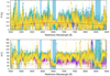 |
Fig. 1. Polarization degree P (top panel) and angle θ (bottom panel) for SN 2017gmr at five different epochs: 58045.60, 58067.24, 58099.86, 58108.76, and 58 134.93 (MJD; purple, green, sky-blue, orange, and yellow symbols, respectively). The data are binned to 5 Å. The gray lines at the bottom of each plot represent the total-flux spectra on 58 134.93 (MJD). The red lines show the polarization degree and angle of the ISP as approximated by P(λ) = Pmaxexp[−Kln2(λmax/λ)] with fixed values of Pmax = 0.35, λmax = 6400 Å and K = 4.0, and θISP = 33.37. The blue shading shows the wavelength windows at the adopted lines, where at all epochs the flux was > 1.1 times higher than in the nearby continuum regions. |
For the ISP measurements, we adopted an improved version of the method from Nagao et al. (2019, 2021). In this paper, we adopted the strong lines due to Hβλ4861, Fe II λ4924, Na I D λ5890/5896, Hαλ6563, and the Ca II triplet λ8498/8542/8662. We evaluated the ISP in windows where the line flux exceeds 1.1 times the continuum level in the flux spectrum normalized by the continuum (see Appendix C). This ensures that the selected signal is dominated by the depolarized line emissions compared to the possibly polarized continuum radiation. We chose such ISP regions individually for each epoch in the 5-Å-binned polarization spectra (blue-shaded regions in Figs. 1, 2, and D.1–D.11). In the following processes, when calculating an average value using the 5-Å binned polarization signals in these ISP regions, we use an average of polarization degrees or angles, taking their errors (but not the flux levels) into account. The efficiency of depolarization by line scattering is different for different lines and also depends on the SN phase at the time of the observation. Therefore, assuming that the ISP is time independent, we averaged, in each wavelength bin (5-Å bin), the polarization degrees from all epochs. In this process, we removed the polarization signals whose polarization degree differed from the average value by more than one standard deviation (1σ), in each 5-Å bin, and repeated this step to revise the epoch-averaged value until all used values satisfied the 1σ criterion. Then, assuming that the polarization angle of the ISP has a constant value in wavelengths, we eliminated epoch-averaged polarization signals with polarization angles differing by more than 1σ from the average for all the epoch-averaged polarization signals. After this elimination, we recalculated the average value of the polarization angle for all the remaining epoch-averaged polarization signals, and repeated this elimination process until all remaining values satisfied the 1σ criterion. Finally, for each line, we also excluded the polarization signals with degrees deviating by more than 1σ from the averaged value in the line-specific wavelength window, until all surviving values satisfied the 1σ criterion.
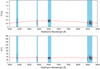 |
Fig. 2. Polarization degree P (top panel) and angle θ (bottom panel) selected for the determination of the ISP in SN 2017gmr. The red lines and the blue-shaded areas are the same as in Fig. 1. In each wavelength bin, the ISP values are the average over all five epochs, after removal of outliers as described in Sect. 4.1. The red lines show the best-fit ISP from Sect. 4.1 and Table 4. |
As an example, Fig. 2 shows the polarization degree and angle of the signals selected as ISP in the polarization spectrum of SN 2017gmr. The average polarization angle of the ISP signals (∼32°) clearly differs from that of the continuum component (∼95°; Nagao et al. 2019, see also Fig. 1). Since the depolarization by line scattering in the relatively weaker lines (Hβ, Fe II, and Na) is inefficient, the number of selected polarization signals is smaller than for the Hα and Ca II lines.
4.2. ISP properties
After the selection of the ISP signals, we calculated the wavelength dependence of the ISP by χ2 fitting of the selected ISP signals with the classical Serkowski function (Serkowski et al. 1975): P(λ) = Pmaxexp[−Kln2(λmax/λ)]. We investigated the parameter ranges of 0.0 ≤ Pmax ≤ 3.0 [%], 100 ≤ λmax ≤ 10 000 [Å], and 0.0 ≤ K ≤ 5.0, with steps of 0.01 [%], 100 [Å], and 0.1, respectively. We calculated the values of the reduced chi-square ( ) for all possible combinations of the fitting parameters, and obtained the best-fit values and the 1σ confidence levels in a 3D grid. The best-fit values and their
  values are shown in Table 4. The values of
  (≲1) are satisfactorily small, as expected if the ISP components are well fitted by the Serkowski et al. (1975) function. However, these good fits can also be due to the small numbers of two to five wavelength windows used.
In Fig. 3, we present the best-fit values with their 1σ confidence levels on the λmax-K plane. For some SNe, the confidence areas are too large to allow us to infer similarities with the ISP properties of MW stars or Type Ia SNe (SN 2017gmr, SN 2017ahn, SN 2012ec, SN 2012dh, SN 2010co, SN 2008bk, and SN 2001du). Nevertheless, some objects (SN 2013ej, SN 2012aw, and SN 2001dh) do show relatively small confidence areas that are closer to the Type Ia SN population than the MW-star population, even though the areas for SN 2013ej and SN 2012aw include small parts of the MW distribution. In addition, the sample displays large spreads in the values of λmax and K. For example, SN 2001dh deviates from all other SNe, and there is only a little overlap between the 1σ confidence areas for SN 2013ej and SN 2017gmr. Such diversity is also seen in the sample of Type Ia SNe (represented by the black crosses in Fig. 3). The different observational errors and wavelength windows used in the ISP determination for our sample affect the accuracy of the derived best-fit values for the fitting parameters (Pmax, λmax, and K) and the fitting errors. However, since the  values are already small for the best fits (see Table 4), the current fitting-error areas in Fig. 3 are the largest for our observational data and method. In the λmax versus K diagram, the error zones will shrink with an increase in the number of usable wavelength windows and with a reduction in the observational uncertainties. Therefore, with the spectropolarimetry of highly extincted SNe whose ISP dominates their polarization, a better determination of the wavelength dependence of the ISP is possible (e.g., Patat et al. 2015; Nagao et al. 2022).
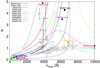 |
Fig. 3. ISP λmax–K diagram for the Type II SNe in this study. Several Type Ia SNe (black crosses; Patat et al. 2015; Zelaya et al. 2017; Cikota et al. 2018) and a large number of MW stars (gray crosses; Whittet et al. 1992) are also included. The colored points show the best-fit values of the Type II SNe, and the lines represent the 1σ confidence intervals for the fitting. |
The wavelength dependence of the polarization for the three Type II SNe with relatively small error ranges (SN 2013ej, SN 2012aw, and SN 2001dh) is presented in Fig. 4. As with the Type Ia SNe also included in this figure, their polarization maxima are at wavelengths of 4000 Å or shorter. This is in stark contrast to the typical Galactic star HD43384, the polarization of which peaks near 5500 Å, although SN 2013ej and SN 2012aw can be consistent with some MW stars within the diversity of MW stars. Some of the fitted λmax values for Type II SNe fall outside the wavelength range (∼4000 to ∼9000 Å) of the observations (see Fig. 3). However, this does not affect the qualitative conclusion of a fundamental difference (mainly in K) between SN 2001dh and the MW stars because the ISP peaks for the MW objects are in this wavelength range (∼4000 to ∼9000 Å).
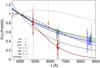 |
Fig. 4. Wavelength dependence of the ISP (normalized to the polarization at 4000 Å) toward SN 2013ej, SN 2012aw, and SN 2001dh (colored points) with their Serkowski law best fits (colored lines). For comparison, the data of three Type Ia SNe (SN 2014J, SN 2008fp, and SN 2006X; Patat et al. 2015) and a Galactic star (HD 43384; Cikota et al. 2018) are also plotted. |
Several of our data sets have been analyzed before (see the references in Table 2). Here, we briefly compare our present results with the past analyses and discuss the differences. The best-fit ISP derived in our previous papers for SN 2017gmr and SN 2017ahn (Nagao et al. 2019, 2021) are consistent within the uncertainties with those presented here (see Fig. 3): Pmax = 0.4%, λmax = 4900 Å, and K = 1.1 for SN 2017gmr (Nagao et al. 2019) and Pmax = 2.05%, λmax = 200 Å, and K = 0.1 for SN 2017ahn (Nagao et al. 2021). The values of λmax and K for SN 2013ej (Pmax = 1.32%, λmax = 3300 Å, and K = 1.0) derived in Nagao et al. (2021) are only marginally consistent with those in this paper, being slightly outside the 1σ error range. This is due to the mildly modified method applied in the present work. Also, in the previous paper, we used all the emission lines, including weaker lines, which might include incompletely depolarized signals, while in this paper we limit the fit to the strong lines (Hβ, Fe II, Na, Hα, and the Ca II triplet). In addition, in our previous work, we determined the polarization angle of the ISP as θ = 110 degrees by eye, but derived a different value of θ = 105 ± 0.6 degrees in this work. These small differences likely give rise to the slightly different best-fit values.
The ISP estimated by Leonard et al. (2021) for SN 2013ej (Pmax = 0.79, λmax = 5100 Å, and K = 1.28) is slightly different from our values. The reason is that Leonard et al. (2021) only used the Hα and Ca II lines and limited the admitted parameter ranges to 0.6 < K < 1.5 and 5000 Å < λmax < 5500 Å, respectively. This leads to a slightly different ISP wavelength dependence from ours, especially at shorter wavelengths. However, the ISP with the largest λmax in the 1σ area (Pmax = 1.01 %, λmax = 4100 Å, and K = 1.2) is reasonably similar, because we used the same data with similar methods. In addition, Leonard et al. (2021) concluded that the ISP of SN 2013ej originated from the MW dust based on the Na I D features and that the polarization peak of the ISP should be located around 5250 Å, based on the wavelengths of peak polarization observed for two Galactic stars close to the line of sight of SN 2013ej. Taking this into account, the correct ISP for SN 2013ej should be relatively close to the above case on the 1-σ border (Pmax = 1.01%, λmax = 4100 Å, and K = 1.2).
Dessart et al. (2021) estimated the ISP wavelength dependence for SN 2012aw under slightly different assumptions from ours. Their derived best-fit values (Pmax = 0.45, λmax = 5535 Å, K = 3.37, and θ = 127°) are outside of the 1σ error region of our best-fit values (see Fig. 3). This difference probably originates mainly from the different estimates of the polarization degree at blue regions, such as those around the Hβ line. We notice that the two methods differ in several aspects: Dessart et al. (2021) assumed a relation between K and λmax derived for the ISP in the MW (K = 1.13 + 0.000405(λmax − 5500); Cikota et al. 2018), while we did not use such a constraint in the fittings of the wavelength dependence of the polarization. On the other hand, we introduced several rejection criteria for incompletely depolarized signals (see Sect. 4.1). Our estimated polarization degree at Hβ is ∼0.8%, while Dessart et al. (2021) found ∼0.4%. This difference may be explained by the fact that we used the line-emission regions only, while Dessart et al. (2021) may have included parts of the absorption components. However, the ISP with the largest λmax in our the 1σ area (Pmax = 0.66%, λmax = 5200 Å, and K = 1.5) is reasonably close to their value, because we used the same data with similar methods.
4.3. ISP due to MW dust versus dust in the host galaxies
ISP can originate not only from dust in the host galaxies, but also from MW dust. The extinction values adopted for the MW reddening of the SNe in our sample are presented in Table 5. From these values and the empirical relation between the extinction and the polarization (P ≤ 9E(B − V); Serkowski et al. 1975), we can estimate the maximum expected polarization degree due to MW dust (Pmax, MW; see Table 5). Here, this maximum polarization is attained in the extreme case when all of the MW-dust grains along the line of sight are aligned in the same direction. Therefore, we expect the MW ISP to fall into the inequality domain of the relation of Serkowski et al. (1975).
Extinction within the MW towards the sample SNe.
Since for some SNe in our sample (SN 2017ahn, SN 2012ec, SN 2012dh, SN 2010hv, and SN 2001du; see Table 5) the polarization degree at 6000 Å (P(6000); see Table 5) is less than (and in some cases comparable to) the maximum values of the Serkowski et al. (1975) relation, their ISP may be partly, or even completely, due to MW dust. This might be the reason why the ISP components of these Type II SNe are consistent not only with those of Type Ia SNe, but also with those of MW stars. However, the other Type II SNe (SN 2017gmr, SN 2013ej, SN 2012aw, SN 2010co, SN 2008bk, and SN 2001dh) show an ISP in excess of the Serkowski et al. (1975) maximum, which may indicate that the contribution by host-galaxy dust is significant or even dominates. In fact, in the cases of SN 2017gmr and SN 2012aw, the extinction in the host galaxies is estimated to be larger than the MW extinction (see Andrews et al. 2019; Van Dyk et al. 2012a), and the maximum polarization from the host extinction based on the Serkowski et al. (1975) relation is larger than the observed ISP. On the contrary, since no significant IS Na I D absorption lines originated from the host galaxy were seen in the high-resolution spectra of SN 2013ej and SN 2008bk (Van Dyk et al. 2012b; Bose et al. 2015), the above estimation of the large host contribution to the ISP should be wrong for these SNe. It is more reasonable to consider the origin of the ISP of these SNe as the MW dust, and they are extreme cases in the Serkowski et al. (1975) relation, where the polarization degrees are slightly higher than the maximum polarization based on the Serkowski et al. (1975) relation. As for SN 2010co and SN 2001dh, there is no available high-resolution spectrum, meaning we cannot quantitatively discuss the extinction in their host galaxies or check the validity of the above interpretation as the large host contribution to the ISP. The MW dust may contribute to the ISP as significantly as does the host-galaxy dust. The MW contribution to the total net polarization degree would be maximal if all the dust grains along the line of sight were aligned in the same direction in both the MW and the host galaxy. Since this is unlikely to be generally the case, we conclude that the ISP of SN 2010co and SN 2001dh likely originates from the dust in their host galaxies.
The ISP angle traces the direction of the magnetic field in the region where the ISP is formed, since this occurs through the differential absorption of the electromagnetic wave by aspherical dust grains aligned with the local magnetic field (e.g., Davis & Greenstein 1951). The direction of the magnetic field in a spiral galaxy globally follows the direction of the spiral arms (e.g., Beck 2015), even though the magnetic field and thus the ISP might suffer local perturbations, e.g., from SNe (Ntormousi 2018). Type II SNe generally occur in late-type galaxies, and thus a comparison between the direction of the local spiral arm and the ISP vector may reveal relevant information. Figure 5 shows the derived ISP angles and VLT/FORS acquisition images of the host galaxies. The ISP pseudo-vectors for SN 2017gmr, SN 2013ej, SN 2012ec, SN 2012dh, and SN 2010co are not aligned in any obvious way with the local spiral arm of their hosts, while some correlation is at least plausible in SN 2017ahn, SN 2012aw, SN 2008bk, and SN 2001du. Since the host of SN 2001dh is viewed close to edge-on, it is difficult to estimate the direction of any structure near the SN location.
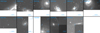 |
Fig. 5. VLT/FORS acquisition images of the SNe and their host galaxies (see Table 1). The light blue bars show the polarization angles of the ISP components. |
The above findings can be summarized as follows: the ISP of SN 2013ej and SN 2008bk should be dominated by MW components. The ISP of SN 2012ec and SN 2012dh might be dominated by MW components. The ISP of SN 2017gmr and SN 2010co might be affected by MW components. The ISP of SN 2017ahn, SN 2012aw, SN 2001du, and SN 2001dh likely originates mainly within their respective host galaxies.
5. Conclusions
In this paper, we have introduced a method for studying the ISP properties using 11 Type II SNe with a marginal ISP, in contrast to the previously studied objects with high extinctions and ISPs. One SN (SN 2010hv) shows zero ISP, while steady ISP components with ≲1.0% polarization degrees were observed in ten of the SNe in the sample. As for the wavelength dependence, SN 2001dh (and possibly also SN 2012aw) showed polarization maxima at short wavelengths (≲4000 Å), which is a similar property previously seen in several highly reddened SNe. The non-MW-like ISP in SN 2001dh and SN 2012aw likely originates from the IS dust in their host galaxies. The ISP in SN 2013ej showed a polarization maximum at a shorter wavelength than the average value of the MW ISP, but it is probably still within its diversity. This ISP likely originates from the IS dust in the MW. In the remaining seven SNe (SN 2017gmr, SN 2017ahn, SN 2012ec, SN 2012dh, SN 2010co, SN 2008bk, and SN 2001du), the uncertainties of the wavelength dependence are too large to determine whether the ISP is more similar to that seen in the MW or to that observed in some reddened SNe.
The investigation of the IS dust in external galaxies using the SN polarization has previously been limited mainly to highly reddened SNe, whose ISP dominates their polarization. The IS dust properties of only a few type II SNe have been investigated (SN 1999gi, SN 2022aau, and SN 2022ame; Leonard et al. 2001; Nagao et al. 2022). Our study increases the current SN sample available for investigating the IS dust in the host galaxies of Type II SNe, demonstrating that further investigation of a larger SN sample can provide new opportunities to study IS dust properties in external galaxies. In particular, the spectropolarimetry of SNe whose MW extinction is lower will be better suited for investigatations of the wavelength dependence of the ISP (i.e., the properties of the IS dust) in the SN host galaxies. In future work, it will be important to study the relations between the ISP properties and the global and local properties of the host galaxies in order to investigate the origin of the diverse properties of the IS dust in external galaxies.
In this work, the classification between Type IIP and IIL is based on the light-curve shapes of SNe, i.e. the decline rate during the photospheric phase (see follow-up paper Paper II for details).
NASA/IPAC Extragalactic Database.
SNOOPY is a collection of scripts, originally developed by F. Patat and later implemented in IRAF by E. Cappellaro. It is optimised for PSF-fitting photometry of point sources superimposed on a structured background.
Acknowledgments
We thank the anonymous referee for the comments, which substantially improved this paper. We are grateful to Stefan Taubenberger for the photometric and spectroscopic data of SN 2007aa and useful comments on the manuscript. We also thank Ferdinando Patat, Dietrich Baade, Aleksandar Cikota, Santiago González-Gaitán, Keiichi Maeda, Masaomi Tanaka and Mattia Bulla for useful discussions. This work is based on observations collected at the European Organisation for Astronomical Research in the Southern Hemisphere (ESO) under programmes 099.D-0543, 91.D-0401(A), 089.D-0515(A), 085.D-0391, 081.D-0128(A), 082.D-0151(A) and 67.D-0517(A). This research has made use of the services of the ESO Science Archive Facility. This work is based partly on observations collected at the Centro Astronómico Hispano en Andalucía (CAHA) at Calar Alto, operated jointly by Junta de Andalucía and Consejo Superior de Investigaciones Científicas (IAA-CSIC), under program F07_2.2_15. T.N. was funded by the Academy of Finland project 328898. H.K. was funded by the Academy of Finland projects 324504 and 328898. S.M. was funded by the Academy of Finland project 350458. This research has made use of NASA’s Astrophysics Data System Bibliographic Services.
References
- Anderson, J. P., González-Gaitán, S., Hamuy, M., et al. 2014, ApJ, 786, 67 [Google Scholar]
- Andrews, J. E., Sand, D. J., Valenti, S., et al. 2019, ApJ, 885, 43 [Google Scholar]
- Appenzeller, I., Fricke, K., Fürtig, W., et al. 1998, The Messenger, 94, 1 [NASA ADS] [Google Scholar]
- Barbarino, C., Dall’Ora, M., Botticella, M. T., et al. 2015, MNRAS, 448, 2312 [NASA ADS] [CrossRef] [Google Scholar]
- Beck, R. 2015, A&ARv, 24, 4 [Google Scholar]
- Bessell, M. S. 1990, PASP, 102, 1181 [NASA ADS] [CrossRef] [Google Scholar]
- Blondin, S., Modjaz, M., Kirshner, R., Challis, P., & Berlind, P. 2006, Cent. Bur. Electron. Telegrams, 757, 1 [NASA ADS] [Google Scholar]
- Bose, S., Kumar, B., Sutaria, F., et al. 2013, MNRAS, 433, 1871 [Google Scholar]
- Bose, S., Sutaria, F., Kumar, B., et al. 2015, ApJ, 806, 160 [Google Scholar]
- Brown, P. J., Breeveld, A. A., Holland, S., Kuin, P., & Pritchard, T. 2014, Ap&SS, 354, 89 [Google Scholar]
- Chassagne, R. 2001, IAU Circ., 7670, 3 [NASA ADS] [Google Scholar]
- Chornock, R., Filippenko, A. V., Branch, D., et al. 2006, PASP, 118, 722 [NASA ADS] [CrossRef] [Google Scholar]
- Chornock, R., Filippenko, A. V., Li, W., & Silverman, J. M. 2010, ApJ, 713, 1363 [Google Scholar]
- Chu, M. R., Cikota, A., Baade, D., et al. 2022, MNRAS, 509, 6028 [Google Scholar]
- Chugai, N. N., Fabrika, S. N., Sholukhova, O. N., et al. 2005, Astron. Lett., 31, 792 [NASA ADS] [CrossRef] [Google Scholar]
- Cikota, A., Hoang, T., Taubenberger, S., et al. 2018, A&A, 615, A42 [EDP Sciences] [Google Scholar]
- Dall’Ora, M., Botticella, M. T., Pumo, M. L., et al. 2014, ApJ, 787, 139 [CrossRef] [Google Scholar]
- Davis, L., Jr., & Greenstein, J. L. 1951, ApJ, 114, 206 [NASA ADS] [CrossRef] [Google Scholar]
- de Jaeger, T., Zheng, W., Stahl, B. E., et al. 2019, MNRAS, 490, 2799 [NASA ADS] [CrossRef] [Google Scholar]
- Deng, J. S., Cao, H. L., Xu, D. W., et al. 1999, IAU Circ., 7296, 3 [NASA ADS] [Google Scholar]
- Dessart, L., Leonard, D. C., John Hillier, D., & Pignata, G. 2021, A&A, 651, A19 [NASA ADS] [CrossRef] [EDP Sciences] [Google Scholar]
- Dhungana, G., Kehoe, R., Vinko, J., et al. 2016, ApJ, 822, 6 [NASA ADS] [CrossRef] [Google Scholar]
- Doi, T., Nakano, S., Itagaki, K., Naito, H., & Iizuka, R. 2007, Cent. Bur. Electron. Telegrams, 848, 1 [NASA ADS] [Google Scholar]
- Evans, R., Bock, G., Marples, P., et al. 2001, IAU Circ., 7690, 1 [NASA ADS] [Google Scholar]
- Fagotti, P., Dimai, A., Quadri, U., et al. 2012, Cent. Bur. Electron. Telegrams, 3054, 1 [NASA ADS] [Google Scholar]
- Folatelli, G., Gonzalez, S., & Morrell, N. 2007, Cent. Bur. Electron. Telegrams, 850, 1 [NASA ADS] [Google Scholar]
- Fraser, M., Kotak, R., Wright, D., et al. 2012, Cent. Bur. Electron. Telegrams, 3173, 1 [NASA ADS] [Google Scholar]
- Galbany, L., Hamuy, M., Phillips, M. M., et al. 2016, AJ, 151, 33 [NASA ADS] [CrossRef] [Google Scholar]
- Green, D. W. E. 2010, Cent. Bur. Electron. Telegrams, 2293, 2 [NASA ADS] [Google Scholar]
- Guillochon, J., Parrent, J., Kelley, L. Z., & Margutti, R. 2017, ApJ, 835, 64 [Google Scholar]
- Gutiérrez, C. P., Anderson, J. P., Hamuy, M., et al. 2017, ApJ, 850, 89 [CrossRef] [Google Scholar]
- Hosseinzadeh, G., Valenti, S., Arcavi, I., et al. 2017, ATel, 10059, 1 [NASA ADS] [Google Scholar]
- Howell, D. A., Höflich, P., Wang, L., & Wheeler, J. C. 2001, ApJ, 556, 302 [Google Scholar]
- Huang, F., Wang, X., Zhang, J., et al. 2015, ApJ, 807, 59 [Google Scholar]
- Inserra, C., Bulla, M., Sim, S. A., & Smartt, S. J. 2016, ApJ, 831, 79 [NASA ADS] [CrossRef] [Google Scholar]
- Itoh, R., Ui, T., & Yamanaka, M. 2012, Cent. Bur. Electron. Telegrams, 3054, 2 [NASA ADS] [Google Scholar]
- Jester, S., Schneider, D. P., Richards, G. T., et al. 2005, AJ, 130, 873 [Google Scholar]
- Kim, M., Zheng, W., Li, W., et al. 2013, Cent. Bur. Electron. Telegrams, 3606, 1 [NASA ADS] [Google Scholar]
- Koribalski, B. S., Staveley-Smith, L., Kilborn, V. A., et al. 2004, AJ, 128, 16 [Google Scholar]
- Leonard, D. C., Filippenko, A. V., Barth, A. J., & Matheson, T. 2000, ApJ, 536, 239 [Google Scholar]
- Leonard, D. C., Filippenko, A. V., Ardila, D. R., & Brotherton, M. S. 2001, ApJ, 553, 861 [NASA ADS] [CrossRef] [Google Scholar]
- Leonard, D. C., Filippenko, A. V., Chornock, R., & Foley, R. J. 2002a, PASP, 114, 1333 [NASA ADS] [CrossRef] [Google Scholar]
- Leonard, D. C., Filippenko, A. V., Gates, E. L., et al. 2002b, PASP, 114, 35 [Google Scholar]
- Leonard, D. C., Kanbur, S. M., Ngeow, C. C., & Tanvir, N. R. 2003, ApJ, 594, 247 [NASA ADS] [CrossRef] [Google Scholar]
- Leonard, D. C., Li, W., Filippenko, A. V., Foley, R. J., & Chornock, R. 2005, ApJ, 632, 450 [NASA ADS] [CrossRef] [Google Scholar]
- Leonard, D. C., Filippenko, A. V., Ganeshalingam, M., et al. 2006, Nature, 440, 505 [NASA ADS] [CrossRef] [Google Scholar]
- Leonard, D. C., Dessart, L., Hillier, D. J., & Pignata, G. 2012, AIP Conf. Ser., 1429, 204 [NASA ADS] [Google Scholar]
- Leonard, D. C., Dessart, L., Hillier, D. J., et al. 2021, ApJ, 921, L35 [NASA ADS] [CrossRef] [Google Scholar]
- Li, W. D. 1999, IAU Circ., 7294, 1 [NASA ADS] [Google Scholar]
- Li, W., Wang, X., Van Dyk, S. D., et al. 2007, ApJ, 661, 1013 [NASA ADS] [CrossRef] [Google Scholar]
- Lu, N. Y., Hoffman, G. L., Groff, T., Roos, T., & Lamphier, C. 1993, ApJS, 88, 383 [NASA ADS] [CrossRef] [Google Scholar]
- Mauerhan, J. C., Williams, G. G., Leonard, D. C., et al. 2015, MNRAS, 453, 4467 [CrossRef] [Google Scholar]
- Maza, J., Hamuy, M., Antezana, R., et al. 2012, Cent. Bur. Electron. Telegrams, 3163, 1 [NASA ADS] [Google Scholar]
- Monard, L. A. G. 2008, Cent. Bur. Electron. Telegrams, 1315, 1 [NASA ADS] [Google Scholar]
- Monard, L. A. G. 2010, Cent. Bur. Electron. Telegrams, 2271, 1 [NASA ADS] [Google Scholar]
- Monard, L. A. G., Childress, M., Scalzo, R., Yuan, F., & Schmidt, B. 2012, Cent. Bur. Electron. Telegrams, 3201, 1 [NASA ADS] [Google Scholar]
- Morrell, N. 2010, Cent. Bur. Electron. Telegrams, 2293, 1 [NASA ADS] [Google Scholar]
- Morrell, N., & Stritzinger, M. 2008, Cent. Bur. Electron. Telegrams, 1335, 1 [NASA ADS] [Google Scholar]
- Munari, U., Henden, A., Belligoli, R., et al. 2013, New A, 20, 30 [NASA ADS] [CrossRef] [Google Scholar]
- Nagao, T., Cikota, A., Patat, F., et al. 2019, MNRAS, 489, L69 [CrossRef] [Google Scholar]
- Nagao, T., Patat, F., Taubenberger, S., et al. 2021, MNRAS, 505, 3664 [NASA ADS] [CrossRef] [Google Scholar]
- Nagao, T., Patat, F., Maeda, K., et al. 2022, ApJ, 941, L4 [NASA ADS] [CrossRef] [Google Scholar]
- Nagao, T., Patat, F., Cikota, A., et al. 2023, ArXiv e-prints [arXiv:2308.00996] [Google Scholar]
- Nakano, S., Itagaki, K., Bouma, R. J., Lehky, M., & Hornoch, K. 2004, IAU Circ., 8377, 1 [NASA ADS] [Google Scholar]
- Nakano, S., Itagaki, K., & Kadota, K. 2006, Cent. Bur. Electron. Telegrams, 756, 1 [NASA ADS] [Google Scholar]
- Ntormousi, E. 2018, A&A, 619, L5 [NASA ADS] [CrossRef] [EDP Sciences] [Google Scholar]
- Patat, F., & Romaniello, M. 2006, PASP, 118, 146 [Google Scholar]
- Patat, F., Contreras, C., Prieto, J., et al. 2001, IAU Circ., 7680, 1 [NASA ADS] [Google Scholar]
- Patat, F., Benetti, S., Pastorello, A., Filippenko, A. V., & Aceituno, J. 2004, IAU Circ., 8378, 1 [NASA ADS] [Google Scholar]
- Patat, F., Höflich, P., Baade, D., et al. 2012, A&A, 545, A7 [NASA ADS] [CrossRef] [EDP Sciences] [Google Scholar]
- Patat, F., Taubenberger, S., Cox, N. L. J., et al. 2015, A&A, 577, A53 [NASA ADS] [CrossRef] [EDP Sciences] [Google Scholar]
- Pignata, G., Cifuentes, M., Maza, J., et al. 2010, Cent. Bur. Electron. Telegrams, 2456, 1 [NASA ADS] [Google Scholar]
- Poznanski, D., Nugent, P. E., Ofek, E. O., Gal-Yam, A., & Kasliwal, M. M. 2012, ATel, 3996, 1 [Google Scholar]
- Pursimo, T., Elias-Rosa, N., Dennefeld, M., et al. 2017, ATel, 10717, 1 [Google Scholar]
- Reilly, E., Maund, J. R., Baade, D., et al. 2017, MNRAS, 470, 1491 [NASA ADS] [CrossRef] [Google Scholar]
- Schlafly, E. F., & Finkbeiner, D. P. 2011, ApJ, 737, 103 [Google Scholar]
- Serkowski, K., Mathewson, D. S., & Ford, V. L. 1975, ApJ, 196, 261 [NASA ADS] [CrossRef] [Google Scholar]
- Shappee, B. J., Kochanek, C. S., Stanek, K. Z., et al. 2013, ATel, 5237, 1 [NASA ADS] [Google Scholar]
- Silverman, J. M., Foley, R. J., Filippenko, A. V., et al. 2012, MNRAS, 425, 1789 [Google Scholar]
- Smartt, S. J., Kilkenny, D., & Meikle, P. 2001, IAU Circ., 7704, 1 [NASA ADS] [Google Scholar]
- Smartt, S. J., Valenti, S., Fraser, M., et al. 2015, A&A, 579, A40 [NASA ADS] [CrossRef] [EDP Sciences] [Google Scholar]
- Sorce, J. G., Tully, R. B., Courtois, H. M., et al. 2014, MNRAS, 444, 527 [Google Scholar]
- Spiro, S., Pastorello, A., Pumo, M. L., et al. 2014, MNRAS, 439, 2873 [Google Scholar]
- Springob, C. M., Masters, K. L., Haynes, M. P., Giovanelli, R., & Marinoni, C. 2009, ApJS, 182, 474 [NASA ADS] [CrossRef] [Google Scholar]
- Stevance, H. F., Maund, J. R., Baade, D., et al. 2017, MNRAS, 469, 1897 [NASA ADS] [CrossRef] [Google Scholar]
- Stevance, H. F., Maund, J. R., Baade, D., et al. 2019, MNRAS, 485, 102 [NASA ADS] [CrossRef] [Google Scholar]
- Stritzinger, M., Hamuy, M., Suntzeff, N. B., et al. 2002, AJ, 124, 2100 [NASA ADS] [CrossRef] [Google Scholar]
- Takaki, K., Moritani, Y., Itoh, R., et al. 2012, Cent. Bur. Electron. Telegrams, 3203, 1 [NASA ADS] [Google Scholar]
- Takáts, K., & Vinkó, J. 2012, MNRAS, 419, 2783 [CrossRef] [Google Scholar]
- Tartaglia, L., Sand, D., Valenti, S., et al. 2017, ATel, 10058, 1 [NASA ADS] [Google Scholar]
- Tartaglia, L., Sand, D. J., Valenti, S., et al. 2018, ApJ, 853, 62 [Google Scholar]
- Tartaglia, L., Sand, D. J., Groh, J. H., et al. 2021, ApJ, 907, 52 [NASA ADS] [CrossRef] [Google Scholar]
- Tody, D. 1986, SPIE Conf. Ser., 627, 733 [Google Scholar]
- Tody, D. 1993, ASP Conf. Ser., 52, 173 [NASA ADS] [Google Scholar]
- Trammell, S. R., Hines, D. C., & Wheeler, J. C. 1993, ApJ, 414, L21 [NASA ADS] [CrossRef] [Google Scholar]
- Tran, H. D., Filippenko, A. V., Schmidt, G. D., et al. 1997, PASP, 109, 489 [CrossRef] [Google Scholar]
- Tsvetkov, D. Y., Goranskij, V., & Pavlyuk, N. 2008, Peremennye Zvezdy, 28, 8 [NASA ADS] [Google Scholar]
- Tully, R. B., Courtois, H. M., Dolphin, A. E., et al. 2013, AJ, 146, 86 [NASA ADS] [CrossRef] [Google Scholar]
- Tully, R. B., Courtois, H. M., & Sorce, J. G. 2016, AJ, 152, 50 [Google Scholar]
- Valenti, S., Tartaglia, L., Sand, D., et al. 2017, ATel, 10706, 1 [NASA ADS] [Google Scholar]
- Van Dyk, S. D., Davidge, T. J., Elias-Rosa, N., et al. 2012a, AJ, 143, 19 [NASA ADS] [CrossRef] [Google Scholar]
- Van Dyk, S. D., Cenko, S. B., Poznanski, D., et al. 2012b, ApJ, 756, 131 [NASA ADS] [CrossRef] [Google Scholar]
- Vinkó, J., Takáts, K., Sárneczky, K., et al. 2006, MNRAS, 369, 1780 [CrossRef] [Google Scholar]
- Wang, L., & Wheeler, J. C. 2008, ARA&A, 46, 433 [Google Scholar]
- Wang, L., Wheeler, J. C., & Höflich, P. 1997, ApJ, 476, L27 [NASA ADS] [CrossRef] [Google Scholar]
- Wang, L., Howell, D. A., Höflich, P., & Wheeler, J. C. 2001, ApJ, 550, 1030 [NASA ADS] [CrossRef] [Google Scholar]
- Whittet, D. C. B., Martin, P. G., Hough, J. H., et al. 1992, ApJ, 386, 562 [NASA ADS] [CrossRef] [Google Scholar]
- Zelaya, P., Clocchiatti, A., Baade, D., et al. 2017, ApJ, 836, 88 [NASA ADS] [CrossRef] [Google Scholar]
- Zgirski, B., Gieren, W., Pietrzyński, G., et al. 2017, ApJ, 847, 88 [Google Scholar]
Appendix A: Observation logs
The observation logs for the spectropolarimetric data are shown here.
Log of the observations of SN 2017gmr. The observations were made under the program ID 099.D-0543.
Log of the observations of SN 2017ahn. The observations were made under the program ID 099.D-0543.
Log of the observations of SN 2013ej. The observations were made under the program ID 091.D-0401(A).
Log of the observations of SN 2012ec. The observations were made under the program ID 089.D-0515(A).
Log of the observations of SN 2012dh. The observations were made under the program ID 089.D-0515(A).
Log of the observations of SN 2012aw. The observations were made under the program ID 089.D-0515(A).
Log of the observations of SN 2010hv. The observations were made under the program ID 085.D-0391.
Log of the observations of SN 2010co. The observations were made under the program ID 085.D-0391.
Log of the observations of SN 2008bk. The observations were made under the program IDs 081.D-0128(A) and 082.D-0151(A).
Log of the observations of SN 2001du. The observations were made under the program ID 67.D-0517(A).
Log of the observations of SN 2001dh. The observations were made under the program ID 67.D-0517(A).
Appendix B: SN 2007aa
B.1. Photometry
We obtained UBVRI-band images of SN 2007aa with the CAFOS (Calar Alto Faint Object Spectrograph) instrument, the visual imager and low-resolution spectrograph at the Calar Alto 2.2m Telescope. All frames were de-biased and flatfield-corrected using standard techniques with IRAF. Bessell (1990) magnitudes of local field stars were derived from their Sloan ugri magnitudes reported in the SDSS catalogue using the transformation equations by Jester et al. (2005). Instrumental SN magnitudes were measured through PSF photometry with SNOOPY5, subtracting a local fit to the underlying host-galaxy light. The instrumental SN magnitudes were then calibrated to the Bessell (1990) system with zero points obtained from the local sequence stars and S-corrections (Stritzinger et al. 2002) calculated with the help of the spectra described in Section B.2. Photometric uncertainties were estimated as the quadratic sum of PSF-fitting uncertainties, uncertainties in the PSF-to-aperture correction, uncertainties in the photometric zero points, and uncertainties in the background fit estimated through an artificial-star experiment. In reality, these contributions may not be fully independent, hence our errors might be over-estimated in some cases. The resulting S-corrected photometry along with the derived uncertainties is provided in Figure B.1 and Table B.1.
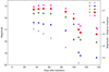 |
Fig. B.1. Photometry of SN 2007aa. The assumed explosion date is 54 126.7 MJD. |
Photometry of SN 2007aa
B.2. Spectroscopy
We also obtained optical spectroscopy of SN 2007aa with the CAFOS instrument at the Calar Alto 2.2m Telescope, using the b200 and r200 grisms, and a 1.5" slit aligned along the parallactic angle to minimise differential slit losses. After the usual de-biasing and flatfielding, a variance-weighted extraction of the spectra was performed in the IRAF task APALL. The wavelength solution was established with the help of arc-lamp spectra and checked against night-sky emission lines. The flux calibration was performed with the help of sensitivity curves derived from standard-star observations. b200 and r200 spectra obtained during the same night were combined to increase the wavelength coverage and the S/N in the overlap region. All spectra were corrected for telluric absorptions on a best-effort basis. As a final step, the flux of the spectra was checked against the contemporaneous BVRI photometry (Section B.1) and adjusted with linear functions if necessary. A log of the spectroscopic observations is reported in Table B.2. The spectra are shown in Figure B.2.
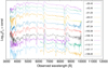 |
Fig. B.2. Spectra of SN 2007aa. The days after the assumed explosion date (54 126.7 MJD) are shown. |
Log of the spectroscopy of SN 2007aa.
Appendix C: Spectroscopic data of the FORS/VLT sample
The spectra obtained as the spectropolarimetric observations for the VLT sample are provided here. All the spectra are normalized by their continuum flux using the IRAF onedspec.continuum task with the cubic spline curve and the rejection limit of 2 residual sigma.
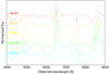 |
Fig. C.1. FORS spectrum of SN 2017gmr. The top-left number in each panel shows the phase of the spectrum (days relative to end of the photospheric phase; see Paper II). |
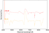 |
Fig. C.10. Same as Figure C.1, but for SN 2001du. |
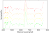 |
Fig. C.11. Same as Figure C.1, but for SN 2001dh. |
Appendix D: Polarization spectra
The polarization spectra of all the SNe before ISP subtraction are shown here. In order to increase the signal-to-noise ratio, the spectra have been rebinned to 25-Å bins here.
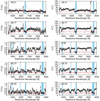 |
Fig. D.1. Polarization degree (left) and angle (right) of SN 2017gmr before the ISP subtraction at different epochs (increasing from the top to the bottom as labelled). The grey lines in the background of each plot are the unbinned flux spectra at the same epochs. The blue shading shows the adopted wavelength ranges for the emission lines at each epoch. The red lines show the best-fit ISP. The top-left number in each panel shows the phase (days relative to end of the photospheric phase; see Paper II). |
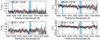 |
Fig. D.10. Same as Fig. D.1, but for SN 2001du. |
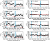 |
Fig. D.11. Same as Fig. D.1, but for SN 2001dh. |
Appendix E: Extracted ISP components
The extracted ISP components for all the SNe are shown here.
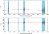 |
Fig. E.1. Polarization degree P and angle θ selected for the ISP in SN 2017ahn. The red lines and the blue shading are the same as in Fig. 2. |
All Tables
Log of the observations of SN 2017gmr. The observations were made under the program ID 099.D-0543.
Log of the observations of SN 2017ahn. The observations were made under the program ID 099.D-0543.
Log of the observations of SN 2013ej. The observations were made under the program ID 091.D-0401(A).
Log of the observations of SN 2012ec. The observations were made under the program ID 089.D-0515(A).
Log of the observations of SN 2012dh. The observations were made under the program ID 089.D-0515(A).
Log of the observations of SN 2012aw. The observations were made under the program ID 089.D-0515(A).
Log of the observations of SN 2010hv. The observations were made under the program ID 085.D-0391.
Log of the observations of SN 2010co. The observations were made under the program ID 085.D-0391.
Log of the observations of SN 2008bk. The observations were made under the program IDs 081.D-0128(A) and 082.D-0151(A).
Log of the observations of SN 2001du. The observations were made under the program ID 67.D-0517(A).
Log of the observations of SN 2001dh. The observations were made under the program ID 67.D-0517(A).
All Figures
|
Fig. 1. Polarization degree P (top panel) and angle θ (bottom panel) for SN 2017gmr at five different epochs: 58045.60, 58067.24, 58099.86, 58108.76, and 58 134.93 (MJD; purple, green, sky-blue, orange, and yellow symbols, respectively). The data are binned to 5 Å. The gray lines at the bottom of each plot represent the total-flux spectra on 58 134.93 (MJD). The red lines show the polarization degree and angle of the ISP as approximated by P(λ) = Pmaxexp[−Kln2(λmax/λ)] with fixed values of Pmax = 0.35, λmax = 6400 Å and K = 4.0, and θISP = 33.37. The blue shading shows the wavelength windows at the adopted lines, where at all epochs the flux was > 1.1 times higher than in the nearby continuum regions. |
| In the text | |
|
Fig. 2. Polarization degree P (top panel) and angle θ (bottom panel) selected for the determination of the ISP in SN 2017gmr. The red lines and the blue-shaded areas are the same as in Fig. 1. In each wavelength bin, the ISP values are the average over all five epochs, after removal of outliers as described in Sect. 4.1. The red lines show the best-fit ISP from Sect. 4.1 and Table 4. |
| In the text | |
|
Fig. 3. ISP λmax–K diagram for the Type II SNe in this study. Several Type Ia SNe (black crosses; Patat et al. 2015; Zelaya et al. 2017; Cikota et al. 2018) and a large number of MW stars (gray crosses; Whittet et al. 1992) are also included. The colored points show the best-fit values of the Type II SNe, and the lines represent the 1σ confidence intervals for the fitting. |
| In the text | |
|
Fig. 4. Wavelength dependence of the ISP (normalized to the polarization at 4000 Å) toward SN 2013ej, SN 2012aw, and SN 2001dh (colored points) with their Serkowski law best fits (colored lines). For comparison, the data of three Type Ia SNe (SN 2014J, SN 2008fp, and SN 2006X; Patat et al. 2015) and a Galactic star (HD 43384; Cikota et al. 2018) are also plotted. |
| In the text | |
|
Fig. 5. VLT/FORS acquisition images of the SNe and their host galaxies (see Table 1). The light blue bars show the polarization angles of the ISP components. |
| In the text | |
|
Fig. B.1. Photometry of SN 2007aa. The assumed explosion date is 54 126.7 MJD. |
| In the text | |
|
Fig. B.2. Spectra of SN 2007aa. The days after the assumed explosion date (54 126.7 MJD) are shown. |
| In the text | |
|
Fig. C.1. FORS spectrum of SN 2017gmr. The top-left number in each panel shows the phase of the spectrum (days relative to end of the photospheric phase; see Paper II). |
| In the text | |
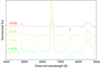 |
Fig. C.2. Same as Figure C.1, but for SN 2017ahn. |
| In the text | |
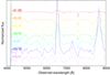 |
Fig. C.3. Same as Figure C.1, but for SN 2013ej. |
| In the text | |
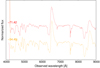 |
Fig. C.4. Same as Figure C.1, but for SN 2012ec. |
| In the text | |
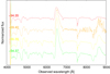 |
Fig. C.5. Same as Figure C.1, but for SN 2012dh. |
| In the text | |
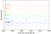 |
Fig. C.6. Same as Figure C.1, but for SN 2012aw. |
| In the text | |
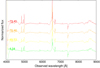 |
Fig. C.7. Same as Figure C.1, but for SN 2010hv. |
| In the text | |
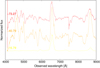 |
Fig. C.8. Same as Figure C.1, but for SN 2010co. |
| In the text | |
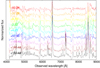 |
Fig. C.9. Same as Figure C.1, but for SN 2008bk. |
| In the text | |
|
Fig. C.10. Same as Figure C.1, but for SN 2001du. |
| In the text | |
|
Fig. C.11. Same as Figure C.1, but for SN 2001dh. |
| In the text | |
|
Fig. D.1. Polarization degree (left) and angle (right) of SN 2017gmr before the ISP subtraction at different epochs (increasing from the top to the bottom as labelled). The grey lines in the background of each plot are the unbinned flux spectra at the same epochs. The blue shading shows the adopted wavelength ranges for the emission lines at each epoch. The red lines show the best-fit ISP. The top-left number in each panel shows the phase (days relative to end of the photospheric phase; see Paper II). |
| In the text | |
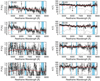 |
Fig. D.2. Same as Fig. D.1, but for SN 2017ahn. |
| In the text | |
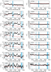 |
Fig. D.3. Same as Fig. D.1, but for SN 2013ej. |
| In the text | |
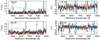 |
Fig. D.4. Same as Fig. D.1, but for SN 2012ec. |
| In the text | |
 |
Fig. D.5. Same as Fig. D.1, but for SN 2012dh. |
| In the text | |
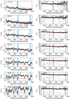 |
Fig. D.6. Same as Fig. D.1, but for SN 2012aw. |
| In the text | |
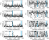 |
Fig. D.7. Same as Fig. D.1, but for SN 2010hv. |
| In the text | |
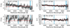 |
Fig. D.8. Same as Fig. D.1, but for SN 2010co. |
| In the text | |
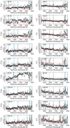 |
Fig. D.9. Same as Fig. D.1, but for SN 2008bk. |
| In the text | |
|
Fig. D.10. Same as Fig. D.1, but for SN 2001du. |
| In the text | |
|
Fig. D.11. Same as Fig. D.1, but for SN 2001dh. |
| In the text | |
|
Fig. E.1. Polarization degree P and angle θ selected for the ISP in SN 2017ahn. The red lines and the blue shading are the same as in Fig. 2. |
| In the text | |
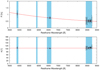 |
Fig. E.2. Same as Fig. E.1, but for SN 2013ej. |
| In the text | |
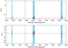 |
Fig. E.3. Same as Fig. E.1, but for SN 2012ec. |
| In the text | |
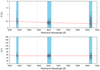 |
Fig. E.4. Same as Fig. E.1, but for SN 2012dh. |
| In the text | |
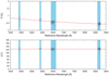 |
Fig. E.5. Same as Fig. E.1, but for SN 2012aw. |
| In the text | |
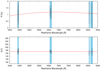 |
Fig. E.6. Same as Fig. E.1, but for SN 2010co. |
| In the text | |
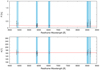 |
Fig. E.7. Same as Fig. E.1, but for SN 2008bk. |
| In the text | |
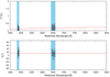 |
Fig. E.8. Same as Fig. E.1, but for SN 2001du. |
| In the text | |
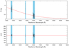 |
Fig. E.9. Same as Fig. E.1, but for SN 2001dh. |
| In the text | |
Current usage metrics show cumulative count of Article Views (full-text article views including HTML views, PDF and ePub downloads, according to the available data) and Abstracts Views on Vision4Press platform.
Data correspond to usage on the plateform after 2015. The current usage metrics is available 48-96 hours after online publication and is updated daily on week days.
Initial download of the metrics may take a while.