| Issue |
A&A
Volume 629, September 2019
|
|
|---|---|---|
| Article Number | A143 | |
| Number of page(s) | 26 | |
| Section | Cosmology (including clusters of galaxies) | |
| DOI | https://doi.org/10.1051/0004-6361/201935676 | |
| Published online | 19 September 2019 | |
Towards mapping turbulence in the intra-cluster medium
I. Sample variance in spatially-resolved X-ray line diagnostics
1
IRAP, Université de Toulouse, CNRS, UPS, CNES, Toulouse, France
e-mail: This email address is being protected from spambots. You need JavaScript enabled to view it.
2
CNES, 18 Avenue Edouard Belin, 31400 Toulouse, France
Received:
12
April
2019
Accepted:
22
July
2019
Abstract
Context. X-ray observations of galaxy clusters provide insights into the nature of gaseous turbulent motions, their physical scales, and the fundamental processes to which they are related. Spatially-resolved, high-resolution spectral measurements of X-ray emission lines provide diagnostics on the nature of turbulent motions in emitting atmospheres. Since they are acting on scales comparable to the size of the objects, the uncertainty on these physical parameters is limited by the number of observational measurements, through sample variance.
Aims. We propose a different and complementary approach to repeating numerical simulations for the computation of sample variance (i.e. Monte-Carlo sampling) by introducing new analytical developments for lines diagnosis.
Methods. We considered the model of a “turbulent gas cloud”, consisting in isotropic and uniform turbulence described by a universal Kolmogorov power-spectrum with random amplitudes and phases in an optically thin medium. Following a simple prescription for the four-term correlation of Fourier coefficients, we derived generic expressions for the sample mean and variance of line centroid shift, line broadening, and projected velocity structure function. We performed a numerical validation based on Monte-Carlo simulations for two popular models of gas emissivity based on the β-model.
Results. Generic expressions for the sample variance of line centroid shifts and broadening in arbitrary apertures are derived and match the simulations within their range of applicability. Generic expressions for the mean and variance of the structure function are provided and verified against simulations. An application to the Athena/X-IFU (Advanced Telescope for High-ENergy Astrophysics/X-ray Integral Field Unit) and XRISM/Resolve (X-ray Imaging and Spectroscopy Mission) instruments forecasts the potential of sensitive, spatially-resolved spectroscopy to probe the inertial range of turbulent velocity cascades in a Coma-like galaxy cluster.
Conclusions. The formulas provided are of generic relevance and can be implemented in forecasts for upcoming or current X-ray instrumentation and observing programmes.
Key words: galaxies: clusters: intracluster medium / line: profiles / methods: analytical / turbulence / X-rays: galaxies: clusters / techniques: imaging spectroscopy
© N. Clerc et al. 2019
 Open Access article, published by EDP Sciences, under the terms of the Creative Commons Attribution License (http://creativecommons.org/licenses/by/4.0), which permits unrestricted use, distribution, and reproduction in any medium, provided the original work is properly cited.
1. Introduction
Galaxy clusters form by accretion of matter along filaments of the cosmic web, either continuously or episodically through major and minor merger events. The baryonic gas flowing along filamentary structures and falling into their deep gravitational wells acquires kinetic energy that is transformed into thermal energy, magnetic field amplification, and cosmic ray acceleration in the intra-cluster medium, by a succession of shocks, large-scale motions, and dissipation by turbulent processes (Ryu et al. 2008; Zhuravleva et al. 2014; Gaspari et al. 2014, 2018; Miniati & Beresnyak 2015; Vazza et al. 2018). Observational signatures of these phenomena are rare and difficult to obtain. The most promising and efficient diagnostics are issued from spectroscopic observations of the hot intra-cluster gas, which permeates the entire volume of massive halos and emits copious amounts of X-ray light.
Focusing mainly on X-ray emission lines extracted along a single line of sight, Inogamov & Sunyaev (2003) demonstrated that departures from Gaussian line shapes carry important indications on the nature of large-scale turbulence in the intra-cluster medium. The authors extended their formula to two-dimensional diagnostics by introducing the correlation function of the projected velocity field and calculating its scaling relative to fundamental parameters such as the turbulent injection and dissipation scales. Applying these findings to simple but realistic configurations of the intra-cluster medium, Zhuravleva et al. (2012) calculated exact expressions for emission line diagnostics such as centroid shift, broadening, and two-dimensional correlation function. They evaluated the associated sampling uncertainty (also called “sample variance” or “sampling variance”) by multiple Monte-Carlo realisations of the velocity field and showed that it can dominate the overall error budget in the presence of large-scale turbulence. ZuHone et al. (2016) were able to evaluate the contribution of sample variance and statistical errors for the well-defined observational case of the Coma cluster, thereby demonstrating the impact of the observational strategy on this source of uncertainty. Using numerically simulated clusters instead, Roncarelli et al. (2018) performed end-to-end simulations to derive expected values of the indicators of turbulence issued from emission line measurements, postponing the calculation of sample variance to a later stage by means of multiple realisations.
In this work we propose a formal approach to the problem of sample variance by considering the ideal case of an arbitrary, optically-thin gas distribution in which uniform and isotropic turbulent motions take place. This study is motivated by the intent to obtain reliable and fast estimates of this specific class of uncertainties and to identify key parameters that have an impact upon them. We will consider three popular diagnostics extracted from a continuum-free, isolated spectral line in the X-ray wavebands: line centroid shift (hereafter C), line broadening (S), and projected velocity structure function (SF). The latter is defined as the squared difference of projected velocities averaged amongst all points separated by a distance s on sky. Instrumental characteristics and signal-to-noise considerations, related for example to the exposure time or the energy resolution, are deliberately excluded and addressed in a separate work (Cucchetti et al. 2019, hereafter Paper II) The results of the present work are therefore instrument-independent to some extent.
Amongst these indicators, the structure function appears as a very promising diagnostic of turbulence since it takes advantage of spatially-resolved spectroscopic observations, as enabled by integral field units. It is also the least intuitive of all three diagnostics. Effects such as heterogenous sampling, non-stationarity, and anisotropies reflect diversely in the modelling of SF. Interestingly, the structure function as a mathematical tool has received extensive interest in multiple fields of research involving spatial statistics, notably geostatistics and Earth science, under the name “variogram” (e.g. Matheron 1965, 1973; Cressie 1985; Haslett 1997; Armstrong 1998; Corstanje et al. 2008). In the field of astronomy and astrophysics where its use is comparatively less widespread, it is involved in various works under both of the terms “structure function” and “variogram”, to analyse data either in one dimension (e.g. Roelens et al. 2017, for stellar variability), two (e.g. Cayón 2010, for cosmic microwave background), or three and more dimensions (e.g. Martínez et al. 2010, for galaxy clustering).
We first introduce the derivation of the average and variance of the centroid shift and line broadening for measurements of an X-ray spectral line along a single line of sight, together with a numerical validation (Sect. 2). Section 3 generalises these results to the case of three-dimensional turbulent fields and the extension of the line diagnostics to two dimensions, thereby treating the case of the structure function. We perform a numerical validation of these results in Sect. 4. We finally discuss our results in Sect. 5 and highlight two specific cases matching the future X-ray instruments XRISM/Resolve (X-ray Imaging and Spectroscopy Mission, Ishisaki et al. 2018) and Athena/X-IFU (Advanced Telescope for High-ENergy Astrophysics/X-ray Integral Field Unit, Barret et al. 2016, 2018). We report most of the details on calculations and their discussions in the appendices, to which the reader can refer for more details.
The convention in our notations is as follows: the line-of-sight direction is denoted by x and the plane-of-sky coordinate is θ = (y, z). Units of these coordinates are physical (kiloparsec) since in practice the angular distance at the redshift of the object is known. Three-dimensional vectors are underlined to differentiate them from two-dimensional vectors. The velocity v (units of km s−1) is the component of the gas velocity projected along the line of sight. All following definitions and derivations (e.g. turbulent velocity dispersion, power-spectrum, etc.) are relative to this line-of-sight component. We denote with brackets ⟨.⟩ the sample average of the estimators and random variables. We will decompose the velocity field in Fourier coefficients with discrete indices (involving the discrete summation sign ∑k). The emissivity and geometrical shapes will be treated with their continuous Fourier transforms (involving the continuous summation sign ∫dk). This distinction will often be purely formal: we made this choice to clarify the calculations. One- and three-dimensional Fourier transforms are indicated with a tilde (e.g.  ), two-dimensional transforms with a hat (e.g.
  ).
).
2. Measured velocity dispersion along single line of sight
In this section we assume the velocity structure diagnostics are issued from the measurement of an emission line profile (e.g. iron XXV at ∼6.5 keV) along a given line of sight. Measuring a line profile is a complex task involving tools and methods developed under a certain set of observational conditions (binning of the spectra, level of noise, background subtraction, continuum subtraction etc.) In order to illustrate our findings, we adopt a simplified approach where the analysis applies to a continuum- and background-subtracted spectrum with no source of noise or uncertainty and no systematic (corresponding to a virtually infinite exposure time with a perfectly calibrated instrument). Only one emission line is investigated, thus we neglect blending with neighbouring lines. Importantly, we do not provide a prescription for the measurement process itself (Gaussian or more complex fit, non-parametric fit, full spectrum fitting, etc.) Instead we model such a measurement as a calculation of the zero-th, first, and second moments of the line energy distribution Il(E) integrated along a line of sight θ0, such that
where δE and Σ are the observed centroid shift (relative to reference energy E0) and width (or broadening) of the line, and F is a normalisation factor, namely the flux in the line. We introduce the gas velocity field along the line of sight fixed by θ0 with v(x) ≡ v(x, θ0). We define C = cδE/E0 and  as the observed centroid shift and width in velocity space.
2.1. Emission along the line of sight
At a microscopic level (i.e. below the turbulent dissipation scale in the medium), emission is assumed to follow a thermally broadened line profile. We neglect any additional broadening such as natural (Lorentzian) and assign each ion a rest-frame Gaussian emission profile. Assuming a purely collisional origin of the emission line, the amplitude of the line is assumed to scale with emissivity  . The coefficient of proportionality may depend on the local property of the medium (metallicity, temperature, etc.)
In the following we assume that the turbulent dissipation scale Ldiss is large enough for each volume of size (Ldiss)3 to contain a significantly large number of line emitters: it is practically always fulfilled, even for the tenuous intra-cluster medium with a typical density of 10−3 cm−3 and kiloparsec-scale injection scales. Accounting for the Doppler shift in energy v(x)/c and emissivity ϵ(x), we therefore model the total emission at each point by
![Mathematical equation: $$ \begin{aligned} \frac{\mathrm{d} I_{l}(E)}{\mathrm{d} x} = \frac{\epsilon (x) c}{E_0\sigma _{\rm th}(x) \sqrt{2 \pi }} \exp \left( -\frac{1}{2} \left[\frac{E-E_0 (1+v(x)/c)}{E_0 \sigma _{\rm th}(x)/c}\right]^2 \right)\cdot \end{aligned} $$](/articles/aa/full_html/2019/09/aa35676-19/aa35676-19-eq6.gif) (1)
(1)
Assuming an optically thin medium and reordering the summation over velocities, we can write
![Mathematical equation: $$ \begin{aligned}&F({\boldsymbol{\theta }}_0) = \int \epsilon (x) \mathrm{d} x \nonumber \\&C({\boldsymbol{\theta }}_0) = F^{-1} \int \epsilon (x) v(x) \mathrm{d} x \nonumber \\&S^2({\boldsymbol{\theta }}_0) = F^{-1} \int \epsilon (x) \sigma _{\rm th}^2(x) \mathrm{d} x + \frac{F^{-2}}{2} \int \int G(x,x^{\prime }) \mathrm{d} x \mathrm{d} x^{\prime } \\&G(x,x^{\prime }) = \epsilon (x) \epsilon (x^{\prime }) \left[v(x)-v(x^{\prime })\right]^2.\nonumber \end{aligned} $$](/articles/aa/full_html/2019/09/aa35676-19/aa35676-19-eq7.gif) (2)
(2)
These integrals extend along the line of sight indexed by x, which we assume to range in a large interval [ − L, L]. In principle v(x) encapsulates the effect of hydrodynamical motions (turbulence) and bulk motions of the gas. Without loss of generality, we assume bulk motions over a small area are known and subtracted from the measurements; we therefore set its contribution to zero.
2.2. Turbulent velocity field
We describe the turbulent velocity field v by its Fourier series expansion, with positive and negative values of k:
The coefficients Vk are complex random variables, defined as  . Here ψk is a random phase and |Vk| a random modulus, supposedly independent from each other. In the following, we define for convenience ω = 2π/L. We note that ⟨v⟩=0, leading to V0 = 0. Averaging over multiple random realisations provides
 (3)
(3)
where P(k)=P(−k)=⟨|Vk|2⟩ is the power spectrum of the turbulent velocity field and δij = 1 if i = j, 0 if i ≠ j.
Our hypothesis of uniform turbulence implies that the normalisation of the power spectrum matches the square of the turbulent velocity dispersion σturb at any given point x. It is defined through the calculation of the second moment  , where averaging occurs over random phases and moduli. Therefore (taking e.g. x = 0),
  . This definition does not involve the profile of the emissivity, in contrast for example to ZuHone et al. (2016).
One simple assumption for the distribution of moduli (e.g. Inogamov & Sunyaev 2003) consists in non-random coefficients, leaving only phases as random. Another popular and physically-motivated assumption (although not systematically required in the rest of this paper) is the Rayleigh distribution (e.g. ZuHone et al. 2016),
which reflects the fact that the turbulent velocity is a Gaussian random field. Introducing Rk = P(k)2 − Var(|Vk|2), we obtain, under the assumption of Rayleigh-distributed moduli, Rk = 0 for all k.
2.3. Statistics of the centroid shift and line broadening
Calculations in Appendix A provide the following formulas for the centroid shift:
 (4)
(4)
and its variance
 (5)
(5)
This expression is identical to Eq. (A9) in Zhuravleva et al. (2012), since  is the Fourier power spectrum of the (unnormalised, one-dimensional) emissivity ϵ.
As for the line broadening, in Appendix A we obtain
 (6)
(6)
The horizontal bar denotes averaging of the thermal component along the line of sight. Again this expression is similar to Eq. (B4) in Zhuravleva et al. (2012). Also interesting is the contribution of the last term, indicating that averaging many (independent) measurements of broadening measurements generally provides a biased estimate of the (thermal plus turbulent) broadening. The bias is zero only in cases where the turbulent power spectrum and the emissivity power spectrum act on distinct spatial scales. Finally, the variance can be written as
![Mathematical equation: $$ \begin{aligned} \mathrm{Var} (S^2)=&2 \sum _{j,k} P(k) P(j) \left| \frac{\widetilde{\epsilon }(j+k)}{F}-\frac{\widetilde{\epsilon }(j) \widetilde{\epsilon }(k)}{F^2} \right|^2 \nonumber \\&- \sum _k R_k \times \left\{ \left| \frac{\widetilde{\epsilon }(2k)}{F} - \frac{\widetilde{\epsilon }(k)^2}{F^2} \right|^2 + 2 \left[ 1-\frac{P_{\epsilon }(k)}{F^2} \right]^2 \right\} \cdot \end{aligned} $$](/articles/aa/full_html/2019/09/aa35676-19/aa35676-19-eq18.gif) (7)
(7)
Conveniently, if the moduli |Vk| are Rayleigh distributed, the term under the second k-sum vanishes.
2.4. Numerical validation
A verification of the equations previously derived is a relatively quick task with modern computing resources. We considered a power spectrum in the form P(k)∝1/k2α + 1 in the inertial range [kmin, kmax] and zero outside of it. The slope is α = 1/3. We simulated the line profile resulting from the projection through a (isothermal, isometallic) β-model density profile (Cavaliere & Fusco-Femiano 1978) with β = 2/3, core-radius rc, and distance θ to the cluster centre:
where L = 2, rc = 0.2, and θ = 0.2. The moduli Vk may be constant (non-random) or follow a Rayleigh distribution. The Fourier coefficients of the emissivity are given by ZuHone et al. (2016) (see also Appendix B):  with
with  . An example of such a realisation is shown in Fig. 1. Only phases are random in this illustration. This configuration and random realisation are specifically chosen to highlight the possible discrepancy between the value of the broadening S2 and the simple estimate
  . Indeed, purely by chance, most of the points where velocity is high are located in low-emissivity regions, therefore their contribution to line broadening is weak.
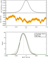 |
Fig. 1. One realisation of a uni-dimensional turbulent velocity field (middle panel) along the spatial axis x (in arbitrary units) with parameters α = 1/3, kmin = 1 (Linj = 2), kmax = 20 (Ldiss = 0.1), σturb = 160 km s−1, and σth = 100 km s−1 (shown by yellow shading). The emissivity profile (top panel) of the gas corresponds to a β density model with core radius rc = 0.2 and at a distance θ = 0.2 from the centre. The lower panel shows the resulting line profile as a thick black line. The best-fit Gaussian centred on C (vertical line) of width S is shown as a dashed red line. The green thin curve shows the Gaussian centred on the line centroid. Its width equals the geometrical mean of the thermal and turbulent broadening. |
Figure 2 shows the excellent agreement between the theoretical and simulated quantities after 5000 random realisations of the velocity field. It is important to notice the strong non-gaussianity of S2 and C in general. The configuration chosen for this simulation clearly illustrates that  . This is a consequence of the injection scale (Linj ∼ L) being much larger than the typical cluster characteristic scale (here rc = L/10), leading to non-Gaussian line shapes (Inogamov & Sunyaev 2003).
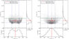 |
Fig. 2. Line centroid C versus line width (squared) S2 of an emission line along a single line of sight and 5000 realisations of a one-dimensional turbulent velocity field (σturb = 160 km s−1, kmin = 1, kmax = 20, σth = 100 km s−1). Left panel: assumes only random phases while the right panel also includes randomly distributed moduli (Rayleigh distribution). Points show measurements, and the red cross is the measured mean and standard deviations along both axes. The blue lines represent the results obtained from analytical calculations (Eqs. (4)–(7)). The plain green line shows the location of the geometric mean of the turbulent and thermal dispersions: the presence of turbulent motions on scales comparable to that of the cluster makes such an estimate a biased one. |
3. Two-dimensional characterisation of the velocity field
Observations and diagnostics of the intra-cluster medium rarely rely on single-line-of-sight measurements. Instead, due to instrumental resolution limits and signal-to-noise considerations, line centroid shifts and broadening are measured from spectra collected over well-defined two-dimensional regions, sometimes denoted as “bins” or “pixels”. A popular diagnostic tool in the field of astrophysical turbulence (e.g. Lis et al. 1998; Esquivel et al. 2007; Anorve-Zeferino 2019) is the two-dimensional structure function, loosely speaking a 2D correlation function analysis of the line centroid shift map. Obtaining analytical expressions of the sample variance of these estimators requires the formalism above to be extended and to account for the three-dimensional structure of the velocity field and the emissivity field. A further difficulty one has to face is the non-stationarity of the projected velocity field: even though the 3D velocity field is homogeneous (stationary) in the medium, spatial variations of the emissivity in general break this property.
3.1. Tridimensional velocity field
Similarly to the previous section, we define the centroid shift and line width measured over a spectral line as a sum over all individual lines of sight selected within a region. We introduce the window function 𝒲( θ )=𝒲(y, z) as equal to 1 (one) for selected lines of sight, and as zero elsewhere. The measured spectral parameters of the line are written
by defining
All results from previous sections are recovered with 𝒲(θ) = δ(θ − θ0).
Introducing  as the line-of-sight component of the velocity, and operating the substitutions in Eq. (1)
  ,
,  , we can rewrite the observed aperture flux, centroid, and velocity dispersion as
![Mathematical equation: $$ \begin{aligned}&F_{\mathcal{W} } = \int \mathrm{d} {\boldsymbol{\theta }} \, \mathcal{W} ({\boldsymbol{\theta }}) \int \mathrm{d} x \, \epsilon (x, {\boldsymbol{\theta }}) = \int \mathcal{W} F \mathrm{d} {\boldsymbol{\theta }} \\&C_{\mathcal{W} } = F_{\mathcal{W} }^{-1} \int \mathrm{d} {\boldsymbol{\theta }} \, \mathcal{W} ({\boldsymbol{\theta }}) \int \epsilon (x, {\boldsymbol{\theta }}) v(x, {\boldsymbol{\theta }}) \mathrm{d} x \\&\quad \,\,\; = F_{\mathcal{W} }^{-1} \int \mathcal{W} F C \mathrm{d} {\boldsymbol{\theta }} \\&S^2_{\mathcal{W} } = F_{\mathcal{W} }^{-1} \int \mathrm{d} {\boldsymbol{\underline{x}}} \, \sigma _{\rm th}^2({\boldsymbol{\underline{x}}}) \mathcal{W} ({\boldsymbol{\theta }}) \epsilon ({\boldsymbol{\underline{x}}}) + \frac{ F_{\mathcal{W} }^{-2}}{2} \int \mathrm{d} {\boldsymbol{\underline{x}}} \mathrm{d} {\boldsymbol{\underline{x}^{\prime }}} \, G({\boldsymbol{\underline{x}}}, {\boldsymbol{\underline{x}^{\prime }}})\\&\quad \,\,\; = F_{\mathcal{W} }^{-1} \int \mathcal{W} F \left(S^2 + C^2 \right) \mathrm{d} {\boldsymbol{\theta }} - C_{\mathcal{W} }^2 \\&G({\boldsymbol{\underline{x}}}, {\boldsymbol{{\underline{x}}^{\prime }}}) = \mathcal{W} ({\boldsymbol{\theta }}) \epsilon ({\boldsymbol{\underline{x}}}) \mathcal{W} ({\boldsymbol{\theta }}^{\prime }) \epsilon ({\boldsymbol{\underline{x}^{\prime }}}) \left[v({\boldsymbol{\underline{x}}})-v({\boldsymbol{\underline{x}^{\prime }}})\right]^2. \end{aligned} $$](/articles/aa/full_html/2019/09/aa35676-19/aa35676-19-eq29.gif)
Integrations over x range over an arbitrarily large interval [ − L, L] and over all possible values of the plane-of-sky position θ. The velocity can be written in terms of its Fourier decomposition with  ,
,
and we note  . We have the relations
As in the one-dimensional case (Sect. 2), we introduce  , such that
  for Rayleigh-distributed moduli. A minimal assumption on the four-term bracket
  is necessary and our ansatz is explicitly provided in Appendix F.
3.2. Statistics of the aperture line centroid
We find that the average of the velocity shift measurements over several realisations is 0:
 (8)
(8)
The calculations are actually very similar to the one-dimensional case and we refer to Appendix A for details. By using the Fourier decomposition of the velocity field, the variance in centroid shifts measurements reads
 (9)
(9)
Here  is the Fourier coefficient of the product
  . This expression differs from Eq. (E7) in Zhuravleva et al. (2012) because we do not assume ϵ to be independent of the line of sight. If instead ϵ(x, y, z) = ϵ(x) in the domain of 𝒲 ≠ 0, then
  ; therefore we can rewrite our finding under the factorised form
with P𝒲 being the power spectrum of the window function 𝒲. This expression is applicable considering for instance small, pencil-beam, window functions or, equally interesting, narrow annular window functions, if the emissivity shows a circular symmetry. In Appendix B we provide a detailed calculation of the function cϵ.𝒲 for the case of the isothermal, isometallicity β-model gas density.
3.3. Statistics of the aperture line broadening
The calculation of the average of  over multiple realisations of the turbulent field follows similar steps to the one-dimensional case presented before and we find
The bar indicates the average of the thermal broadening over the cluster volume defined by 𝒲. With these notations the relation found in the 1D case still holds:
 (10)
(10)
Finally the variance of the line broadening is written as
![Mathematical equation: $$ \begin{aligned} \mathrm{Var} ({S\!}_{\mathcal{W} }^2) =&2 \sum _{\boldsymbol{\underline{k}}, \boldsymbol{\underline{k}^{\prime }}} P_{\rm 3D}(\boldsymbol{\underline{k}}) P_{\rm 3D}(\boldsymbol{\underline{k}^{\prime }}) \left| \frac{c_{\epsilon .\mathcal{W} } (\boldsymbol{\underline{k}} + \boldsymbol{\underline{k}^{\prime }}) }{F_{\mathcal{W} }} - \frac{ c_{\epsilon . \mathcal{W} }(\boldsymbol{\underline{k}}) c_{\epsilon . \mathcal{W} }(\boldsymbol{\underline{k}^{\prime }}) }{F_{\mathcal{W} }^2} \right|^2 \nonumber \\& - \sum _{\boldsymbol{\underline{k}}} R_{\boldsymbol{\underline{k}}} \times \left\{ \left| \frac{c_{\epsilon . \mathcal{W} }(2 \boldsymbol{\underline{k}})}{F_{\mathcal{W} }} - \frac{c_{\epsilon . \mathcal{W} }(\boldsymbol{\underline{k}})^2}{F_{\mathcal{W} }^2} \right|^2 \right. \nonumber \\&\left. + 2 \left[ 1- \frac{|c_{\epsilon . \mathcal{W} }(\boldsymbol{\underline{k}})|^2}{F_{\mathcal{W} }^2} \right]^2\right\} , \end{aligned} $$](/articles/aa/full_html/2019/09/aa35676-19/aa35676-19-eq46.gif) (11)
(11)
which reduces to the first term only in the case of Rayleigh-distributed moduli.
3.4. Statistics of the structure function
We define the structure function as the integral
This expression simply describes an average over all pairs of regions (called bins or pixels) (𝒲, 𝒲′) separated by a distance1d(𝒲, 𝒲′) = s. Here Np(s) is the number of such pairs of regions. For instance, considering single line-of-sight measurements and the Euclidian distance between two points on sky, 𝒲(θ)≡δ(θ − θ0), we recover the standard formulation (e.g. ZuHone et al. 2016)
The integration runs over an arbitrarily large, but bounded region of sky 𝒜 of total area 𝒮𝒜. In the following we consider 𝒜(θ) as a function taking value 1 in the analysis region and 0 outside. There, Np(s) needs to be interpreted as the integral ∫dNp for all (θ0, |r|=s).
Thus defined, SF(s) is a random variable that depends on the particular realisation of the velocity field and we can therefore compute its mean and variance across several realisations, hereafter called sf(s) and  .
.
3.4.1. Expected value of SF(s): sf(s)
Under the assumption that finite-sized (i.e. border) effects are negligible, for the most general expression of the emissivity field (see Appendix D) we find
![Mathematical equation: $$ \begin{aligned} \mathrm{sf} (s)&=2 K \sum _{\boldsymbol{\underline{k}}} P_{\rm 3D}(k) \int \mathrm{d} \boldsymbol{\xi }^{\prime } P_{\rho }(k_x,\boldsymbol{\xi }^{\prime }) \left[ 1 - J_0\left(\left| \boldsymbol{\xi } + \boldsymbol{\xi }^{\prime } \right| \omega s \right) \right] \nonumber \\&= 2 \left(\frac{\omega }{2\pi }\right)^2 \int \left[ 1 - J_0\left( \omega \left| \boldsymbol{\xi } \right| s \right)\right] P_{\rm 2D}(\boldsymbol{\xi }) \mathrm{d} \boldsymbol{\xi } , \end{aligned} $$](/articles/aa/full_html/2019/09/aa35676-19/aa35676-19-eq50.gif) (12)
(12)
with ρ(x, y, z) = ϵ(x, θ)/F(θ), K = ω2/(4π2𝒮𝒜), J0 being the Bessel function of the first kind and order 0. The function P2D is the 2D power spectrum of the centroid shift map, which expressions are properly defined and derived in Appendix C. One must be careful that the power spectrum Pρ involved in these expressions is that of the normalised emissivity field ρ, which is the 3D emissivity ϵ divided by the flux map F(θ). It is strongly dependent on the choice of analysis domain 𝒜.
In the special case where the two-dimensional spectrum is isotropic, this expression takes the form
The latter equation resembles Eq. (29) in ZuHone et al. (2016). However this result implicitly includes the shape of the domain of analysis through P2D, which effectively acts as a high-pass spatial filter. We recall here the assumptions leading to this result: (i) centroid shift measurements are performed along individual lines of sight, (ii) isotropy of the two-dimensional power spectrum P2D, (iii) the averaging domain allows all possible orientations of the pair vector r, and (iv) the sum over modes ξ can be written as an integral.
We provide in Appendix D a generic formula to correct the above expressions for border effects. This involves the calculation of the number of pairs enclosed within the analysis domain and those crossing its frontier, both dependent on the separation length s and the exact shape of the domain. These are easily calculated for a circular domain of analysis of radius R and we provide the equations in the appendix.
We also provide in Appendix E a prescription to account for pixelisation of the centroid map with pixels of arbitrary size and shapes. Provided such pixels are small with respect to the typical scales of the surface brightness fluctuations, a correction is obtained by multiplying P2D by the two-dimensional power spectrum of the pixel shape Pℓ. As shown in the appendix, this prescription should not be used in combination with the correction formula for border effects, especially if pixels are of a sizeable length compared to the analysis domain. We do not provide here a complete analytical formulation accounting simultaneously for border effects and pixelisation; it may be more advantageous in such a case to numerically estimate the average structure function from its primary definition involving the C𝒲s.
Nevertheless, an exact solution for sf(s) is obtained in case of a stationary two-dimensional velocity field – for example if ϵ(x, y, z) = ϵ(x) – by replacing P2D by  in Eq. (12), which is the power spectrum computed in the limit of an infinitely extended analysis domain (see Appendix C for details.) Such a formulation then matches exactly that proposed by ZuHone et al. (2016). The above prescription for pixel binning then also becomes exact and raises no issue due to a finite region of analysis. These properties are used in Appendices D and E to validate our correction formulas and to stress their limitations.
3.4.2. Variance 
A full calculation of the covariance
between structure functions measured at different scales is provided in Appendix F under the assumption of negligible finite-sized effects. The complete formula is given in Eq. (F.3) and involves integrals of the Fourier transform  of the normalised emissivity field. Because of the relative position of the analysis region and the emissivity distribution, it is in general not possible to factor their respective contributions into the expression of the variance. However, we can study a simpler, practical case where the emissivity is independent of the line-of-sight direction within the given analysis field of view. For instance, this is the case for an observation pointing at the outskirts of a nearby galaxy cluster or towards the core of a flat galaxy cluster (e.g. Coma). This particular case is written ρ(x, θ) = ϵ(x)/F. This leads to a decoupling of the calculation of “geometrical” terms (i.e. the shape and location of the instrumental field of view) and “fluctuation” terms (the coupling between the cluster emissivity and the turbulent velocity spectrum). In Appendix F.3 we obtain the following simple formula, under the supplementary hypothesis of a very large analysis region, that is for
  ):
):
![Mathematical equation: $$ \begin{aligned} \Sigma _{ij}&\simeq 16 \pi \left(\frac{\omega }{2\pi }\right)^2 \int \left[ \frac{1}{\mathcal{S} _{\mathcal{A} }} P_{\rm 2D}^{\infty }(\xi ) ^2 - \left(\frac{\omega }{2\pi }\right)^2 Q_{\rm 2D}^{\infty }(\xi )^2\right]\nonumber \\&\qquad \qquad \qquad \times \left(1-J_0(\omega \xi s_i)\right) \left(1-J_0(\omega \xi s_j)\right) \xi \mathrm{d} \xi , \end{aligned} $$](/articles/aa/full_html/2019/09/aa35676-19/aa35676-19-eq57.gif) (13)
(13)
where  for Rayleigh-distributed moduli. The diagonal term of this quantity is then
  . As for the calculation of the average sf(s) in the case of pixelised data, one has to multiply
  by the power spectrum of the elementary pixel shape. Equation (13) in the Rayleigh regime is the expression we will validate in the next section, keeping in mind the series of assumptions made to obtain this simple formulation.
4. Numerical validation
We performed a set of numerical experiments to validate the equations derived previously. This requires the generation of multiple velocity boxes in three dimensions. Given the high computational demand, only a selected set of cases are treated.
4.1. Dataset of velocity cubes
We created a series of velocity boxes with characteristics indicated in Table 1. The smooth and continuous velocity power spectrum takes a form similar to that of ZuHone et al. (2016), namely
 (14)
(14)
Numerical realisations of a three-dimensional velocity cube used for validating the analytic calculations of line centroid shift, line broadening, and structure function sample variances.
with Cn a normalisation constant with units such that  and α = −11/3 typical of a Kolmogorov turbulence spectrum (Kolmogorov 1941). Scales kdiss = 1/Ldiss and kinj = 1/Linj represent the dissipation and injection frequencies, respectively. Moduli of the Fourier coefficients are drawn from a Rayleigh distribution.
The computationally demanding fast Fourier transforms (FFT) were distributed across ten processors using 2DECOMP&FFT2 (Li & Laizet 2010). The histograms of the (3D) velocity standard deviation in each of the three configurations are shown in Fig. 3; this is an indicator of the goodness of the simulated field. Clearly, as the injection scale increases the box becomes too small for the periodic boundary condition to apply during the FFT. The third panel indicates an additional “noise” on the order of 5−10 km s−1 in the Linj = 300 kpc run, which we attribute to aliasing effects. This extra numerical scatter needs to be remembered while comparing analytic results to simulations.
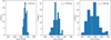 |
Fig. 3. Effect of the finite box size on the precision of our numerical simulations. Three-dimensional velocity dispersion ΔV3D in each of the 100 numerical realisations for the three configurations in Table 1 is shown as blue histograms. Vertical dashed line indicates the exact value of σturb from integration of the input turbulent power-spectrum (Eq. (14)). The increased numerical dispersions in those values as Linj increases as a consequence of the finite simulation box size. |
The emissivity of the galaxy cluster gas is taken as the square of a (isothermal, isometallic) gas density considered either as a spherical β-model (hereafter beta) or as a β-model along the line of sight and constant over the plane of the sky (hereafter Xbeta). The β parameter is held at a value of 2/3 while the core radius takes a value of {4, 21, 54, 107, 215, 429} kpc. The normalisation of the emissivity plays no objective role in this study, since no signal-to-noise consideration is made. Figure 4 shows one example of the line centroid and line width maps for a 200 kpc injection scale and the various beta emissivity models, free of any uncertainty other than numerical noise. In all numerical simulations there is no thermal broadening (σth = 0 km s−1 hereafter). In the following we present the comparisons with the Linj = 100 kpc simulation only. Validation of the other two runs is extensively presented in Appendix H for completeness.
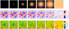 |
Fig. 4. Projection of a single realisation of a 3D velocity field (injection scale at 200 kpc) with several emissivity models (top row). All but the last column correspond to spherical β-models with core-radii of 4, 21, 54, 107, 215, and 429 kpc (from left to right). The rightmost column corresponds to a constant emissivity in the entire simulation box. The size of each panel is 520 kpc on a side. The middle row shows the centroid shift (C) and the bottom row shows the line width ( |

4.2. Centroid and line broadening
We first carry out the validation of Eqs. (8)–(11), which provide analytical representations of the sample average and variance of the line centroid shift and line broadening (more specifically, the square of the line width) measured in arbitrary apertures. We limit this validation exercise to circular apertures centred on a galaxy cluster and allow their sizes to vary.
These analytical expressions involve the calculation of the 3D function cϵ.𝒲: in Appendix B we provide the analytical formulas for both considered emissivity models and for circular apertures. Calculation of this function for spherical β-models demands slightly more computing time than for the Xbeta model.
Equation (11) requires integration over six scalar variables. Taking advantage of the isotropy of the velocity power spectrum and the 2D rotational invariance of this specific configuration, this can be reduced to five integration variables only (kx,  , ξ, ξ′, and one angle ϕ). This integral is evaluated by Monte-Carlo sampling distributed over 40 computing cores by means of the MCQUAD library3. The number of samplings is 2.106 and 2.105 for the Xbeta and beta emissivity models respectively, and we monitor and store the statistical uncertainties produced by the numerical sampler.
Figures 5 and 6 show the comparison between analytical calculations (plain lines) and numerical simulations (dots with error bars). They correspond to the Xbeta and beta emissivity models respectively, using the same 100 velocity boxes with Linj = 100 kpc. Each dot corresponds to a calculation using the 100 velocity realisations and a given core-radius size and a given aperture size. Error bars are derived from bootstrap resampling. Because we always used the same 100 simulations, the deviations from the expected trend appear correlated: this is striking for instance in the left-most panel showing ⟨C⟩. This behaviour is likely to disappear with a higher number of realisations.
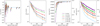 |
Fig. 5. Numerical validation of Eqs. (8)–(11). These are the expected value and sample variance of the line centroid shift C𝒲 (first and second panel) and the expected value and sample variance of the line width |

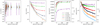 |
Fig. 6. Similar to Fig. 5 for a spherical β-model emissivity (beta). The numerical uncertainties are slightly larger (in the fourth panel, compared to Fig. 5) due to a lower accuracy in the numerical integration of Eq. (11). |
In any case these figures demonstrate a very good agreement between analytical calculations and simulations. The only exception is the case of very large core radii (rc = 429 kpc), for both emissivity models. This is a consequence of the simulation box being too small in the x-direction (4240 kpc along the line of sight). This causes a non-negligible sharp cutoff in the simulated β-emissivity profile, not accounted for by the analytical equations.
The sample variance of the centroid shift and the line width exhibit large variations with respect to the aperture radius. Emission line diagnostics in growing apertures for a selection of “look-alike” galaxy clusters has interesting potential to reveal the properties of the underlying turbulent power spectrum. This is illustrated in Fig. 7 where we vary the injection scale from 100 to 300 kpc for a given β-model (rc = 107 kpc). It is out of the scope of this paper to provide forecasts on the constraining power of this method, which must also include measurement uncertainties and limitations related to the availability of samples.
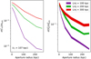 |
Fig. 7. Sample variance associated to line measurements. The centroid shift (left) and broadening (right) in apertures of growing sizes for clusters presenting identical emissivity models are shown for a spherical β-model with core radius of 107 kpc. These curves are predicted analytically by Eqs. (9) and (11). They have been normalised to the value of the 3D turbulent velocity dispersion σturb. The different shapes of the curves as the aperture radius grows can be used as a diagnostic to discriminate between various injection scales. |
4.3. Structure function
We restrict the numerical validation to that of Eqs. (12) and (13) for computational reasons. First, we consider an emissivity model of type Xbeta and a large enough analysis region compared to the typical separation and pixelisation of the line centroid map. The same 3 × 100 simulated boxes are projected and pixelised in square regions of size ℓ × ℓ, where ℓ = 4, 9, 17, 34, 69 kpc. Since the two-dimensional velocity field is stationary, it is fine to use  . This replacement is justified because in this configuration the surface brightness is constant over the analysis domain. In what follows the analysis domain is a circular aperture of diameter 520 kpc. Figure E.1 illustrates how pixelisation acts on a simulated centroid shift map: it is very close to a convolution or “smoothing”. Similar maps are created for all pixel sizes and core radii for all simulated boxes. The geometrical centres of the pixels are used to compute the structure function as the arithmetic mean of the squared centroid gradients at pre-defined separations s (within a range δs). The average of the structure functions and the standard deviations at each s provide the numerical indicators to be compared to Eqs. (12) and (13).
Analytical calculation of P2D is performed according to Eq. (C.3), by 2D convolution4 of the 3D velocity power spectrum P3D and the function Pρ at each frequency kx and eventual summing over those frequencies. The whole procedure is distributed over 40 processors working in parallel. Analytical expressions for Pρ are given in Appendix G (particularly Eq. (G.1)) for the emissivity models relevant to our validation procedure. The calculation of  is much more straightforward (see Eq. (C.4)).
A comparison between the analytical and numerical results is illustrated in Fig. 8 for a given turbulent power spectrum (injection scale at 100 kpc) and various values for the core radius and pixel size. The results from the 100 realisations are displayed as thin grey lines and their distribution at each s is likely not Gaussian. The analytical and numerical values for the sample variance are in very good agreement for all nine configurations, which is a very encouraging result given the various assumptions involved in both cases.
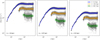 |
Fig. 8. Comparison of numerical and analytical structure functions and their sample variance for various cluster sizes (i.e. various core radii (rc) of the β-model) and various pixel sizes (ℓ). The data points and thick error bars show the sample mean and standard deviation of the 100 realisations (individually represented as thin grey lines) for each of the considered configurations. The coloured curves and shaded areas represent the analytical calculations following Eqs. (12) and (13). The emissivity model is Xbeta and the region of analysis is a circle of diameter 520 kpc (as displayed in Fig. E.1). The turbulent power spectrum is that of Table 1 with an injection scale of 100 kpc. |
A thorough assessment of the agreement between the analytical calculations and the numerical validation is summarised in Figs. 9 and 10. They show the relative difference (expressed in percent) between the analytical and the numerical computations for the expected value of the structure function and its variance, respectively. The injection scale is Linj = 100 kpc, as in Fig. 8. Three separations are illustrated: s = 20 kpc (close to the dissipation scale), s = 60 kpc (within the inertial range), and s = 300 kpc (past the inertial range).
 |
Fig. 9. Representation of the absolute relative difference between the numerical and analytical estimates of the sample mean of the structure function, ⟨SF⟩, at three distinct separations s. Each coloured square corresponds to one experiment based on the same 100 realisations of the velocity field with Linj = 100 kpc and various binning sizes (y-axis) and β-models core radii (x-axis). Small red crosses indicate locations where the binning size is larger than s. |
 |
Fig. 10. Similar to Fig. 9, but for the sample variance of the structure function, Var(SF). Positive values indicate higher predicted variance compared to that measured in the numerical validation procedure. Although some of these numbers are high at face value, it is important to recall the assumptions leading to the chosen analytical formula and the noise inherent in our set of numerical simulations (see text). |
Regarding the sample mean, the analytical model (Eq. (12)) performs well within 20% of the numerical experiment. Keeping in mind the limited number of realisations (100 samples), this result appears satisfactory. A degradation of the prediction accuracy arises as the binning size increases. This is attributed to numerical approximation in computing Pℓ and higher levels of sampling noise in the simulation (larger pixels imply fewer s-pairs). The slight decrease in accuracy at larger core radii was already pointed out in Sect. 4.2, as a result of the simulation box size.
As for the sample variance (Fig. 10), the relative differences between analytical and numerical results show somewhat higher values, as is expected for second order statistics. In general our formula tends to overpredict by a few tens of percent the observed variance of the structure function at small separations (s = 20 kpc) as a result of numerical uncertainties both in the simulations and the evaluation of integrals. At large separations (s = 300 kpc) and for the largest pixel size, the analytic formula underpredicts the variance by up to 80%. The analysis region 𝒜 indeed cannot be considered as infinitely large any longer, making simplification of Eq. (F.3) into Eq. (13) less accurate.
We finally relax the assumption of a constant emissivity and we show in Fig. 11 a comparison of the structure functions obtained for a spherical β-model density (beta emissivity model). The analytical formula Eq. (12) recovers the mean structure function, despite the spatial non-stationarity of the projected velocity field. We corrected for border effects using Eq. (D.3), the region analysis being a circle of diameter 520 kpc. As highlighted in Appendix E, we are not able to use the simple prescription for significantly large pixel binnings. Moreover we did not carry out the full evaluation of the sample variance using Eq. (F.3) for this figure. Instead, we computed the variance according to Eq. (13) assuming an effective core radius  . Such approximation of the complex emissivity field by an effective emissivity extracted at a radius of θeff = 80 kpc from the cluster centre makes the calculation more tractable. It shows a good agreement with results obtained from the Monte-Carlo simulations.
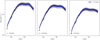 |
Fig. 11. Comparison of the simulated and calculated structure function in a similar way as Fig. 8, except the emissivity model is of type beta (spherical β-model gas density). This induces non-stationarity of the projected velocity field, noticeable by the drop at large s. The coloured curves represent the analytical calculation of the mean structure function following Eqs. (12) and (D.3). For simplicity, the variance remains calculated according to Eq. (13), that is assuming Xbeta emissivity with an effective core radius, |

5. Discussion
This work provides an extension of earlier studies, amongst others those of Inogamov & Sunyaev (2003), Churazov et al. (2012), Zhuravleva et al. (2012), and ZuHone et al. (2016). We extended the formalism presented in these papers by: (i) addressing the case of an arbitrary emissivity field; (ii) computing second order statistics beyond expected values (i.e. the sample variance), and (iii) identifying limiting cases in which these studies coincide.
5.1. Validity of hypotheses and range of applicability
Our study remains formal and relies on strong hypotheses such as uniform, ergodic, and isotropic turbulent velocity fields throughout the intra-cluster medium, whose physics are encapsulated in a universal Kolmogorov power spectrum, meaning that turbulence follows an identical physical description from cluster to cluster. The latter assumption is often implicitly made and mirrors an intent to concentrate all the unknown physics of turbulence in a single mathematical description. It is clear that this hypothesis may fail if widely distinct mechanisms produce turbulent motions: for instance large-scale matter accretion and central AGN feedback.
More specifically, our assumption of isotropic turbulent motions may break down in the stratified intra-cluster medium where buoyancy-restoring forces tend to suppress motions along the radial direction. Numerical simulations indicate a change in the morphology of turbulent fields in regions showing strong density gradients (e.g. Shi & Zhang 2019), even in cluster cores (Valdarnini 2019). According to these findings, one can therefore expect our model to become less representative as larger and larger cluster radii enter the emission line analysis, or in the presence of strong cool-core clusters. A study of anisotropic turbulence is out of the scope of this paper, but one could for instance undertake similar derivation steps as shown in the appendices, dropping the assumption  .
.
The existence of several drivers of turbulence acting at different scales may change the shape of the velocity power spectrum and more generally the statistical relations between Fourier coefficients of the velocity field. ZuHone et al. (2016) proposed to rewrite the resulting P3D as a sum of two Kolmogorov-like power spectra with different injection scales, based on the simulations and results of Yoo & Cho (2014). Such a prescription enters the framework presented in this paper, because our results are independent of the exact shape of P3D. However, it remains to be checked whether the decomposition of  proposed in Appendix F holds under such conditions, which most likely can be addressed through numerical simulations.
Our hypothesis also assumes full decoupling of the gas emissivity and the local behaviour of turbulent motions. This simplifying assumption may largely fail if gas motions are induced by the merging of an external galaxy group that shows high emissivity in its vicinity. An interesting perspective provided by the present calculations would be the coupling between P(k), the turbulent power spectrum, and ϵ, the emissivity; however, it is likely that calculations would become more complex and the gain over Monte-Carlo simulations would become less obvious. Moreover, density fluctuations, and hence emissivity fluctuations, are thought to be directly linked to the turbulent power spectrum based on theoretical grounds (Churazov et al. 2012). At first order though, the broad-scale emissivity of the galaxy cluster gas is the dominant component modulating the Doppler shift in the integrated line profiles and our approach remains a reasonable one in this regard.
Finally, our work deliberately neglects measurement uncertainties and instrumental noises. We address this assumption in a subsequent study (Paper II) by propagating the impact of measurement uncertainties on the line diagnostics, in particular the structure function. An interesting conclusion of this study is that sample variance effects dominate on large scales the error budget for observations based on next-generation X-ray instruments such as Athena/X-IFU, while statistics dominate at small scales.
5.2. Application: Forecasting line shift and width profiles
The formulas derived in Sect. 3 provide the sample mean and variance of both the line centroid shift and width in arbitrary apertures. As such, they can be used to predict measurements in concentric annuli centred on a galaxy cluster, that is, a radial profile. Formally, an annular aperture mask is defined as the difference between two concentric circular apertures. Thanks to the linear behaviour of the Fourier transform, the coefficient cϵ.𝒲 is also the difference between the two corresponding coefficients, both easily computed following Appendix B. Interestingly, the emissivity in each annulus can be considered as constant, ϵ(x, θ) = ϵ(x), if the gas density shows spherical symmetry and the annuli are thin enough. As already noted, this property drastically reduces the computing time needed to integrate the equations. An example of the profiles of centroid shift variance, line width average, and line width variance are displayed on Fig. 12 for a turbulent power spectrum with an injection scale of 100 kpc and σturb = 448 km s−1. No thermal broadening is included in this exercise. As expected, the centroid shift (whose average value is zero) shows larger variance in the central bins than the outskirts and the larger the core radius, the smaller the effect. The average broadening shows the reverse behaviour with smaller widths in the central parts and reaching a plateau (corresponding to σturb) in the outskirts. The line width variance shows diverse forms of behaviour but here again the general trend is a decrease towards the outskirts.
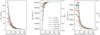 |
Fig. 12. Model predictions for radial profiles of line properties, which are those measurements in spectra collected in circularly concentric annuli of equal width (21 kpc). The figure shows the sample variance of the centroid shift (left panel), the sample average of the line broadening (middle panel), and the sample variance of the line broadening. The injection scale is Linj = 100 kpc, and the emissivity model is a spherical β = 2/3 model with core radii indicated in legend. Shaded rectangles indicate bin widths (horizontally) and numerical uncertainties (vertically). |
5.3. Forecasting the structure function from upcoming instrumentation
One particularly interesting perspective consists in inverting the formulas presented here to evaluate the power of future astronomical X-ray micro-calorimeters in constraining the nature of turbulent motions in galaxy clusters. By properly selecting the samples (typically, the number of objects and their core radii and distances) and the observing strategy (mapping, exposure times, etc.) one is able to focus the constraints for example on the slope of the power spectrum or the injection scale. This assumes that turbulence has identical characteristics throughout the sample considered, which hopefully is a reasonable guess. We postpone the complete exercise to later investigation. Rather we compute the expected structure functions for a simplified Coma-like galaxy cluster, following a setup similar to ZuHone et al. (2016) and using the associated uncertainties due to sample variance only (statistical errors are disregarded). We consider two instruments: (i) XRISM/Resolve with a resolution element of 1.5′ and a field of view of 3.4′ equivalent diameter, and (ii) Athena/X-IFU with a resolution element of 5″ and a field of view of 5′ equivalent diameter (Barret et al. 2018). We consider two observing strategies: either one single pointing towards the cluster centre, or the mapping of a ∼15′×15′ area with multiple pointings. We also consider the case of a 15″ pixelisation rebinned image for Athena/X-IFU, such that the signal-to-noise ratio of each spectrum is increased (e.g. Roncarelli et al. 2018, also Paper II). At the redshift of Coma, 1′ on sky corresponds roughly to a 27 kpc physical separation. We consider a turbulent power spectrum with σturb = 438 km s−1, α = −11/3, injection scale at 200 kpc, and dissipation scale at 20 kpc. Given the proximity of Coma and its apparent size, using the Xbeta emissivity model is amply justified, as already noted by Churazov et al. (2012) and ZuHone et al. (2016). Figure 13 shows the outcome of our model. For identical sky coverages, X-IFU provides smaller relative variance in comparison to Resolve, thanks to its better angular resolution. Even in one single pointing, X-IFU can provide a measurement of the structure function up to ∼100 kpc separation scales. The associated variance is larger though, due to a smaller number of pairs entering the structure function.
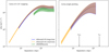 |
Fig. 13. Model predictions for structure functions and their associated sample variances under two instrumental setups: XRISM/Resolve (assuming 1.5′ resolution elements) and Athena/X-IFU (assuming 5″ and 15″ resolution elements for high and low signal-to-noise ratios respectively). Left panel: predictions for a ∼15′×15′ contiguous mapping of the Coma cluster while the right panel shows the result for a single X-IFU pointing. A single Resolve pointing (3′ on a side) would be too small for a useful derivation of the structure function. The text gives further details on the input turbulent power spectrum and gas density model. |
This example provides the basis for further research, in view of optimising an observational strategy for a given instrumental setup. Our formalism involves Fourier transforms of window functions (denoted 𝒜 and 𝒲) and therefore accounts for arbitrary instrumental shapes and pointing strategies, by taking advantage of standard properties of the Fourier transform. For instance, a window function made of multiple non-overlapping pointings can be considered as a sum of identical, translated window functions; linearity then makes the computation of its Fourier transform straightforward.
6. Conclusions
In this paper we have derived analytical expressions for the sample mean and variance of three indicators of turbulence in X-ray emitting, optically-thin plasmas under the hypothesis of homogeneous and isotropic Kolmogorov turbulence. These are the line centroid shift C, the line broadening S, and the structure function SF.
-
We obtained exact expressions for the mean and variance of C and S obtained from single line-of-sight measurements through arbitrary gas emissivity. These expressions are Eqs. (4)–(7). We numerically validated the results with Monte-Carlo simulations of turbulent velocities with Gaussian or constant amplitudes.
-
We generalised these expressions for measurements in apertures of arbitrary shapes and sizes and for arbitrary three-dimensional emissivity fields, demonstrated in Eqs. (8)–(11). In Appendix B we provide useful formulas for the common β-model and for circular apertures. We numerically validated the formulas using Monte-Carlo simulations of 3D velocity fields in a range of emissivity and power-spectrum configurations.
-
We derived an expression for the mean structure function under the assumption of negligible border effects (Eq. (12)). Notably, this formula does not assume constant (“flat”) emissivity in the plane-of-sky direction. It involves a specific definition for the two-dimensional power spectrum of the projected velocity field, introduced in Appendix C. In Appendix G we provide useful formulas for the common β-model and for circular domains of analysis.
-
In Appendix D we provide a correction formula for border effects (Eq. (D.3)) valid for non-binned maps of the projected velocity and for domains of arbitrary shapes. We explicitly computed the case of a circular field of view.
-
In Appendix E we provide a simple prescription to account for binning (or pixelisation) on the mean structure function. It is valid as long as pixels are smaller than the typical scale of flux variations and much smaller than the domain of analysis.
-
We derived a fairly generic expression for the sample variance of SF under the assumption of negligible border effects and for arbitrary emissivity fields (Eq. (F.3)). This equation takes a tractable form in case of flat emissivity and very large domain of analysis (Eq. (13)).
-
We numerically validated our results for the sample mean and variance of SF in the case of “flat” emissivity fields (β-models with a range of core radii) and various binnings.
-
We numerically validated our results for the sample mean of SF in the case of non-flat emissivity fields (spherical β-models with a range of core radii) and negligible binning.
We discussed our results and presented forecasts for observations of the core of the Coma cluster with the integral field units X-ray calorimeters5 planned to embark onboard XRISM (Resolve) and Athena (X-IFU).
There is some flexibility in choosing the definition of distance, either considering geometrical centres of each region, flux-weighted barycentres or other factors.
Available in package SciKit-Monaco, https://pypi.org/project/scikit-monaco
Making use of the FFT convolution implemented in the signal.convolve function of Numpy/Scipy.
The case in which kx = 0 is recovered using limx → 0xnKn(x) = π2n − 1/[sin(nπ)Γ(1−n)] (Spiegel 2003).
This is because 
Acknowledgments
The authors thank the referee for useful comments that helped to improve the quality and perspectives of this work. The authors thank D. Barret for fruitful discussions that led to the improvement of this manuscript. NC thanks A. Marin-Laflèche for help in the selection of an FFT algorithm suited to this research, A. Proag for useful discussions on geometrical calculations, and L. Le Briquer for commenting on a preliminary version of this manuscript. This research made use of Astropy, a community-developed core Python package for Astronomy (Astropy Collaboration 2013; Price-Whelan et al. 2018). This research made use of Matplotlib (Hunter 2007).
References
- Anorve-Zeferino, G. A. 2019, MNRAS, 483, 704 [NASA ADS] [CrossRef] [Google Scholar]
- Armstrong, M. 1998, Basic Linear Geostatistics (Springer Science & Business Media) [CrossRef] [Google Scholar]
- Astropy Collaboration (Robitaille, T. P., et al.) 2013, A&A, 558, A33 [NASA ADS] [CrossRef] [EDP Sciences] [Google Scholar]
- Barret, D., Lam Trong, T., den Herder, J. W., et al. 2016, in Space Telescopes and Instrumentation 2016: Ultraviolet to Gamma Ray, SPIE Conf. Ser., 9905, 99052F [Google Scholar]
- Barret, D., Lam Trong, T., den Herder, J. W., et al. 2018, in Space Telescopes and Instrumentation 2018: Ultraviolet to Gamma Ray, SPIE Conf. Ser., 10699, 106991G [Google Scholar]
- Cavaliere, A., & Fusco-Femiano, R. 1978, A&A, 70, 677 [NASA ADS] [Google Scholar]
- Cayón, L. 2010, MNRAS, 405, 1084 [NASA ADS] [Google Scholar]
- Churazov, E., Vikhlinin, A., Zhuravleva, I., et al. 2012, MNRAS, 421, 1123 [NASA ADS] [CrossRef] [Google Scholar]
- Corstanje, R., Grunwald, S., & Lark, R. 2008, Geoderma, 143, 123 [Google Scholar]
- Cressie, N. 1985, J. Int. Assoc. Math. Geol., 17, 563 [CrossRef] [Google Scholar]
- Cucchetti, E., Clerc, N., Pointecouteau, E., Peille, P., & Pajot, F. 2019, A&A, 629, A144 (Paper II) [NASA ADS] [CrossRef] [EDP Sciences] [Google Scholar]
- Esquivel, A., Lazarian, A., Horibe, S., et al. 2007, MNRAS, 381, 1733 [NASA ADS] [CrossRef] [EDP Sciences] [Google Scholar]
- Gaspari, M., Churazov, E., Nagai, D., Lau, E. T., & Zhuravleva, I. 2014, A&A, 569, A67 [Google Scholar]
- Gaspari, M., McDonald, M., Hamer, S. L., et al. 2018, ApJ, 854, 167 [NASA ADS] [CrossRef] [Google Scholar]
- Haslett, J. 1997, J. R. Stat. Soc. Ser. D (The Statistician), 46, 475 [CrossRef] [Google Scholar]
- Hunter, J. D. 2007, Comput. Sci. Eng., 9, 90 [NASA ADS] [CrossRef] [Google Scholar]
- Inogamov, N. A., & Sunyaev, R. A. 2003, Astron. Lett., 29, 791 [NASA ADS] [CrossRef] [Google Scholar]
- Ishisaki, Y., Ezoe, Y., Yamada, S., et al. 2018, J. Low Temp. Phys., 193, 991 [Google Scholar]
- Kolmogorov, A. 1941, Akademiia Nauk SSSR Doklady, 30, 301 [Google Scholar]
- Li, N., & Laizet, S. 2010, Proceedings of Cray User Group 2010 Conference, Edinburgh [Google Scholar]
- Lis, D. C., Keene, J., Li, Y., Phillips, T. G., & Pety, J. 1998, ApJ, 504, 889 [NASA ADS] [CrossRef] [Google Scholar]
- Martínez, V., Arnalte-Mur, P., & Stoyan, D. 2010, A&A, 513, A22 [NASA ADS] [CrossRef] [EDP Sciences] [Google Scholar]
- Matheron, G. 1965, Les Variables régionalisées et leur estimation: une application de la théorie des fonctions aléatoires aux sciences de la nature (Masson et Cie) [Google Scholar]
- Matheron, G. 1973, Adv. Appl. Prob., 5, 439 [CrossRef] [Google Scholar]
- Miniati, F., & Beresnyak, A. 2015, Nature, 523, 59 [Google Scholar]
- Price-Whelan, A. M., Sipőcz, B. M., Günther, H. M., et al. 2018, AJ, 156, 123 [NASA ADS] [CrossRef] [Google Scholar]
- Roelens, M., Eyer, L., Mowlavi, N., et al. 2017, MNRAS, 472, 3230 [NASA ADS] [CrossRef] [Google Scholar]
- Roncarelli, M., Gaspari, M., Ettori, S., et al. 2018, A&A, 618, A39 [NASA ADS] [CrossRef] [EDP Sciences] [Google Scholar]
- Ryu, D., Kang, H., Cho, J., & Das, S. 2008, Science, 320, 909 [NASA ADS] [CrossRef] [PubMed] [Google Scholar]
- Shi, X., & Zhang, C. 2019, MNRAS, 487, 1072 [NASA ADS] [CrossRef] [Google Scholar]
- Spiegel, M. 2003, Manual de fórmulas y tablas matemáticas: 2400 fórmulas y 60 tablas, Serie de compendios Schaum (McGraw-Hill/Interamericana) [Google Scholar]
- Valdarnini, R. 2019, ApJ, 874, 42 [Google Scholar]
- Vazza, F., Angelinelli, M., Jones, T. W., et al. 2018, MNRAS, 481, L120 [NASA ADS] [CrossRef] [Google Scholar]
- Yoo, H., & Cho, J. 2014, ApJ, 780, 99 [Google Scholar]
- Zhuravleva, I., Churazov, E., Kravtsov, A., & Sunyaev, R. 2012, MNRAS, 422, 2712 [NASA ADS] [CrossRef] [Google Scholar]
- Zhuravleva, I., Churazov, E., Schekochihin, A. A., et al. 2014, Nature, 515, 85 [Google Scholar]
- ZuHone, J. A., Markevitch, M., & Zhuravleva, I. 2016, ApJ, 817, 110 [NASA ADS] [CrossRef] [MathSciNet] [Google Scholar]
Appendix A: Calculations in the one-dimensional case
This appendix details the calculation leading to the results presented in Sect. 2, namely the expected values for the centroid shift C and line broadening S2 and their variances, in the case of measurements along a single line of sight (Eq. (4)–(7)). These calculations are generalised in Sect. 3 for two-dimensional diagnostics of the velocity field.
A.1. Statistics of the centroid
The finding ⟨C⟩=0 is a direct consequence of random uncorrelated phases. We calculate Var(C) = ⟨C2⟩ by noting that
 (A.1)
(A.1)
From Eq. (3), the term within brackets reads
It is then easily shown that
The term within modulus is  , namely the kth Fourier coefficient of ϵ. This identification leads to the expression shown in Eq. (5).
A.2. Statistics of the dispersion
The variations of S2 are due to the second term of Eq. (2), therefore we will focus now on studying the statistics of the double integral ∬G.
A.2.1. Average of ∬G
First we write
![Mathematical equation: $$ \begin{aligned} A \equiv \left\langle \int \int G \right\rangle = \int \int \langle G \rangle = \int \int \epsilon (x) \epsilon (x^{\prime }) \left\langle \left[v(x)-v(x^{\prime })\right]^2\right\rangle \end{aligned} $$](/articles/aa/full_html/2019/09/aa35676-19/aa35676-19-eq77.gif)
and
Therefore, using Eq. (3)
![Mathematical equation: $$ \begin{aligned} \left\langle \left[ v(x)-v(x^{\prime }) \right]^2 \right\rangle&= \sum _k P(k) \left| e^{i k\omega x} - e^{i k\omega x^{\prime }} \right|^2\\ &= 2 \sum _k P(k) \left[ 1- \cos (k \omega (x^{\prime }-x)) \right] . \end{aligned} $$](/articles/aa/full_html/2019/09/aa35676-19/aa35676-19-eq79.gif)
This leads to
![Mathematical equation: $$ \begin{aligned} A =&2 \sum _k P(k) \int \int \mathrm{d} x \mathrm{d} x^{\prime } \epsilon (x) \epsilon (x^{\prime })\\&\times \left[1- \cos (k \omega x^{\prime }) \cos (k \omega x) - \sin (k \omega x^{\prime }) \sin (k \omega x) \right] . \end{aligned} $$](/articles/aa/full_html/2019/09/aa35676-19/aa35676-19-eq80.gif)
This expression again can be rewritten using the power spectrum of the emissivity
![Mathematical equation: $$ \begin{aligned} A = 2 \sum _k P(k) \left[ F^2 - P_{\epsilon }(k) \right]. \end{aligned} $$](/articles/aa/full_html/2019/09/aa35676-19/aa35676-19-eq81.gif) (A.2)
(A.2)
The average of the measured line width then reads
![Mathematical equation: $$ \begin{aligned} \left\langle S^2 \right\rangle = \frac{1}{F} \int \epsilon (x) \sigma _{\rm th}^2(x) \mathrm{d} x + \sum _k P(k) \left[ 1 - \frac{P_{\epsilon }(k)}{F^2} \right], \end{aligned} $$](/articles/aa/full_html/2019/09/aa35676-19/aa35676-19-eq82.gif)
which we write under the simple form
where a horizontal bar denotes averaging of the thermal component along the line of sight.
A.2.2. Variance of ∬G
We define B such that Var(S2)=F−4(B2 − A2)/4. We note that
![Mathematical equation: $$ \begin{aligned} \left\langle \left( \int \int G \right)^2 \right\rangle&= B^2\nonumber \\&= \int \epsilon (x) \epsilon (y) \epsilon (z) \epsilon (t)\nonumber \\ &\quad \left\langle \left[ v(x)-v(y) \right]^2 \left[ v(z)-v(t) \right]^2 \right\rangle \mathrm{d} x \mathrm{d} y \mathrm{d} z \mathrm{d} t. \end{aligned} $$](/articles/aa/full_html/2019/09/aa35676-19/aa35676-19-eq84.gif) (A.3)
(A.3)
The term within brackets reads
![Mathematical equation: $$ \begin{aligned} \left\langle [.]^2 \times [.]^2 \right\rangle =&\sum _{j,k,l,m} \langle V_j V_ k V_l V_m \rangle \times \left( e^{i k \omega x} - e^{i k \omega y}\right) \left( e^{i j \omega x} - e^{i j \omega y} \right)\nonumber \\&\times \left( e^{i l \omega z} - e^{i l \omega t} \right) \left( e^{i m \omega z} - e^{i m \omega t} \right) . \end{aligned} $$](/articles/aa/full_html/2019/09/aa35676-19/aa35676-19-eq85.gif) (A.4)
(A.4)
Since phases are two-by-two independent, we assume the simplest possible expression for the four-term product of Fourier coefficients Vk, namely:
All cases are mutually exclusive. Noting that conditions B and C lead to identical expressions under transformation l ↔ m, and similarly for D and E, we can rewrite the sum, and hence the triple integral, with a sum of four terms:

First term: If (k = −j) and (l = −m) the bracket is written
After some algebra, the integration over x, y, z, and t provides
![Mathematical equation: $$ \begin{aligned} b_A&= 4 \sum _{j \ne \pm k} P(k) P(j) \left[ F^4 - F^2 P_{\epsilon }(k) - F^2 P_{\epsilon }(j) + P_{\epsilon }(k) P_{\epsilon }(j) \right]\nonumber \\&= 4 \sum _{j \ne \pm k} P(k) P(j) \left[ F^2 - P_{\epsilon }(k) \right] \left[ F^2 - P_{\epsilon }(j) \right], \end{aligned} $$](/articles/aa/full_html/2019/09/aa35676-19/aa35676-19-eq89.gif) (A.5)
(A.5)
where we have used the same trigonometric decomposition as in the derivation of Eq. (A.2).
Second term: The symmetries in the expression lead to
introducing the complex function

Developing the product fkfj we can rewrite the term under the modulus as
Third term: The term within brackets is rewritten as
which, using similar calculations as for bA, leads to
![Mathematical equation: $$ \begin{aligned} b_D = 4 \sum _k \left\langle |V_k|^4 \right\rangle \left[F^2 - P_{\epsilon }(k) \right]^2. \end{aligned} $$](/articles/aa/full_html/2019/09/aa35676-19/aa35676-19-eq94.gif)
Fourth term: In a similar way to the computation of bF above, we find
Therefore, combining previous expressions we obtain
![Mathematical equation: $$ \begin{aligned} \mathrm{Var} (S^2) =&2 \sum _{j \ne \pm k} P(k)P(j) \left| \frac{\widetilde{\epsilon }(j+k)}{F}-\frac{\widetilde{\epsilon }(j) \widetilde{\epsilon }(k)}{F^2} \right|^2 \\&+ \sum _k \left\langle |V_k|^4 \right\rangle \left| \frac{\widetilde{\epsilon }(2k)}{F} - \frac{\widetilde{\epsilon }(k)^2}{F^2} \right|^2 \\& + 2 \sum _k \left( \langle |V_k|^4 \rangle - P(k)^2 \right) \left[ 1- \frac{P_{\epsilon }(k)}{F^2} \right]^2, \end{aligned} $$](/articles/aa/full_html/2019/09/aa35676-19/aa35676-19-eq96.gif)
which is rearranged to provide Eq. (7).
Appendix B: Fourier transform of the emissivity field ϵ ( β-model)
We provide here calculations of cϵ.𝒲, the 3D power spectrum of the emissivity ϵ(x, y, z) in the case of a β-model, seen through a sky aperture 𝒲(y, z). This is particularly useful for deriving the line centroid and broadening statistics. We assume that  where ne is the gas density and effectively follows a β-model profile, as in an isothermal, isometallic intra-cluster medium.
B.1. Spherical model
For a spherical β-model density with core radius rc centred on θ = 0, the emissivity is expressed as
The flux integrated along the line of sight is written
 (B.1)
(B.1)
The value of cϵ.𝒲 is defined as
This Fourier transform is calculated first along the x-axis,
![Mathematical equation: $$ \begin{aligned}&\int _{- \infty }^{+\infty } \left( 1+ \frac{x^2+\theta ^2}{r_c^2} \right)^{-3\beta } e^{-i \omega k_x x} \mathrm{d} x\nonumber \\&\qquad \qquad \quad = 2 r_c^{6 \beta } (\omega |k_x|)^{6 \beta -1} \int _0^{+ \infty } \frac{\cos (t) \mathrm{d} t}{\left[ (\omega k_x)^2 (\theta ^2 + r_c^2) + t^2\right]^{3 \beta }} \nonumber \\&\qquad \qquad \quad = \frac{2^{3/2-3\beta } \sqrt{\pi }}{\Gamma (3 \beta )} r_c^{6 \beta } \left( \frac{\sqrt{\theta ^2 + r_c^2}}{\omega |k_x|} \right)^{1/2-3 \beta } K_{3\beta -1/2}\left(\omega |k_x| \sqrt{\theta ^2+r_c^2}\right) , \end{aligned} $$](/articles/aa/full_html/2019/09/aa35676-19/aa35676-19-eq101.gif) (B.2)
(B.2)
where Kn is the modified Bessel function of the second kind6. In the special case of β = 2/3, this formula is equivalent7 to Eq. (23) in ZuHone et al. (2016), namely  , with
  .
.
Introducing ℱn(x)=xnKn(x), the integration over the plane-of-sky coordinates θ provides
 (B.3)
(B.3)
The unknown normalisation factor ϵ(0) is unimportant in this paper, since the Fourier transform always appears divided by the aperture flux F𝒲 defined by
An usual practical case is for a circular aperture 𝒲 of radius Rap centred on θ = 0. For this particular case,
![Mathematical equation: $$ \begin{aligned} \frac{c_{\epsilon .\mathcal{W} }}{F_{\mathcal{W} }}(k_x, \boldsymbol{\xi }) =&\frac{2^{5/2-3\beta } (3\beta -3/2)}{\Gamma (3\beta -1/2)} \left( 1- \left[ 1+ \frac{R_{\rm ap}^2}{r_c^2} \right]^{3/2-3\beta } \right)^{-1} \\ &\times \mathcal{I} _{(R_{\rm ap}/r_c); (3\beta -1/2)}\left(\omega |k_x|r_c, \omega \xi r_c\right) , \end{aligned} $$](/articles/aa/full_html/2019/09/aa35676-19/aa35676-19-eq106.gif)
which uses the special integral defined below and represented in Fig. B.1 for n = 3/2 (β = 2/3):
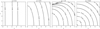 |
Fig. B.1. Numerical calculations of ℐp; n(u, v) for various values of p and n = 3/2. Logarithmically-spaced contours (identical in all panels) indicate the value of the function. This function is involved in the calculation of the Fourier transform of a spherical β-model (n = 3β − 1/2) observed through a concentric circular aperture of radius p times the core radius. |
B.2. Plane-constant model
The integral B.3 can be simplified if the core radius rc is much larger than the typical size of the window function 𝒲. In such a case, it is equivalent to consider an emissivity that is independent of the line-of-sight direction θ, that is, ϵ(x, y, z)=ϵ(x). An effective impact parameter θeff is introduced so that
The calculations above then become
 (B.4)
(B.4)
where we introduced  and 𝒮𝒲 = ∫𝒲 is the area of the aperture on sky and
  its (2D) Fourier transform.
An usual practical case is for a circular aperture 𝒲 of radius Rap and an emissivity ϵ(x) in the form of a β = 2/3-model independent of the line of sight. For this particular case,
with J1 the Bessel function of the first kind and order 1.
Appendix C: Two-dimensional power spectrum for generic emissivity field
For a pencil-beam aperture 𝒲(θ′) = δ(θ − θ′), the expression for the centroid shift is written
Since χθ(x)=ρ(x, θ), we obtain
 (C.1)
(C.1)
where the tilde indicates a one-dimensional Fourier transform along direction x. Indeed,
 (C.2)
(C.2)
with  the (3D) Fourier transform of ρ. The last equality derives from the definition of the inverse 3D Fourier transform.
We note that ρ(x, y, z)=ϵ/F is defined in a domain of space 𝒜 (area 𝒮𝒜) where the flux F(y, z) of the source is non-zero (which in practice is a bounded region). If the source is infinitely extended (as in the formal case of a β-model), the boundary is imposed by the domain of analysis 𝒜, for example the instrument field of view. We therefore consider that ρ is defined over the entire 3D space by filling regions outside of the bounded domain with zeros, which ensures the existence of  . The 2D Fourier transform
  of C(θ) is used to define
The weighting by the total area ensures that the total “energy” does not diverge as 𝒜 becomes large. We provide later the expression for the limiting case of an infinitely extended analysis domain.
Equation (C.2) shows that at any given kx,  is the 2D inverse Fourier transform of
  and then
Therefore,
which leads to
Averaging over all possible realisations provides
which is equivalent to
 (C.3)
(C.3)
We note that P2D is in general non-isotropic, as the emissivity and the shape of the analysis domain are arbitrary. However, in the particular case where the normalised line-of-sight emissivity is independent of the line of sight, and thus following our previous notations χθ(x)≡ϵ(x)/F, we find that
with
This leads to the expression
with ⊗ representing the discrete convolution product. The power spectrum  is defined such as it matches P2D for an extremely large domain of analysis. Indeed, P𝒜 then becomes a very peaked function around ξ = 0 and we obtain (see also Zhuravleva et al. 2012)
 (C.4)
(C.4)
Appendix D: Structure function for generic emissivity field
D.1. Formal derivation neglecting border effects
For convenience, we introduce the 𝒲-normalised emissivity:  . By extension, we define χθ(x)=ϵ(x, θ)/F(θ)=ρ(x, θ). We recall that ρ = 0 outside of the domain of analysis by construction, this is equivalent to imposing that the centroid shift vanishes outside of this region. Using the decomposition of the velocity field in Fourier series and the definition of the velocity power spectrum, one obtains
which for the most common “pencil-beam” window function, 𝒲θ = δ(θ0 − θ), reduces to
 (D.1)
(D.1)
with
![Mathematical equation: $$ \begin{aligned} C_{\boldsymbol{\theta }_0,\boldsymbol{r}}(\boldsymbol{\underline{k}}) = \int \mathrm{d} x e^{ik_x \omega x} \left[ \chi ^{\boldsymbol{\theta }_0+ \boldsymbol{r}}(x) e^{i \omega \boldsymbol{\xi } \cdot \boldsymbol{r}} - \chi ^{\boldsymbol{\theta }_0}(x) \right] . \end{aligned} $$](/articles/aa/full_html/2019/09/aa35676-19/aa35676-19-eq135.gif)
The expected value for the structure function therefore is written
with
Following notations in the previous appendix, we can rewrite  into
into

We then obtain
![Mathematical equation: $$ \begin{aligned} |C_{\boldsymbol{\theta }, \boldsymbol{r}}(\boldsymbol{\underline{k}})|^2 = |\widetilde{\chi ^{\boldsymbol{\theta }}}(k_x)|^2 + |\widetilde{\chi ^{\boldsymbol{\theta } + \boldsymbol{r}}}(k_x)|^2 - 2 \times \mathrm{Re} \left[ e^{i\omega \boldsymbol{\xi } \cdot \boldsymbol{r}} \widetilde{\chi ^{\boldsymbol{\theta }}}^{*}(k_x) \widetilde{\chi ^{\boldsymbol{\theta }+ \boldsymbol{r}}}(k_x) \right] . \end{aligned} $$](/articles/aa/full_html/2019/09/aa35676-19/aa35676-19-eq140.gif)
In a first approximation, let us perform a summation over all pairs, including those fully comprised within the domain of analysis 𝒜 (“inner” pairs on Fig. D.1) and those with only one end in 𝒜 (“Ext” pairs). By construction  for θ outside of 𝒜. This approximation is equivalent to neglecting border effects and correction terms are discussed in the following subsection.
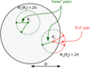 |
Fig. D.1. Sketch illustrating the counting of pairs within a circular domain of analysis of radius R represented by the large black circle. Within this domain, the centroid shift C(θ) takes values determined by the stochastic turbulent field, while we set C = 0 outside. Counting inner pairs (shown with green and red sticks) separated by a distance s is performed by computing the range of accessible angles ϕs(θ) for a given position in the domain, then dividing by two. External pairs have only one end within the domain of analysis and the range of accessible angles is 2π − ϕs at a given position. |
Using the relation between  and
and  identified previously, we obtain

Using Eq. (C.2) and some algebra leads to

Summing the term under the Re function over all pairs (without double counting), we write
![Mathematical equation: $$ \begin{aligned} \int _{p} \left[ e^{i\omega \boldsymbol{\xi } \cdot \boldsymbol{r}} \widetilde{\chi ^{\boldsymbol{\theta }}}^{*}(k_x) \widetilde{\chi ^{\boldsymbol{\theta }+ \boldsymbol{r}}}(k_x) \right]&= \frac{1}{2} \int _{\boldsymbol{\theta }} \int _{|\boldsymbol{r}|=s} \left[ e^{i\omega \boldsymbol{\xi } \cdot \boldsymbol{r}} \widetilde{\chi ^{\boldsymbol{\theta }}}^{*}(k_x) \widetilde{\chi ^{\boldsymbol{\theta }+ \boldsymbol{r}}}(k_x) \right] \\&= \frac{1}{2} \left(\frac{\omega }{2\pi }\right)^2 \int \mathrm{d} \boldsymbol{\xi }^{\prime } P_{\rho }(k_x,\boldsymbol{\xi }^{\prime }) \int _{0}^{2\pi } e^{i \omega |\boldsymbol{\xi } + \boldsymbol{\xi }^{\prime }| s \cos \phi } \mathrm{d} \phi \\&= \pi \left(\frac{\omega }{2\pi }\right)^2 \int \mathrm{d} \boldsymbol{\xi }^{\prime } P_{\rho }(k_x,\boldsymbol{\xi }^{\prime }) J_0(\omega |\boldsymbol{\xi } + \boldsymbol{\xi }^{\prime }| s). \end{aligned} $$](/articles/aa/full_html/2019/09/aa35676-19/aa35676-19-eq146.gif)
We finally obtain
![Mathematical equation: $$ \begin{aligned} I_{s}(\boldsymbol{\underline{k}}) = 2 \pi \left(\frac{\omega }{2\pi }\right)^2 \int \mathrm{d}\boldsymbol{\xi }^{\prime } P_{\rho }(k_x,\boldsymbol{\xi }^{\prime }) \left[ 1 - J_0\left(\left| \boldsymbol{\xi } + \boldsymbol{\xi }^{\prime } \right| \omega s \right) \right] . \end{aligned} $$](/articles/aa/full_html/2019/09/aa35676-19/aa35676-19-eq147.gif) (D.2)
(D.2)
Dividing by the total number of pairs  provides the general expression for the expected value of the structure function (see Eq. (12)). These calculations assume that integration over all pairs (θ, r) is continuous. Appendix E describes the effect of pixelised and filtered data.
D.2. Finite-sized effects (circular domain of analysis)
Previous calculations neglect border effects in the integration over pairs of points. We have set ρ = 0 outside of the domain of analysis, which implies C = 0. Consequently a number of extra pairs are erroneously included in this derivation, translating into extra terms ⟨|C(θ + r)−C(θ)|2⟩=⟨|C(θ)|2⟩ in the numerator Is and the number of pairs entering the denominator Np(s) needs to be corrected (see Fig. D.1).
The integrals shown previously run over all pairs separated by s with at least one extremity within the field of view. There are  such pairs and
  pairs with only one end within the field of view. Naturally we denote
  the pairs fully comprised within the domain analysis. A given point θ in the analysis domain belongs to ϕs(θ)∈[0, 2π] pairs in the field of view. Let us first compute the exact number of pairs, assuming an infinitely fine tessellation,
We write
denoting by  the value of the structure function corrected from finite-sized effects. We obtain
As demonstrated in Sect. 2,
Reassembling terms, we obtain the corrected mean structure function (sfcorr):
 (D.3)
(D.3)
The correction term depends both on the number of extra pairs and on their separation s relative to the size of velocity fluctuations.
We have
Estimating ϕ is easy under the assumption of a circular analysis region of radius R. We find the following expressions, graphically represented in Fig. D.2, left:
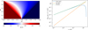 |
Fig. D.2. Counting pairs in the circular analysis region. Left: two-dimensional representation of the function ϕs(θ) for various values of the separation s and the position θ in a circular field of view of radius R. Right: scaling of Np(s), the number of pairs of points separated by a distance s within a circular field of view of radius R. “Inner” concerns those pairs integrally contained within the circular domain, while “Ext” concerns those pairs with only one end within the domain. “All” is the sum of the two numbers. The curves actually show δ(sNp(s))/δs, which is the differential number of pairs per interval of s expressed in units of the radius R. Here ℓ ≪ R is the side length of an elementary pixel, so that the total number of pixels in the circle is πR2/ℓ2. |
We therefore rewrite  and
and  with
with

and
![Mathematical equation: $$ \begin{aligned} G(x) = \left\{ \begin{array}{cl} 4 \pi \int _{x-1}^{x} \left[ \pi - \gamma (u;x) \right] u \mathrm{d} u&\mathrm if \ x>1 \\ 2 \pi ^2 (1-x)^2 + 4 \pi \int _{1-x}^x \left[ \pi - \gamma (u;x) \right] u \mathrm{d} u&\mathrm if \ 0.5 < x < 1 \\ \end{array}\right. \end{aligned} $$](/articles/aa/full_html/2019/09/aa35676-19/aa35676-19-eq163.gif)
having introduced  .
.
The expressions for the number of pairs as a function of the separation distance are represented in Fig. D.2. As expected, the number of extra pairs is negligible for small pair separations. It equals the number of regular (“inner”) pairs for s ≃ 0.5R and becomes dominant past this value.
Finally, we note that for the flat emissivity field (ρ(x, θ)=ϵ(x)/F) we have  and then
 (D.4)
(D.4)
Since in this case the projected velocity field is stationary and isotropic, it may be easier and more exact to compute the mean structure function using  in Eq. (12), instead of involving P2D and applying this correction formula. This property is used to check the validity of the correction formula in Eq. (D.4). Figure D.3 shows the result of our calculation for a flat emissivity field with core radius rc = 400 kpc and a turbulent power spectrum with injection scale Linj = 10Ldiss = 200 kpc. The domain of analysis is circular with a radius of R = 70, 120, or 500 kpc. The result for an unbounded domain is also shown. For small analysis domains (R = 70 kpc) the uncorrected formula induces discrepancies at small separations, due to the high-pass behaviour of the mask 𝒜. As the field of view increases (R = 500 kpc), border effects become negligible and all structure functions match the exact one. Finally, as
  approaches zero for a separation length of size s = 2R, the correction formula becomes numerically unstable at large separation lengths.
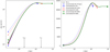 |
Fig. D.3. Impact of finite-sized corrections on the mean structure functions computed according to our model. The domain of analysis is a circle of radius R. Both panels show the same data, in logarithmic or linear scales. The emissivity model is of type Xbeta with a core radius rc = 400 kpc. The turbulent power spectrum has injection and dissipation scales Linj and Ldiss respectively. The thick dashed line is barely visible and shows the exact result obtained assuming an infinitely extended analysis domain. Points at large separations s are subject to slight numerical instabilities. |
Appendix E: Structure function from pixelised and/or filtered data
Previous derivations assume that the centroid shift can be measured along every line of sight. In general, real datasets are convolved by an instrumental point spread function and a pixel design effectively groups lines of sight within a single spectral line measurement. Both processes are formally close to each other, since pixelisation along a regular grid can be reformulated as a top-hat filtering followed by the selection of points at the centre of each pixel (Fig. E.1).
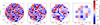 |
Fig. E.1. Effect of a larger pixelisation when computing the structure function. Pixel size ranges from ℓ = 4, 17, 34, 69 kpc (from left to right). All four panels represent the same projected velocity field (injection scale at 100 kpc) in a galaxy cluster represented by a Xbeta model of core radius 21 kpc. In general, larger pixels reduce the power in the two-dimensional velocity fluctuations and roughly act like a smoothing convolution filter on the high-resolution centroid map. |
We define a new map D(θ) as
 (E.1)
(E.1)
where represents the usual convolution product, and F(θ) and C(θ) are respectively the flux and centroid maps as defined in Sect. 3.1. The filter ℱℓ may represent the instrumental point spread function, or the pixel window function (previously denoted 𝒲) or a combination of the two; we assume its characteristic scale is ℓ (e.g. instrument full width at half maximum, pixel size, etc.) and it is normalised to 1 by integrating over all values of θ. It is clear that D(θ) is the value of the centroid shift measured after the filtering process, resulting from a flux-weighted average of individual centroid shifts.
This formula reduces to D(θ)≃C(θ) for components of C varying on scales much larger than ℓ (equivalently, for very sharp filters). For components of C oscillating on tiny scales (much smaller than the filter size), we find D ≃ 0: as expected the pixelisation or filtering process suppresses information on small scales.
A useful derivation can be carried out in the case of a smooth flux map, varying on scales much larger than the filter size ℓ. Then F can be considered constant in the convolution products and one obtains D ≃ ℱℓ * C. All previous calculations now must incorporate this convolution product. For instance, the following replacement takes place:
The calculation steps are similar to the previous case, thanks to permutations of the integrals over μ and other integrals. This calculation leads to the expected value of the structure function at each s:
![Mathematical equation: $$ \begin{aligned} \mathrm{sf} (s)&= 2 \sum _{\boldsymbol{\underline{k}}} P_{\rm 3D}(k) \int \mathrm{d} \boldsymbol{\xi }^{\prime } P_{\rho }(k_x,\boldsymbol{\xi }^{\prime }) P_{\ell }(\boldsymbol{\xi } + \boldsymbol{\xi }^{\prime }) \left[ 1 - J_0\left(\left| \boldsymbol{\xi } + \boldsymbol{\xi }^{\prime } \right| \omega s \right) \right] \\&= 2 \int \left[ 1 - J_0\left( \omega \left| \boldsymbol{\xi } \right| s \right)\right] P_{D}(\boldsymbol{\xi }) \mathrm{d} \boldsymbol{\xi }, \end{aligned} $$](/articles/aa/full_html/2019/09/aa35676-19/aa35676-19-eq171.gif)
where PD = PℓP2D is the power spectrum of the map D(θ) and Pℓ is the power spectrum of the filter. Therefore, in the case of small filter sizes (relative to the flux variation scale) it is legitimate to replace in Eq. (12) the power spectrum of the centroid map, P2D, with the power spectrum of the filtered centroid map, PD. In the case of larger pixels, this is generally no longer valid. This is critical in the presence of a finite domain of analysis of a size comparable to the pixel size, since then border effects must be treated more carefully. Figure E.2 shows the result of applying the simple prescription P2D → PℓP2D to Eq. (D.4), with a similar parametric setup as in Fig. D.3. Since in this case the velocity field is stationary, we also have an exact computation of the structure function obtained by neglecting the finite-sized domain, that is, by using  in Eq. (12). It is then obvious that, strictly speaking, the correction formula in Eq. (D.4) is valid only for unbinned data.
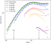 |
Fig. E.2. Analytical implementation of binning with pixels of size ℓ in the computation of the average structure function. The turbulent velocity field and the cluster emissivity of type Xbeta are both identical to Fig. D.3. Plain lines show exact results using the stationary, unbounded (R = ∞) velocity field, effectively replacing P2D by |

Finally, in addition to this “smoothing” effect, pixelisation induces a discretization effect, or “aliasing”. We do not develop a calculation for this effect. For a given two-dimensional frequency ωξ, aliasing arises for very specific combinations of separations s and pixel sizes, matching integer multiples of the associated spatial scales. It therefore strongly depends on the exact definition of the pixel grid. Since the power spectrum is continuous in the inertial range, aliasing effects are smoothly distributed across the range of separations s between the injection and dissipation scales. This aliasing effect is expected to mostly affect the structure function SF(s) at separations close to the dissipation and the injection scales, where significant discontinuities show up in the power spectrum.
Appendix F: Derivation of the variance of the structure function
F.1. General expression
Following similar notations, for a given pair indexed by i, we write ni = Np(si) and we introduce

We note in particular that
 (F.1)
(F.1)
Even in the case of an infinitely dense grid of pixels, there is a source of uncertainty arising from the stochastic nature of the velocity field itself. To see this more clearly, we compute
Neglecting border effects, ni = nj ∝ 2π𝒮𝒜. Therefore one writes
We stress that |ri| = si and that si and sj are not necessarily equal. Integration runs over all pairs indexed by i and j within the field. In a similar way to the one-dimensional case, we assume that
The decomposition of the product in brackets therefore involves six terms: bA, bB, bC, bD, bE, bF with bB = bC and bD = bE.
Computation of bA: It corresponds to the case in which  ,
,  and
and  . It is written
![Mathematical equation: $$ \begin{aligned} b_A&= (n_i n_j)^{-1} \sum _{\boldsymbol{\underline{k}} \ne \pm \boldsymbol{\underline{l}}} P_{\rm 3D}(k) P_{\rm 3D}(l) \int \left| C_{\boldsymbol{\theta }_i, \boldsymbol{r}_i}(\boldsymbol{\underline{k}}) \right|^2 \left| C_{\boldsymbol{\theta }_j, \boldsymbol{r}_j}(\boldsymbol{\underline{l}}) \right|^2 \\&= (n_i n_j)^{-1} \left[ \sum _{\boldsymbol{\underline{k}}} P_{\rm 3D}(k) I_{s_i}(\boldsymbol{\underline{k}}) \right] \left[ \sum _{\boldsymbol{\underline{l}}} P_{\rm 3D}(l) I_{s_j}(\boldsymbol{\underline{l}}) \right] \\&\qquad \qquad \qquad - 2 (n_i n_j)^{-1} \sum _{\boldsymbol{\underline{k}}}P_{\rm 3D}(k)^2 I_{s_i}(\boldsymbol{\underline{k}}) I_{s_j}(\boldsymbol{\underline{k}}). \end{aligned} $$](/articles/aa/full_html/2019/09/aa35676-19/aa35676-19-eq182.gif)
with Is already defined in Appendix D. Therefore, the first term is simply sf(si)sf(sj).
Computation of bB: It corresponds to the case in which  ,
,  and
and  . It is written
This involves the function
By developing the expression of Cθ, r and using Parseval’s theorem, we find
 (F.2)
(F.2)
Computation of bD: It corresponds to  . It is written
Computation of bF: It corresponds to  . It is written
Reassembling all terms together, we obtain the covariance term defined by

and which is written
![Mathematical equation: $$ \begin{aligned} \Sigma _{ij}&= \frac{1}{(2 \pi \mathcal{S} _{\mathcal{A} })^2} \left[ 2 \sum _{\boldsymbol{\underline{k}}, \boldsymbol{\underline{l}}} P_{\rm 3D}(k) P_{\rm 3D}(l) J_{s_i}(\boldsymbol{\underline{k}}, \boldsymbol{\underline{l}}) J_{s_j}^*(\boldsymbol{\underline{k}}, \boldsymbol{\underline{l}}) \right.\nonumber \\&\qquad \qquad \quad \left.- \sum _{\boldsymbol{\underline{k}}} R_{\boldsymbol{\underline{k}}} \times \left\{ 2 I_{s_i}(\boldsymbol{\underline{k}}) I_{s_j} (\boldsymbol{\underline{k}}) + J_{s_i}(\boldsymbol{\underline{k}}, \boldsymbol{\underline{k}}) J_{s_j}^*(\boldsymbol{\underline{k}}, \boldsymbol{\underline{k}}) \right\} \right] . \end{aligned} $$](/articles/aa/full_html/2019/09/aa35676-19/aa35676-19-eq194.gif) (F.3)
(F.3)
The expressions for I and J are given by Eqs. (D.2) and (F.2), respectively. Notably, the second term within brackets vanishes for Rayleigh-distributed coefficients. In principle, finite-sized corrections must also apply, like for the expected value of the structure function. We do not provide such corrections here and keep in mind that our variance estimate neglects border effects.
F.2. Case of an emissivity independent of the line of sight
The expression above can be further simplified if the emissivity is independent of the line-of-sight direction. Introducing  the Fourier transform of the analysis region and
  its power spectrum, we obtain
  . We define the following functions, whose principal interest resides in the fact that they only depend on the definition of the analysis region and can be precomputed numerically for any given instrumental field of view:
The normalisation constant is K = (ω/2π)2/𝒮𝒜 throughout this paper.
Using these functions, the variance is then written
 (F.4)
(F.4)
where we introduce  the 2D power spectrum of the centroid map over an infinitely extended domain (Appendix C) and
If the moduli are Rayleigh-distributed, it is evident that Q2D = 0 and the expression for the variance (Eq. (F.4)) depends only on the 2D power spectrum of the velocity. As already noted, the terms encapsulating the field-of-view geometry (𝒰𝒜, 𝒯𝒜) are factored out from the emissivity and turbulence part (P2D, Q2D).
Further simplification can be made when the analysis region is extremely wide compared to the separations s and to the largest fluctuation scale of the velocity map (still assuming a constant emissivity on sky). The limit 𝒜 → ∞ then applies and  becomes a strongly peaked function around 0. The above functions are rewritten as
The sign indicates the convolution product. Since 𝒜2 = 𝒜, we obtain
This automatically shows that 𝒯𝒜(ξ; s)=1 − J0(ωξs) and 𝒰𝒜(ξ, ξ; s)=0. Moreover,
Grouping terms together in Eq. (F.4) leads to Eq. (13).
Appendix G: Fourier transform of the normalised emissivity field ρ (spherical β-model)
We provide useful calculations for the 3D power spectrum of the normalised emissivity ρ in a case of a β-model. We also discuss the limiting case of very extended sources (equivalently, very small fields of view).
G.1. General case
Calculation of the two-dimensional power spectrum involves the calculation of  with ρ(x, θ)=ϵ(x, θ)/F(θ). As noted above (Appendix C), it is compulsory to fill ρ with zeros outside of its domain of definition or outside of the analysis domain. We consider here an arbitrarily large circular analysis domain 𝒜 (of radius R, centred on the source) to perform the following calculations.
Using the expression for F(θ) derived in a previous section (Eq. (B.1)), we obtain
The Fourier transform  is calculated in two steps. The integration over the x axis is performed first and its result is already displayed in Eq. (B.2). Integration over the second axis runs for all θ ∈ 𝒜 and we find
which uses the special integral defined below and represented in Fig. G.1 for n = 3/2 (β = 2/3):
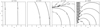 |
Fig. G.1. Numerical calculations of ℋp; n(u, v) for various values of p and n = 3/2. Logarithmically-spaced contours (identical in all panels, dashed lines for negative values) indicate the value of the function. This function is involved in the calculation of the Fourier transform of the normalised emissivity of a spherical β-model (n = 3β − 1/2) analysed over a concentric circular aperture of radius p times the core radius. The strong oscillatory behaviour is particularly noticeable in the last panel. |
recalling that ℱn(x)=xnKn(x).
G.2. Limit for small analysis domains (R ≪ rc)
If R/rc is small, those terms in  are approximatively constant under the integral and
![Mathematical equation: $$ \begin{aligned} P_{\rho } (k_x, \boldsymbol{\xi }) \simeq \frac{2^{3-6\beta }}{ \Gamma (3 \beta -1/2)^2} \left[ \mathcal{F} _{3\beta -1/2}\left( \omega |k_x| r_c \right) \right]^2 \times \left[ 2 \pi R^2 \frac{J_1(\omega \xi R)}{\omega \xi R} \right]^2\cdot \end{aligned} $$](/articles/aa/full_html/2019/09/aa35676-19/aa35676-19-eq212.gif)
The right-most factor involving the order 1 Bessel function J1 is the power spectrum of a circular pupil of radius R. Its integral over ξ equals πR2(2π/ω)2 and rapidly falls to zero for ω|ξ|≳3.83R−1. This result can easily be generalised to an analysis domain of arbitrary shape, introducing its power spectrum P𝒜,
 (G.1)
(G.1)
and we naturally recover the limiting case discussed several times in this paper where the emissivity ϵ(x, θ)=ϵ(x) does not depend on the line of sight θ over the analysis domain. Finally, R(≪rc) can still be very large and therefore  : the component of Pρ in the ξ plane can then be seen as a sharp low-pass filter; this corresponds to the case discussed in previous works (e.g. ZuHone et al. 2016).
Appendix H: Numerical validation results, continued
We show here the equivalent of Figs. 5, 6, 9, and 10 for the two other sets of 100 simulations (Table 1). All parameters remain the same apart from the injection scales, respectively Linj = 200 kpc (Figs. H.1–H.4) and Linj = 300 kpc (Figs. H.5–H.8). These comparisons still demonstrate a good match between the simulations and analytic results.
All Tables
Numerical realisations of a three-dimensional velocity cube used for validating the analytic calculations of line centroid shift, line broadening, and structure function sample variances.
All Figures
|
Fig. 1. One realisation of a uni-dimensional turbulent velocity field (middle panel) along the spatial axis x (in arbitrary units) with parameters α = 1/3, kmin = 1 (Linj = 2), kmax = 20 (Ldiss = 0.1), σturb = 160 km s−1, and σth = 100 km s−1 (shown by yellow shading). The emissivity profile (top panel) of the gas corresponds to a β density model with core radius rc = 0.2 and at a distance θ = 0.2 from the centre. The lower panel shows the resulting line profile as a thick black line. The best-fit Gaussian centred on C (vertical line) of width S is shown as a dashed red line. The green thin curve shows the Gaussian centred on the line centroid. Its width equals the geometrical mean of the thermal and turbulent broadening. |
| In the text | |
|
Fig. 2. Line centroid C versus line width (squared) S2 of an emission line along a single line of sight and 5000 realisations of a one-dimensional turbulent velocity field (σturb = 160 km s−1, kmin = 1, kmax = 20, σth = 100 km s−1). Left panel: assumes only random phases while the right panel also includes randomly distributed moduli (Rayleigh distribution). Points show measurements, and the red cross is the measured mean and standard deviations along both axes. The blue lines represent the results obtained from analytical calculations (Eqs. (4)–(7)). The plain green line shows the location of the geometric mean of the turbulent and thermal dispersions: the presence of turbulent motions on scales comparable to that of the cluster makes such an estimate a biased one. |
| In the text | |
|
Fig. 3. Effect of the finite box size on the precision of our numerical simulations. Three-dimensional velocity dispersion ΔV3D in each of the 100 numerical realisations for the three configurations in Table 1 is shown as blue histograms. Vertical dashed line indicates the exact value of σturb from integration of the input turbulent power-spectrum (Eq. (14)). The increased numerical dispersions in those values as Linj increases as a consequence of the finite simulation box size. |
| In the text | |
|
Fig. 4. Projection of a single realisation of a 3D velocity field (injection scale at 200 kpc) with several emissivity models (top row). All but the last column correspond to spherical β-models with core-radii of 4, 21, 54, 107, 215, and 429 kpc (from left to right). The rightmost column corresponds to a constant emissivity in the entire simulation box. The size of each panel is 520 kpc on a side. The middle row shows the centroid shift (C) and the bottom row shows the line width ( |
| In the text | |
|
Fig. 5. Numerical validation of Eqs. (8)–(11). These are the expected value and sample variance of the line centroid shift C𝒲 (first and second panel) and the expected value and sample variance of the line width |
| In the text | |
|
Fig. 6. Similar to Fig. 5 for a spherical β-model emissivity (beta). The numerical uncertainties are slightly larger (in the fourth panel, compared to Fig. 5) due to a lower accuracy in the numerical integration of Eq. (11). |
| In the text | |
|
Fig. 7. Sample variance associated to line measurements. The centroid shift (left) and broadening (right) in apertures of growing sizes for clusters presenting identical emissivity models are shown for a spherical β-model with core radius of 107 kpc. These curves are predicted analytically by Eqs. (9) and (11). They have been normalised to the value of the 3D turbulent velocity dispersion σturb. The different shapes of the curves as the aperture radius grows can be used as a diagnostic to discriminate between various injection scales. |
| In the text | |
|
Fig. 8. Comparison of numerical and analytical structure functions and their sample variance for various cluster sizes (i.e. various core radii (rc) of the β-model) and various pixel sizes (ℓ). The data points and thick error bars show the sample mean and standard deviation of the 100 realisations (individually represented as thin grey lines) for each of the considered configurations. The coloured curves and shaded areas represent the analytical calculations following Eqs. (12) and (13). The emissivity model is Xbeta and the region of analysis is a circle of diameter 520 kpc (as displayed in Fig. E.1). The turbulent power spectrum is that of Table 1 with an injection scale of 100 kpc. |
| In the text | |
|
Fig. 9. Representation of the absolute relative difference between the numerical and analytical estimates of the sample mean of the structure function, ⟨SF⟩, at three distinct separations s. Each coloured square corresponds to one experiment based on the same 100 realisations of the velocity field with Linj = 100 kpc and various binning sizes (y-axis) and β-models core radii (x-axis). Small red crosses indicate locations where the binning size is larger than s. |
| In the text | |
|
Fig. 10. Similar to Fig. 9, but for the sample variance of the structure function, Var(SF). Positive values indicate higher predicted variance compared to that measured in the numerical validation procedure. Although some of these numbers are high at face value, it is important to recall the assumptions leading to the chosen analytical formula and the noise inherent in our set of numerical simulations (see text). |
| In the text | |
|
Fig. 11. Comparison of the simulated and calculated structure function in a similar way as Fig. 8, except the emissivity model is of type beta (spherical β-model gas density). This induces non-stationarity of the projected velocity field, noticeable by the drop at large s. The coloured curves represent the analytical calculation of the mean structure function following Eqs. (12) and (D.3). For simplicity, the variance remains calculated according to Eq. (13), that is assuming Xbeta emissivity with an effective core radius, |
| In the text | |
|
Fig. 12. Model predictions for radial profiles of line properties, which are those measurements in spectra collected in circularly concentric annuli of equal width (21 kpc). The figure shows the sample variance of the centroid shift (left panel), the sample average of the line broadening (middle panel), and the sample variance of the line broadening. The injection scale is Linj = 100 kpc, and the emissivity model is a spherical β = 2/3 model with core radii indicated in legend. Shaded rectangles indicate bin widths (horizontally) and numerical uncertainties (vertically). |
| In the text | |
|
Fig. 13. Model predictions for structure functions and their associated sample variances under two instrumental setups: XRISM/Resolve (assuming 1.5′ resolution elements) and Athena/X-IFU (assuming 5″ and 15″ resolution elements for high and low signal-to-noise ratios respectively). Left panel: predictions for a ∼15′×15′ contiguous mapping of the Coma cluster while the right panel shows the result for a single X-IFU pointing. A single Resolve pointing (3′ on a side) would be too small for a useful derivation of the structure function. The text gives further details on the input turbulent power spectrum and gas density model. |
| In the text | |
|
Fig. B.1. Numerical calculations of ℐp; n(u, v) for various values of p and n = 3/2. Logarithmically-spaced contours (identical in all panels) indicate the value of the function. This function is involved in the calculation of the Fourier transform of a spherical β-model (n = 3β − 1/2) observed through a concentric circular aperture of radius p times the core radius. |
| In the text | |
|
Fig. D.1. Sketch illustrating the counting of pairs within a circular domain of analysis of radius R represented by the large black circle. Within this domain, the centroid shift C(θ) takes values determined by the stochastic turbulent field, while we set C = 0 outside. Counting inner pairs (shown with green and red sticks) separated by a distance s is performed by computing the range of accessible angles ϕs(θ) for a given position in the domain, then dividing by two. External pairs have only one end within the domain of analysis and the range of accessible angles is 2π − ϕs at a given position. |
| In the text | |
|
Fig. D.2. Counting pairs in the circular analysis region. Left: two-dimensional representation of the function ϕs(θ) for various values of the separation s and the position θ in a circular field of view of radius R. Right: scaling of Np(s), the number of pairs of points separated by a distance s within a circular field of view of radius R. “Inner” concerns those pairs integrally contained within the circular domain, while “Ext” concerns those pairs with only one end within the domain. “All” is the sum of the two numbers. The curves actually show δ(sNp(s))/δs, which is the differential number of pairs per interval of s expressed in units of the radius R. Here ℓ ≪ R is the side length of an elementary pixel, so that the total number of pixels in the circle is πR2/ℓ2. |
| In the text | |
|
Fig. D.3. Impact of finite-sized corrections on the mean structure functions computed according to our model. The domain of analysis is a circle of radius R. Both panels show the same data, in logarithmic or linear scales. The emissivity model is of type Xbeta with a core radius rc = 400 kpc. The turbulent power spectrum has injection and dissipation scales Linj and Ldiss respectively. The thick dashed line is barely visible and shows the exact result obtained assuming an infinitely extended analysis domain. Points at large separations s are subject to slight numerical instabilities. |
| In the text | |
|
Fig. E.1. Effect of a larger pixelisation when computing the structure function. Pixel size ranges from ℓ = 4, 17, 34, 69 kpc (from left to right). All four panels represent the same projected velocity field (injection scale at 100 kpc) in a galaxy cluster represented by a Xbeta model of core radius 21 kpc. In general, larger pixels reduce the power in the two-dimensional velocity fluctuations and roughly act like a smoothing convolution filter on the high-resolution centroid map. |
| In the text | |
|
Fig. E.2. Analytical implementation of binning with pixels of size ℓ in the computation of the average structure function. The turbulent velocity field and the cluster emissivity of type Xbeta are both identical to Fig. D.3. Plain lines show exact results using the stationary, unbounded (R = ∞) velocity field, effectively replacing P2D by |
| In the text | |
|
Fig. G.1. Numerical calculations of ℋp; n(u, v) for various values of p and n = 3/2. Logarithmically-spaced contours (identical in all panels, dashed lines for negative values) indicate the value of the function. This function is involved in the calculation of the Fourier transform of the normalised emissivity of a spherical β-model (n = 3β − 1/2) analysed over a concentric circular aperture of radius p times the core radius. The strong oscillatory behaviour is particularly noticeable in the last panel. |
| In the text | |
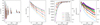 |
Fig. H.1. As Fig. 5 for the simulation with injection scale 200 kpc. |
| In the text | |
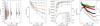 |
Fig. H.2. As Fig. 6 for the simulation with injection scale 200 kpc. |
| In the text | |
 |
Fig. H.3. As Fig. 9 for the simulation with injection scale 200 kpc. |
| In the text | |
 |
Fig. H.4. As Fig. 10 for the simulation with injection scale 200 kpc. |
| In the text | |
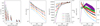 |
Fig. H.5. As Fig. 5 for the simulation with injection scale 300 kpc. |
| In the text | |
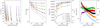 |
Fig. H.6. As Fig. 6 for the simulation with injection scale 300 kpc. |
| In the text | |
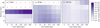 |
Fig. H.7. As Fig. 9 for the simulation with injection scale 300 kpc. |
| In the text | |
 |
Fig. H.8. As Fig. 10 for the simulation with injection scale 300 kpc. |
| In the text | |
Current usage metrics show cumulative count of Article Views (full-text article views including HTML views, PDF and ePub downloads, according to the available data) and Abstracts Views on Vision4Press platform.
Data correspond to usage on the plateform after 2015. The current usage metrics is available 48-96 hours after online publication and is updated daily on week days.
Initial download of the metrics may take a while.