| Issue |
A&A
Volume 679, November 2023
|
|
|---|---|---|
| Article Number | A87 | |
| Number of page(s) | 25 | |
| Section | The Sun and the Heliosphere | |
| DOI | https://doi.org/10.1051/0004-6361/202346615 | |
| Published online | 28 November 2023 | |
Assessment of the CRD approximation for the observer’s frame RIII redistribution matrix
1
Euler Institute, Università della Svizzera italiana (USI), East Campus, Sector D, Via la Santa 1, 6962 Lugano, Switzerland
e-mail: This email address is being protected from spambots. You need JavaScript enabled to view it.
2
Istituto ricerche solari Aldo e Cele Daccò (IRSOL), Faculty of Informatics, Università della Svizzera italiana (USI), Via Patocchi 57, 6605 Locarno, Switzerland
3
Institute for Computational and Mathematical Engineering, Stanford University, Center for Turbulence Research, Room 204, 481 Panama Mall, Stanford, CA 94305-3024, USA
4
Simula Research Laboratory, Kristian Augusts gate 23, 0164 Oslo, Norway
5
FernUni, Schinerstrasse 18, 3900 Brig, Switzerland
6
Leibniz-Institut für Sonnenphysik (KIS), Schöneckstrasse 6, 79104 Freiburg i. Br., Germany
Received:
7
April
2023
Accepted:
2
September
2023
Abstract
Context. Approximated forms of the RII and RIII redistribution matrices are frequently applied to simplify the numerical solution of the radiative transfer problem for polarized radiation, taking partial frequency redistribution (PRD) effects into account. A widely used approximation for RIII is to consider its expression under the assumption of complete frequency redistribution (CRD) in the observer’s frame (RIII−CRD). The adequacy of this approximation for modeling the intensity profiles has been firmly established. By contrast, its suitability for modeling scattering polarization signals has only been analyzed in a few studies, considering simplified settings.
Aims. In this work, we aim to quantitatively assess the impact and the range of validity of the RIII−CRD approximation in the modeling of scattering polarization.
Methods. We first present an analytic comparison between RIII and RIII−CRD. We then compare the results of radiative transfer calculations, out of local thermodynamic equilibrium, performed with RIII and RIII−CRD in realistic one-dimensional atmospheric models. We focus on the chromospheric Ca I line at 4227 Å and on the photospheric Sr I line at 4607 Å.
Results. The RIII−CRD approximation provides accurate results for the Ca I 4227 Å line. Only when velocities are included can some appreciable discrepancies be found, especially for lines of sight close to the disk center. The approximation performs well also for the Sr I 4607 Å line, especially in the absence of magnetic fields or when a micro-turbulent field is included. However, some appreciable errors appear when deterministic magnetic fields or bulk velocities are considered.
Conclusions. Our results show that the RIII−CRD approximation is suited for the PRD modeling of the scattering polarization signals of strong chromospheric lines, both in the core and wings. With a few minor exceptions, this approximation is also suitable for photospheric lines, although PRD effects generally play a minor role in their modeling.
Key words: radiative transfer / methods: numerical / polarization / scattering / stars: atmospheres / Sun: atmosphere
© The Authors 2023
 Open Access article, published by EDP Sciences, under the terms of the Creative Commons Attribution License (https://creativecommons.org/licenses/by/4.0), which permits unrestricted use, distribution, and reproduction in any medium, provided the original work is properly cited.
This article is published in open access under the Subscribe to Open model. This email address is being protected from spambots. You need JavaScript enabled to view it. to support open access publication.
1. Introduction
Significant scattering polarization signals are observed in several strong resonance lines of the solar spectrum, such as H I Ly-α (Kano et al. 2017), Mg II k (Rachmeler et al. 2022), Ca II K, Ca I 4227 Å, and Na I D2 (e.g., Stenflo et al. 1980; Stenflo & Keller 1997; Gandorfer 2000, 2002). These signals, which are characterized by broad profiles with large amplitudes in the line wings, encode a variety of information on the thermodynamic and magnetic properties of the upper layers of the solar atmosphere (e.g., Trujillo Bueno 2014; Trujillo Bueno et al. 2017). A correct modeling of these profiles requires solving the radiative transfer (RT) problem for polarized radiation in nonlocal thermodynamic equilibrium (non-LTE) conditions, taking partial frequency redistribution (PRD) effects (i.e., correlations between the frequencies of incoming and outgoing photons in scattering processes) into account (e.g., Faurobert-Scholl 1992; Stenflo 1994; Holzreuter et al. 2005; Belluzzi & Trujillo Bueno 2012).
A powerful formalism to describe PRD phenomena is that of the redistribution function (e.g., Hummer 1962; Mihalas et al. 1978), which is generalized to the redistribution matrix in the polarized case (e.g., Domke & Hubeny 1988; Stenflo 1994; Bommier 1997a,b). For resonance lines, the redistribution matrix is given by the sum of two terms, commonly labeled as RII and RIII according to the notation introduced by Hummer (1962). The RII matrix describes scattering processes that are coherent in frequency in the atomic reference frame, while RIII describes scattering processes that are totally incoherent in the same frame (e.g., Bommier 1997a,b)1. The linear combination of RII and RIII allows for frequency redistribution effects due to elastic collisions with neutral perturbers to be taken into account (e.g., Bommier 1997b). In the observer’s frame, the Doppler shifts due to the thermal motions of the atoms are responsible for further frequency redistribution effects. The Doppler effect actually induces a complex coupling between the frequencies and propagation directions of the incident and scattered radiation, which makes the evaluation of both RII and RIII, as well as the solution of the whole non-LTE RT problem, notoriously challenging from the computational standpoint. For this reason, approximate expressions of the redistribution matrices in the observer’s frame, in which such coupling is loosened, have been proposed and extensively used. In this context, a common choice is to use the angle-averaged (AA) expression of RII, hereafter RII−AA (e.g., Mihalas et al. 1978; Rees & Saliba 1982; Bommier 1997b; Leenaarts et al. 2012), and the expression of RIII obtained under the assumption that the scattering processes described by this matrix are also totally incoherent in the observer’s frame, hereafter RIII−CRD (e.g., Mihalas et al. 1978; Bommier 1997b; Alsina Ballester et al. 2017). The latter is also referred to as the assumption of complete frequency redistribution (CRD) in the observer’s frame.
The impact and the range of validity of the RII−AA approximation in the modeling of scattering polarization has been discussed by several authors (e.g., Faurobert 1987, 1988; Nagendra et al. 2002, 2020; Nagendra & Sampoorna 2011; Sampoorna et al. 2011, 2017; Anusha & Nagendra 2012; Sampoorna & Nagendra 2015; del Pino Alemán et al. 2020; Janett et al. 2021a). These studies have shown that the use of RII−AA can introduce significant (and hardly predictable) inaccuracies in the modeling of the line-core signals, while it seems to be suited for modeling the wing lobes and their magnetic sensitivity through the magneto-optical (MO) effects. By contrast, little effort has been directed to determine the suitability of the RIII−CRD assumption when modeling scattering polarization. Although this approximation has no true physical justification, it proved to be suitable for modeling the intensity profiles of spectral lines (e.g., Chap. 13 of Mihalas et al. 1978, and references therein). However, Bommier (1997b) pointed out that it may lead to appreciable errors when polarization phenomena are taken into account. In that work, the author considered a 90° scattering process of an unpolarized beam of radiation in the presence of a weak magnetic field, and compared the polarization of the scattered radiation calculated considering the exact expression of RIII and the RIII−CRD approximation, finding appreciable differences between the two cases2. The exact expression of RIII has been used in the non-LTE RT calculations with isothermal one-dimensional (1D) atmospheric models by Sampoorna et al. (2011) and Supriya et al. (2012) for the nonmagnetic case, Nagendra et al. (2002) and Supriya et al. (2013) in the weak field Hanle regime, and, more recently, Sampoorna et al. (2017) in the more general Hanle-Zeeman regime. In this last paper, the authors analyzed the suitability of the RIII−CRD approximation for modeling scattering polarization, considering an ideal spectral line. They first concluded that the use of RIII−CRD introduces some inaccuracies, especially in the line wings, when considering optically thin self-emitting slabs in the presence of weak magnetic fields (i.e., fields for which the ratio #x0393;B between the magnetic splitting of the Zeeman sublevels and the natural width of the upper level of the considered transition is on the order of unity). Moreover, these discrepancies are much smaller when stronger magnetic fields (#x0393;B ≈ 100) are considered (see Fig. 1 and Sect. 4 in Sampoorna et al. 2017). However, when considering an atmospheric model with a greater optical depth, they found that the use of RIII−CRD does not seem to produce any noticeable effect on the emergent Stokes profiles already for weak fields (see Fig. 2 in Sampoorna et al. 2017). To the best of the authors’ knowledge, the aforementioned works are the only ones reporting PRD calculations of scattering polarization performed using the exact expression of RIII.
Taking advantage of a new solution strategy for the non-LTE RT problem for polarized radiation, tailored for including PRD effects (see Benedusi et al. 2022), we provide a quantitative analysis of the suitability of the RIII−CRD approximation, considering more general and realistic settings than in previous studies. In particular, we show the results of non-LTE RT calculations of the scattering polarization signals of two different spectral lines (i.e., Ca I 4227 Å and Sr I 4607 Å) in 1D models of the solar atmosphere, both semi-empirical and extracted from 3D magneto-hydrodynamic (MHD) simulations, and accounting for the impact of realistic magnetic and bulk velocity fields.
The paper is structured as follows. Section 2 presents the basic equations for the RT problem for polarized radiation, as well as the redistribution matrix formalism for describing PRD effects. Section 3 briefly presents the discretization and algebraic formulation of the problem, together with the considered numerical solution strategy. Section 4 exposes analytical and numerical comparisons between RIII and RIII−CRD. Section 5 provides some general considerations on the role of RIII in the RT modeling of scattering polarization, and on the expected impact of RIII−CRD. Sections 6 and 7 report comparisons of non-LTE RT calculations of scattering polarization signals in realistic 1D settings, performed with RIII and RIII−CRD. Finally, Sect. 8 provides remarks and conclusions.
2. Transfer problem for polarized radiation
The intensity and polarization of a radiation beam are fully described by the four Stokes parameters I, Q, U, and V. The Stokes parameter I is the intensity, Q and U quantify the linear polarization, while V quantifies the circular polarization (e.g., Landi Degl’Innocenti & Landolfi 2004, hereafter LL04). The Stokes parameters and other physical quantities involved in the RT problem are generally functions of the frequency and propagation direction of the radiation beam under consideration, as well as of the spatial point and time. Hereafter, we assume stationary conditions so that all quantities are time-independent.
A beam of radiation propagating in a medium (e.g., the plasma of a stellar atmosphere) is modified as a result of the interaction with the particles therein and the possible presence of magnetic, electric, and bulk velocity fields. This modification is fully described by the RT equation for polarized radiation, consisting of coupled systems of first-order, inhomogeneous, ordinary differential equations. Defining the Stokes parameters as the four components of the Stokes vector I = (I, Q, U, V)T = (I1, I2, I3, I4)T ∈ ℝ4, the RT equation for a beam of radiation of frequency ν, propagating along the direction specified by the unit vector Ω = (θ, χ)∈[0, π]×[0, 2π) can be written as3
 (1)
(1)
where ∇Ω denotes the directional derivative along Ω, and r ∈ D is the spatial point in the domain D ⊂ ℝ3. The propagation matrix K ∈ ℝ4 × 4 is given by
 (2)
(2)
The elements of K describe absorption (η1), dichroism (η2, η3, and η4), and anomalous dispersion (ρ2, ρ3, and ρ4) phenomena. The emission vector ε = (ε1, ε2, ε3, ε4)T ∈ ℝ4 describes the radiation emitted by the plasma in the four Stokes parameters.
In this work, we consider the contribution to K and ε brought by both line and continuum processes. These contributions, labeled with the superscripts ℓ and c, respectively, simply add to each other:
In the frequency interval of a given spectral line, the line contribution to the elements of K and ε depends on the state of the atom (or molecule) giving rise to that line. In general, this state has to be determined by solving a set of rate equations (statistical equilibrium equations), which describe the interaction of the atom with the radiation field (radiative processes), other particles present in the plasma (collisional processes), and external magnetic and electric fields. When the statistical equilibrium equations have an analytic solution, the line contribution to the emission vector can be directly related to the radiation field that illuminates the atom (incident radiation) through the redistribution matrix formalism. More precisely, the line contribution to the emission vector can be written as the sum of two terms, namely,

where εℓ, sc describes the contribution from atoms that are radiatively excited (scattering term), and εℓ, th describes the contribution from atoms that are collisionally excited (thermal term). Following the convention that primed and unprimed quantities refer to the incident and scattered radiation, respectively, the line scattering term can be written through the scattering integral
 (3)
(3)
where the factor kL is the frequency-integrated absorption coefficient, and R ∈ ℝ4 × 4 the redistribution matrix. The redistribution matrix element Rij relates the emissivity in the ith Stokes parameter in direction Ω and frequency ν to the jth Stokes parameter of the incident radiation with direction Ω′ and frequency ν′.
In this work, we consider an atomic system composed of two-levels (two-level atom) with an unpolarized and infinitely sharp lower level (see Appendix for more details), and we apply the corresponding redistribution matrix as derived in Bommier (1997b):

The explicit expressions of RII and RIII in both the atomic and observer’s reference frames are given in Appendix B. The line contribution to the elements of the propagation matrix K, and the line thermal emissivity εℓ, th in the observer’s frame can be found in Appendix C. The continuum contribution to the emissivity can also be written as the sum of a thermal and a scattering term (see Eq. (D.1)), where the latter can be expressed as a scattering integral fully analogous to Eq. (3). A detailed discussion of the continuum terms is provided in Appendix D. For simplicity, hereafter we use the notation εth and εsc to refer to the thermal and scattering contributions to the emissivity, including both line and continuum.
The RT problem consists in finding a self-consistent solution for the RT equation (1) and the equation for the scattering contribution to the emissivity (3). This problem is in general nonlinear because of the factor kL appearing in the line contribution to both the elements of the propagation matrix and the emission coefficients. This factor is proportional to the population of the lower level, which in turn depends nonlinearly on the incident radiation field through the statistical equilibrium equations.
We linearize the problem with respect to I, by fixing a priori the population of the lower level, and thus the factor kL. In such scenario, whose suitability is discussed in Janett et al. (2021b) and Benedusi et al. (2021), the propagation matrix K and the thermal contribution to the emissivity εth is independent of I, while the scattering term εsc depends on it linearly through the scattering integral. The population of the lower level can be taken either from the atmospheric model (if provided) or from independent calculations. The latter can be carried out with available non-LTE RT codes that possibly neglect polarization (which is expected to have a minor impact on the population of ground or metastable levels), but allow considering multilevel atomic models. In this way, accurate estimates of the lower level population can be used, and reliable results can be obtained in spite of the simplicity of the considered two-level atomic model (e.g., Janett et al. 2021a; Alsina Ballester et al. 2021).
3. Numerical solution strategy
Following the works by Janett et al. (2021b) and Benedusi et al. (2021, 2022), we first present an algebraic formulation of the considered linearized RT problem for polarized radiation. Starting from this formulation, we then apply a parallel solution strategy, based on Krylov iterative methods with physics-based preconditioning. This strategy allows us to solve the problem in semi-empirical 1D models of the solar atmosphere, considering the exact expression of both RII and RIII redistribution matrices. The same approach, coupled with a new domain decomposition technique, has been recently generalized to the 3D case (Benedusi et al. 2023).
The problem presented in Sect. 2 is discretized by introducing suitable grids for the continuous variables r, Ω, and ν. The angular grid  is determined by the quadrature rule chosen to solve the angular integral in Eq. (3). We consider a right-handed Cartesian reference system with z-axis directed along the vertical. A given direction Ω is specified by the inclination θ and the azimuth χ, defined as shown in Fig. 1.
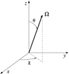 |
Fig. 1. Right-handed Cartesian reference system considered in the problem. The z-axis is directed along the local vertical. Any vector is specified through its polar angles θ (inclination) and χ (azimuth). |
We discretize the inclination through two Gauss-Legendre grids with Nθ/2 points each, one for μ = cos(θ)∈(−1, 0), and one for μ ∈ (0, 1). For the azimuth, we use a grid of Nχ equidistant points. The angular quadrature is then the spherical Cartesian product (e.g., Davis & Rabinowitz 2007) of the Gauss-Legendre rule for the inclination and the trapezoidal rule for the azimuth. This approach is commonly used in RT applications and allows for the implementation of fast algorithms. The frequency grid  is chosen to adequately sample the spectral line under investigation.
In a 1D (plane-parallel) setting, the spatial coordinate r = (x, y, z) can be replaced by the vertical coordinate z ∈ [zmin, zmax], and the RT equation (1) can be rewritten as
 (4)
(4)
The spatial grid  is provided by the considered atmospheric model. We assume that the radiation entering the atmosphere from the lower boundary is isotropic, unpolarized, and equal to the Planck function, and that no radiation is entering from the upper boundary. Equation (4) is thus equipped with the following boundary conditions:
![Mathematical equation: $$ \begin{aligned} \boldsymbol{I}\left(z_{\rm min},\theta ,\chi ,\nu \right)&= \left[ B_{P}\left(\nu , T(z_{\mathrm{min}}) \right), 0, 0, 0 \right]^T \quad \theta \in [0,\pi /2), \, \forall \chi , \, \forall \nu , \\ \boldsymbol{I}\left(z_{\rm max},\theta ,\chi ,\nu \right)&= \boldsymbol{0} \qquad \qquad \qquad \qquad \qquad ~\, \theta \in (\pi /2,\pi ], \, \forall \chi , \, \forall \nu , \end{aligned} $$](/articles/aa/full_html/2023/11/aa46615-23/aa46615-23-eq11.gif)
where BP is the Planck function and T the effective temperature. Given the propagation matrices and the emission vectors at all height points  , for a given direction (θ, χ) and frequency ν, the RT equation (1) can be numerically solved along that direction and at that frequency by applying a suitable integrator. This process is generally known as a formal solution. In this work, we use the L-stable DELO-linear method combined with a linear conversion to optical depth (e.g., Janett et al. 2017, 2018). An analysis of the stability properties of this method can be found in Janett & Paganini (2018).
With N = 4NzNθNχNν being the total number of unknowns, we introduce the collocation vectors  and
and  , which contain the numerical approximations of the Stokes vector and the emission vector, respectively, at all nodes. Given ϵ, the solution of all discretized RT equations (4) can be written as
 (5)
(5)
where Λ : ℝN → ℝN is the transfer operator, which encodes the formal solver and the propagation matrix, and  is a vector encoding the boundary conditions.
Similarly, given I, the discrete computation of the emission vector can be written as
 (6)
(6)
where ϵsc and ϵth encode the scattering and thermal contributions (including both line and continuum processes), respectively, as described in Sect. 2. The scattering operator Σ : ℝN → ℝN encodes the numerical evaluation of the scattering integral (3) and thus depends on the chosen numerical quadratures. In general, the operator Σ is given by the sum of different components, namely,
where ΣII and ΣIII encode the contributions from RII and RIII, respectively, and Σc the scattering contribution from the continuum. The vector ϵth ∈ ℝN encodes the thermal emissivity.
Under the assumption that kL is known a priori (see end of Sect. 2), the operators Λ and Σ are linear with respect to I. Combining Eq. (5) and Eq. (6), the whole discrete RT problem can be formulated as a linear system of size N with unknown I, namely
 (7)
(7)
where  is the identity matrix. The right-hand-side vector Λϵth + t can be computed a priori by solving Eq. (4) with thermal contributions only (i.e., by performing a single formal solution with ϵsc = 0). The action of the matrices Λ, Σ, and Id − ΛΣ can be encoded in a matrix-free form (see Benedusi et al. 2022).
We solve the linear system (7) by applying a matrix-free, preconditioned GMRES method, with a relative tolerance of 10−7. Preconditioning is performed by describing scattering processes in the limit of CRD. This corresponds to substituting the operator ΣII + ΣIII with a new operator ΣCRD that is much cheaper to evaluate. The explicit expression of ΣCRD for the considered atomic model can be found in Chap. 10 of LL04. The reader is referred to Benedusi et al. (2022) for more details on this solution strategy.
We conclude this section by briefly describing the numerical strategy used to handle bulk velocities. These velocities introduce Doppler shifts, which depend on the propagation direction of the considered radiation, in the expressions of the elements of K and ε (see Appendix B). We compute the emission vector in a reference frame in which the bulk velocity is zero (comoving reference frame). In this reference frame, there are no Doppler shifts, and this allows us to significantly reduce the number of evaluations of the redistribution matrix when performing the scattering integral (3). The drawback of this approach is that it requires transforming the incident radiation field from the observer’s frame to the comoving frame and then transforming the emission vector back to the observer’s frame. These steps are performed by means of high-order interpolations (e.g., cubic splines) on the frequency axis. The additional computational cost introduced by such interpolations is more than compensated by the reduced number of evaluations of the redistribution matrices.
4. Comparison of RIII and RIII−CRD
In this section, we first present an analytical comparison between the general angle-dependent expression of the RIII matrix (hereafter denoted as RIII) and its RIII−CRD approximation. We then review the reasons why the RIII−CRD approximation allows for a significant simplification of the problem from a computational point of view, and also provide a presentation of the challenges faced when considering RIII, focusing on algorithmic aspects.
4.1. Analytic considerations
In the formalism of the irreducible spherical tensors for polarimetry (see Chap. 5 of LL04), the RIII redistribution matrix in the observer’s reference frame (Eq. (B.29)) is given by the product between the scattering phase matrix  (Eq. (B.12)), which only depends on r, Ω, and Ω′, and the redistribution function
  (Eq. (B.30)), which also depends on ν and ν′. This factorization also holds for the RIII−CRD matrix, leaving the
  matrix unchanged, while replacing the redistribution function
  with the approximation
  given by Eq. (B.35). A fundamental difference between
  and
and  is that the former depends on the scattering angle Θ = arccos(Ω ⋅ Ω′) (i.e., the angle between the directions Ω and Ω′), while the latter does not.
To analyze the dependence on Θ, we start considering the simpler expressions that  and
and  assume in the absence of magnetic fields (B = 0). In this case, the magnetic shifts uMuMℓ (see Eq. (B.20)) are zero, and the sums over the magnetic quantum numbers M appearing in Eqs. (B.30) and (B.36) can be performed analytically. If we additionally assume that there are no bulk velocities (vb = 0) or, without loss of generality, we evaluate the redistribution matrix in the comoving frame (see Sect. 3), the Doppler shifts ub (see Eq. (B.20)) also vanish, and the dependence on the propagation directions Ω and Ω′ is only through the scattering angle Θ. Expressing the functions in terms of the reduced frequencies u and u′ (see Eq. (B.19)), in the limit of B = 0 and vb = 0, one finds:
![Mathematical equation: $$ \begin{aligned} \mathcal{R} ^{{\scriptscriptstyle \mathrm{III}},KK^{\prime }}_Q (\boldsymbol{r},\boldsymbol{\Omega },\boldsymbol{\Omega }\prime ,u,u^\prime ) \xrightarrow [B=0,\,{ v}_b=0] \delta _{KK^{\prime }} \, \tilde{\mathcal{R} }^{{\scriptscriptstyle \mathrm{III}},K} (\boldsymbol{r},\Theta ,u,u^\prime ), \end{aligned} $$](/articles/aa/full_html/2023/11/aa46615-23/aa46615-23-eq30.gif)
with
 (8)
(8)
The quantities βK and α are given by Eqs. (B.3) and (B.4), respectively, in the limit of no magnetic fields, while WK is defined as (see Eq. (10.17) of LL04)
where Jℓ and Ju are the total angular momenta of the lower and upper level, respectively, and the operator in curly brackets is the Wigner’s 6-j symbol. The quantity  takes different analytical forms depending on the value of Θ:
-
if Θ ∈ (0, π) (i.e., if Ω′≠Ω, −Ω)
 (9)
(9) -
if Θ = 0 (i.e., forward scattering Ω′=Ω)
 (10)
(10)and
-
if Θ = π (i.e., backward scattering Ω′= − Ω)
 (11)
(11)
In the previous equations, H is the Voigt profile (i.e., the real part of the Faddeeva function, see Chap. 5 of LL04) and ϕ the Lorentzian profile (i.e., the real part of the function φ defined in Eq. (B.28)). Similarly, it can be shown that
![Mathematical equation: $$ \begin{aligned} \mathcal{R} ^{{\scriptscriptstyle \mathrm{III-CRD}},KK^{\prime }}_Q(\boldsymbol{r},\boldsymbol{\Omega },\boldsymbol{\Omega }\prime ,u,u^\prime ) \xrightarrow [B=0,\,{ v}_b=0] \delta _{KK^{\prime }} \, \tilde{\mathcal{R} }^{{\scriptscriptstyle \mathrm{III-CRD}},K}(\boldsymbol{r},u,u^\prime ), \end{aligned} $$](/articles/aa/full_html/2023/11/aa46615-23/aa46615-23-eq37.gif)
with
Recalling that the Voigt profile is, by definition, a convolution between a Gaussian and a Lorentzian distribution (e.g., Chap. 5 of LL04), from Eq. (9), it can be easily seen that for Θ = π/2
This shows that the approximate  function corresponds to the exact
  for Θ = π/2, namely,
 (12)
(12)
For scattering angles Θ ≠ π/2, the functions  and
and  are generally different, and this difference increases as Θ approaches the two limiting cases of forward and backward scattering (i.e., Θ = 0 and Θ = π, respectively). This can be clearly seen in Fig. 2, where
  is plotted as a function of u′ for different values of u and Θ. In particular, we compare the profiles for Θ = 0 and π, to that of Θ = π/2, which, as shown above, corresponds to
  . For any value of u, the function
  shows a relatively broad profile (full width at half maximum of about 2), centered at u′ = 0. The amplitude of the peak is maximum at u = 0 (left panel) and quickly decreases by various orders of magnitude already at u ≈ 3 (middle panel). The behavior of the function
  is much more complex. For u = 0 (left panel) and Θ = 0 or π, the profile is centered at u′ = 0 and it is much sharper and with a larger amplitude than that of
  . For u ≈ 3 (middle panel) and Θ = 0 (resp. Θ = π), the function is characterized by a broad profile, similar in amplitude and width to that of Θ = π/2 (which is equivalent to
  , see Eq. (12)), but with its maximum slightly shifted to positive (resp. negative) values of u′. Additionally, it shows a secondary sharp peak centered at u′=u (resp. u′= − u). For u ≈ 9 (right panel), in the case of Θ = 0 (resp. Θ = π), the secondary peak becomes negligible, while the main one is very similar to that of
  . Noting that the dependence on K is limited to the factors βK and WK (see Eq. (8)), it is possible to state that
  and
and  are de facto equivalent in the wings, independently of the value of Θ. By contrast, they differ in the core and near wings, where the magnitude of the discrepancies strongly depends on Θ.
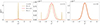 |
Fig. 2. Comparison of |

In the presence of a magnetic field, the redistribution function  (Eq. (B.30)) is given by a linear combination of the functions
  (Eqs. (B.31)–(B.33)). These functions are fully analogous to
  (Eqs. (9)–(11)), the only difference being that the second and third functions in the integrand (i.e., the profiles depending on the scattered and incident radiation, respectively) are shifted by uMuMℓ and
  , respectively. It can be shown that also in the presence of magnetic fields (but still neglecting bulk velocities), the following relation holds:

When Θ ≠ π/2,  (as function of u′) differs in general from
  . As in the unmagnetized case, the difference is marginal for large values of u (i.e., u > 6) independently of the magnetic field strength, while it can be very significant in the core and near wings, especially when Θ is close to 0 or π. When approaching these limit cases, the curves for
  can show very sharp peaks and the contribution of the various Zeeman components, split in frequency by the magnetic field, can eventually be resolved. As an illustrative example, Fig. 3 shows the component
  plotted as a function of u′, for u = 0.76, B = 30 G, and different values of Θ. We note that this component has a nonzero imaginary part since Q ≠ 0. As for the unmagnetized case, the curve for Θ = π/2, which corresponds to the CRD approximation, shows a broad profile centered at u′ = 0. As Θ departs from π/2, the corresponding profiles show increasingly large differences from the previous one. In particular, for Θ approaching 0 (resp. π), the position of the maximum moves from u′ = 0 toward u′=u (resp. u′= − u), while the width of the profile becomes sharper and the amplitude larger, in both the real and imaginary parts. As the profiles become sharper, the Zeeman components become visible, producing small lobes of opposite signs with respect to the central peak in the real part (left panels) and small substructures in the central peak in the imaginary part (right panels).
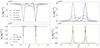 |
Fig. 3. Real (left column) and imaginary (right column) parts of |

In summary, the RIII−CRD approximation should be suitable in the far wings of the spectral lines (see right panel of Fig. 2), while it can introduce inaccuracies in the core and near wings, mainly due to scattering processes with Θ close to 0 or π, for which RIII−CRD and RIII differ significantly.
4.2. Computational considerations on RIII−CRD
The RIII−CRD approximation is based on the assumption that scattering processes are totally incoherent also in the observer’s frame, which in turn implies that in a scattering event, absorption and reemission can be treated as completely independent processes. Consistently with this picture, Eq. (B.35) shows that in RIII−CRD the joint probability of absorbing radiation with frequency ν′ and reemitting radiation with frequency ν is simply given by the product of two generalized profiles  (Eq. (B.36)). Following the approach discussed at the end of Sect. 3, we evaluate the emission vector in the comoving frame, where no bulk velocities are present. In this case, the generalized profiles do not depend on the propagation directions Ω and Ω′, and from Eqs. (B.29), (B.35), and (B.12), one finds that the emission coefficients corresponding to RIII−CRD are given by
 (13)
(13)
where i = 1, …, 4, Kmin = min(K, K′), and #x0394;νD,  , and
, and  are the Doppler width (in frequency units), the polarization tensor, and the rotation matrices, respectively (see Appendix B for more details). Finally,
  is the radiation field tensor, defined as (see Eq. (5.157) of LL04)
Equation (13) shows that the dependencies on the frequency and propagation direction of the incoming and outgoing radiation are completely decoupled. This allows the implementation of simple and fast computational algorithms: once the values of  are obtained from the formal solution of the RT equation, it is possible to independently compute the values of
  for the frequencies of the incoming and outgoing radiation and combine them only during the final calculation of the emission coefficient. Using the big-O notation, the time complexity (e.g., Sipser 1996) of the algorithm scales as O
 , where d ∈ (1, 2) grows monotonically with Nν. For the typical size of the frequency grids needed to synthesize one (or a few) spectral lines (i.e., Nν ≈ 100), d can be considered close to 1. This kind of time complexity is justified because the calculation of the generalized profile is slow (complex algorithms are required), while the subsequent combination of them is fast as it only implies products of complex numbers.
In numerical applications considering the RIII−CRD approximation, it is a common practice to perform the integration over the frequencies of the incoming radiation in Eq. (13) using the frequency grid from the problem discretization (see Sect. 3) without further refinements, and applying the trapezoidal rule. This methodology has the advantages of a decreased time-to-solution (TTS) and implementation simplicity. On the other hand, it should be pointed out that the accuracy of the results can be improved by using denser and more specific grids for the frequencies of the incoming radiation without any major loss of overall performance. This is because, even if a finer frequency grid is used in Eq. (13), in a PRD setting the TTS for evaluating the total emissivity remains mainly dominated by the contribution of the angle-dependent RII redistribution matrix.
4.3. Computational considerations on RIII
The evaluation of εIII considering the exact expression of RIII (see equations in Appendix B.2.2) is computationally challenging for the following main reasons: (a) it involves a 4-dimensional integration, leading to a very large number of evaluations of the integrands in Eqs. (B.31)–(B.33). This issue is otherwise known as the curse of dimensionality; (b) the integration variables (ν′, Ω′, and y) cannot be algebraically decoupled; (c) already for simple atomic transitions, the total number of combinations of magnetic quantum numbers coupled with the tensorial polarimetric indices is high, which adds another layer of complexity to the 4 dimensions of the overall problem; (d) the integrands include the Faddeeva function (Faddeeva & Terent’ev 1961) whose evaluation requires a large TTS (e.g., Oeftiger et al. 2016; e) the integrands show a very complex behavior with respect to the various integration variables and parameters, thus requiring the use of very fine, unstructured, and case-dependent grids.
Our overall approach for calculating εIII is to first evaluate the integral over y, followed by that over the frequencies ν′, and finally, the one over the propagation direction Ω′. The analytic expressions of ℐ (Eqs. (B.31)–(B.33)) show that in the absence of bulk velocities (or if the redistribution matrix is evaluated in the comoving frame), the coupling between the propagation directions of the incoming and outgoing radiation occurs through the scattering angle Θ. The integrand in ℐ shows a complex behavior with respect to the integration variable y, especially when the scattering angle approaches 0 and π. In these cases, the integrand becomes close to a Lorentz distribution or its square. These functions are not easy to numerically integrate due to the presence of sharp peaks and extended wings. Indeed, the convergence rate for the numerical quadrature of the Lorentz distribution (and its square) is generally slow. Furthermore, the computation of a single ℐ (see Eq. (B.31)) can require up to thousands of evaluations of the Faddeeva function (accounting for more than 70% of the TTS). In order to perform the quadratures over y, we applied an adaptive quadrature method based on the Gauss-Kronrod approach (e.g., Kronrod 1965; Piessens et al. 2012). The advantage of this method is that it is capable of automatically inferring the behavior of the integrand by achieving very high accuracy with a relatively low number of function evaluations.
In general, the time complexity for the computation of εIII is O . The cubic contribution given by the number of frequency grid points is due to the fourth dimension induced by y. It must be noted that the number of grid points needed to adequately perform the quadrature of the integral over y is generally larger than Nν.
For the angular integral in Eq. (3), it is convenient to apply a quadrature rule characterized by a regular angular grid, because in this case, the effective number of different scattering angles is significantly lower than the total pairs of directions. The results reported in the next sections were obtained with the quadrature method described in Sect. 3, with 12 Gauss-Legendre inclinations and 8 equally spaced azimuths. In this case, the total number of scattering angles is limited to 200. In our algorithm, the quantities ℐ are precomputed for the whole set of different scattering angles corresponding to the chosen angular grid, thus avoiding repeating the calculation of ℐ, which is rather expensive, for different pairs of directions having the same scattering angle.
The quantity ℐ depends on two pairs of magnetic quantum numbers, (Mu, Mℓ) and  , where the labels u and ℓ indicate the upper and lower level, respectively. Equation (B.30) shows that the expression of RIII actually includes four quantities ℐ, which differ for the values of the magnetic quantum numbers and are coupled inside six nested loops over such quantum numbers. It can be easily realized that in such loops several tuples of magnetic sublevels are repeated, which suggests the opportunity to increase the efficiency of the algorithm by precomputing the quantities ℐ for all possible combinations of magnetic quantum numbers, thus avoiding to recalculate the same quantity ℐ various times. The precomputation of ℐ as described above leads to a drastic reduction of the total number of calculations needed to compute εIII, which otherwise would be very significant due to the extra dimension in the integration. The precomputed values of ℐ are stored out-of-core (e.g., on disk) because they require a large footprint, and are accessed during the calculation of εIII through a system of look-up tables. It must be observed that the quantity ℐ and, consequently, the grids used for performing the numerical integration, also depends on the spatial point through the damping parameter a, the magnetic field, and the Doppler width #x0394;νD. Our strategy thus calls for relatively large data storage capabilities that, however, remain manageable in the case of 1D applications.
5. Impact of RIII on spectral lines formation
The RIII redistribution matrix describes scattering processes during which the atom undergoes elastic collisions with neutral perturbers (mainly hydrogen and helium atoms in the solar atmosphere) that completely relax any correlation between the frequencies of the incident and scattered radiation, thus making the scattering totally incoherent. Informally speaking, due to such collisions, the atom does not keep any memory of the frequency of the incident photon. On the contrary, the RII redistribution matrix describes scattering processes in which the atom is not subject to any elastic collisions so that the frequencies of the incident and scattered radiation remain fully correlated (coherent scattering). A quantitative estimate of the relative weight of RIII with respect to RII is provided by the branching ratio for RII (see Eq. (B.9)) in the absence of magnetic fields (a.k.a. coherence fraction):
where Auℓ is the Einstein coefficient for spontaneous emission, Cuℓ is the rate of inelastic de-exciting collisions, and Qel is the rate of elastic collisions with neutral perturbers. A value of  close to unity (corresponding to a very low rate of elastic collisions compared to the rates for spontaneous emission and collisional de-excitation) means that RII dominates over RIII, while a value of
  close to zero (corresponding to a very high value of Qel compared to Auℓ and Cuℓ) means instead that RIII dominates with respect to RII.
The impact of RIII is thus expected to be marginal in the core of strong spectral lines (i.e., lines showing broad intensity profiles with extended wings). Indeed, their line-core radiation generally originates from the upper layers of the solar atmosphere, where the number density of neutral perturbers (and thus the rate of elastic collisions) is relatively low. The relative weight of RIII can, however, become significant in the wings of such lines, as they usually form much lower in the atmosphere. On the other hand, it must be observed that the profiles entering the definition of RIII are all centered around the line-center frequency, and therefore the net contribution of this redistribution matrix to the emissivity in the line wings is generally marginal with respect to that of RII. This can be seen as an analytical proof of the well-known fact that scattering processes are mainly coherent in the line wings (e.g., Mihalas et al. 1978). Consistently with this picture, Alsina Ballester et al. (2022) showed that in the wings of strong resonance lines, the contribution of RIII needs to be taken into account in order not to overestimate the weight of RII, but its net contribution to scattering polarization is fully negligible. These considerations suggest that the exact analytical form of RIII should not be crucial for modeling the core and far wings of strong lines, and that the RIII−CRD approximation should therefore be suitable in these spectral ranges. The most critical regime is that of the near wings, where strong resonance lines may show very significant scattering polarization signals. There, RIII may bring a non-negligible contribution, and it is harder to estimate a priori the suitability of the RIII−CRD approximation.
The relative weight of RIII is also non-negligible in the case of spectral lines forming in the deeper layers of the solar atmosphere (photosphere), where the number density of colliders is significant. On the other hand, these lines are generally weak in the intensity spectrum, showing narrow absorption profiles with a Doppler core and no wings. Since Doppler redistribution is generally very efficient in the line-core, the limit of CRD (i.e., to assume that all scattering processes are totally incoherent) has always been considered a good approximation for modeling both the intensity (e.g., Mihalas et al. 1978) and scattering polarization profiles of these lines (e.g., LL04).
In order to quantitatively verify these considerations, and assess the suitability of the RIII−CRD approximation for modeling scattering polarization, we model the intensity and polarization of two different spectral lines, namely a strong spectral line with extended wings forming in the upper layers of the solar atmosphere, and a weaker line forming deeper in the atmosphere. Excellent examples for these two typologies of spectral lines are, respectively, the Ca I line at 4227 Å and the Sr I line at 4607 Å. Both lines result from a resonant transition between the ground level of the considered atomic species, which in both cases has total angular momentum Jℓ = 0, and an excited level with Ju = 1. Both of them show conspicuous scattering polarization signals, which can be suitably modeled considering a two-level atom with an unpolarized and infinitely-sharp lower level.
Figure 4 shows the variation of the coherence fraction  with height in the 1D semi-empirical model C of Fontenla et al. (1993, hereafter FAL-C) for the two considered spectral lines. In the same figure, we also plot the height at which the optical depth τ, in the frequency intervals of the considered spectral lines, is unity. It can be shown (e.g., Mihalas et al. 1978) that this height provides an approximate estimate of the atmospheric region from which the emergent radiation originates (formation height). We recall that the optical depth at the frequency ν along direction Ω is defined as
 (14)
(14)
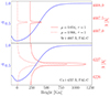 |
Fig. 4. Height variation of |

where s is the spatial coordinate along direction Ω (measured with respect to an arbitrary initial point), and η1 is the absorption coefficient for the intensity (see also Janett et al. 2017). For calculating the formation height, the direction Ω must point inward in the atmosphere, and the initial point s = 0 is taken at the upper boundary. Since the absorption coefficient is largest at the line center and decreases moving to the wings, it can be immediately seen that the formation height is highest in the line core and decreases moving to the wings. From Eq. (14) it is also clear that, for a given frequency, the formation height is higher for a line of sight (LOS) close to the edge of the solar disk (limb) than for one at the disk center. Clearly, the formation height is higher for strong lines which have a large absorption coefficient (because the number density of atoms in the lower level of the transition is particularly large in the solar atmosphere) than for weak ones.
5.1. Ca I 4227 Å line
In the intensity spectrum, the Ca I 4227 Å line shows a very broad and deep absorption profile (e.g., Gandorfer 2002) with an equivalent width of 1426 mÅ (Moore et al. 1966), that is, one of the strongest spectral lines in the visible part of the solar spectrum. When observed in quiet regions close to the limb, this line shows a large scattering polarization signal with a sharp peak in the line core and broad lobes in the wings (e.g., Gandorfer 2002). This signal, with its peculiar triplet-peak structure, has been extensively observed and modeled in the past (e.g., Stenflo et al. 1980; Faurobert-Scholl 1992; Bianda et al. 2003; Sampoorna et al. 2009; Anusha et al. 2011; Supriya et al. 2014; Carlin & Bianda 2017; Alsina Ballester et al. 2018; Janett et al. 2021a; Jaume Bestard et al. 2021, and references therein). In particular, it was clearly established that its broad wing lobes are produced by coherent scattering processes with PRD effects. We recall that the line-core peak is sensitive to the presence of magnetic fields via the Hanle effect. The Hanle critical field (i.e., the magnetic field strength for which the sensitivity to the Hanle effect is maximum) is Bc ≈ 25 G. The wing lobes are sensitive to longitudinal magnetic fields of similar strength via the magneto-optical (MO) effects (Alsina Ballester et al. 2018).
The lower panel of Fig. 4 shows that in the FAL-C atmospheric model, the core of the Ca I 4227 Å line forms above 800 km (low chromosphere). At these heights, the number density of neutral perturbers is very low, the coherence fraction is thus very close to unity, and RII dominates with respect to RIII. On the other hand, as we move from the core to the wings, the formation height quickly decreases to photospheric levels. At these heights, the coherence fraction is much lower than one and the weight of RIII is significant. On the other hand, for the reasons discussed above, its net impact in the line wings is expected to be relatively low. The most critical region is that of the near wings, where the Ca I 4227 Å line shows strong scattering polarization signals, and the net contribution from RIII can be non-negligible. The suitability of the RIII−CRD approximation in this spectral region can only be assessed numerically, and it will be analyzed in Sect. 6.
5.2. Sr I 4607 Å line
The Sr I 4607 Å line is a rather weak absorption line in the intensity spectrum, with an equivalent width of 36 mÅ only (see Moore et al. 1966). Nonetheless, this line shows a prominent scattering polarization signal at the solar limb, characterized by a sharp profile (e.g., Gandorfer 2002). This signal has been also extensively observed and modeled in the past, especially in order to investigate, via the Hanle effect, the small-scale, unresolved magnetic fields that permeate the quiet solar photosphere (e.g., Stenflo & Keller 1997; Trujillo Bueno et al. 2004; del Pino Alemán et al. 2018; del Pino Alemán & Trujillo Bueno 2021; Dhara et al. 2019; Zeuner et al. 2020, 2022). The Hanle critical field for this line is Bc ≈ 23 G. The limit of CRD has always been considered suited for modeling both the intensity and scattering polarization profiles of this line.
The upper panel of Fig. 4 shows that in the FAL-C atmospheric model, the core of this line forms in the photosphere, below 500 km. The curve for the coherence fraction shows that the weight of RIII is, as expected, significant at these heights. In the next section, we explore the suitability of the RIII−CRD approximation in the modeling of the scattering polarization signal of this line through full PRD RT calculations in the presence of both deterministic and nondeterministic (e.g., Stenflo 1982, 1994; Landi Degl’Innocenti & Landolfi 2004) magnetic fields. For the latter, we consider unimodal micro-structured isotropic (MSI) magnetic fields, namely magnetic fields with a given strength and an orientation that changes on scales below the mean free path of photons, uniformly distributed over all directions. The expressions of RT quantities in the presence of MSI magnetic fields are exposed in Appendix E (see also Sect. 4 of Alsina Ballester et al. 2017).
6. Numerical results: FAL-C atmospheric model
In this section and in the next one, we present the numerical results4 of non-LTE RT calculations of the scattering polarization profiles of the Ca I 4227 Å and Sr I 4607 Å lines, performed with the numerical solution strategy described in Sect. 3. All calculations are performed using the general (angle-dependent) expression of the RII redistribution matrix, while considering both the exact form of the RIII matrix and its RIII−CRD approximation. The lower level population, which we keep fixed in the problem (see the end of Sect. 2), is precomputed with the RH code (Uitenbroek 2001), which solves the nonlinear unpolarized non-LTE RT problem. For the Ca I 4227 Å line, we run RH using a model for calcium composed of 25 levels, including 5 levels of Ca II and the ground level of Ca III. For the Sr I 4607 Å line, we considered a model composed of 34 levels, including the ground level of Sr II. These preliminary computations also provided the rates for elastic and inelastic collisions, as well as the continuum quantities.
For a quantitative comparison between the emergent Stokes profiles obtained using RIII and RIII−CRD, we plot the error defined by
 (15)
(15)
where a and b represent the values of a given Stokes parameter of the emergent radiation, for a given direction and all considered wavelengths, obtained considering RIII and RIII−CRD, respectively. The maximum is calculated with respect to wavelength, over the considered interval. The error definition in Eq. (15) does not correspond to the standard relative error and it was introduced to prevent amplifying the discrepancies where a and b are close to zero and consequently to the numerical noise. Where the signals a and b are relevant, this definition provides a value that is smaller, by a factor of two in the worst case (i.e., where a takes its maximum value), than the usual relative error. This definition is thus justified as it provides the correct order of magnitude of the error where the signal is relevant while damping it when the signal becomes negligible.
In this section, we show calculations performed in the FAL-C atmospheric model (Nz = 70 height nodes), in the presence of constant (i.e., height-independent) deterministic magnetic fields (i.e., magnetic fields having a well-defined strength and orientation at each spatial point), in the absence of bulk velocity fields. The LOS toward the observer is taken on the x − z plane of the considered reference system (see Fig. 1) and is specified by μ = cos θ, with θ the inclination with respect to the vertical. Typically, we present the emergent Stokes profiles for two specific directions: μ = 0.034, which represents radiation coming from the solar limb (nearly horizontal LOS), and μ = 0.996, which represents radiation coming from near the center of the solar disk (nearly vertical LOS).
6.1. Ca I 4227 Å line
We first consider the modeling of the Stokes profiles of the Ca I 4227 Å line, which is discretized with Nν = 99 unevenly spaced nodes. The characteristics of this spectral line are adequately reproduced by our calculations. The triple-peak structure in Q/I is evident in the non-magnetized model shown in Fig. 5, while the magnetized case shown in Fig. 6 displays a clear depolarization of the core as a result of the Hanle effect and a mild depolarization of the lobes due to the magneto-optical effects.
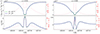 |
Fig. 5. Emergent Stokes I (top panels) and Q/I (bottom panels) profiles of the Ca I 4227 Å line at μ = 0.034 (left panels) and μ = 0.966 (right panels) calculated in the FAL-C atmospheric model in the absence of magnetic fields. Calculations take into account PRD effects considering the exact expression of RIII (blue lines) and the RIII−CRD approximation (green marked lines). The reference direction for positive Q is taken parallel to the limb. The red dotted lines report the error between RIII and RIII−CRD calculations, given by Eq. (15). |
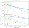 |
Fig. 6. Emergent Stokes I (first row), Q/I (second row), U/I (third row), and V/I (fourth row) profiles for the Ca I 4227 Å line at μ = 0.034 (left column) and μ = 0.966 (right column) calculated in the FAL-C atmospheric model in the presence of a horizontal (θB = π/2, χB = 0) magnetic field with B = 20 G. Calculations take into account PRD effects considering the exact expression of RIII (blue lines) and the RIII−CRD approximation (green marked lines). The reference direction for positive Q is taken parallel to the limb. The red dotted lines report the error between RIII and RIII−CRD calculations, given by Eq. (15). |
Figure 5 shows the Stokes I and Q/I profiles for a non-magnetic scenario, where we observe no significant difference between RIII and RIII−CRD calculations, with an error that is always smaller than 7.5 × 10⁻³. In the absence of magnetic fields, the U/I and V/I profiles vanish and are consequently not shown.
Figure 7 shows the contributions from RII, RIII, and RIII−CRD to |εI| and |εQ| for the non-magnetized case as a function of height. For the sake of completeness, the figure also shows the contributions from continuum and line thermal emissivities to Stokes I and from continuum to Stokes Q (see blue lines). In this figure, we consider μ = 0.17 and λ = 4227.1 Å, which corresponds to the wavelength at the maximum of the red Q/I lobe in Fig. 5 (left bottom panel). The limit of the gray region represents the height where the optical depth at the considered wing wavelength and LOS is unity. The top panel of Fig. 7 shows that the contributions to εI from RIII and RIII−CRD practically coincide at all heights, and that at the height where the optical depth is unity, they are very similar to that from RII. By contrast, in the bottom panel, we see that the contribution to εQ of RII dominates over that of RIII at all heights, and it can be thus considered the only relevant contributor to the formation of the Q/I wing lobe. In this case, the contribution from RIII−CRD is different from that of RIII, but it remains negligible with respect to that of RII. This explains why the computations of Fig. 5 do not show any appreciable differences between RIII and RIII−CRD in the line wings.
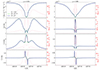 |
Fig. 7. Various contributions (see legend) to the emission coefficients for the Stokes parameters I (top panel) and Q (bottom panel) as a function of height in the FAL-C model, in the absence of magnetic fields. The emission coefficients are evaluated at the wavelength λ = 4227.1 Å, corresponding to the maximum of the Q/I lobe in the red wing of the line, for a LOS with μ = 0.17. The shaded area in the panels highlights the atmospheric region where the optical depth at this wavelength and LOS is greater than 1. εX (where X= I or Q) is the total emissivity, |


Finally, Fig. 6 displays all the Stokes profiles in the presence of a height-independent, horizontal magnetic field with B = 20 G. An overall good agreement between RIII and RIII−CRD settings is observed in all profiles. We note that the error is generally larger in the core and near wings of the Q/I, U/I, and V/I profiles. This conclusion remains valid for magnetic fields ranging from 10 G to 200 G. Indeed, these results show no significant differences and are therefore not reported.
6.2. Sr I 4607 Å line
We now consider the modeling of the Sr I 4607 Å line, which is discretized with Nν = 130 unevenly spaced nodes. Our non-LTE RT calculations adequately reproduce this weak line, showing a small absorption profile in the intensity spectrum without wings, and a prominent and sharp Q/I scattering polarization peak (see Fig. 8).
In the I and Q/I profiles shown in Fig. 8 for a non-magnetic scenario, we only note minor differences between RIII and RIII−CRD calculations. By contrast, we note some relevant discrepancies between RIII and RIII−CRD cases when a deterministic magnetic field is considered. Figures 9–11 display the Q/I, U/I, and V/I profiles in the presence of a height-independent, horizontal magnetic field with B = 20 G, B = 50 G, and B = 100 G, respectively. We omit to report the intensity I profiles, because they are essentially identical to those exposed in Fig. 8 for the non-magnetized case. We first note that, in all cases, there are no observable discrepancies between RIII and RIII−CRD calculations in the U/I and V/I profiles. By contrast, some relevant differences appear in the Q/I profiles, such as the one shown in the top-left panel of Fig. 10. Moreover, RIII−CRD calculations generally present larger Q/I line-core signals at μ = 0.966 with respect to RIII ones. For completeness, Fig. 12 displays the Q/I profile where we observed the maximal error, corresponding to the B = 20 G case at μ = 0.83.
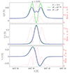 |
Fig. 12. Same as Fig. 9, but for μ = 0.83. In this Q/I profile, we observed the maximal error between RIII and RIII−CRD calculations. |
It is worth observing that for μ = 0.966 and a magnetic field with B = 20 G (i.e., a forward scattering Hanle effect geometry), the Ca I 4227 Å line shows a positive Q/I peak (see Fig. 6), while the Sr I 4607 Å line a negative one (see Fig. 9). Bearing in mind that both spectral lines originate from a Jℓ = 0 → Ju = 1 transition and have similar Hanle critical fields, we may suggest that this inversion is due to their different formation heights and properties. An in-depth analysis of this result goes beyond the scope of this paper and will be the object of a future investigation.
As anticipated, the Sr I 4607 Å line has been extensively exploited to investigate the small-scale unresolved magnetic fields that fill the quiet solar photosphere. For this reason, we have also analyzed the case of unimodal MSI magnetic fields. We recall that in the presence of such magnetic fields, the signatures of Zeeman and magneto-optical effects vanish due to cancellation effects, and the only impact of the magnetic field is the depolarization of Q/I due to the Hanle effect, which depends on the field strength. Figure 13 shows the I and Q/I profiles for a height-independent MSI magnetic field with B = 20 G. No significant differences between RIII and RIII−CRD calculations are visible, and the error is always smaller than 5 × 10⁻³. This result suggests that the RIII−CRD approximation provides accurate results when the problem is characterized by cylindrical symmetry, while it can introduce appreciable discrepancies when the direction of a non-vertical, deterministic magnetic field breaks this symmetry.
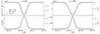 |
Fig. 13. Same as Fig. 8, but in the presence of a uniform micro-structured isotropic magnetic field with B = 20 G. |
7. Numerical results: 1D atmospheric model from 3D MHD simulation
In Sect. 6, we limited our calculations to the semi-empirical FAL-C atmospheric model, possibly including spatially uniform magnetic fields, in the absence of bulk velocities. In this section, we compare the impact of RIII and RIII−CRD in PRD calculations in a 1D atmospheric model extracted from a 3D MHD simulation, which includes height-dependent magnetic and bulk velocity fields. As we have seen in previous sections, the magnetic field impacts the polarization profiles through the Hanle, magneto-optical, and Zeeman effects. On the other hand, bulk velocities introduce Doppler shifts as well as amplitude enhancements and asymmetries in the polarization profiles (e.g., Sampoorna & Nagendra 2015, 2016; Carlin et al. 2012, 2013; Jaume Bestard et al. 2021). The joint impact of height-dependent magnetic fields and bulk velocities, together with the inherent thermodynamic structure of the atmospheric model, results in complex emergent Stokes profiles, in which it is generally difficult to distinguish the contribution of each factor.
In this work, we adopted a 1D atmospheric model extracted from the 3D magnetohydrodynamic (MHD) simulation of Carlsson et al. (2016), performed with the Bifrost code (Gudiksen et al. 2011). In practice, we took a vertical column of such 3D simulation, clipped in the height interval between −100 and 1400 km, which includes the region where the considered spectral lines form, discretized with Nz = 79 nodes. The corresponding vertical resolution ranges between 19 km and 100 km. Figure 14 shows the variation of the magnetic field, temperature, and vertical component of the bulk velocity as a function of height in the considered model (hereafter, Bifrost model), which shows relatively quiet conditions. Since the 1D module of the RH code (used to calculate the lower-level population) can only handle vertical bulk velocities, in this study we only considered the vertical component of the model’s velocity, although our code can in principle take into account velocities of arbitrary direction. As additional information, Fig. 15 shows the variation of the coherence fraction  with height in the Bifrost model for the two considered spectral lines, as well as the height at which the optical depth τ, in the frequency intervals of the two spectral lines, is unity (see Sect. 5).
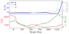 |
Fig. 14. Physical quantities of the considered 1D atmospheric model extracted from the 3D MHD Bifrost simulation en024048_hion (snapshot 385, column 120 × 120). Upper panel: strength (blue solid line), inclination (gray dashed line), and azimuth (light-blue dashed-dotted line) of the magnetic field as a function of height. Lower panel: vertical component of bulk velocity (green solid line) and temperature (red solid line) as a function of height. We adopt the convention that the velocity is positive if pointing outward in the atmosphere and negative if pointing inward. For clarity, the horizontal green dotted line indicates zero velocity. |
7.1. Ca I 4227 Å line
We first consider the modeling of the Ca I 4227 Å line, which is now discretized with Nν = 141 unevenly spaced nodes. Figure 16 displays all the Stokes profiles, showing an overall good agreement between RIII and RIII−CRD calculations for a LOS with μ = 0.034. By contrast, for a LOS with μ = 0.996, we observe some appreciable discrepancies in the Q/I and U/I profiles, with an error up to 3 × 10⁻¹. We recall that these linear scattering polarization signals, obtained for a LOS close to the disk center, are due to the forward-scattering Hanle effect (e.g., Trujillo Bueno 2001). Interestingly, such discrepancies disappear in the absence of bulk velocities (profiles not reported here). This suggests that the differences between RIII and RIII−CRD calculations are amplified in the presence of bulk velocities, and they are larger for a LOS close to the vertical because in this case the Doppler shifts are more pronounced. We finally note that the error affects the amplitudes of the main peaks of the profiles but not their shape.
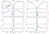 |
Fig. 16. Emergent Stokes profiles for the Ca I 4227 Å line calculated in the Bifrost model (see Sect. 7), which includes height-dependent magnetic and (vertical) bulk velocity fields. The vertical gray lines show the line-center wavelength in the absence of bulk velocities. |
7.2. Sr I 4607 Å line
We now consider the modeling of the Sr I 4607 Å line, which is discretized with Nν = 141 unevenly spaced nodes. First, we note that in this Bifrost model, this line shows an emission profile in intensity for a LOS of μ = 0.034. We verified that this is due to the thermodynamic structure of this atmospheric model, and it can be explained from the behavior of the source function at the formation height of the line for this limb LOS (see Fig. 15). Figure 17 shows that appreciable discrepancies between RIII and RIII−CRD calculations are found in all Stokes profiles for μ = 0.034, and in Q/I and U/I for μ = 0.966. The maximal error is found in the U/I profile at μ = 0.966, where however the polarization signal is very weak and thus of limited practical interest. The discrepancies between RIII and RIII−CRD computations become slightly larger in the Bifrost model, where also a bulk velocity field is included. On the other hand, observing that the most significant errors appear in very weak polarization signals, we can conclude that for practical applications the RIII−CRD approximation can be safely used to obtain reliable results.
8. Conclusions
In this work, we assessed the suitability and range of validity of a widely used approximation for RIII, that is, its expression under the assumption of CRD in the observer’s frame, labeled with RIII−CRD. To this aim, we solved the full non-LTE RT problem for polarized radiation in 1D models of the solar atmosphere, considering both the exact expression of RIII and its RIII−CRD approximation. With respect to the previous work of Sampoorna et al. (2017), we considered semi-empirical models, as well as 1D models extracted from 3D MHD simulations, which provide a reliable approximation of the solar atmosphere. The analysis was focused on the chromospheric Ca I line at 4227 Å and the photospheric Sr I line at 4607 Å, accounting for the impact of magnetic fields (both deterministic and micro-structured) and bulk velocities.
We first compared the analytical forms of RIII and RIII−CRD, showing that they correspond when the scattering angle Θ is equal to π/2, while their difference increases as Θ approaches 0 (forward scattering) or π (backward scattering). The numerical results for the Ca I 4227 Å line show that the RIII−CRD approximation is suited to model the scattering polarization signals of strong chromospheric lines. This is not surprising considering that in these lines the contribution of RII dominates with respect to that of RIII, both in the core (which forms high in the atmosphere) and in the far wings (where scattering is basically coherent). On the other hand, we verified that the RIII−CRD approximation is also adequate in the near wings, where the contribution of RIII cannot be neglected a priori. The numerical results for the Sr I 4607 Å line show that the RIII−CRD approximation also provides reliable results in photospheric lines, for which the contribution of RIII is significant. Observing that the scattering polarization signal of the Sr I 4607 Å line is extensively used to investigate the small-scale magnetic fields that fill the quiet solar photosphere, we verified that the RIII−CRD approximation is also suitable in the presence of micro-turbulent magnetic fields. On the other hand, some appreciable discrepancies (i.e., relative errors larger than 0.01 according to the error definition (15)) are found when deterministic magnetic fields or bulk velocities are included, and the polarization signals are below 0.4%. However, the qualitative agreement between the two settings remains satisfactory in general; differences in the overall shapes and signs are exceptions and appear when the signals are very weak. These discrepancies may suggest that the limit of CRD (i.e., to fully neglect PRD effects), which is generally adopted to model the intensity and polarization of these weak lines, can possibly introduce some appreciable inaccuracies with respect to a PRD treatment. A quantitative comparison between PRD and CRD calculations for this line is ongoing, and it will be presented in a separate publication.
In conclusion, we can state that in optically thick media, the use of the lightweight RIII−CRD approximation guarantees reliable results in the modeling of scattering polarization in strong and weak resonance lines.
In this work, the terms coherent and totally incoherent are used in the sense that the frequencies of the incident and scattered radiation are fully correlated and completely uncorrelated, respectively.
It must be observed that the author applied the CRD approximation after introducing in RIII other simplifications suited for the weak-field regime (see Sect. 4 of Bommier 1997b).
The azimuth is defined in the half-open interval χ = [0, 2π) because it has a periodicity of 2π and the two limits refer to the same coordinate.
All calculations involving RIII (in its angle-dependent formulation) were performed on the Piz Daint supercomputer of the Swiss National Supercomputing Center (CSCS) on Cray XC40 nodes (https://www.cscs.ch/computers/piz-daint). An XC40 compute node is equipped with two Intel®Xeon®E5-2695 v4 microprocessors at 2.10 GHz (2×18 cores, 64/128 GB RAM).
In the cgs system, the Larmor frequency is numerically approximated by νL = 1.3996 × 10⁶ B, with B expressed in G and νL in s−1.
Variable and index renaming for Eqs. (49) and (51) in Bommier (1997b):

For notational simplicity, the ranges of the various sums are not explicitly indicated.
Acknowledgments
We thank the anonymous referee for carefully reading the manuscript and for many useful comments, suggestions, and corrections. The financial support by the Swiss National Science Foundation (SNSF) through grant CRSII5_180238 is gratefully acknowledged.
References
- Alsina Ballester, E., Belluzzi, L., & Trujillo Bueno, J. 2017, ApJ, 836, 6 [Google Scholar]
- Alsina Ballester, E., Belluzzi, L., & Trujillo Bueno, J. 2018, ApJ, 854, 150 [Google Scholar]
- Alsina Ballester, E., Belluzzi, L., & Trujillo Bueno, J. 2021, Phys. Rev. Lett., 127, 081101 [NASA ADS] [CrossRef] [Google Scholar]
- Alsina Ballester, E., Belluzzi, L., & Trujillo Bueno, J. 2022, A&A, 664, A76 [NASA ADS] [CrossRef] [EDP Sciences] [Google Scholar]
- Anusha, L. S., & Nagendra, K. N. 2012, ApJ, 746, 84 [NASA ADS] [CrossRef] [Google Scholar]
- Anusha, L. S., Nagendra, K. N., Bianda, M., et al. 2011, ApJ, 737, 95 [NASA ADS] [CrossRef] [Google Scholar]
- Belluzzi, L., & Trujillo Bueno, J. 2012, ApJ, 750, L11 [NASA ADS] [CrossRef] [Google Scholar]
- Benedusi, P., Janett, G., Belluzzi, L., & Krause, R. 2021, A&A, 655, A88 [NASA ADS] [CrossRef] [EDP Sciences] [Google Scholar]
- Benedusi, P., Janett, G., Riva, S., Krause, R., & Belluzzi, L. 2022, A&A, 664, A197 [NASA ADS] [CrossRef] [EDP Sciences] [Google Scholar]
- Benedusi, P., Riva, S., Zulian, P., et al. 2023, J. Comput. Phys., 479, 112013 [NASA ADS] [CrossRef] [Google Scholar]
- Bianda, M., Stenflo, J., Gandorfer, A., & Gisler, D. 2003, Current Theoretical Models and Future High Resolution Solar Observations: Preparing for ATST (San Francisco: Astronomical Society of the Pacific), 286, 61 [NASA ADS] [Google Scholar]
- Bommier, V. 1997a, A&A, 328, 706 [NASA ADS] [Google Scholar]
- Bommier, V. 1997b, A&A, 328, 726 [NASA ADS] [Google Scholar]
- Carlin, E. S., & Bianda, M. 2017, ApJ, 843, 64 [NASA ADS] [CrossRef] [Google Scholar]
- Carlin, E. S., Manso Sainz, R., Asensio Ramos, A., & Trujillo Bueno, J. 2012, ApJ, 751, 5 [NASA ADS] [CrossRef] [Google Scholar]
- Carlin, E. S., Asensio Ramos, A., & Trujillo Bueno, J. 2013, ApJ, 764, 40 [NASA ADS] [CrossRef] [Google Scholar]
- Carlsson, M., Hansteen, V. H., Gudiksen, B. V., Leenaarts, J., & De Pontieu, B. 2016, A&A, 585, A4 [NASA ADS] [CrossRef] [EDP Sciences] [Google Scholar]
- Davis, P. J., & Rabinowitz, P. 2007, Methods of Numerical Integration (Courier Corporation) [Google Scholar]
- del Pino Alemán, T., Trujillo Bueno, J., Štěpán, J., & Shchukina, N. 2018, ApJ, 863, 164 [CrossRef] [Google Scholar]
- del Pino Alemán, T., Trujillo Bueno, J., Casini, R., & Manso Sainz, R. 2020, ApJ, 891, 91 [CrossRef] [Google Scholar]
- del Pino Alemán, T., & Trujillo Bueno, J. 2021, ApJ, 909, 180 [CrossRef] [Google Scholar]
- Dhara, S. K., Capozzi, E., Gisler, D., et al. 2019, A&A, 630, A67 [NASA ADS] [CrossRef] [EDP Sciences] [Google Scholar]
- Domke, H., & Hubeny, I. 1988, ApJ, 334, 527 [NASA ADS] [CrossRef] [Google Scholar]
- Faddeeva, V. N., & Terent’ev, N. M. 1961, Tables of Values of the Function W(z) (Pergamon Press) [Google Scholar]
- Faurobert, M. 1987, A&A, 178, 269 [NASA ADS] [Google Scholar]
- Faurobert, M. 1988, A&A, 194, 268 [NASA ADS] [Google Scholar]
- Faurobert-Scholl, M. 1992, A&A, 258, 521 [NASA ADS] [Google Scholar]
- Fontenla, J. M., Avrett, E. H., & Loeser, R. 1993, ApJ, 406, 319 [Google Scholar]
- Gandorfer, A. 2000, The Second Solar Spectrum: A high SpectralResolution Polarimetric Survey of Scattering Polarization at the Solar Limb in Graphical Representation. Volume I: 4625, Å to 6995 Å (Zurich: vdf ETH) [Google Scholar]
- Gandorfer, A. 2002, The Second Solar Spectrum: A high SpectralResolution Polarimetric Survey of Scattering Polarization at the Solar Limb in Graphical Representation. Volume II: 3910 Å to 4630 Å (Zurich: vdf ETH) [Google Scholar]
- Gudiksen, B. V., Carlsson, M., Hansteen, V. H., et al. 2011, A&A, 531, A154 [NASA ADS] [CrossRef] [EDP Sciences] [Google Scholar]
- Holzreuter, R., Fluri, D. M., & Stenflo, J. O. 2005, A&A, 434, 713 [NASA ADS] [CrossRef] [EDP Sciences] [Google Scholar]
- Hummer, D. G. 1962, MNRAS, 125, 21 [Google Scholar]
- Janett, G., & Paganini, A. 2018, ApJ, 857, 91 [Google Scholar]
- Janett, G., Carlin, E. S., Steiner, O., & Belluzzi, L. 2017, ApJ, 840, 107 [NASA ADS] [CrossRef] [Google Scholar]
- Janett, G., Steiner, O., & Belluzzi, L. 2018, ApJ, 865, 16 [NASA ADS] [CrossRef] [Google Scholar]
- Janett, G., Alsina Ballester, E., Guerreiro, N., et al. 2021a, A&A, 655, A13 [NASA ADS] [CrossRef] [EDP Sciences] [Google Scholar]
- Janett, G., Benedusi, P., Belluzzi, L., & Krause, R. 2021b, A&A, 655, A87 [NASA ADS] [CrossRef] [EDP Sciences] [Google Scholar]
- Jaume Bestard, J., Trujillo Bueno, J., Štěpán, J., & del Pino Alemán, T. 2021, ApJ, 909, 183 [NASA ADS] [CrossRef] [Google Scholar]
- Kano, R., Trujillo Bueno, J., Winebarger, A., et al. 2017, ApJ, 839, L10 [NASA ADS] [CrossRef] [Google Scholar]
- Kronrod, A. S. 1965, Nodes and Weights of Quadrature Formulas: sixteen-place Tables (New York: Consultants Bureau) [Google Scholar]
- Landi Degl’Innocenti, E., & Landolfi, M. 2004, Polarization in Spectral Lines (Springer Science& Business Media), 307 [Google Scholar]
- Leenaarts, J., Pereira, T., & Uitenbroek, H. 2012, A&A, 543, A109 [NASA ADS] [CrossRef] [EDP Sciences] [Google Scholar]
- Mihalas, D. 1978, Stellar Atmospheres, 2nd ed. (W. H. Freeman& Co.) [Google Scholar]
- Moore, C. E., Minnaert, M. G. J., & Houtgast, J. 1966, The Solar Spectrum 2935 A to 8770 A, Monograph (US: National Bureau of Standards), 61 [Google Scholar]
- Nagendra, K. N., & Sampoorna, M. 2011, A&A, 535, A88 [NASA ADS] [CrossRef] [EDP Sciences] [Google Scholar]
- Nagendra, K. N., Frisch, H., & Faurobert, M. 2002, A&A, 395, 305 [NASA ADS] [CrossRef] [EDP Sciences] [Google Scholar]
- Nagendra, K. N., Sowmya, K., Sampoorna, M., Stenflo, J. O., & Anusha, L. S. 2020, ApJ, 898, 49 [NASA ADS] [CrossRef] [Google Scholar]
- Oeftiger, A., Aviral, A., De Maria, R., et al. 2016, Proc. of International Particle Accelerator Conference (IPAC’16), Busan, Korea, May 8–13, 2016 (Geneva, Switzerland: JACoW), 3090 [Google Scholar]
- Piessens, R., de Doncker-Kapenga, E., Überhuber, C. W., & Kahaner, D. K. 2012, Quadpack: a Subroutine Package for Automatic Integration (Springer Science& Business Media), 1 [Google Scholar]
- Rachmeler, L. A., Trujillo Bueno, J., McKenzie, D. E., et al. 2022, ApJ, 936, 67 [NASA ADS] [CrossRef] [Google Scholar]
- Rees, D. E., & Saliba, G. J. 1982, A&A, 115, 1 [NASA ADS] [Google Scholar]
- Sampoorna, M., & Nagendra, K. N. 2015, ApJ, 812, 28 [CrossRef] [Google Scholar]
- Sampoorna, M., & Nagendra, K. N. 2016, ApJ, 833, 32 [NASA ADS] [CrossRef] [Google Scholar]
- Sampoorna, M., Stenflo, J. O., Nagendra, K. N., et al. 2009, ApJ, 699, 1650 [Google Scholar]
- Sampoorna, M., Nagendra, K. N., & Frisch, H. 2011, A&A, 527, A89 [NASA ADS] [CrossRef] [EDP Sciences] [Google Scholar]
- Sampoorna, M., Nagendra, K. N., & Stenflo, J. O. 2017, ApJ, 844, 97 [NASA ADS] [CrossRef] [Google Scholar]
- Sipser, M. 1996, Introduction to the Theory of Computation (USA: Cengage Learning) [Google Scholar]
- Stenflo, J. 1994, Solar Magnetic Fields: Polarized Radiation Diagnostics (Springer), 189 [CrossRef] [Google Scholar]
- Stenflo, J. O. 1982, Sol. Phys., 80, 209 [Google Scholar]
- Stenflo, J. O., & Keller, C. U. 1997, A&A, 321, 927 [NASA ADS] [Google Scholar]
- Stenflo, J. O., Baur, T. G., & Elmore, D. F. 1980, A&A, 84, 60 [NASA ADS] [Google Scholar]
- Supriya, H. D., Nagendra, K. N., Sampoorna, M., & Ravindra, B. 2012, MNRAS, 425, 527 [NASA ADS] [CrossRef] [Google Scholar]
- Supriya, H. D., Sampoorna, M., Nagendra, K. N., Ravindra, B., & Anusha, L. S. 2013, J. Quant. Spectr. Rad. Transf., 119, 67 [NASA ADS] [CrossRef] [Google Scholar]
- Supriya, H. D., Smitha, H. N., Nagendra, K. N., et al. 2014, ApJ, 793, 42 [Google Scholar]
- Trujillo Bueno, J. 2001, in Advanced Solar Polarimetry– Theory, Observation, and Instrumentation, ed. M. Sigwarth, ASP Conf. Ser., 236, 161 [Google Scholar]
- Trujillo Bueno, J. 2014, in Solar Polarization 7, eds. K. N. Nagendra, J. O. Stenflo, Z. Q. Qu, & M. Sampoorna, ASP Conf. Ser., 489, 137 [Google Scholar]
- Trujillo Bueno, J., Shchukina, N., & Asensio Ramos, A. 2004, Nature, 430, 326 [Google Scholar]
- Trujillo Bueno, J., Landi Degl’Innocenti, E., & Belluzzi, L. 2017, Space Sci. Rev., 210, 183 [CrossRef] [Google Scholar]
- Uitenbroek, H. 2001, ApJ, 557, 389 [Google Scholar]
- Zeuner, F., Manso Sainz, R., Feller, A., et al. 2020, ApJ, 893, L44 [NASA ADS] [CrossRef] [Google Scholar]
- Zeuner, F., Belluzzi, L., Guerreiro, N., Ramelli, R., & Bianda, M. 2022, A&A, 662, A46 [NASA ADS] [CrossRef] [EDP Sciences] [Google Scholar]
Appendix A: Atomic model and data
We consider an atomic system composed of two levels (two-level atom). Each level is characterized by the energy E, the quantum number for the total angular momentum J (positive integer or semi-integer values only), and the Landé factor g. Hereafter, the physical quantities referring to the upper and lower levels will be labeled with subscripts u and ℓ, respectively. Each level is composed of 2J + 1 magnetic sublevels characterized by the magnetic quantum number M (M = −J, −J + 1, ..., J). The magnetic sublevels are degenerate in the absence of magnetic fields, while they split in energy when a magnetic field B is present (Zeeman effect). Their energies are given by E(M) = EJ + h νL g M, where EJ is the energy of the considered J-level, h the Planck constant, and νL = eB(4πmec)−1 (with e the elementary charge, me the electron mass, and c the speed of light) the Larmor frequency5. The line-center frequency is ν0 = (Eu − Eℓ)/h. The frequency of the Zeeman component corresponding to the transition between the upper magnetic sublevel Mu and the lower magnetic sublevel Mℓ is

The energies, angular momenta, Landé factors, and Einstein coefficients for spontaneous emission Auℓ for the two-level atomic models considered in this work to synthesize the intensity and polarization of the Ca I 4227 Å and Sr I 4607 Å lines are summarized in Table A.1. The Landé factors of levels with Jℓ = 0 are formally taken to be zero.
Spectral lines and corresponding atomic data.
Appendix B: Redistribution matrix
All the results presented in this work are obtained considering the redistribution matrix for a two-level atom with an unpolarized and infinitely sharp lower level, in the presence of magnetic fields, as derived by Bommier (1997b). This redistribution matrix is given by the sum of two terms, commonly referred to as RII and RIII (e.g., Hummer 1962). In this appendix, we provide their analytic expressions, written with a slightly different notation than the one used in the original paper or in subsequent works in which the same redistribution matrices were reported and applied (e.g., Alsina Ballester et al. 2017). We first present their expressions in the atomic reference frame, taking the quantization axis along the magnetic field (Sect. B.1). We briefly comment on the branching ratios (Sect. B.1.1) and we derive their expressions in a new reference system with the quantization axis along the vertical (Sect. B.1.2). Subsequently, we transform them in the observer’s reference frame, including bulk velocities (Sect. B.2). Finally, we provide their expressions under a series of simplifying approximations, including the one for RIII analyzed in this work (Sect. B.3).
B.1. Expression in the atomic reference frame
In the atomic reference frame, taking the quantization axis parallel to the magnetic field (magnetic reference system), the RII and RIII redistribution matrices are respectively given by Eqs. (51) and (49) in Bommier (1997b). We refer to these redistribution matrices with the symbol  (with X = II,III) to distinguish them from those expressed taking the quantization axis along a different direction. After some variable and index renaming,6 we rewrite them in the following equivalent form
 (B.1)
(B.1)
where r is the spatial point, Ω the propagation direction, and ξ the radiation frequency in the atomic reference frame. The convention that primed and unprimed quantities refer to the incident and scattered radiation, respectively, is used. The indices i and j can take values 1, 2, 3, and 4, while Kmin = min(K, K′). The quantity  (with K = 0, ..., 2 and Q = −K, ..., K) is the geometrical tensor defined in Sect. 5.11 of LL04, evaluated in the magnetic reference system. Given that the direction of the magnetic field may vary with the spatial point, this tensor depends in general on r.
The function  is given by (see Eq. (49) of Bommier 1997b)
 (B.2)
(B.2)
where
 (B.3)
(B.3)
and
 (B.4)
(B.4)
The quantities #x0393;R, #x0393;I, and #x0393;E are the line broadening constants due to radiative decays, inelastic collisions, and elastic collisions, respectively:

where Cuℓ is the rate of inelastic collisions inducing transitions from the upper to the lower level and Qel is the rate of elastic collisions with neutral perturbers (mainly hydrogen and helium atoms). The quantity D(K) is the depolarizing rate due to elastic collisions. In the absence of experimental data or detailed theoretical calculations for the rates D(K), the approximate relation D(2) = 0.5 Qel is generally used. Under the assumption that the interaction between the atom and the perturber is described by a single tensor operator of rank K′, the rates with K ≠ 2 can be obtained from D(2) as discussed in Sect. 7.13 of LL04 (see equation after (7.108) and Eq. (7.109), which relates D(1) and D(2) for the case of K′ = 2). The generalized profile  is given by Eq. (10.40) of LL04 and can be equivalently written as
![Mathematical equation: $$ \begin{aligned} \Phi ^{KK^{\prime }}_Q \left( \boldsymbol{r},\xi \right) = \sum _{M_u,M_u^{\prime }=-J_u}^{J_u} \sum _{M_\ell =-J_\ell }^{J_\ell } \sum _{q,q^{\prime }=-1}^1 \mathcal{B} _{K K^{\prime } Q M_u M_u^{\prime } M_\ell q q^{\prime }} \, \frac{1}{2} \, \left[ \Phi _{M_u M_\ell }(\boldsymbol{r},\xi ) + \overline{\Phi }_{M_u^{\prime } M_\ell }(\boldsymbol{r},\xi ) \right] \, , \end{aligned} $$](/articles/aa/full_html/2023/11/aa46615-23/aa46615-23-eq100.gif) (B.5)
(B.5)
where K = 0, ..., 2Ju, K′ = 0, 1, 2, and Q = −Kmin, ..., Kmin with Kmin = min(K, K′). The notation  refers to the complex conjugate function. The quantity ℬKK′QMuMu′Mℓqq′ is given by
where the quantities in parentheses are the Wigner’s 3-j symbols (e.g., Sect. 2.2 of LL04). It must be observed that the 3-j symbols are nonzero only if the sum of the arguments of the lower raw is zero. Because of this, the values of q and q′ are uniquely determined once Mu,  , and Mℓ are assigned. Thus, the sums over these indices in Eq. (B.5) are in practice redundant. The complex profile ΦMuMℓ is defined as
 (B.6)
(B.6)
with #x0393; = (#x0393;R + #x0393;I + #x0393;E)/4π.
The function  is given by (see Eq. (51) of Bommier 1997b)
![Mathematical equation: $$ \begin{aligned} \mathcal{R} ^{{\scriptscriptstyle \mathrm{II} },KK^{\prime }}_{Q}(\boldsymbol{r},\xi ,\xi ^{\prime })&= \alpha _Q(\boldsymbol{r}) \, \sum _{M_u, M_u^{\prime }=-J_u}^{J_u} \sum _{M_\ell , M_\ell ^{\prime }=-J_\ell }^{J_\ell } \sum _{p, p^{\prime }, p^{\prime \prime }, p^{\prime \prime \prime }=-1}^1 \mathcal{C} _{K K^{\prime } Q M_u M_u^{\prime } M_\ell M_\ell ^{\prime } p p^{\prime } p^{\prime \prime } p^{\prime \prime \prime }} \nonumber \\&\quad \times \delta (\xi - \xi ^{\prime } - \nu _{M_\ell M_\ell ^{\prime }}(\boldsymbol{r})) \, \frac{1}{2} \, \left[ \Phi _{M_u^{\prime } M_\ell }(\boldsymbol{r},\xi ^{\prime }) + \overline{\Phi }_{M_u M_\ell }(\boldsymbol{r},\xi ^{\prime }) \right] \, , \end{aligned} $$](/articles/aa/full_html/2023/11/aa46615-23/aa46615-23-eq106.gif) (B.7)
(B.7)
where αQ is given by Eq. (B.4), δ(⋅) is the Dirac delta, and ΦMuMℓ is the complex profile defined in Eq. (B.6). The quantity  is given by

and  is defined as (see Eq. (12) of Bommier 1997b)
As for q and q′ in Eq. (B.5), the sums over p, p′, p″, and p‴ in Eq. (B.7) are in practice redundant.
B.1.1. Branching ratios
The quantities  and αQ appearing in Eqs. (B.2) and (B.7), respectively, are the branching ratios between RII and RIII. These terms also contain the branching ratio for the scattering contribution to the total emissivity, 1 − ϵ, with
 (B.8)
(B.8)
the photon destruction probability. Factorizing this term (i.e., writing  and
and  ), the net branching ratios for RII and RIII are therefore
 (B.9)
(B.9)
It can be observed that the branching ratios for the multipolar component K = Q = 0 coincide with those for the unpolarized case. If there are no elastic collisions (#x0393;E = D(K) = 0), the branching ratio for RIII vanishes and that for RII goes to unity (limit of coherent scattering in the atomic frame). If elastic collisions are very efficient (#x0393;E ≫ #x0393;R, #x0393;I), the branching ratio for RII becomes negligible with respect to that for RIII. However, in this case also D(K) takes very large values and atomic polarization also becomes negligible.
B.1.2. Rotation of the quantization axis
The expressions of RII and RIII provided above can be transformed into a new reference system with the quantization axis directed along any arbitrary direction by rotating the tensors  in Eq. (B.1). In this work, the problem is formulated considering the Cartesian reference system of Fig. 1, with the z-axis (quantization axis) directed along the vertical (vertical reference system). The relation between the geometrical tensors in the magnetic reference system (
 ) and in the vertical reference system (
 ) is
) is
 (B.10)
where  is the rotation matrix (e.g., Sect. 2.6 of LL04), and RB is the rotation that brings the magnetic reference system onto the vertical one. A bar over a quantity indicates the complex conjugate. It must be noticed that the tensor
  defined in the vertical reference system only depends on the propagation direction of the incident (or scattered) radiation, and does not depend on the spatial point r. The rotation RB is specified by the Euler angles RB(r) = (0, −θB(r), − χB(r)), where θB and χB are the inclination and azimuth, respectively, of the magnetic field in the vertical reference system. In the vertical reference system, the redistribution matrices are thus given by
 (B.11)
with
 (B.12)
For notational simplicity, we have only included the spatial point dependency of the rotation matrices, leaving implicit that the rotation RB is always considered. Furthermore, we have used the relation
B.2. Expression in the observer’s reference frame
We now present the expressions of RII and RIII in the observer’s frame, where it is assumed that the atom is moving with velocity v. Considering the Doppler effect, the frequencies measured in the atomic frame, ξ′ and ξ, and those measured in the observer’s frame, ν′ and ν, are related by:
 (B.13)
 (B.14)
where c is the speed of light. The velocity v is generally given by the sum of two terms, namely,
 (B.15)
where vth is the thermal component and vb is the bulk component. The thermal component is generally well described by a Maxwellian distribution
 (B.16)
where kB is the Boltzmann constant, T the temperature, and m the mass of the considered atom or ion. Let  be the frequency-dependent part of the redistribution matrix (see Eq. (B.7) for RII and Eq. (B.2) for RIII), expressed in terms of the frequencies ν and ν′ through Eqs. (B.14) and (B.13), for an atom moving with velocity v. The expression of
  in the observer’s frame is obtained by locally averaging
  over the distribution of thermal velocities:
 (B.17)
This average is performed following the same approach as in the unpolarized case (e.g., Hummer 1962; Mihalas et al. 1978). We provide the final expressions, which are better formulated by defining the Doppler width
 (B.18)
the damping constant a(r) = #x0393;(r)/#x0394;νD(r), and the reduced frequency
 (B.19)
Moreover, we introduce the reduced magnetic and bulk velocity shifts, respectively defined as
 (B.20)
In order to make the notation lighter, in the following equations, we also use the variable
 (B.21)
B.2.1. RII redistribution matrix
The RII redistribution matrix in the observer’s frame, taking the quantization axis along the vertical, is given by
 (B.22)
where  is given by Eq. (B.12) and
  takes different analytic expressions depending on relative orientation
of Ω and Ω′.7
takes different analytic expressions depending on relative orientation
of Ω and Ω′.7
-
If Ω′≠Ω, −Ω:
![Mathematical equation: $$ \begin{aligned} \mathcal{R} ^{{\scriptscriptstyle \mathrm{II} },KK^{\prime }}_{Q}(\boldsymbol{r}, \boldsymbol{\Omega },\boldsymbol{\Omega }^{\prime },\nu ,\nu ^{\prime })&= \frac{1}{\Delta \nu _D^2(\boldsymbol{r})} \, \alpha _Q(\boldsymbol{r}) \, \sum _{M_u, M^{\prime }_u} \sum _{M_\ell , M^{\prime }_\ell } \sum _{p, p^{\prime }, p^{\prime \prime }, p^{\prime \prime \prime }} {\mathcal{C} }_{K K^{\prime } Q M_u M^{\prime }_u M_\ell M^{\prime }_\ell \, p p^{\prime } p^{\prime \prime } p^{\prime \prime \prime }} \nonumber \\&\quad \times \frac{1}{2 \pi \sin {\Theta }} \, \mathrm{exp} \left[ - \left( \frac{\tilde{u}_{M_u M_\ell ^{\prime }}(\boldsymbol{r},\boldsymbol{\Omega },\nu ) - \tilde{u}_{M_u M_\ell }(\boldsymbol{r},\boldsymbol{\Omega }^{\prime },\nu ^{\prime })}{2 \sin (\Theta /2)} \right)^2 \right] \nonumber \\&\quad \times \Bigg [ W\left(\frac{a(\boldsymbol{r})}{\cos (\Theta /2)}, \frac{\tilde{u}_{M_u^{\prime } M_\ell ^{\prime }}(\boldsymbol{r},\boldsymbol{\Omega },\nu ) + \tilde{u}_{M_u^{\prime } M_\ell }(\boldsymbol{r},\boldsymbol{\Omega }^{\prime },\nu ^{\prime })}{2 \cos (\Theta /2)} \right) \nonumber \\&\qquad + \overline{W}\left(\frac{a(\boldsymbol{r})}{\cos (\Theta /2)}, \frac{\tilde{u}_{M_u M_\ell ^{\prime }}(\boldsymbol{r},\boldsymbol{\Omega },\nu ) + \tilde{u}_{M_u M_\ell }(\boldsymbol{r},\boldsymbol{\Omega }^{\prime },\nu ^{\prime })}{2 \cos (\Theta /2)} \right) \Bigg ] \, , \end{aligned} $$](/articles/aa/full_html/2023/11/aa46615-23/aa46615-23-eq140.gif) (B.23)
(B.23)where Θ is the angle between the directions Ω and Ω′ (scattering angle)
 (B.24)
In the previous equation, θ and χ are respectively the inclination and azimuth of the direction Ω, and θ′ and χ′ are the same angles for the direction Ω′. The Faddeeva function W(y, x) is defined as (e.g., Sect. 5.4 of LL04):
 (B.25)
where H and L are the Voigt and associated dispersion profiles, respectively, erfc is the complementary error function, and z = x + iy.
-
If Ω′=Ω (forward scattering):
![Mathematical equation: $$ \begin{aligned} \mathcal{R} ^{{\scriptscriptstyle \mathrm{II} },KK^{\prime }}_{Q}(\boldsymbol{r}, \boldsymbol{\Omega },\boldsymbol{\Omega },\nu ,\nu ^{\prime })&= \frac{1}{\Delta \nu _D^2(\boldsymbol{r})} \, \alpha _Q(\boldsymbol{r}) \, \sum _{M_u,M^{\prime }_u} \sum _{M_\ell , M^{\prime }_\ell } \, \sum _{p, p^{\prime }, p^{\prime \prime }, p^{\prime \prime \prime }} {\mathcal{C} }_{K K^{\prime } Q M_u M^{\prime }_u M_\ell M^{\prime }_\ell \, p p^{\prime } p^{\prime \prime } p^{\prime \prime \prime }} \nonumber \\&\quad \times \frac{1}{2 \pi ^{1/2}} \, \left[ W(a(\boldsymbol{r}), \tilde{u}_{M^{\prime }_u M_\ell }(\boldsymbol{r},\boldsymbol{\Omega },\nu ^{\prime })) + \overline{W}(a(\boldsymbol{r}), \tilde{u}_{M_u M_\ell }(\boldsymbol{r},\boldsymbol{\Omega },\nu ^{\prime })) \right] \nonumber \\&\quad \times \delta \left( \tilde{u}_{M_u M_\ell }(\boldsymbol{r},\boldsymbol{\Omega },\nu ^{\prime }) - \tilde{u}_{M_u M^{\prime }_\ell }(\boldsymbol{r},\boldsymbol{\Omega },\nu ) \right) \, . \end{aligned} $$](/articles/aa/full_html/2023/11/aa46615-23/aa46615-23-eq143.gif) (B.26)
(B.26) -
If Ω′= − Ω (backward scattering):
![Mathematical equation: $$ \begin{aligned} \mathcal{R} ^{{\scriptscriptstyle \mathrm{II} },KK^{\prime }}_{Q}(\boldsymbol{r}, \boldsymbol{\Omega },-\boldsymbol{\Omega },\nu ,\nu ^{\prime })&= \frac{1}{\Delta \nu _D^2(\boldsymbol{r})} \, \alpha _Q(\boldsymbol{r}) \, \sum _{M_u, M^{\prime }_u} \sum _{M_\ell , M^{\prime }_\ell } \, \sum _{p, p^{\prime }, p^{\prime \prime }, p^{\prime \prime \prime }} {\mathcal{C} }_{K K^{\prime } Q M_u M^{\prime }_u M_\ell M^{\prime }_\ell \, p p^{\prime } p^{\prime \prime } p^{\prime \prime \prime }} \nonumber \\&\quad \times \frac{1}{4 \pi ^{3/2}} \, \exp { \left[ - \left( \frac{\tilde{u}_{M_u M^{\prime }_\ell }(\boldsymbol{r},\boldsymbol{\Omega },\nu ) - \tilde{u}_{M_u M_\ell }(\boldsymbol{r},-\boldsymbol{\Omega },\nu ^{\prime })}{2} \right)^2 \right] } \nonumber \\&\quad \times \Bigg [ \varphi \left( a(\boldsymbol{r}), \frac{ \tilde{u}_{M^{\prime }_u M^{\prime }_\ell }(\boldsymbol{r},\boldsymbol{\Omega },\nu ) + \tilde{u}_{M^{\prime }_u M_\ell }(\boldsymbol{r},-\boldsymbol{\Omega },\nu ^{\prime })}{2} \right) \nonumber \\&\qquad + \overline{\varphi } \left( a(\boldsymbol{r}), \frac{ \tilde{u}_{M_u M^{\prime }_\ell }(\boldsymbol{r},\boldsymbol{\Omega },\nu ) + \tilde{u}_{M_u M_\ell }(\boldsymbol{r},-\boldsymbol{\Omega },\nu ^{\prime })}{2} \right) \Bigg ] \, , \end{aligned} $$](/articles/aa/full_html/2023/11/aa46615-23/aa46615-23-eq144.gif) (B.27)
(B.27)where φ(y, x) is defined as
 (B.28)
B.2.2. RIII redistribution matrix
The RIII redistribution matrix in the observer’s frame, taking the quantization axis along the vertical, is given by
 (B.29)
where  is given by Eq. (B.12) and
  by the following expression
![Mathematical equation: $$ \begin{aligned}&\mathcal{R} ^{{\scriptscriptstyle \mathrm{III} },KK^{\prime }}_Q(\boldsymbol{r}, \boldsymbol{\Omega },\boldsymbol{\Omega }^{\prime },\nu ,\nu ^{\prime }) = \frac{1}{\Delta \nu _D^2(\boldsymbol{r})} \, \sum _{K^{\prime \prime }=|Q|}^{2J_u} \left( \beta ^{K^{\prime \prime }}_Q(\boldsymbol{r}) - \alpha _Q(\boldsymbol{r}) \right) \nonumber \\&\qquad \qquad \times \sum _{M_u, M_u^{\prime }} \sum _{M_\ell } \sum _{q, q^{\prime }} \mathcal{B} _{K^{\prime \prime } K^{\prime } Q M_u M_u^{\prime } M_\ell q q^{\prime }} \, \sum _{M_u^{\prime \prime }, M_u^{\prime \prime \prime }} \sum _{M_\ell ^{\prime }} \sum _{q^{\prime \prime }, q^{\prime \prime \prime }} \mathcal{B} _{K^{\prime \prime } K Q M_u^{\prime \prime } M_u^{\prime \prime \prime } M_\ell ^{\prime } q^{\prime \prime } q^{\prime \prime \prime }} \nonumber \\&\qquad \qquad \times \frac{1}{4} \bigg [ \mathcal{I} _{(M_u M_\ell ),(M_u^{\prime \prime } M_\ell ^{\prime })} (\boldsymbol{r},\boldsymbol{\Omega },\boldsymbol{\Omega }^{\prime },\nu ,\nu ^{\prime }) + \mathcal{I} _{(M_u M_\ell ),\overline{(M_u^{\prime \prime \prime } M_\ell ^{\prime })}} (\boldsymbol{r},\boldsymbol{\Omega },\boldsymbol{\Omega }^{\prime },\nu ,\nu ^{\prime }) \nonumber \\&\qquad \qquad \qquad + \mathcal{I} _{\overline{(M_u^{\prime } M_\ell )},(M_u^{\prime \prime } M_\ell ^{\prime })} (\boldsymbol{r},\boldsymbol{\Omega },\boldsymbol{\Omega }^{\prime },\nu ,\nu ^{\prime }) + \mathcal{I} _{\overline{(M_u^{\prime } M_\ell )},\overline{(M_u^{\prime \prime \prime } M_\ell ^{\prime })}} (\boldsymbol{r},\boldsymbol{\Omega },\boldsymbol{\Omega }^{\prime },\nu ,\nu ^{\prime }) \bigg ] \, . \end{aligned} $$](/articles/aa/full_html/2023/11/aa46615-23/aa46615-23-eq149.gif) (B.30)
(B.30)
The quantity  is given by the integral of the product of three functions: an exponential function, which only depends on the integration variable y; a function depending on y, the frequency and direction of the scattered radiation, and the first pair of magnetic quantum numbers in the subscript; and a function depending on y, the frequency and direction of the incident radiation, and the second pair of magnetic quantum numbers in the subscript. A bar over a pair of magnetic quantum numbers means that the complex conjugate of the corresponding function has to be considered. The explicit expression of
  is provided below.
-
If Ω′≠Ω, −Ω:
 (B.31)
 -
If Ω′=Ω (forward scattering):
 (B.32)
 -
If Ω′= − Ω (backward scattering):
 (B.33)
The function φ(y, x) is defined in Eq. (B.28).
B.3. Approximate expressions
The expressions of the redistribution matrices in the observer’s frame derived in the previous section show the complex coupling between frequencies and angles introduced by the Doppler effect. This coupling makes the evaluation of the scattering integral (3) extremely demanding from a computational point of view. To reduce the computational cost of the problem, approximate expressions in which the frequency and angular dependencies are partially or totally decoupled are often used.
In the absence of bulk velocities, or when working in a reference frame in which the bulk velocity is zero (comoving frame), the arguments of the exponential and of the Faddeeva functions do not depend on Ω and Ω′, and the angular dependence of the  function (B.23) is reduced to the scattering angle Θ. In this case, a commonly used approximation is the so-called angle-averaged (AA) one, which consists in averaging this function with respect to Θ (e.g., Rees & Saliba 1982):
 (B.34)
The function  in the r.h.s. of Eq. (B.34) is given by Eq. (B.23), assuming no bulk velocities. The ensuing
  redistribution matrix in the observer’s frame is characterized by a complete decoupling of the frequencies and angles. Thus, the computational cost of the problem is significantly lowered.
The AA approximation can in principle be applied also to  (e.g., Bommier 1997b). However, an even stronger assumption is often considered for this function, namely that there is no correlation between the frequencies of the incident and scattered radiation in the observer’s frame (e.g., Mihalas et al. 1978). Under this approximation, often referred to as the limit of complete frequency redistribution (CRD) in the observer’s frame, we have:
 (B.35)
where  is the generalized profile (see Eq. (B.5)), defined in the observer’s frame. This is obtained by convolving the profiles
  of Eq. (B.6) with a Gaussian function in order to account for the thermal velocity distribution, thus obtaining a Faddeeva function:
![Mathematical equation: $$ \begin{aligned} \Phi ^{KK^{\prime }}_Q(\boldsymbol{r},\boldsymbol{\Omega },\nu )&= \sum _{M_u, M_u^{\prime }} \sum _{M_\ell } \sum _{q, q^{\prime }} \mathcal{B} _{K K^{\prime } Q M_u M_u^{\prime } M_\ell q q^{\prime }} \, \frac{1}{2 \sqrt{\pi }} \, \left[ W(a(\boldsymbol{r}),\tilde{u}_{M_u M_\ell }(\boldsymbol{r},\boldsymbol{\Omega },\nu ))+ \overline{W}(a(\boldsymbol{r}),\tilde{u}_{M_u^{\prime } M_\ell }(\boldsymbol{r},\boldsymbol{\Omega },\nu )) \right] \, . \end{aligned} $$](/articles/aa/full_html/2023/11/aa46615-23/aa46615-23-eq163.gif) (B.36)
(B.36)
In the absence of bulk velocities or when working in the comoving frame, the RIII−CRD redistribution matrix is characterized by a complete decoupling between angles and frequencies.
Appendix D: Line contribution to the propagation matrix and thermal emissivity
Neglecting stimulated emission (which is generally an excellent assumption in the solar atmosphere), the elements of the propagation matrix for a two-level atom with an unpolarized lower level, in the observer’s reference frame, are given by (see App. 13 of LL04)
 (C.1)
(C.1)
where  is the geometrical tensor evaluated in the vertical reference system and
  are the rotation matrices (see App. B.1.2). The quantities
  are particular components of the generalized profile of Eq. (B.36), while
  are particular components of the generalized dispersion profile, defined as (see App. 13 of LL04)
![Mathematical equation: $$ \begin{aligned} {\mathrm{i} } \, \Psi ^{KK^{\prime }}_Q(\boldsymbol{r},\boldsymbol{\Omega },\nu )&= \sum _{M_u, M_u^{\prime }} \sum _{M_\ell } \sum _{q, q^{\prime }} \mathcal{B} _{K K^{\prime } Q M_u M_u^{\prime } M_\ell q q^{\prime }} \, \frac{1}{2 \sqrt{\pi }} \, \left[ W(a(\boldsymbol{r}),\tilde{u}_{M_u M_\ell }(\boldsymbol{r},\boldsymbol{\Omega },\nu )) - \overline{W}(a(\boldsymbol{r}),\tilde{u}_{M_u^{\prime } M_\ell }(\boldsymbol{r},\boldsymbol{\Omega },\nu )) \right] \, . \end{aligned} $$](/articles/aa/full_html/2023/11/aa46615-23/aa46615-23-eq169.gif) (C.2)
(C.2)
The explicit expression of the frequency-integrated line absorption coefficient kL is
 (C.3)
(C.3)
where Auℓ and Bℓu are the Einstein coefficients for spontaneous emission and absorption, respectively, and 𝒩ℓ is the population of the lower level. Under the assumption of isotropic inelastic collisions, the line thermal contribution to the emissivity is given by (e.g., Alsina Ballester et al. 2017):
 (C.4)
(C.4)
where W is the Planck function in the Wien limit (consistently with the assumption of neglecting stimulated emission), and ϵ is the photon destruction probability defined in Eq. (B.8).
Appendix D: Continuum contributions
In the visible range of the solar spectrum, continuum processes only contribute to the emission coefficient (with a thermal and a scattering term) and to the absorption coefficient for intensity. Labeling continuum contributions with the apex "c," we have:
 (D.1)
(D.1) (D.2)
(D.2) (D.3)
(D.3)
where  is the continuum thermal emissivity and kc the continuum total opacity. Under the assumption that continuum scattering processes are coherent in the observer’s frame, the scattering contribution to the continuum emission coefficient is given by
 (D.4)
(D.4)
where σ is the continuum absorption coefficient for scattering and  is the radiation field tensor (see Sect. 5.11 of LL04), given by
 (D.5)
(D.5)
We note that we neglected the impact of bulk velocities on the  , kc, and σ coefficients. Line and continuum contributions to the emissivity and propagation matrix simply add together.
Appendix E: Micro-structured isotropic magnetic field
In this section, we provide the expressions of the various RT coefficients in the presence of a unimodal micro-structured magnetic field, namely a magnetic field with a given intensity and an orientation that changes over scales below the photons’ mean-free path. In particular, we consider a magnetic field whose orientation is isotropically distributed over all possible directions. To describe this scenario, the RT coefficients must be averaged over this distribution of magnetic field orientations:
 (E.1)
(E.1) (E.2)
(E.2) (E.3)
(E.3)
Recalling the expressions of the RT coefficients in the presence of a deterministic magnetic field, and observing that all the dependence on the orientation of the magnetic field is contained in the rotation matrices, it can be easily verified that the calculation of the averages above reduces to the evaluation of the following integrals (see Eqs. (47a) and (47b) of Alsina Ballester et al. 2017)
 (E.4)
(E.4) (E.5)
(E.5)
Considering the integrals above, it can be immediately seen that the only nonzero element of the propagation matrix is:
 (E.6)
(E.6)
Similarly, the only nonzero element of the thermal emissivity is:
 (E.7)
(E.7)
Finally, the scattering term of the emissivity is still given by Eq. (3), considering the redistribution matrices
 (E.8)
(E.8)
where  and
and  have the expressions provided in Sects. B.2.1 and B.2.2, respectively, and
 (E.9)
(E.9)
All Tables
All Figures
|
Fig. 1. Right-handed Cartesian reference system considered in the problem. The z-axis is directed along the local vertical. Any vector is specified through its polar angles θ (inclination) and χ (azimuth). |
| In the text | |
|
Fig. 2. Comparison of |
| In the text | |
|
Fig. 3. Real (left column) and imaginary (right column) parts of |
| In the text | |
|
Fig. 4. Height variation of |
| In the text | |
|
Fig. 5. Emergent Stokes I (top panels) and Q/I (bottom panels) profiles of the Ca I 4227 Å line at μ = 0.034 (left panels) and μ = 0.966 (right panels) calculated in the FAL-C atmospheric model in the absence of magnetic fields. Calculations take into account PRD effects considering the exact expression of RIII (blue lines) and the RIII−CRD approximation (green marked lines). The reference direction for positive Q is taken parallel to the limb. The red dotted lines report the error between RIII and RIII−CRD calculations, given by Eq. (15). |
| In the text | |
|
Fig. 6. Emergent Stokes I (first row), Q/I (second row), U/I (third row), and V/I (fourth row) profiles for the Ca I 4227 Å line at μ = 0.034 (left column) and μ = 0.966 (right column) calculated in the FAL-C atmospheric model in the presence of a horizontal (θB = π/2, χB = 0) magnetic field with B = 20 G. Calculations take into account PRD effects considering the exact expression of RIII (blue lines) and the RIII−CRD approximation (green marked lines). The reference direction for positive Q is taken parallel to the limb. The red dotted lines report the error between RIII and RIII−CRD calculations, given by Eq. (15). |
| In the text | |
|
Fig. 7. Various contributions (see legend) to the emission coefficients for the Stokes parameters I (top panel) and Q (bottom panel) as a function of height in the FAL-C model, in the absence of magnetic fields. The emission coefficients are evaluated at the wavelength λ = 4227.1 Å, corresponding to the maximum of the Q/I lobe in the red wing of the line, for a LOS with μ = 0.17. The shaded area in the panels highlights the atmospheric region where the optical depth at this wavelength and LOS is greater than 1. εX (where X= I or Q) is the total emissivity, |
| In the text | |
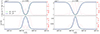 |
Fig. 8. Same as Fig. 5, but for the Sr I 4607 Å line. |
| In the text | |
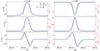 |
Fig. 9. Same as Fig. 6, but for the Sr I 4607 Å line. |
| In the text | |
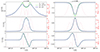 |
Fig. 10. Same as Fig. 9, but for B = 50 G. |
| In the text | |
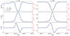 |
Fig. 11. Same as Fig. 9, but for B = 100 G. |
| In the text | |
|
Fig. 12. Same as Fig. 9, but for μ = 0.83. In this Q/I profile, we observed the maximal error between RIII and RIII−CRD calculations. |
| In the text | |
|
Fig. 13. Same as Fig. 8, but in the presence of a uniform micro-structured isotropic magnetic field with B = 20 G. |
| In the text | |
|
Fig. 14. Physical quantities of the considered 1D atmospheric model extracted from the 3D MHD Bifrost simulation en024048_hion (snapshot 385, column 120 × 120). Upper panel: strength (blue solid line), inclination (gray dashed line), and azimuth (light-blue dashed-dotted line) of the magnetic field as a function of height. Lower panel: vertical component of bulk velocity (green solid line) and temperature (red solid line) as a function of height. We adopt the convention that the velocity is positive if pointing outward in the atmosphere and negative if pointing inward. For clarity, the horizontal green dotted line indicates zero velocity. |
| In the text | |
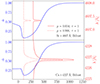 |
Fig. 15. Same as Fig. 4, but for the Bifrost atmospheric model. |
| In the text | |
|
Fig. 16. Emergent Stokes profiles for the Ca I 4227 Å line calculated in the Bifrost model (see Sect. 7), which includes height-dependent magnetic and (vertical) bulk velocity fields. The vertical gray lines show the line-center wavelength in the absence of bulk velocities. |
| In the text | |
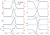 |
Fig. 17. Same as Fig. 16, but for the Sr I 4607 Å line. |
| In the text | |
Current usage metrics show cumulative count of Article Views (full-text article views including HTML views, PDF and ePub downloads, according to the available data) and Abstracts Views on Vision4Press platform.
Data correspond to usage on the plateform after 2015. The current usage metrics is available 48-96 hours after online publication and is updated daily on week days.
Initial download of the metrics may take a while.