© F. Paletou and C. Peymirat 2021

1. Introduction

The “standard” nonlocal thermodynamic equilibrium (NLTE) radiation transfer problem considers that the distribution of photons in a given “atmosphere”, that is, more generally, whatever sample of celestial body material where light–matter interactions are taking place, may depart from the equilibrium distribution described by the Planck law (Planck 1900).

It is a routinely solved problem in astrophysics which, after about six decades of constant endeavor, nowadays also considers both complex atomic models and atmospheric structures (see e.g., the monograph of Hubeny & Mihalas 2014). However, the vast majority of these problems still rely on what became a somewhat implicit assumption that the distribution of atoms both responsible for, and experiencing light–matter interactions, remain a priori known and characterized by the Maxwell–Boltzmann equilibrium distribution. Another issue related to the standard NLTE radiation transfer problem concerns the redistribution of photons after scattering onto these very massive particles, at least in frequencies if we restrict ourselves to isotropic scattering. It is also important to realize that, in the vast majority of the cases, and even though the problem of partial frequency redistribution (hereafter PRD) has been addressed quite early in the 1960s (e.g., Avrett & Hummer 1965; Auer 1968 for pioneering works), the standard NLTE problem also remains limited to the frame of complete redistribution (CRD) in most cases.

The solution of a full(er) NLTE radiation transfer problem would consist in assuming that the velocity distribution functions (VDF) of massive particles may also depart from an equilibrium distribution, as it is now commonly assumed for the photons. Therefore the solution to this problem would consist in the self–consistent resolution of a set of kinetic equations both for massive particles, potentially including free electrons, and the photons.

This general issue has already been discussed and summarized, mainly by Oxenius (1986; see also Oxenius & Simonneau 1994). However, so far and because of the inherent difficulty of the problem, only a few studies have already been conducted in the past (see e.g., Borsenberger et al. 1986, 1987).

We believe that the last decades of evolution of numerical methods (see e.g., Lambert et al. 2016 and references therein, as well as Noebauer & Sim 2019 for a recent review on Monte–Carlo radiative transfer) for radiation transfer should allow one to reconsider this issue, and evaluate up to which level of difficulty one could reasonably be able to achieve nowadays. This new evaluation should also give us new hints about which kind of astrophysical problems should be revisited, using full NLTE.

In this study, we set again the various equations governing this problem, using standard notations as much as possible. We also adopt several physical assumptions, which have already been discussed in past studies, in order to be able to set up initial numerical experiments. We discuss partial versus complete frequency redistribution, as seen from this description of the problem. We do indeed present some effects expected on departures of the VDF of excited atoms versus the Maxwell–Boltzmann distribution, as well as significative differences between computed and radiation-dependent emission profiles, and an a priori given absorption profile for a simple two-level atom model. We finally discuss future work in that somewhat forgotten physical frame for the unpolarized radiation transfer problem.

2. A simplified Boltzmann equation for massive particles

We write the evolution equation for a general distribution F(t, r, v) as follows:

$$\begin{array}{c}\hfill L[F]=C[F],\end{array}$$(1)

where L is the Liouville operator and C is the collision operator.

Therefore, the left-hand side of Eq. (1) has the general expression:

$$\begin{array}{c}\hfill L[F]=\frac{\partial F}{\partial t}+\frac{p}{m}\frac{\partial F}{\partial r}+K\frac{\partial F}{\partial p},\end{array}$$(2)

where after the time evolution term, we find an advection one and finally a force term, where we used K to avoid any confusion with the distribution F.

The right-hand side of Eq. (1) describes the various origins of collisions, which may induce modifications to the distribution. It is usually expressed as the sum of three contributions as follows:

$$\begin{array}{c}\hfill C[F]={\left(\frac{\delta F}{\delta t}\right)}_{\mathrm{rad}.}+{\left(\frac{\delta F}{\delta t}\right)}_{\mathrm{inel}.}+{\left(\frac{\delta F}{\delta t}\right)}_{\mathrm{el}.}.\end{array}$$(3)

As a matter of fact, two main mechanisms are able to produce changes in a distribution F. One of them is the so-called streaming of the massive particles, which move on their trajectories, and a second one is due to collisions between particles.

In the frame of this kinetic description, and even though the classical and academic “two-level atom” case is the simplest one we may consider, the general problem would consist in the self-consistent solution of four coupled kinetic equations for the atoms in their ground state (F₁), the atoms in their excited state (F₂), electrons (F_e), and finally the photons (I), respectively.

However, and in order to be able to make the first steps in resolving the extremely complex and cumbersome full NLTE radiation transfer problem, we shall proceed with several simplifying assumptions. First, we shall consider that only the VDF of excited atoms, that is to say F₂, may depart from a Maxwell-Boltzmann distribution. As previously discussed by Oxenius (1979), we shall consider that the velocity distribution of the ground-state atoms and the free electrons remain Maxwellian with the same temperature T. The latter is also supposed to be low enough, that is kT ≪ hν₀, where ν₀ is the central frequency of the transition between the two atomic levels of our model, so that: (i) the number density of excited atoms is much smaller than the one of ground-state atoms, that is n₂ ≪ n₁, and (ii) stimulated emission may be further neglected.

Then we shall consider a time-independent problem for photons as well as a stationary and force-free problem for atoms. And finally, following the debate between Oxenius (1965, 1979) and Hubený (1981), we shall also neglect the potential streaming (i.e., v.∂_r ≡ 0) of these excited atoms. In that frame, the Boltzmann equation for atoms can be summarized as follows:

$$\begin{array}{c}\hfill C[F_2]=0,\end{array}$$(4)

where C is the collision operator.

3. The kinetic equation of excited atoms

Each of the three contributions to the collision operator can be explained now, following Oxenius (1986).

The first one involves the radiation field and can be expressed as:

$$\begin{array}{c}\hfill {\left(\frac{\delta F_2}{\delta t}\right)}_{\mathrm{rad}.}=n_1{B}_{12}{J}_{12}(\mathit{v})f_1(\mathit{v})-n_2{A}_{21}{f}_2(\mathit{v}),\end{array}$$(5)

where stimulated emission has been neglected, and A₂₁ and B₁₂ are the usual Einstein coefficients for spontaneous emission and radiative absorption, respectively. Here, we also introduced the normalized to unity f_i distribution, such as F_i(v) = n_if_i(v).

The second one involves inelastic collisions and can be written as follows:

$$\begin{array}{c}\hfill {\left(\frac{\delta F_2}{\delta t}\right)}_{\mathrm{inel}.}=n_1{n}_e{C}_{12}{f}_1(\mathit{v})-n_2{n}_e{C}_{21}{f}_2(\mathit{v}),\end{array}$$(6)

where the C_ij are collisional (de)excitation coefficients and n_e is the electron density. We note that one may also consider that the electrons are not necessarily characterized by a Maxwell–Boltzmann velocity distribution.

Finally, and according to Oxenius (1986; see also Bhatnagar et al. 1954), a good approximation for the elastic collision term is:

$$\begin{array}{c}\hfill {\left(\frac{\delta F_2}{\delta t}\right)}_{\mathrm{el}.}=n_2{Q}_2[f^{\mathrm{M}}(\mathit{v})-f_2(\mathit{v})],\end{array}$$(7)

where Q₂ is a velocity-changing elastic collision rate. After Borsenberger et al. (1986), one may consider Q₂ = n₁v_th.σ_el., where v_th. is the “most probable” velocity of the atoms, and σ_el. is an “average cross section” for this class of elastic collision.

The scattering integral J₁₂, which appears in Eq. (5), is defined as:

$$\begin{array}{c}\hfill J_{12}(\mathit{v})={\displaystyle \oint }\frac{\mathrm{d}\mathrm{\Omega }}{4\pi }{\displaystyle \int }{\alpha }_{12}(\xi )I_{\nu }(z,\mathbf{\Omega })\mathrm{d}\nu ,\end{array}$$(8)

where α₁₂ is the atomic absorption profile and I_ν(z, Ω) is the usual specific intensity. At this stage we omit the potentiel dependence with depth z of J₁₂ on purpose, since we shall stay away from the frame of radiation transfer in this study. The specific intensity (see Sect. 4) is also dependent on the direction Ω of the radiation. All integrals dΩ mean an angular integration over all possible directions of propagation of light, as is usual in the field of radiation transfer. It is more important now to keep in mind that this scattering integral is a function of the velocity of the massive particles. Indeed, we have to take into account the Fizeau–Doppler relationship between frequency ξ in the atomic frame, and ν in the observer’s frame:

$$\begin{array}{c}\hfill \nu =\xi +\left(\frac{{\nu }_0}{c}\right)\mathit{v}·\mathbf{\Omega },\end{array}$$(9)

where v is the velocity of the atoms and Ω is the direction of propagation of the photons. This latter coupling and the explicit dependence of J₁₂ on the velocity of these “scattering centers,” which constitute the atoms present in the atmospheric plasma, also naturally lead to the role that will be played by their velocity distribution.

The atomic absorption profile α₁₂ is known a priori, and we may consider either coherent scattering, that is:

$$\begin{array}{c}\hfill {\alpha }_{12}(\xi )=\delta (\xi -{\nu }_0),\end{array}$$(10)

where ξ is the incoming photon frequency, or radiation damping which is characterized by a Lorentzian profile such that:

$$\begin{array}{c}\hfill {\alpha }_{12}(\xi )=\left(\frac{a}{\pi }\right)\frac{1}{{(\xi -{\nu }_0)}^2+a^2},\end{array}$$(11)

and where, in both cases, ν₀ is the central wavelength of the transition we consider. In the remainder of this study, we shall assume coherent scattering in the atomic frame, together with “infinitely sharp” energy levels for the model spectral line at ν₀.

It is finally important to keep in mind that at this stage the atomic emission profile η₂₁ may differ from α₁₂, in general. This, combined with possible deviations from a Maxwell–Boltzmann VDF for excited atoms will “naturally” lead to nonstandard as well as radiation-dependent redistribution in frequency for the photons.

4. The kinetic equation of the photons

The radiation transfer equation (RTE) is also the kinetic equation governing the distribution, or specific intensity I, of the photons. The correspondance between these two “forms” is nicely described in Sect. 3 of Oxenius (1986).

Assuming the very usual 1D plane–parallel geometry, the time-independent RTE can be written¹ as:

$$\begin{array}{c}\hfill \frac{\partial I_{\nu }(z,\mathbf{\Omega })}{\mathit{dz}}={\kappa }_{\nu }(z,\mathbf{\Omega })[S_{\nu }(z,\mathbf{\Omega })-I_{\nu }(z,\mathbf{\Omega })],\end{array}$$(12)

where κ_ν(z, Ω) is the absorption coefficient and S_ν(z, Ω) is the so-called source function, which a priori depends on depth z in the atmosphere, frequency ν, and direction Ω.

The absorption coefficient is usually defined as:

$$\begin{array}{c}\hfill {\kappa }_{\nu }(z,\mathbf{\Omega })=\left(\frac{h{\nu }_0}{4\pi }\right)[n_1{B}_{12}{\phi }_{\nu }(\mathbf{\Omega })-n_2{B}_{21}{\psi }_{\nu }(\mathbf{\Omega })],\end{array}$$(13)

where B₂₁ is the Einstein coefficient for stimulated emission, such as g₁B₁₂ = g₂B₂₁ assuming that the statistical weights g_i and the (line) source function is, by definition, the ratio between the emissivity:

$$\begin{array}{c}\hfill {\eta }_{\nu }(z,\mathbf{\Omega })=\left(\frac{h{\nu }_0}{4\pi }\right)n_2{A}_{21}{\psi }_{\nu }(\mathbf{\Omega }),\end{array}$$(14)

and the absorption coefficient. And finally, the more usual RTE introduces the optical depth τ_ν(Ω) = − κ_ν(z, Ω)dz in order to substitute the geometrical length for another quantity more relevant to what photons effectively experience during multiple light–matter interactions.

Should we completely neglect stimulated emission, that is to say going beyond the (very usually) adopted so-called “weak radiation field regime” for which stimulated emission is treated as “negative” absorption (as in Eq. (13)), then the source function can be simply written as:

$$\begin{array}{c}\hfill S_{\nu }(z,\mathbf{\Omega })=\frac{n_2{A}_{21}{\psi }_{\nu }(\mathbf{\Omega })}{n_1{B}_{12}{\phi }_{\nu }(\mathbf{\Omega })}.\end{array}$$(15)

This assumption is also consistent with the low–temperature assumption, which is also compatible with n₁ ≫ n₂.

Furthermore, the respective (and potentially also depth-dependent) emission and absorption profiles are defined as

$$\begin{array}{c}\hfill {\phi }_{\nu }(\mathbf{\Omega })={\displaystyle \int }{\alpha }_{12}(\xi )f_1(\mathit{v}){\mathrm{d}}^3\mathit{v}\end{array}$$(16)

and

$$\begin{array}{c}\hfill {\psi }_{\nu }(\mathbf{\Omega })={\displaystyle \int }{\eta }_{21}(\xi ,\mathbf{\Omega })f_2(\mathit{v}){\mathrm{d}}^3\mathit{v}.\end{array}$$(17)

In the latter expressions appear explicitly the respective VDFs for these atoms on the ground state, f₁, and for the ones in their first excited state, f₂.

In general, atomic profiles η₂₁ and α₁₂ are not identical. Moreover, the emission profile η₂₁ depends on the radiation field. We return to this issue in Sect. 8.

5. A two–distribution, two-level atom problem

Hereafter, we shall therefore simplify the problem, considering that only f₂ and the specific intensity I may depart from equilibrium distributions.

We shall first reassess earlier results which may still be quite largely unknown to the astronomical community by considering coherent scattering, that is α₁₂(ξ) = δ(ξ − ν₀), where ν₀ is the central wavelength of the spectral line associated with our two-level atom.

We therefore start with the additional simplifications of a stationary, force-free, and no advection (or streaming) case for which

$$\begin{array}{c}\hfill {\left(\frac{\delta F_2}{\delta t}\right)}_{\mathrm{rad}.}+{\left(\frac{\delta F_2}{\delta t}\right)}_{\mathrm{inel}.}+{\left(\frac{\delta F_2}{\delta t}\right)}_{\mathrm{el}.}=0.\end{array}$$(18)

Under these assumptions, we can derive the following expression for f₂ and, while adopting a Maxwellian velocity distribution for electrons, using the more classic formalism such that C_ij ← n_eC_ij (see also Eq. (9.51) of Hubeny & Mihalas 2014 for instance), we have

$$\begin{array}{cc}& n_2(A_{21}+C_{21})f_2(\mathit{v})+n_2{Q}_2[f_2(\mathit{v})-f^M(\mathit{v})]\hfill \\ \hfill & =n_1(B_{12}{J}_{12}(\mathit{v})+C_{12})f_1(\mathit{v}).\hfill \end{array}$$(19)

Should we assume that f_1, 2 are both Maxwellian, which is a common assumption even for NLTE radiation transfer problems, and should we integrate Eq. (19) over all velocities, we recover the classic form of the equation of statistical equilibrium (ESE) for a two-level atom case, neglecting stimulated emission:

$$\begin{array}{c}\hfill n_2(A_{21}+C_{21})=n_1(B_{12}{\displaystyle {\int }_{\mathit{v}}}{J}_{12}(\mathit{v})f^M(\mathit{v}){\mathrm{d}}^3\mathit{v}+C_{12}).\end{array}$$(20)

We shall come back to the integral term after Eq. (30). We note here that because this particular contribution vanishes after integration over velocities, the potential effects of velocity-changing elastic collisions can be considered explicitly and reasonably discussed, although only by using such a kinetic description.

Now from Eq. (19), we are able to derive an explicit expression for the nonequilibrium VDF f₂, assuming that all atoms in their fundamental state of energy follow a Maxwellian VDF, that is to say f₁ ≡ f^M. As in Borsenberger et al. (1986), we shall normalize the specific intensity to the “low temperature limit” of the Planck function, that is the Wien function:

$$\begin{array}{c}\hfill {\mathcal{B}}_W=\left(\frac{2h{\nu }_0^3}{c^2}\right)e^{-h{\nu }_0/kT}.\end{array}$$(21)

The use of this expression, instead of the Planck function, is also consistent with our assumption of a negligible rate of stimulated emission. We shall also define the ratio

$$\begin{array}{c}\hfill {\overline{J}}_{12}=J_{12}/{\mathcal{B}}_W\end{array}$$(22)

as well as use the following relationships, first between Einstein coefficients

$$\begin{array}{c}\hfill \frac{A_{21}}{B_{21}}=\left(\frac{2h{\nu }_0^3}{c^2}\right),\end{array}$$(23)

with g₁B₁₂ = g₂B₂₁, and where g_1, 2 are the statistical weights of each level.

In addition, collisional rates are such that

$$\begin{array}{c}\hfill n_1^{\ast }{C}_{12}=n_2^{\ast }{C}_{21},\end{array}$$(24)

where $n_{1,2}^{*}$ are the LTE values of the respective densities of population, satisfying the Boltzmann law:

$$\begin{array}{c}\hfill \left(\frac{n_2^{\ast }}{n_1^{\ast }}\right)=\left(\frac{g_2}{g_1}\right)e^{-h{\nu }_0/kT}.\end{array}$$(25)

We shall therefore now introduce the normalized population, which allows for some measurement of deviations from LTE: ${\overline{n}}_2=n_2/n_2^{\ast }$.

We now introduce:

$$\begin{array}{c}\hfill \epsilon =\frac{C_{21}}{A_{21}+C_{21}},\end{array}$$(26)

which is another parameter otherwise traducing the amount of “departure from LTE” in a given atmosphere, and the less common:

$$\begin{array}{c}\hfill \zeta =\frac{Q_2}{A_{21}+C_{21}},\end{array}$$(27)

which characterizes the amount of elastic collisions. Assuming that $n_1=n_1^{*}$ and f₁ ≡ f^M, we may now rewrite the following:

$$\begin{array}{c}\hfill {\overline{n}}_2{f}_2(\mathit{v})-{\overline{n}}_2\zeta [f^M(\mathit{v})-f_2(\mathit{v})]=[\epsilon +(1-\epsilon ){\overline{J}}_{12}(\mathit{v})]f^M(\mathit{v}).\end{array}$$(28)

This expression is indeed identical to Eq. (2.44) of Borsenberger et al. (1986) when one neglects streaming of particles (his η = 0).

Now, integrating Eq. (28) over all velocities, we find that:

$$\begin{array}{c}\hfill {\overline{n}}_2=\epsilon +(1-\epsilon ){\mathcal{J}}_{12},\end{array}$$(29)

where we defined

$$\begin{array}{c}\hfill {\mathcal{J}}_{12}={\displaystyle {\int }_{\mathit{v}}}{\overline{J}}_{12}(\mathit{v})f^M(\mathit{v}){\mathrm{d}}^3\mathit{v},\end{array}$$(30)

which is equivalent to the common $\overline{J}$ scattering integral used in the standard approach. We finally recover the following:

$$\begin{array}{c}\hfill f_2(\mathit{v})=[\frac{\zeta }{1+\zeta }+\left(\frac{1}{1+\zeta }\right)\frac{\epsilon +(1-\epsilon ){\overline{J}}_{12}(\mathit{v})}{\epsilon +(1-\epsilon ){\mathcal{J}}_{12}}]f^M(\mathit{v}).\end{array}$$(31)

This is the central relationship allowing us to quantify departures from “Maxwellianity” for f₂ and potential differences between macroscopic emission and absorption profiles, depending on the nature of the radiation field characterized by I.

6. Two comments on the standard theory

Complete redistribution in frequency relies on the a priori assumption that the “macroscopic” emission and absorption profile are identical. Then the line source function reduces to the simple ratio S = n₂A₂₁/n₁B₁₂, that is to say a quantity independent of the frequency after Eq. (15). It is also a considerable simplification of the NLTE radiation transfer problem. Assuming, as we do here, that the atomic profiles are identical, that is, α₁₂ ≡ η₂₁, CRD also assumes the identity implicitly as follows:

$$\begin{array}{c}\hfill f_2\equiv f_1(\equiv f^M),\end{array}$$(32)

whose effects therefore result from expressions given in Eqs. (16) and (17). In that frame, we also recover that the normalized source function $\overline{S}=S/B_W$ is such that

$$\begin{array}{c}\hfill \overline{S}={\overline{n}}_2=\epsilon +(1-\epsilon ){\mathcal{J}}_{12}.\end{array}$$(33)

This expression is indeed consistent with the classical (CRD) “two-level atom” case described in any radiation transfer textbook following the publication of Avrett & Hummer (1965).

However, in eliminating the case of little astrophysical interest of an isotropic “white” radiation field, Eq. (32) is clearly inconsistent with the more general Eq. (31), unless setting ζ = 0 and ε = 1, that is assuming LTE. Therefore NLTE should always come together with some partial frequency redistribution and no complete redistribution a priori.

Additionally, even when “standard” partial frequency redistribution is used, with a priori known redistribution functions, in most cases a “branching ratio” usually defined as

$$\begin{array}{c}\hfill \gamma =\frac{A_{21}+C_{21}}{A_{21}+C_{21}+Q_E}\end{array}$$(34)

is introduced (see Omont et al. 1972; Heinzel & Hubený 1982; Heinzel et al. 1987) to form a linear combination of R_II and R_III redistribution such as

$$\begin{array}{c}\hfill R(x^{\prime },x)=\gamma R_{\mathrm{II}}(x^{\prime },x)+(1-\gamma )R_{\mathrm{III}}(x^{\prime },x),\end{array}$$(35)

following the nomenclature of Hummer (1962), and where x′ and x are the usual incoming and outgoing reduced frequencies, respectively, which are usually defined as:

$$\begin{array}{c}\hfill x=\frac{\nu -{\nu }_0}{\mathrm{\Delta }{\nu }_D},\end{array}$$(36)

with the Doppler width Δν_D = (ν₀/c)v_th. and the most probable velocity $v_{th.}=\sqrt{2kT/M}$ as usual.

The elastic collision rate Q_E which appears in the branching ratio γ should not be confused with the Q₂ elastic collision rate introduced in Eq. (7). The latter is indeed, and more precisely, the rate of these velocity-changing elastic collisions, that is a fraction of the total amount Q_E of elastic collisions. Bommier (2016a), for instance, provides a synthetic but accurate and valuable explanation about the different classes of elastic collisions. Moreover, as mentioned in this discussion, Landi Degl’Innocenti & Landolfi (2004; see their Sect. 13.2) estimate that Q₂ should be very small in solar–like atmospheres, so that the so-called Boltzmann elastic collision term may be practically neglected for radiative modeling under such physical conditions.

Nevertheless, quantifying any significant effet due to elastic collisions in the NLTE problem for other atmospheres with physical conditions characterized by a more important amount of velocity-changing collisions than in the solar–like case would thus require using the more general theoretical frame we adopt here (see also Belluzzi et al. 2013 for instance). Indeed, using velocity integrated expressions such as Eqs. (20) or (29), which is the case in the standard NLTE approach, and even with standard PRD, the elastic collision term introduced in Eq. (7) just vanishes.

7. Quantifying departures from equilibrium

The stage is now set for the first evaluation of potential departures from “Maxwellianity,” owing to the nature of the radiation field we may adopt.

For a first exploration, we shall first assume pure Doppler broadening for the spectral line, that is to say coherent scattering in the atom’s frame and

$$\begin{array}{c}\hfill {\alpha }_{12}(\xi )={\eta }_{21}(\xi )=\delta (\xi -{\nu }_0),\end{array}$$(37)

where both atomic profiles are also assumed to be isotropic. Should we moreover assume no elastic collisions so far, that is ζ = 0, then after Eq. (31) we end up with

$$\begin{array}{c}\hfill f_2(\mathit{u})=\left[\frac{\epsilon +(1-\epsilon ){\overline{J}}_{12}(\mathit{u})}{\epsilon +(1-\epsilon ){\mathcal{J}}_{12}}\right]f^M(\mathit{u}),\end{array}$$(38)

where we also introduced the normalized velocity u = v/v_th..

NLTE implies that ε < 1, which in turn necessarily implies that f₂ differs from being Maxwellian in general. Should these differences be significant enough, then after Eq. (17) and despite the equality between respective atomic profiles, we however expect differences between macroscopic absorption and emission profiles, unlike what assumes, ab initio, the widely adopted CRD.

The abovementioned assumptions lead to

$$\begin{array}{c}\hfill {\overline{J}}_{12}(u)=\frac{1}{2u}{\displaystyle {\int }_{-u}^{+u}I(x)\mathrm{d}x.}\end{array}$$(39)

Then, since f₁ ≡ f^M, using this classical expression for the (normalized to unity) macroscopic absorption profile

$$\begin{array}{c}\hfill {\phi }_x=\frac{1}{\sqrt{\pi }}{e}^{-x^2},\end{array}$$(40)

we can also establish that

$$\begin{array}{c}\hfill {\mathcal{J}}_{12}=\frac{1}{\sqrt{\pi }}{\displaystyle {\int }_{-\infty }^{+\infty }I(x)e^{-x^2}\mathrm{d}x,}\end{array}$$(41)

which finally allows us to evaluate departures of f₂ from the equilibrium distribution depending on the thus far given (and normalized to unity) radiation field I(x).

According to these expressions, one can notice that, with coherent scattering in the atom’s frame, it remains however an ultimate option for “saving” the CRD case. Indeed, assuming isotropic “white” light illumination, that is a frequency independent radiation field such as I(x) = I₀, is the only condition left to us in order to keep f₂ ≡ f^M and therefore ψ_x ≡ φ_x.

Further illustrative computations have been made using several incident radiation profiles, as displayed in Fig. 1. Our selection covers distinct possibilities of central reversal amplitudes, that is to say I_max./I(0) as well as peaks located at different and increasing positions away from line center. These may mimic some observed and well-resolved resonance line profiles, similar to one of the good candidates for future modeling such as Lyα of H I.

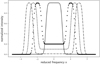Fig. 1. Isotropic and normalized intensity profiles I vs. the reduced frequency x, used for the evaluation of departures from the equilibrium velocity distribution for the VDF of these excited atoms, f2. We adopted different values for (i) the location of the (symmetric) peaks, and (ii) of the central reversal of each profile. These variations can also mimic some resonance lines observations that may form under different astrophysical conditions.

Then, we computed ratios of f₂/f^M according to Eq. (38), and further adopting ε = 0. Our results for f₂/f^M as a function of the normalized velocity u are displayed in Fig. 2, for which we used the same linestyle convention as in Fig. 1.

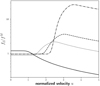Fig. 2. Ratios f2/fM as a function of the normalized velocity u, for different radiation field profiles, and for ε = 0 and ζ = 0. The same linestyle convention as in Fig. 1 was adopted. The magnitude of these departures from a Maxwellian velocity distribution depends on both (i) the distance of the peaks of I vs. line center, and (ii) the amount of its central reversal characterized by Imax./I(0).

Departures from a Maxwellian distribution show up at almost all normalized velocities u. These departures tend to increase both with (i) an increasing distance of the peaks of the incident radiation profile away from line center, as well as with (ii) an increase of the central reversal of the incident profile, which is characterized by the ratio between the maximum value of the profile I_max and its central value I(0).

Finally, it is also possible to compute the ratio between the macroscopic emission profile ψ_x and the (Gaussian) absorption profile φ_x. Indeed, after Eqs. (38) and (17), and with ε = 0, one can derive (see also Appendix A) that

$$\begin{array}{c}\hfill {\psi }_x=\frac{2}{\sqrt{\pi }{\mathcal{J}}_{12}}{\displaystyle {\int }_{|x|}^{\infty }{\overline{J}}_{12}(u)u{e}^{-u^2}\mathrm{d}u,}\end{array}$$(42)

for the case of coherent scattering in the atom’s frame.

We also note that, at this stage, with the knowledge of the radiation-dependent emission profile, we are also able to compute the source function, following Eq. (15).

Significant differences between emission and absorption profiles are put in evidence from our relatively simple computations. They are displayed in Fig. 3 which shows macrocopic profile ratios as a function of x for the same set of incident radiation profiles as before.

Fig. 3. Ratios ψx/φx as a function of the reduced frequency x, for the different radiation field profiles displayed in Fig. 1, using also the same linestyle convention. We observe here, for the case of coherent scattering in the atom’s frame, similar tendencies as the ones displayed in Fig. 2 for the ratios between VDFs.

For these ratios and the special case of coherent scattering in the atom’s frame, we observe the same tendancies as the ones already observed for the ratio between VDFs. It essentially shows the very limit of the theoretical framework of CRD and its intrinsic inconsistency with NLTE.

8. Discussion

So far, the radiation field has been imposed a priori using a simple I(x) function. Potential anisotropies of the radiation field could be taken into account within this formalism of course. Also, more realistic line profiles will be adopted further, as we did for the computation of the ratio f₂/f^M displayed in Fig. 4. In that case, we used the profile of the H I Lyα resonance line deduced from SoHO/Sumer solar observations (Gunár et al. 2020, in particular their Fig. 5). We adopted a temperature of 10⁴ K, leading to a I(x) profile extending up to x ∼ 30. Then we fixed ζ = 0 and ε = 10⁻⁷, that is a value which is quite typical of conditions usually met in solar prominences for instance (see e.g., Paletou et al. 1993). Departures from a Maxwellian distribution mainly appear significant around the peak of the line profile at x ∼ 5 in our case, and in the line wings.

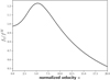Fig. 4. Ratio f2/fM vs. the normalized velocity u for ε = 10−7 (ζ = 0), and a realistic H I Lyα illumination profile as observed by SoHO/Sumer. The peak of the line profile is located at x ∼ 5, and the central self-reversal is about 0.7 for this resonance line (see Fig. 5 of Gunár et al. 2020).

But the most important thing to address further will be the self–consistent computation of the two distributions f₂ and I. This should be possible within an iterative cycle involving the following: an initial guess for the source function S assuming for instance both LTE and CRD, then a formal solution for the RTE, allowing for the computation of ${\overline{J}}_{12}$ and 𝒥₁₂. Then f₂ should be estimated, as well as ψ_x, making it possible to update the source function further, start another iteration, and so forth, until reaching convergence for both f₂ and I.

We believe that state-of-the-art iterative methods presently used for NLTE radiative transfer (see e.g., Lambert et al. 2016, and references therein) will allow one to explore all of the potential of this alternative and a more detailed theoretical frame, beyond what could be achieved at that time by Borsenberger et al. (1986, 1987) and Atanackovič et al. (1987).

In parallel with this numerical set-up, we shall also consider the more realistic case of “natural broadening” of the upper level of the atomic transition. The alternative atomic absorption profile is now a Lorentzian profile, whose expression was given in Eq. (11). However, in such a case, atomic absorption and emission profiles will be different since the atomic emission profile will now depend explicitly on the radiation field. Expressions for this emission profile η₂₁ are discussed in Appendix B of Oxenius (1986); see also Hubený et al. (1983; their Sect. 4.3). The derivation of the latter expressions remains, however, questionable and it more likely leads to erroneous coefficients (V. Bommier, priv. comm.). Therefore, the modified emissivity consisting in the sum of a “classical” (order-2) term with an extra “order-4” contribution proposed by Bommier (1997) will be preferred. In that frame, based on sound physical grounds, it appears that only the order-2 term emissivity will be associated with the iterative modifications of the VDF of the excited atoms. Indeed, the so-called order-4 coefficient introduced by Bommier (1997) involves the lower level atomic state (see her Eq. (92) for the unpolarized case). However, as well as the order-2 contribution (via the statistical equilibrium equation), the order-4 contribution² to emissivity depends on the radiation field, so that will also be need in order to be “runned to convergence” together with the distributions I and f₂. The associated numerical burden will mainly amount to recomputing Voigt-like functions (see e.g., Paletou et al. 2020) at every iteration, according to changes in f₂ and I, and at every depth in the atmosphere.

Finally, any significant effect of these velocity-changing elastic collisions, which are “by construction” not taken into account in the standard NLTE approach, could be properly discussed for different astrophysical situations using the present formalism.

9. Conclusion

We have revisited and rewritten basic elements of Oxenius’ kinetic approach for NLTE spectral line formation, using more conventional notations for. We also brought clarification to some technical parts which were not always clearly explained in his textbook and some other subsequent, but still remaining “little acknowledged” studies. We note that similar elements of this approach have been recently discussed again in the more complete, but more likely less accessible frame of polarized radiation transfer, using the density matrix formalism (see e.g., Belluzzi et al. 2013).

Here we fully agree with the statement about “the necessity of resolving the statistical equilibrium equations for each velocity class” expressed by Bommier (2016b; see her Sect. 5.3). Therefore, in a next step, we shall implement an iterative numerical scheme, based on pre-existing practices in astrophysical radiation transfer (see e.g., Lambert et al. 2016 and references therein) in order to compute self–consistently both for the specific intensity (or distribution of the photons) and, in a first stage, for the velocity distribution of these excited atoms present in the atmosphere. As a matter of fact, directly tackling the computation of the VDF of excited atoms also naturally leads to a generalization of the PRD theoretical frame, somewhat, without using any a priori defined redistribution function.

This will allow us to identify further and explore in more detail plausible astrophysical situations for which this “full–NLTE” approach for the very general issue of spectral line formation will prove to be indispensable.

Acknowledgments

We are grateful to Dr Stanislav Gunár (Astronomical Institute of the Czech Academy of Sciences) who very kindly made his data available to us. We also thank an anonymous referee, and Dr Véronique Bommier (Cnrs and Observatoire de Paris, France) for valuable comments and encouragement. Finally Frédéric Paletou is grateful to his radiative transfer Sensei, Dr. L. H. “Larry” Auer, with whom we started discussing about these issues long time ago.

References

Appendix A: Derivation of the macroscopic emission profile ψ_x

We find it quite unfortunate that in his monograph, Oxenius (1986) did not make the derivation of the macroscopic emission profile, whose expression is given in Eq. (42), explicit. This is why we propose the following steps.

We shall first assume that

$$\begin{array}{c}\hfill {\displaystyle \oint }\delta (x-\mathit{u}·\mathbf{\Omega })\mathrm{d}\mathrm{\Omega }=\frac{2\pi }{u}H(u-|x|),\end{array}$$(A.1)

where H is the usual Heaviside or unit step function. Using such an angular integration for the combination of our Eqs. (17) and (38) when ε = 0 can be written as follows:

$$\begin{array}{c}\hfill {\psi }_x=\frac{1}{{\mathcal{J}}_{12}}{\displaystyle \oint }(\int {\overline{J}}_{12}(\mathit{u})\delta (x-\mathit{u}·\mathbf{\Omega })f^M(\mathit{u}){\mathrm{d}}^3\mathit{u})\frac{\mathrm{d}\mathrm{\Omega }}{4\pi }.\end{array}$$(A.2)

First, the angular integration will transform the Dirac distribution modeling coherent scattering, into the Heaviside function.

Then, using spherical coordinates in the velocity space for the integration in u, that is

$$\begin{array}{c}\hfill {\mathrm{d}}^3\mathit{u}=u^{2}sin(\theta )\mathrm{d}u\mathrm{d}\theta \mathrm{d}\phi ,\end{array}$$(A.3)

where θ and φ are the usual, respectively, polar angle and azimuth, one gets

$$\begin{array}{c}\hfill {\psi }_x=\frac{2\pi }{{\pi }^{3/2}{\mathcal{J}}_{12}}{\displaystyle \int }{\overline{J}}_{12}(u)u{e}^{-u^2}H(u-|x|)\mathrm{d}u,\end{array}$$(A.4)

which finally leads to Eq. (42) using the property of the H function which is then different from 0 for u ≥ |x|.

All Figures

Fig. 1. Isotropic and normalized intensity profiles I vs. the reduced frequency x, used for the evaluation of departures from the equilibrium velocity distribution for the VDF of these excited atoms, f2. We adopted different values for (i) the location of the (symmetric) peaks, and (ii) of the central reversal of each profile. These variations can also mimic some resonance lines observations that may form under different astrophysical conditions.

In the text

Fig. 2. Ratios f2/fM as a function of the normalized velocity u, for different radiation field profiles, and for ε = 0 and ζ = 0. The same linestyle convention as in Fig. 1 was adopted. The magnitude of these departures from a Maxwellian velocity distribution depends on both (i) the distance of the peaks of I vs. line center, and (ii) the amount of its central reversal characterized by Imax./I(0).

In the text

	Fig. 3. Ratios ψx/φx as a function of the reduced frequency x, for the different radiation field profiles displayed in Fig. 1, using also the same linestyle convention. We observe here, for the case of coherent scattering in the atom’s frame, similar tendencies as the ones displayed in Fig. 2 for the ratios between VDFs.
In the text

	Fig. 4. Ratio f2/fM vs. the normalized velocity u for ε = 10−7 (ζ = 0), and a realistic H I Lyα illumination profile as observed by SoHO/Sumer. The peak of the line profile is located at x ∼ 5, and the central self-reversal is about 0.7 for this resonance line (see Fig. 5 of Gunár et al. 2020).
In the text

References

- Atanackovič, O., Borsenberger, J., Oxenius, J., & Simonneau, E. 1987, JQSRT, 38, 427 [Google Scholar]
- Auer, L. H. 1968, ApJ, 153, 783 [Google Scholar]
- Avrett, E. H., & Hummer, D. G. 1965, MNRAS, 130, 295 [Google Scholar]
- Belluzzi, L., Landi Degl’Innocenti, E., & Trujillo Bueno, J. 2013, A&A, 552, A72 [NASA ADS] [CrossRef] [EDP Sciences] [Google Scholar]
- Bhatnagar, P. L., Gross, E. P., & Krook, M. 1954, Phys. Rev., 94, 511 [Google Scholar]
- Bommier, V. 1997, A&A, 328, 706 [NASA ADS] [Google Scholar]
- Bommier, V. 2016a, A&A, 591, A59 [Google Scholar]
- Bommier, V. 2016b, A&A, 591, A60 [EDP Sciences] [Google Scholar]
- Borsenberger, J., Oxenius, J., & Simonneau, E. 1986, JQSRT, 35, 303 [Google Scholar]
- Borsenberger, J., Oxenius, J., & Simonneau, E. 1987, JQSRT, 37, 331 [Google Scholar]
- Gunár, S., Schwartz, P., Koza, J., & Heinzel, P. 2020, A&A, 644, A109 [EDP Sciences] [Google Scholar]
- Heinzel, P., & Hubený, I. 1982, JQSRT, 27, 1 [Google Scholar]
- Heinzel, P., Gouttebroze, P., & Vial, J.-C. 1987, A&A, 183, 351 [NASA ADS] [Google Scholar]
- Hubený, I. 1981, A&A, 100, 314 [Google Scholar]
- Hubeny, I., & Mihalas, D. 2014, Theory of Stellar Atmospheres (Princeton University Press) [Google Scholar]
- Hubený, I., Oxenius, J., & Simonneau, E. 1983, JQSRT, 29, 447 [Google Scholar]
- Hummer, D. G. 1962, MNRAS, 125, 21 [Google Scholar]
- Lambert, J., Paletou, F., Josselin, E., & Glorian, J.-M. 2016, Eur. J. Phys., 37, 015603 [Google Scholar]
- Landi Degl’Innocenti, E., & Landolfi, M. 2004, Polarization in Spectral Lines (Kluwer) [Google Scholar]
- Noebauer, U. M., & Sim, S. A. 2019, Liv. Rev. Comput. Astrophys., 5, 1 [Google Scholar]
- Omont, A., Smith, E. W., & Cooper, J. 1972, ApJ, 175, 185 [Google Scholar]
- Oxenius, J. 1965, JQSRT, 5, 771 [Google Scholar]
- Oxenius, J. 1979, A&A, 76, 312 [Google Scholar]
- Oxenius, J. 1986, Kinetic theory of particles and Photons - Theoretical Foundations of non-LTE Plasma Spectroscopy (Springer) [Google Scholar]
- Oxenius, J., & Simonneau, E. 1994, Ann. Phys., 234, 60 [Google Scholar]
- Paletou, F., Vial, J.-C., & Auer, L. H. 1993, A&A, 274, 571 [NASA ADS] [Google Scholar]
- Paletou, F., Peymirat, C., Anterrieu, E., & Böhm, T. 2020, A&A, 633, A111 [EDP Sciences] [Google Scholar]
- Planck, M. 1900, Verhandl. Dtsch. Phys. Ges. Berlin, 2, 237 [Google Scholar]