| Issue |
A&A
Volume 671, March 2023
|
|
|---|---|---|
| Article Number | A93 | |
| Number of page(s) | 6 | |
| Section | Astrophysical processes | |
| DOI | https://doi.org/10.1051/0004-6361/202244908 | |
| Published online | 09 March 2023 | |
Full non-LTE spectral line formation
II. Two-distribution radiation transfer with coherent scattering in the atom’s frame
1
Université de Toulouse, UPS-Observatoire Midi-Pyrénées, CNRS, CNES, IRAP, 31028 Toulouse Cedex 4, France
e-mail: This email address is being protected from spambots. You need JavaScript enabled to view it.
2
CNRS, Institut de Recherche en Astrophysique et Planétologie, 14 av. E. Belin, 31400 Toulouse, France
3
Indian Institute of Astrophysics, Koramangala, Bengaluru 560034, India
4
Université de Toulouse, Faculté des Sciences et de l’Ingénierie, 31062 Toulouse Cedex 9, France
Received:
7
September
2022
Accepted:
8
January
2023
Abstract
In this article we discuss a method for obtaining a numerical solution to the so-called full nonlocal thermodynamic equilibrium (non-LTE) radiation transfer problem. More specifically, the usual numerical iterative methods for non-LTE radiation transfer are coupled with that formalism and new numerical additions are explained in detail. We benchmarked the whole process with the standard non-LTE transfer problem for a two-level atom with Hummer’s RI − A partial frequency redistribution function. Finally, we present new quantities, such as the spatial distribution of the velocity distribution function of excited atoms, which can only be accessed by adopting a more general frame for non-LTE radiation transfer, such as the one we propose here.
Key words: radiation mechanisms: general / radiative transfer / line: profiles / methods: numerical
© The Authors 2023
 Open Access article, published by EDP Sciences, under the terms of the Creative Commons Attribution License (https://creativecommons.org/licenses/by/4.0), which permits unrestricted use, distribution, and reproduction in any medium, provided the original work is properly cited.
This article is published in open access under the Subscribe to Open model. This email address is being protected from spambots. You need JavaScript enabled to view it. to support open access publication.
1. Introduction
Oxenius (1986) formulated the so-called full nonlocal thermodynamic equilibrium (non-LTE) radiation transfer problem, wherein the distribution of photons as well as the massive particles in a stellar atmosphere may both generally deviate from their equilibrium distributions. Paletou & Peymirat (2021, hereafter PP21) revisited this formalism and reconsidered some of its basic elements using standard notations prevalent in this field of research. In PP21, however, we limited ourselves to the more detailed statistical equilibrium equations for the simplest case of a “two-distribution” model.
The present study is devoted to the coupling of that formalism with usual numerical methods used for radiation transfer. The set and sequence of the new quantities, required for our computations in the continuation and sometimes the generalization of relationships previously discussed in PP21, are outlined in Sect. 2.
The validation of these new elements, dealing directly with the coupling of the frequency dependence of the radiation and the velocities of the atoms scattering light, is first made for the case of coherent scattering “in the atom’s frame”. We can indeed show (see Sect. 3) that the latter assumption for our two-distribution problem makes it equivalent to a two-level atom problem with the standard angle-averaged partial frequency redistribution (PRD) function RI − A for isotropic scattering introduced by Hummer (1962).
Useful details about the very numerical implementation of our new computations are presented in Sect. 4 and a simple iterative scheme is described in Sect. 5. We fully rely on a typical short-characteristics formal solver, mostly used for iterative methods such as accelerated Λ-iteration (hereafter, ALI), whose material was developed and made available by us1 in Python (see e.g., Lambert et al. 2016 and references therein).
A first and indispensable validation is presented in Sect. 6 by reproducing results for standard PRD-RI − A of Hummer (1969). It is however shown that the two-distribution model provides additional physical quantities, which cannot be accessed using the classical non-LTE framework, such as the spatial distribution of the velocity distribution function (hereafter, VDF; see Sects. 6 and 8) of the excited atoms. In Sects. 7 and 8, we therefore present a preliminary exploration of the effects of velocity-changing elastic collisions and new computations for a strongly illuminated finite slab case, respectively. Finally, we discuss the various conclusions and prospects of this study.
2. Coupling to radiation transfer
The implementation of our kinetic approach together with radiation transfer first requires two major modifications of existing numerical radiation transfer tools. Following Paletou & Peymirat (2021), we adopted both the reduced frequency, x, and the normalized atomic velocity, u. The reduced frequency is usually defined in radiation transfer as x = (ν − ν0)/ΔνD that is, the frequency shift from the line center normalized to the Doppler width ΔνD = (ν0/c)vth., where c is the speed of light; while u is the modulus of the atomic velocity normalized to the “most probable velocity”,  , with k being the Boltzmann constant, T the temperature, and M the mass of the atom.
The first requirement is the computation of the scattering integral J12 defined as:
 (1)
(1)
in the case of coherent scattering in the atomic frame, where δ is the Dirac distribution for the a priori known absorption profile and I(x, Ω, τ) is the usual specific intensity. The latter is computed at every frequency, x, photon propagation direction, Ω, and optical depth, τ, using a “classic” short characteristic based formal solver (see e.g., Lambert et al. 2016, and associated resources). Once this quantity is available, our modified formal solver calls a specific function that performs the angular integration over the Dirac distribution δ(x − u ⋅ Ω), adapted from Sampoorna et al. (2011; see also Sect. 4).
In a second step, we compute  , with ℬW denoting the Planck function in the Wien limit, and:
 (2)
(2)
with fM(u) = e−u ⋅ u/π3/2 for the Maxwellian velocity distribution. Here d3u = u2dudΩu wherein dΩu = sin θudθudϕu, with θu and ϕu denoting the polar angles of the normalized atomic velocity vector u about the atmospheric normal.
Once we have computed these two quantities, we can evaluate the velocity distribution function of the first excited state of the atom2 using, as defined in PP21:
![Mathematical equation: $$ \begin{aligned} f_2(\boldsymbol{u}, \tau ) = \left[ \frac{\zeta }{1+\zeta } + \left(\frac{1}{1+\zeta }\right) \frac{\varepsilon + (1-\varepsilon ) \bar{J}_{12} (\boldsymbol{u}, \tau )}{\varepsilon + (1-\varepsilon ) {\mathcal{J} }_{12}} \right] f^{M}(\boldsymbol{u}) , \end{aligned} $$](/articles/aa/full_html/2023/03/aa44908-22/aa44908-22-eq5.gif) (3)
(3)
at every depth in the atmosphere. In this expression, ε is the usual collisional destruction probability of standard non-LTE radiation transfer. However, another quantity ζ appears now, which characterizes the amount of velocity-changing elastic collisions defined in Eq. (27) of PP21 (noting again that in PP21 the depth dependence of the different quantities such as  , f2 and so on were omitted, as radiative transfer was not considered in detail at this stage).
The next critical quantity is the computation of the emission profile, which is defined, at a given optical depth τ in our (1D) atmosphere as:
 (4)
(4)
where f2 is the VDF of the excited atoms scattering light, computed using Eq. (3). At this stage, we apply Eq. (A.1) of PP21 to first perform the integral over dΩ and then perform the integral over dΩu to give:
![Mathematical equation: $$ \begin{aligned} \psi (x, \tau ) = \frac{2}{\sqrt{\pi }} \int _{|x |}^{\infty }{ \left[ \frac{\zeta }{1+\zeta } + \left(\frac{1}{1+\zeta }\right) \frac{\varepsilon + (1-\varepsilon ) \tilde{J}_{12} (u, \tau )}{\varepsilon + (1-\varepsilon ) \mathcal{{J}}_{12}} \right] u e^{-u^2} \mathrm{d}u } , \end{aligned} $$](/articles/aa/full_html/2023/03/aa44908-22/aa44908-22-eq8.gif) (5)
(5)
where
 (6)
(6)
Clearly, the emission profile given in Eq. (5) above represents the generalization of the same analytical angular integration result in Eq. (42) of PP21, which, however, was written only for the ζ = 0 and ε = 0 cases.
Once all the quantities defined by Eqs. (1)–(5) have been evaluated, one may then compute the source function. Hereafter, we shall use the below expression (not given explicitly in PP21) for the source function:
![Mathematical equation: $$ \begin{aligned} S(x, \tau ) = \left[ \varepsilon + (1 - \varepsilon ) {\mathcal{J} }_{12}(\tau ) \right] \left[ {{\psi (x, \tau )} \over {\varphi (x)}} \right] , \end{aligned} $$](/articles/aa/full_html/2023/03/aa44908-22/aa44908-22-eq10.gif) (7)
(7)
where φ is the so-called Doppler absorption profile. It is quite straightforward to establish and this is indeed the very expression of the source function that we used in the present study (noting that this expression remains unchanged when ζ ≠ 0).
3. Equivalence with Hummer’s RI − A redistribution
It is easy to show that a “two-distribution” model assuming a Maxwellian distribution for f1, characterizing the fundamental level, and coherent scattering in the atom’s frame is equivalent to a standard PRD model for a two-level atom problem considering Hummer’s angle-averaged (and isotropic scattering) RI − A redistribution. It therefore provides a critical benchmark for our modified numerical tools.
A way to verify this equivalence is by using the developed expression of the emission profile given by the combination of Eqs. (3) and (4), together with Eq. (7). This should also be considered for ζ = 0 since this new parameter is not relevant to standard PRD using Hummer’s redistribution functions. Then, we may split in two the expression of the emission profile with a first part, which goes like εfM(u), and another one that implies  besides the common denominator which is independent from u. The first part, after integrations, will lead to the Doppler absorption profile φ, since it is the convolution of the Dirac function characterizing coherent scattering in the atom’s frame with the Maxwellian VDF fM(u). However, most interesting is however the second part involving
  . For this second part, we go back to real frequencies ξ (in the atomic frame) and ν (in the observer’s frame), from x and the Doppler transform (see also the notations adopted in PP21). Now the Dirac function appearing in Eq. (4) becomes δ(ξ − ν0), while that in Eq. (1) when substituted in Eq. (4) becomes δ(ξ′−ν0). Thus, the second part of the emission profile contains the product of two Dirac distributions, namely, δ(ξ − ν0)δ(ξ′−ν0). We can also rewrite this combination as: δ(ξ − ν0)δ(ξ′−ξ) which is indeed the atomic redistribution function rI (see e.g., Hubeny & Mihalas 2014). This has also been discussed in Sect. 4 of Borsenberger et al. (1987).
After integration over velocities along the Maxwellian VDF, and after angular integration, we finally recover the more usual form of the standard PRD, frequency-dependent source function (normalized to the Planckian):
![Mathematical equation: $$ \begin{aligned} S(x, \tau ) = \varepsilon + (1 - \varepsilon ) \oint { { {\mathrm{d}\Omega^\prime } \over {4 \pi } } } \int _{x^\prime } { \left[ \frac{R_{I-A}(x^\prime ,x)}{\varphi (x)} \right] I(x^\prime , \Omega^\prime , \tau ) \mathrm{d}x^\prime } . \end{aligned} $$](/articles/aa/full_html/2023/03/aa44908-22/aa44908-22-eq13.gif) (8)
(8)
The solution of such a problem can easily be computed using the methods proposed by Paletou & Auer (1995).
4. Numerical implementation
Our numerical implementation of the new, full non-LTE problem relies on modifications brought to a nowadays classic short-characteristics (hereafter, SC) based formal solver (see e.g., Lambert et al. 2016, and references therein). This, together with various iterative schemes which can be set on that basis constitutes a more efficient way, both fast and accurate, as well as easy to develop on, to address the problem than what was made previously by Borsenberger et al. (1986, 1987) and Atanackovič et al. (1987).
The main numerical problem now, as compared to the standard non-LTE problem, is to properly evaluate expressions given by Eqs. (1) and (4). First is the angular integration for making J12. It consists in using a quadrature in polar angle and azimuth (θ, ϕ) both for the ray direction and for the atomic velocity. Then, one may write: u ⋅ Ω = γu where:
 (9)
(9)
Here, indices r and u are respectively associated with the ray and the atomic velocity directions.
Once γ has been computed for every couple of polar angle and azimuth, the specific intensity is interpolated in x in order to estimate the I(x = γu) quantity that will contribute to the integral leading to J12(u, τ), after a first integration in frequency along the atomic absorption profile. A mere linear interpolation was used together with our identical x and u grids, hereafter, spanning 6 Doppler width in x, with Δu = Δx = 0.1. To achieve this very task, we use a dedicated function which is called in from the usual SC formal solver, once the specific intensity is available at all frequencies, at a given depth and direction.
Practically, we used a ten-point regularly spaced quadrature for ϕ in the [0, 2π] domain, together with Gauss-Legendre nodes for the direction cosines usually defined in radiation transfer as: μ = cos(θr). Most computations have used six nodes for μ, thus leading to 60 distinct couples (θ, ϕ). We also note that our new formal solver was designed for considering full frequency and angular dependence of the source function.
The numerical calculation of 𝒥12 is straightforward. Here, for the integration over dΩu we use the same angular quadrature as mentioned above. The integration over the modulus of the atomic velocity u can be done either using a simple trapezoidal rule or a Gauss-Hermite quadrature.
Then follows another similar numerical integration over atomic velocities, leading to the self-consistent emission profile, according to Eq. (5). It is performed using a basic trapezoidal rule. It was obviously being tested setting f2 ≡ fM, for which we could easily recover the usual thermal, or Doppler, profile:
 (10)
(10)
with a high level of accuracy, that is, with a relative error better than 1% over the spectral domain we used for the radiation transfer problem. Moreover, every additional numerical calculations previously listed have been tested for the recovery of the well-known solution of the two-level atom with complete redistribution in frequency (hereafter, CRD) problem.
5. A simple iterative scheme
A first validation was indeed to run the whole process with the modified formal solver, now also computing  setting f2 ≡ fM, so that we could recover the usual CRD solution for a Doppler absorption profile. Our angular quadrature with ten azimuths and six Gauss-Legendre nodes for the μ values guarantees a CRD-like solution within 1.5% maximum relative error throughout a semi-infinite atmosphere.
Second, for benchmarking with the standard PRD case using RI − A redistribution, we used a very simple iterative scheme consisting of (once the CRD solution has been computed using standard ALI) a mere computation and successive updates of J12 and 𝒥12, followed by f2 and ψ, and updating the source function S before moving to the next iteration. The latter process is somewhat comparable to Λ-iteration in the sense that it consists in the simplest possible iterative process that could be implemented. A similar process was for instance successfully used by Paletou et al. (1999) for polarized radiative transfer in 2D geometry. The same numerical strategy allows us to also consider cases for which ζ ≠ 0 (see Sect. 7) without any difficulty.
6. Benchmarking against Hummer’s RI − A
Our first task then has been to reproduce the S(x, τ) results of the original Hummer (1969; his Fig. 1c) publication. It is an obvious comparison, however, it has not been conducted in earlier studies. These were obtained for a 1D, semi-infinite, plane parallel atmosphere of total optical thickness at line center τ = 106, ε = 10−4 and, ζ = 0. In our computations, we used five points per decade in order to cover this range. Our solutions for S(x, τ) are displayed in Fig. 1, where increasing values around line core (|x|< 2) correspond to successive optical depths of the order of: τ = 0, 1, 10, 100, 103, and 104. Successive dashed lines mark the (frequency independent) CRD values at the same optical depths, for comparison.
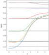 |
Fig. 1. Variation with frequency of the normalized source function, for different values of the optical depth at line center across the atmosphere. Dashed lines indicate the (constant with frequency) CRD values at τ = 0, 1, 10, 100, 103, 104 for comparison, where both SCRD and S(x = 0) increase with τ. It satisfactorily reproduces the standard PRD results using Hummer’s RI − A (see also Hummer 1969, Fig. 1c). |
Even using our simple iterative scheme, we recover easily the Hummer (1969) “historic” solutions. We could also check that the relative error on S(x, τ) between our new scheme versus similar results obtained on a “frequency by frequency” basis (hereafter, FBF; see Paletou & Auer 1995) for RI − A never exceeds 4% with a more typical mean value around 1.3% (for this validation, we used FBF with a six-node Gauss-Legendre angular quadrature).
To achieve this level of accuracy, we computed the CRD solution using the ALI iteration until the maximum relative error on the source function was better than 10−4. The new cycle was then iterated up to a maximum relative error on the frequency dependent source function of 3 × 10⁻⁴.
In Fig. 2, we display the emission profile ψ(x, τ) for different optical depths τ across the atmosphere. These are “naturally” computed using our approach, and without the need for any a priori given redistribution function. The only two assumptions we rely on are: (1) that the VDF f1 of the atoms in their ground state is Maxwellian and (2) that the atomic absorption profile is given a priori in the present case of coherent scattering by a Dirac function centered at the frequency, ν0, of the model-spectral line. Then all relevant quantities, down to the velocity distribution function of the excited atoms at every depth into the atmosphere, are computed consistently with the successive evaluation of the radiation field.
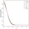 |
Fig. 2. Dependence of the emission profiles ψ(x, τ) on various optical depths across the atmosphere. Top-right frame gives the correspondence between τ at line center and the color of the relevant profile. The distribution is computed self-consistently with the radiation, without the need for any a priori given redistribution function. |
Indeed, we can display, as shown in Fig. 3, a more original sample of the ratios f2(u, τ)/fM(u) for different optical depths, as considered in Fig. 2. In the present paper, we consider the emission profile ψ(x, τ) and, thereby, the source function S(x, τ) to be independent of the polar angles of the radiation field. Therefore, we prefer to illustrate the normalized VDF of the excited atom that depends only on the modulus of velocity, u. This is obtained by integrating f2(u, τ) given by Eq. (3) over atomic velocity directions, namely, dΩu. Important deviations from Maxwellian can be identified, typically for u > 2, and close to the non-illuminated surface of the semi-infinite atmosphere. We can easily recover, using our new numerical procedures, the “overpopulation” of f2 at large u values already proven by Borsenberger et al. (1987).
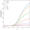 |
Fig. 3. Deviations from Maxwellian illustrated by ratios f2(u, τ)/fM(u) at various optical depths across the atmosphere using the same convention as in Fig. 2. It shows the “overpopulation” of f2 at large u’s. This very information cannot be accessed to, using standard non-LTE approaches. |
Such a material is only accessible using the Oxenius-like formalism that we adopt here. We also note that the de facto neglected potential effects of velocity-changing elastic collisions can only be addressed and studied in that theoretical frame (see details in PP21 and Sect. 7, hereafter). More generally, such additional information could be very valuable for the detailed coupling between the radiation transfer problem and any other physical processes that would take place within an atmosphere and for which the very knowledge of the various VDFs of contributing elements, at different excitation and ionization stages, would be critical.
7. Non-zero velocity-changing elastic collisions
To the best of our knowledge, the preliminary computations related to the present study have only been addressed by Atanackovič et al. (1987) so far. Here, we go a bit further by illustrating in Fig. 4 the dependence of the source function at τ ≈ 1 on the velocity-changing elastic collisions, parameterized as ζ. The model-atmosphere used for this computation is identical to the one adopted in Sect. 6, but we have made vary ζ from 0 to 50. As expected, the source function S(x, τ) ranges between the standard PRD-RI − A solutions when ζ = 0, and the frequency independent CRD values (shown as black dashed line) for increasing values of ζ.
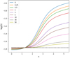 |
Fig. 4. Variation with frequency of the normalized source function at τ ≈ 1, for different values of the velocity-changing elastic collision parameter ζ (indicated in the top-left frame). The model-atmosphere is the same as the one considered in Sect. 6 and Hummer (1969). As expected, successive solutions range between standard PRD-RI − A values (blue) and the limit of the CRD solution (dashed line) for increasing values of ζ. |
As also expected, the numerical problem becomes easier for increasing values of ζ. Effects of velocity-changing elastic collisions will be discussed in more details in another devoted study.
8. Finite slab case
Among the many potential applications at hand, we are particularly interested in the radiative modeling of isolated and illuminated finite slabs. As an example of the anticipated effects, we simulated a 1D plane parallel horizontal slab strongly irradiated asymmetrically, however, only from below. This mimics the radiative modelling of a “cold filament” suspended above a stellar disk (see e.g., Paletou 1997).
We used a 33-point optical depth grid, logarithmically spaced away from open surfaces (using an initial δτ = 0.01) as well as symmetric around a midslab depth set at τ1/2 = 500. For this example we also set ε = 10−4 and ζ = 0. External illumination is applied only at the bottom surface, using a flat profile of normalized intensity of Iext. = 3.
Figure 5 displays values of the normalized VDF f2(u, τ)/fM(u) for optical depth values, counted from the top surface, of τ = 0.58 and τ = 1.15, that is, around the critical value of 1 and at midslab. The quite strong external illumination that we applied generates very significant departures of f2 from Maxwellian, especially at u > 2 again – but greater than what we had already identified for the semi-infinite atmosphere case.
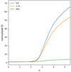 |
Fig. 5. Deviations from Maxwellian illustrated by the changes of the normalized f2 at various optical depths (mentioned in the top-left frame) across an asymmetrically and strongly illuminated finite slab of total depth τ = 103. Largest amplitudes are for these two values around τ = 1, while smaller but significant deviations are still noticeable at midslab (τ = 500). |
9. Discussion and conclusion
We conducted a first critical evaluation of new numerical procedures in radiative transfer for the solution of the “full non-LTE” problem. The results were validated by reproducing both CRD and standard PRD with Hummer’s RI − A (Hummer 1962, 1969), allowing us to move forward in several new directions.
After the very first computations shown here, we shall also be able to evaluate further and in more detail the additional effects of potential velocity-changing elastic collisions with different set of “classic” parameters. In addition, finite slab models, with different conditions of external illumination, can also be considered. Such cases lead to more significant departures from Maxwellian than what happens for semi-infinite slabs, as indicated by our preliminary filament-like computation. Relevant astrophysical “objects” should range from solar prominences to circumstellar environements, for instance.
The next obvious step is to modify the atomic absorption description for the more realistic case of natural broadening of the upper level of the transition. It would go beyond the previous studies of Borsenberger et al. (1987) and Atanackovič et al. (1987), which were limited to “pure” Doppler broadening. Therefore, a Lorentzian profile for atomic absorption will be used. This will also require us to implement modifications to the original formalism of Oxenius for that case, following Bommier (1997) approach, as discussed in PP21. This will be suitable for a preliminary study of resonance lines such as Lyman α of H I. The successive computations of Voigt-like profiles at every iterative step, according to the departures of f2 to Maxwellian, and throughout the whole atmosphere will certainly benefit from the numerical scheme proposed by Paletou et al. (2020). This may also require us to implement and validate a more robust iterative scheme, more likely inspired by the so-called FBF scheme proposed by Paletou & Auer (1995).
Then we shall proceed with the consideration of at least an additional distribution, either for another excited state or for free electrons. This should lead to an alternative, less heuristic approach to the so-called “cross-redistribution” model for the multi-level atoms case (see e.g., Milkey et al. 1975; Hubeny & Lites 1995; Sampoorna & Nagendra 2017).
In the present study, following PP21 and Oxenius (1986) we do not consider departure of the VDF of the fundamental state of the atom from Maxwellian. This is a realistic assumption in the so-called “weak radiation field regime” when stimulated emission can be neglected, leading to a “natural population” of the lower level. This is also the case for an atomic ground level of infinite lifetime.
Acknowledgments
M.S. acknowledges the support from the Science and Engineering Research Board (SERB), Department of Science and Technology, Government of India via a SERB-Women Excellence Award research grant WEA/2020/000012.
References
- Atanackovič, O., Borsenberger, J., Oxenius, J., & Simonneau, E. 1987, J. Quant. Spectrosc. Radiat. Transf., 38, 427 [CrossRef] [Google Scholar]
- Bommier, V. 1997, A&A, 328, 706 [NASA ADS] [Google Scholar]
- Borsenberger, J., Oxenius, J., & Simonneau, E. 1986, J. Quant. Spectrosc. Radiat. Transf., 35, 303 [NASA ADS] [CrossRef] [Google Scholar]
- Borsenberger, J., Oxenius, J., & Simonneau, E. 1987, J. Quant. Spectrosc. Radiat. Transf., 37, 331 [NASA ADS] [CrossRef] [Google Scholar]
- Hubeny, I., & Lites, B. 1995, ApJ, 455, 376 [NASA ADS] [CrossRef] [Google Scholar]
- Hubeny, I., & Mihalas, D. 2014, Theory of Stellar Atmospheres: An Introduction to Astrophysical Non-equilibrium Quantitative Spectroscopic Analysis (Princeton: Princeton University Press) [Google Scholar]
- Hummer, D. G. 1962, MNRAS, 125, 21 [Google Scholar]
- Hummer, D. G. 1969, MNRAS, 145, 95 [NASA ADS] [CrossRef] [Google Scholar]
- Lambert, J., Paletou, F., Josselin, E., & Glorian, J.-M. 2016, Eur. J. Phys., 37, 015603 [Google Scholar]
- Milkey, R. W., Shine, R. A., & Mihalas, D. 1975, ApJ, 199, 718 [NASA ADS] [CrossRef] [Google Scholar]
- Oxenius, J. 1986, Kinetic Theory of Particles and Photons: Theoretical Foundations of non-LTE Plasma Spectroscopy (Berlin: Springer) [CrossRef] [Google Scholar]
- Paletou, F. 1997, A&A, 317, 244 [NASA ADS] [Google Scholar]
- Paletou, F., & Auer, L. H. 1995, A&A, 297, 771 [NASA ADS] [Google Scholar]
- Paletou, F., & Peymirat, C. 2021, A&A, 649, A165 [NASA ADS] [CrossRef] [EDP Sciences] [Google Scholar]
- Paletou, F., Bommier, V., & Faurobert, M. 1999, in Solar polarization, eds. K. N. Nagendra, & J. O. Stenflo (Netherlands: Kluwer) [Google Scholar]
- Paletou, F., Peymirat, C., Anterrieu, E., & Böhm, T. 2020, A&A, 633, A111 [EDP Sciences] [Google Scholar]
- Sampoorna, M., & Nagendra, K. N. 2017, ApJ, 838, 95 [NASA ADS] [CrossRef] [Google Scholar]
- Sampoorna, M., Nagendra, K. N., & Frisch, H. 2011, A&A, 527, A89 [NASA ADS] [CrossRef] [EDP Sciences] [Google Scholar]
All Figures
|
Fig. 1. Variation with frequency of the normalized source function, for different values of the optical depth at line center across the atmosphere. Dashed lines indicate the (constant with frequency) CRD values at τ = 0, 1, 10, 100, 103, 104 for comparison, where both SCRD and S(x = 0) increase with τ. It satisfactorily reproduces the standard PRD results using Hummer’s RI − A (see also Hummer 1969, Fig. 1c). |
| In the text | |
|
Fig. 2. Dependence of the emission profiles ψ(x, τ) on various optical depths across the atmosphere. Top-right frame gives the correspondence between τ at line center and the color of the relevant profile. The distribution is computed self-consistently with the radiation, without the need for any a priori given redistribution function. |
| In the text | |
|
Fig. 3. Deviations from Maxwellian illustrated by ratios f2(u, τ)/fM(u) at various optical depths across the atmosphere using the same convention as in Fig. 2. It shows the “overpopulation” of f2 at large u’s. This very information cannot be accessed to, using standard non-LTE approaches. |
| In the text | |
|
Fig. 4. Variation with frequency of the normalized source function at τ ≈ 1, for different values of the velocity-changing elastic collision parameter ζ (indicated in the top-left frame). The model-atmosphere is the same as the one considered in Sect. 6 and Hummer (1969). As expected, successive solutions range between standard PRD-RI − A values (blue) and the limit of the CRD solution (dashed line) for increasing values of ζ. |
| In the text | |
|
Fig. 5. Deviations from Maxwellian illustrated by the changes of the normalized f2 at various optical depths (mentioned in the top-left frame) across an asymmetrically and strongly illuminated finite slab of total depth τ = 103. Largest amplitudes are for these two values around τ = 1, while smaller but significant deviations are still noticeable at midslab (τ = 500). |
| In the text | |
Current usage metrics show cumulative count of Article Views (full-text article views including HTML views, PDF and ePub downloads, according to the available data) and Abstracts Views on Vision4Press platform.
Data correspond to usage on the plateform after 2015. The current usage metrics is available 48-96 hours after online publication and is updated daily on week days.
Initial download of the metrics may take a while.