© The Authors 2025

1 Introduction

The standard multi-level non-LTE (non-local thermodynamic equilibrium) radiative transfer problem is at the very heart of the interpretation of spectra from astrophysical objects such as stars, circumstellar discs, molecular clouds, and so on (see Hubeny & Mihalas 2014). While the standard approach, which has been continuously developed since the late 1960s, accounts for deviations of the radiation field and the atomic populations from their equilibrium distributions, it assumes velocity distribution of radiating atoms to be Maxwellian.

Hereafter, we consider the problem of full non-LTE (FNLTE) radiative transfer, which mainly consists of the self-consistent calculation of the velocity distribution functions (VDFs) of massive particles with the radiation field; i.e. the distribution of photons in the atmosphere. In that context, the main numerical burden is to work directly with atomic velocities and therefore solve the kinetic equilibrium equations for each velocity.

The kinetic theory of particles and photons (see Oxenius 1986) on which our approach is based also introduces an additional physical process of atomic velocity-changing collisions, which appear naturally in the Boltzmann equations. Hubeny & Cooper (1986, see also; e.g. Hubeny et al. 1983a,b) studied the consequences of these collisions on the radiative transfer problem in detail (see also the discussion in Sect. 4 of Sampoorna et al. 2024). The multi-level problem was originally formulated by Hubeny et al. (1983a,b, hereafter HOSI and HOSII, respectively; see also Oxenius 1965, 1986) using a semi-classical picture.

Until now, only the two-level FNLTE problem has been solved by Paletou et al. (2023, hereafter PSP23; see also Lagache et al. 2025) for infinitely sharp levels, and by Sampoorna et al. (2024) for naturally broadened excited levels. In the FNLTE multi-level radiative transfer problem, the Boltzmann equation for the VDFs of excited atoms need to be solved simultaneously with the radiative transfer equation for all radiatively allowed transitions. Furthermore, at every iteration we also need to recompute all the macroscopic absorption and emission profiles by convolving the atomic profiles with the relevant VDFs. Clearly, this is a numerically very challenging problem. As a first step, we considered a simple atomic model, namely a three-bound-level atom with zero natural broadening, using most data from Avrett (1968).

The FNLTE formalism for multi-level atoms naturally accounts for both resonance and Raman scattering contribu-tions¹. To incorporate these scattering mechanisms - including the effects of partial redistribution (PRD) for resonance scattering and cross-redistribution (a.k.a. XRD) for Raman scattering - in the standard (in the sense that VDF deviations from Maxwellian are only partially considered) non-LTE multi-level problem an approximate approach was adopted; namely, the absorption profile for all transitions was assumed to be the usual Voigt (or Doppler) profile, and a simplified form of the emission profile derived by HOSII was used (see e.g. Hubeny 1985; Uitenbroek 1989; Paletou & Auer 1995; Sampoorna et al. 2013). We remark that the simplifying assumptions behind this approximate approach were detailed in Hubeny (1985), and their validity remains to be evaluated. However, none of these assumptions are used in our more complete FNLTE approach.

This paper is organised as follows. In Sect. 2, we present the formalism of the FNLTE transfer problem and apply it to the case of a three-bound-level atom with zero natural broadening in Sect. 3. Our new numerical scheme is described in Sect. 4. It is validated against various benchmark solutions in Sect. 5 (and Appendix C). Supplementary material, useful for understanding our tests, is presented in the Appendix B. New results are presented in Sect. 6. Finally, conclusions and future developments are discussed in Sect. 7.

2 The FNLTE multi-level problem

Solving a multi-level radiative transfer problem requires the self-consistent resolution of a set of equations, each of them describing the distribution of particles of different nature: photons and massive particles (atoms, ions, molecules, or electrons). Here, we used the kinetic approach developed by Oxenius (1986, 1965), which was extended by HOSI and HOSII and recently dubbed FNLTE by Paletou & Peymirat (2021). In this formalism, the equations of the transfer problem are all kinetic equations.

2.1 The kinetic equations of photons

The distribution of photons associated with the transition from level i of energy E_i, to a level j of energy E_j, is the specific intensity I_ij. For an unpolarised, time-independent problem in a plane-parallel 1D geometry, this distribution depends on the frequency ν_ij of the photon in the observer’s frame, its direction cosine μ_ij = cos(θ_ij), and the optical depth τ_ij(ν_ij). Its kinetic equation is the usual radiative transfer equation (RTE), which is written, with the convention i < j, as follows: $${\mu }_{ij}\frac{\mathrm{\partial }{I}_{ij}({\nu }_{ij},{\mu }_{ij},{\tau }_{ij})}{\mathrm{\partial }{\tau }_{ij}}=I_{ij}({\nu }_{ij},{\mu }_{ij},{\tau }_{ij})-\frac{{\eta }_{ji}({\nu }_{ij},{\tau }_{ij})}{{\chi }_{ij}({\nu }_{ij},{\tau }_{ij})}.$$(1)

Hereafter, we will not display dependence of relevant quantitie on the optical depth τ_ij without loss of clarity. In the RTE, we introduced the emissivity η_ji and the absorption coefficient χ_ij They depend on the frequency, the optical depth, the direction o propagation and, implicitly, the VDFs of the massive particles knowledge of which is indispensable for the computation of th emission and absorption profiles.

In the following, we assume the isotropy of these quantities², and we write $${\eta }_{ji}({\nu }_{ij})=\frac{h{\nu }_{0,ij}}{4\pi }{n}_j{A}_{ji}{\psi }_{ji}({\nu }_{ij}),$$(2)

and $${\chi }_{ij}({\nu }_{ij})=\frac{h{\nu }_{0,ij}}{4\pi }{n}_i{B}_{ij}{\phi }_{ij}({\nu }_{ij}),$$(3)

where A_ji and B_ij are the Einstein coefficients associated, respectively, with spontaneous emission and radiative absorption; ν_0,ij is the frequency of the i ↔ j transition, and n_i and n_j are the population densities of the i and j excited levels. Strictly speaking, we should also consider the stimulated emission characterised by the Einstein coefficient B_ji. However, in most astrophysical cases (with the exception of masers; see e.g. Gray 2012), n_jB_ji << n_iB_ij, and stimulated emission is therefore considered as ‘negative absorption’. Also, taking this additional phenomenon into account makes it much more difficult to obtain atomic frame absorption and emission profiles (see Sect. 5 of HOSI). Therefore, as a first step, we neglected stimulated emission completely. We also introduced the absorption profile φ_ij and the emission profile ψ_ji in the observer’s frame defined as $${\phi }_{ij}({\nu }_{ij})=\oint \frac{d{\mathrm{\Omega }}_{ij}}{4\pi }\int f_i(\mathit{v}){\alpha }_{ij}({\xi }_{ij})d^3\mathit{v},$$(4)

and $${\psi }_{ji}({\nu }_{ij})=\oint \frac{d{\mathrm{\Omega }}_{ji}}{4\pi }\int f_j(\mathit{v}){\beta }_{ji}({\xi }_{ji})d^3\mathit{v},$$(5)

where β_ji³ and α_ij are the atomic emission and absorption profiles; f_i(ν) and f_j(ν) are the VDFs, normalised to unity for, respectively, atoms in the excited level i and j; ν is the atomic velocity; Ω_ij is the direction of a photon of frequency ν_ij depending on azimuth φ_ij and co-latitude θ_ij; and ξ_ij is the photon frequency in the atomic frame. The latter is directly linked to the frequency in the observer’s frame by the Fizeau-Doppler relationships: $${\xi }_{ij}={\nu }_{ij}-\frac{{\nu }_{0,ij}}{c}\mathit{v}\cdot {\mathit{\Omega }}_{\mathit{i}\mathit{j}}.$$(6)

Solving the RTE and therefore the radiative transfer problem requires knowledge of the dynamic and radiative properties of the atoms: (i) their velocity distribution, f_i, (ii) the atomic densities, n_i, and (iii) the atomic profiles, α_ij and β_ji. Each of these elements are discussed below.

2.2 The kinetic equations of massive particles

Massive particles constituting an atmosphere are also described, as photons, by a distribution (in velocity) governed by a kinetic equation. Apart from their nature, the only properties that distinguish each of these atoms are their speed and direction. Each of them is therefore characterised by its own VDF. The standard radiative transfer, however, deals with the self-consistent determination of the number density of the atoms - i.e. the first moment of these VDFs - together with the radiation field so that nothing is known about these VDFs. On the contrary, our more complete FNLTE approach requires the self-consistent resolution of all the kinetic equations describing all the particles distributions.

In the following, we assume that the temperature of the medium is sufficiently small so that n₁ >> n₂, n₃, ... In that case, atoms are so numerous on the fundamental level that their population varies very slightly with respect to the LTE value, and we consider that their distribution is Maxwellian. We only considered bound-bound radiative and collisional processes. For atoms in excited levels, let F_i = n_i f_i be the distribution associated with the excited level i ≥ 2. The kinetic equation describing their distribution is the Boltzmann equation (we neglected the streaming of particles as argued by Hubeny 1981; for more details, please refer to Paletou & Peymirat 2021): $$C[F_i={\left(\frac{\delta F_i}{\delta t}\right)}_{\mathrm{r}\mathrm{a}\mathrm{d}.}+{\left(\frac{\delta F_i}{\delta t}\right)}_{\mathrm{i}\mathrm{n}\mathrm{e}\mathrm{l}.}+{\left(\frac{\delta F_i}{\delta t}\right)}_{v.\mathrm{c}.\mathrm{c}.}=0.$$(7)

Here, C is the collisional operator composed of three terms of different physical origins: a radiative term (collisions with photons), an inelastic term (collisions with free electrons), and a velocity-changing collision term, i.e. collisions between atoms (this nomenclature was discussed in detail in Sect. 4 of Sampoorna et al. 2024).

Let N_i = n_i f_id³ νdV be the number of atoms at level i contained in a volume d³νdV of the phase space. Per second, N_iA_ij atoms spontaneously emit a photon and deexcite towards a level j < i, and N_iB_ijJ_ij(ν) atoms absorb a photon and are excited to a level j > i. In the phase space, these atoms are destroyed. Here, J_ij(ν) denotes the partial scattering integral for atoms at level i and velocity in the range of (ν, ν + dν), which is defined as $$J_{ij}(\mathit{v})=\int {\alpha }_{ij}({\xi }_{ij})I_{ij}d{\xi }_{ij}.$$(8)

Similarly, the number of atoms created at level i from a level j > i is N_jA_ji, and that from a level j < i is N_jB_jiJ_ij(ν). Finally, the total variation of the number density of atoms at level i in a volume d³ νdV of the phase space, i.e. the distribution F_i = N_i/(d³νdV), resulting from the radiative processes alone, is 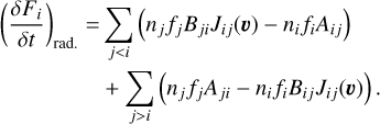$$\begin{array}{r}\hfill \begin{array}{l}{(}_{\frac{\delta F_i}{\delta t}}={\displaystyle \sum _{j<i}}(n_j{f}_j{B}_{ji}{J}_{ij}(\mathit{v})-n_i{f}_i{A}_{ij})\\ +{\displaystyle \sum _{j>i}}(n_j{f}_j{A}_{ji}-n_i{f}_i{B}_{ij}{J}_{ij}(\mathit{v})).\end{array}\end{array}$$(9)

For inelastic collisions, we proceeded in an equivalent way by introducing the collisional excitation and deexcitation coefficients C_ij⁴. We have: 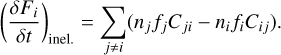$${\left(\frac{\delta F_i}{\delta t}\right)}_{\mathrm{i}\mathrm{n}\mathrm{e}\mathrm{l}.}={\displaystyle \sum _{j\ne i}}(n_j{f}_j{C}_{ji}-n_i{f}_i{C}_{ij}).$$(10)

Velocity-changing collisions also destroy and create particles in phase space. The rate of these collisions is quantified by the parameter Q_V,i for each atomic level (see Oxenius 1986, HOSI, and Paletou & Peymirat 2021). We thus write: $${\left(\frac{\delta F_i}{\delta t}\right)}_{v.\mathrm{c}.\mathrm{c}.}=n_i{Q}_{V,i}[f^M-f_i]$$(11)

where f^M is the Maxwell-Boltzmann velocity distribution defined as $$f^M(\mathit{v})=\frac{1}{v_{\mathrm{t}\mathrm{h}}^3{\pi }^{3/2}}{e}^{-\mathit{v}\cdot \mathit{v}/{\mathit{v}}_{\mathbf{th}}^2},$$(12)

with ν^th being the most probable velocity. The Boltzmann equation is finally written, for level i, as $$\begin{array}{l}{\displaystyle \sum _{j<i}}(n_j{f}_j{B}_{ji}{J}_{ji}(\mathit{v})-n_i{f}_i{A}_{ij})+{\displaystyle \sum _{j>i}}(n_j{f}_j{A}_{ji}-n_i{f}_i{B}_{ij}{J}_{ij}(\mathit{v}))\\ +{\displaystyle \sum _{j\ne i}}(n_j{f}_j{C}_{ji}-n_i{f}_i{C}_{ij})+n_i{Q}_{V,i}[f^M-f_i]=0.\end{array}$$(13)

As we can see from Eq. (13), there is a coupling between each of the VDFs f_i in the Boltzmann equations. This is precisely what the standard non-LTE radiative transfer cannot deal with. We also note that the Boltzmann equations are formally kinetic equilibrium equations (KEE). Integrating over all velocities⁵, we have the equilibrium between all the processes that populate and depopulate the atomic levels in a given space of volume dV. Hereafter, we refer to the following as integrated (and more usual) equations of the kinetic equilibrium or IKEE: $$\begin{array}{l}{\displaystyle \sum _{j<i}}(n_j{B}_{ji}{\mathcal{J}}_{ji}-n_i{A}_{ij})+{\displaystyle \sum _{j>i}}(n_j{A}_{ji}-n_i{B}_{ij}{\mathcal{J}}_{ij})\\ +{\displaystyle \sum _{j\ne i}}(n_j{C}_{ji}-n_i{C}_{ij})=0\end{array}$$(14)

where ${\mathcal{J}}_{ij}$ is the scattering integral, completely equivalent to the standard definition of ${\overline{J}}_{ij}$, and defined as $${\mathcal{J}}_{ij}={\int }_{\mathit{v}}{f}_i(\mathit{v})J_{ij}(\mathit{v})d^3\mathit{v}.$$(15)

2.3 Atomic emission and absorption profiles of a three-bound-level atom

In what follows, we used a model atom with three bound levels. Using phenomenological arguments, HOSI obtained the explicit form of the atomic profiles required to calculate the observer’s frame profiles (see Eqs. (4) and (5)) and the partial scattering integral J_ij(ν) (see Eq. (8)). For the sake of clarity, we briefly recall their main arguments. For more details, we refer the reader to HOSI and HOSII.

First of all, it is important to come back to the notion of natural population. For an ensemble of atoms of the same species, we are interested in a radiative transition from a level b to a level a. Moreover, there is a given radiation field permeating the atmosphere, i.e. a given quantity of photons whose characteristics (frequencies and direction of propagation) are well known. We consider a particular physical process populating the level b. If the number of atoms created in atomic level b is independent of the number of photons already present, then the b → a radiative transition will result in a new distribution of photons that is completely independent of the pre-existing photon distribution in the atmosphere. Thus, we can say that the physical process populating level b leads to its natural population. This is the case for spontaneous emission, inelastic collisions, and velocitychanging collisions. However, radiative absorption depends on the radiation field and so does not naturally populate the atomic levels.

An atomic profile characterises a specific radiative transition; say, b → a. To find an expression for it, we need to study all the transitions and series of transitions that populate level b and, ultimately, lead to the b → a radiative transition. Let c → b be a transition populating level b:

• (i)

  If c naturally populates level b, then the resulting distribution of b → a will be independent of the resulting distribution of c → b. Hence, we need to consider the physical phenomenon involving a single photon, namely the b^* → a radiative transition (where the notation l^* means that level l is naturally populated). To describe it, we use the generalised redistribution function r_ba(ξ_ba) related to the probability that a photon of frequency between ξ_ba and ξ_ba + dξ_ba is involved in the b → a transition.

• (ii)

  If c does not naturally populate level b but is itself naturally populated, we need to consider a two-photon phenomenon ( c^* → b → a). To handle it, we define the conditional probability j_cba(ξ_ba); i.e. the probability that a photon of frequency between ξ_ba and ξ_ba + dξ_ba is involved in the b → a transition, knowing that a photon of frequency between ξ_cb and ξ_cb + dξ_cb was previously involved in the c^* → b transition. This quantity is defined as (see Eq. (4.4) of HOSI): $$j_{cba}({\xi }_{ba})=\frac{\int I_{cb}{r}_{cba}({\xi }_{cb},{\xi }_{ba})d{\xi }_{cb}}{\int I_{cb}{r}_{cb}({\xi }_{cb})d{\xi }_{cb}}.$$(16)

  In this equation, r_cba(ξ_cb ,ξ_ba) is the generalised redistribution function describing the probability that two photons whose frequencies are, respectively, between ξ_cb,ξ_cb + dξ_cb and ξ_ba,ξ_ba + dξ_ba, are engaged in the c^* → b → a transition (see Sect. 3 of HOSI). To understand the meaning of j_cba(ξ_ba), we need to interpret each quantity probabilistically. The specific intensity Icb can be related to the so-called photon number density (see e.g. Hubeny & Mihalas 2014). Thus, we can see the denominator term of Eq. (16) as the total number of photons involved in the c → b transition and the numerator term as the fraction of photons created by the b → a transition that actually comes from the c → b transition.

• (iii)

  If c does not naturally populate the b level and is non-naturally populated by a third transition d* → c, we need to consider a phenomenon involving three photons in the series of transitions d* → c → b → a. To describe such a phenomenon, we should use the conditional probability j_dcba(ξ_ba) defined analogously to Eq. (16).

• (iv)

  It is clear that the d level itself can be populated non-naturally by a given e → d transition, and similarly for e with an f → e transition, and so on. Finally, when a photon is involved in the b → a transition, there will be a given probability that it originally comes from one of the series of transitions previously described. The atomic profile is the probability density describing all these possibilities simultaneously. It is defined as the average of all the series of possible transitions weighted by their occurrence probabilities.

For atoms with three levels, we therefore need to determine three absorption profiles - α₁₂, α₁₃, and α₂₃ - as well as three emission profiles: β₂₁, β₃₁, and β₃₂. The α₁₂ and α₁₃ profiles are the simplest to determine. Since stimulated emission has been neglected, the fundamental level is naturally populated. Consequently, the probability of occurrence of such a phenomenon is certain; only case (i) needs to be taken into account. We therefore have $${\alpha }_{12}=r_{12}({\xi }_{12})$$(17)

and $${\alpha }_{13}=r_{13}({\xi }_{13}).$$(18)

For β₂₁ and α₂₃, we need to take into account all the series of transitions leading to level 2. It can be naturally populated, and we denote prob(→ 2^*) as the relevant probability following HOSI and HOSII notations. This is case (i). It can also be populated non-naturally from the fundamental level, and we express prob(1^* ⇒ 2) as its probability. This is case (ii). Combining these two phenomena, we have (see Eqs. (4.3) and (4.6) of HOSI) $${\alpha }_{23}=\mathrm{p}\mathrm{r}\mathrm{o}\mathrm{b}(\to 2^{\ast })r_{23}+\mathrm{p}\mathrm{r}\mathrm{o}\mathrm{b}(1^{\ast }\Rightarrow 2)j_{123}$$(19)

and $${\beta }_{21}=\mathrm{p}\mathrm{r}\mathrm{o}\mathrm{b}(\to 2^{\ast })r_{21}+\mathrm{p}\mathrm{r}\mathrm{o}\mathrm{b}(1^{\ast }\Rightarrow 2)j_{121}.$$(20)

For β₃₂ and β₃₁, we are interested in the processes populating level 3. We had to take into account the processes which do not naturally populate level 3 from level 2 and therefore treat the cascade 1^* → 2 → 3 → 1 or 1^* → 2 → 3 → 2 (case (iii)). We then have (see Eqs. (4.7) and (4.8) of HOSI) $$\begin{array}{rl}& {\beta }_{31}=\mathrm{p}\mathrm{r}\mathrm{o}\mathrm{b}(\to 3^{\ast })r_{31}+\mathrm{p}\mathrm{r}\mathrm{o}\mathrm{b}(1^{\ast }\Rightarrow 3)j_{131}\\ & +\mathrm{p}\mathrm{r}\mathrm{o}\mathrm{b}(\to 2^{\ast }\Rightarrow 3)j_{231}+\mathrm{p}\mathrm{r}\mathrm{o}\mathrm{b}(1^{\ast }\Rightarrow 2\Rightarrow 3)j_{1231}\end{array}$$(21)

and $$\begin{array}{rl}& {\beta }_{32}=\mathrm{p}\mathrm{r}\mathrm{o}\mathrm{b}(\to 3^{\ast })r_{32}+\mathrm{p}\mathrm{r}\mathrm{o}\mathrm{b}(1^{\ast }\Rightarrow 3)j_{132}\\ & +\mathrm{p}\mathrm{r}\mathrm{o}\mathrm{b}(\to 2^{\ast }\Rightarrow 3)j_{232}+\mathrm{p}\mathrm{r}\mathrm{o}\mathrm{b}(1^{\ast }\Rightarrow 2\Rightarrow 3)j_{1232}.\end{array}$$(22)

For more details on the expressions of ‘prob’ probabilities, we refer the reader to HOSI or Oxenius (1986). Knowledge of these quantities will not be explicitly necessary later on. In this work, we only studied the simplified case of an atom with three infinitely sharp levels. In Sect. 3, we will see how this simplifies the expression of the general atomic profiles given above and, consequently, the whole problem.

3 A three-level atom with infinitely sharp levels

With the exception of the fundamental level, atomic levels are generally broadened in energy. In the theoretical developments of HOS presented above, no assumptions on the atomic model were made. Considering the same physical processes, the assumption of infinitely sharp levels does not degrade the problem, although it does simplify it. However, we warn the reader that this hypothesis is part of a heuristic approach and that the realistic study of an astrophysical atmosphere does not leave us the choice of the atomic model, it imposes it. In fact, it is the physical conditions in which the atoms are immersed and the intrinsic nature of the atoms that dictate the width of the atomic levels (broadened or infinitely sharp). For example, if the conditions under investigation lead to collisional broadening, these physical conditions impose an atomic model. Similarly, if we assume an atom such that levels 4 and 5 are naturally broadened, but levels 2 and 3 are not (e.g. metastable levels), this atomic model must be adopted for a realistic study. Hereafter, we restrict ourselves to an atmosphere composed of atoms with three bound and infinitely sharp levels, neglecting stimulated emission and considering that the VDF associated with the fundamental level is Maxwellian (f₁ ≡ f^M).

3.1 Atomic profiles

To calculate the atomic profiles of a three-level atom, we distinguish five phenomena that ultimately lead to the radiative transition under investigation: (i) absorption or emission of a single photon in a given b → a transition (r_ab terms); (ii) resonance scattering, i.e. absorption and re-emission of a photon in a single line (j_aba terms); (iii) Raman scattering, i.e. absorption and re-emission of a photon in two distinct lines (j_cba terms); (iv) two-photon absorption processes (j₁₂₃ term) and (v) three-photon processes (j_dcba terms). Since our levels are assumed to be infinitely sharp, the probability that a photon involved in a given b → a transition has a frequency ξ_ba ≠ v_0,ba is zero. We then write $$r_{ba}({\xi }_{ba})=\delta ({\xi }_{ba}-{\nu }_{0,ba}),$$(23)

where δ is the Dirac distribution. Resonance scattering was studied by Hummer (1962), which obtained analytical expressions for the redistribution functions r_aba(ξ_ab, ξ_ba). Later, Hubeny (1982) obtained general expressions for all two-photon redistribution functions r_cba(ξ_cb,ξ_ba). For atoms without natural broadening, we have, for the Raman or resonance scattering processes (see Eq. (10.135) of Hubeny & Mihalas 2014), $$r_{cba}({\xi }_{cb},{\xi }_{ba})=\delta ({\xi }_{cb}-{\nu }_{0,cb})\delta ({\xi }_{ba}-{\nu }_{0,ba})=r_{cb}({\xi }_{cb})r_{ba}({\xi }_{ba}).$$(24)

The conditional probabilities j_cba (ξ_ba ) are then written as follows: $$j_{cba}({\xi }_{ba})=\frac{\int I_{cb}{r}_{cb}({\xi }_{cb})r_{ba}({\xi }_{ba})d{\xi }_{cb}}{\int I_{cb}{r}_{cb}({\xi }_{cb})d{\xi }_{cb}}=r_{ba}({\xi }_{ba}).$$(25)

In this study, we did not consider the two-photon absorption process. As discussed in Hubeny & Mihalas (2014, pp. 322-323), this process is negligible in most astrophysical atmospheres. We also neglected all three-photon processes for which redistribution functions were obtained by Hubeny & Oxenius (1987) from quantum mechanical calculations. For α₂₃, for example, the term proportional to j₁₂₃ is assumed to be equal to zero, and therefore α₂₃ = prob( → 2^*)r₂₃. We know that atomic profiles and generalised redistribution functions are normalised to unity because they are probability densities. Hence, to guarantee this condition, we renormalised α₂₃, which gives α₂₃ = r₂₃ . We proceeded in the same way when three-photon processes were neglected.

Finally, for a three-level atom with infinitely sharp levels, each of the six atomic profiles established in Eqs. (17)-(22) can then be written simply, ∀j > i, after renormalisation, as $${\alpha }_{ij}({\xi }_{ij})=r_{ij}({\xi }_{ij})=\delta ({\xi }_{ij}-{\nu }_{0,ij})$$(26)

and $${\beta }_{ji}({\xi }_{ji})=r_{ji}({\xi }_{ji})=\delta ({\xi }_{ji}-{\nu }_{0,ij}).$$(27)

3.2 The multi-level atom problem

Our new problem therefore involves five coupled distributions: three specific intensities, associated with each of the radiatively allowed transitions, and two velocity distributions associated with the two excited levels. We must now jointly solve all the RTEs (see Eq. (1)), together with the IKEE (see Eq. (14)) and the Boltzmann equations (see Eq. (13)). The set of IKEEs is redundant. So, for atoms with three levels, we chose to replace one of the three equations, namely the one associated with the fundamental density level n₁, by the conservation equation n₁ + n₂ + n₃ = n_tot. Thus, solving the IKEE is equivalent to solving the system: $$\left(\begin{array}{ccc}1& 1& 1\\ E_{21}& D_2& E_{23}\\ E_{31}& E_{32}& D_3\end{array}\right)\left(\begin{array}{c}{n}_1\\ n_2\\ n_3\end{array}\right)=\left(\begin{array}{c}{n}_{\mathrm{t}\mathrm{o}\mathrm{t}}\\ 0\\ 0\end{array}\right),$$(28)

with $$E_{ij}=A_{ji}+B_{ji}{\mathcal{J}}_{ji}+C_{ji}$$(29)

and $$D_i=-{\displaystyle \sum _{j\ne i}}(A_{ij}+B_{ij}{\mathcal{J}}_{ij}+C_{ij}).$$(30)

In the above equations, we (numerically) assume that A_ij = 0 for i < j and B_ij = 0 for i > j.

Solving Boltzmann equations means solving a set of three equations, one of which is trivial (f₁ = f^M). We then have $$\left(\begin{array}{ccc}1& 0& 0\\ e_{21}& d_2& e_{23}\\ e_{31}& e_{32}& d_3\end{array}\right)\left(\begin{array}{c}{f}_1(\mathit{v})\\ f_2(\mathit{v})\\ f_3(\mathit{v})\end{array}\right)=\left(\begin{array}{c}1\\ -n_2{Q}_{V,2}\\ -n_3{Q}_{V,3}\end{array}\right)f^M(\mathit{v}),$$(31)

with $$e_{ij}=n_j(A_{ji}+B_{ji}{J}_{ji}(\mathit{v})+C_{ji})$$(32)

and $$d_i=-n_i(Q_{V,i}+{\displaystyle \sum _{j\ne i}}(A_{ij}+B_{ij}{J}_{ij}(\mathit{v})+C_{ij})).$$(33)

The choice of the atomic and scattering models does not directly affect the form of these equations. However, their ingredients do depend explicitly on them: the absorption and emission profiles in the observer’s frame φ_ij and ψ_ji and the partial scattering integrals J_ij(ν), given, respectively, by Eqs. (4), (5), and (8). For infinitely sharp levels, the emission and absorption profiles take the form (see Appendix A) $${\psi }_{ji}(x_{ji})=\frac{1}{2{\mathrm{\Delta }}_{ji}}{\int }_{|x_{ji}|}^{\mathrm{\infty }}{f}_j(u)udu$$(34)

and $${\phi }_{ij}(x_{ij})=\frac{1}{2{\mathrm{\Delta }}_{ij}}{\int }_{|x_{ij}|}^{\mathrm{\infty }}{f}_i(u)udu,$$(35)

together with $$J_{ij}(\mathit{u})=\oint \frac{d{\mathrm{\Omega }}_{ij}}{4\pi }\int \delta (x_{ij}-\mathit{u}\cdot {\mathit{\Omega }}_{\mathit{i}\mathit{j}})I_{ij}d{x}_{ij}.$$(36)

In the equations above, we introduce the reduced frequency x_ij = (ν_ij - v_0,ij)/Δ_ij; the normalised velocity u = u/u_th⁶; and the Doppler width ${\mathrm{\Delta }}_{ij}=({\nu }_{0,ij}/c)v_{\mathrm{t}\mathrm{h}}$. We also note that f_i(u) is the modulus of the VDF f_i(u), i.e. its integration over all the directions Ω_u of the atoms. Finally, it is easy to show that φ₁₂ and φ₁₃ are given by the mere Doppler profile, $${\phi }_{ij}(x_{ij})=\frac{1}{{\mathrm{\Delta }}_{ij}}\times \frac{1}{\sqrt{\pi }}{e}^{-x_{ij}^2},$$(37)

because f₁ = f^M. A priori, all the other profiles will be different, and only a self-consistent resolution of the RTE, IKEE, and Boltzmann equations will make it possible to obtain an expression that is physically consistent with the FNLTE approach to radiative transfer.

4 Numerical strategy

In this section, we present our numerical strategy for solving the FNLTE problem for three infinitely sharp bound-level atoms. We first initialised the iterative process to the multi-level CRD solution with the MALI method of Rybicki & Hummer (1991, hereafter the MALI-CRD method; see also Paletou & Lagache 2025). Then, we successively updated each of the radiative quantities using the following very simple strategy:

• 0: Initialise with a MALI-CRD solution, which gives the population densities n₁, n₂, and n₃ and therefore the CRD source functions.

• 1: For each of the transitions, calculate the emission and absorption coefficients, η_ji, χ_ij, using Eqs. (2) and (3).

• 2: Calculate the source function S_ij: $$S_{ij}(x_{ij})=\frac{{\eta }_{ji}(x_{ij})}{{\chi }_{ij}(x_{ij})}.$$(38)

• 3: Knowing the source function at all optical depths, compute photon distributions I_ij for each of the transitions.

• 4: Compute the partial scattering integrals, J_ij(u), given by Eq. (36), using the current VDF (a Maxwellian is adopted for the first iteration; see also Sect. 4 of PSP23).

• 5: Compute scattering integrals, ${\mathcal{J}}_{ij}$, using Eq. (15).

• 6: Update all populations, n_i , by solving the IKEE system in Eq. (28).

• 7: Update the velocity distributions, f_i, by solving the system in Eq. (31) at each optical depth and atomic velocity u.

• 8: Update φ_ij and ψ_ji profiles for each of the radiatively allowed transitions using Eqs. (35) and (34), and return to Step 1.

The output of this iterative process is a self-consistent determination of all the photon and massive particle distributions.

5 Validation

Since the multi-level FNLTE radiative transfer problem was never fully addressed before, we proceeded with the validation of our calculations through several indispensable verification steps. Furthermore, since we considered the restricted case of a three-level atom with infinitely sharp levels and neglected velocity-changing collisions (see below), the numerical solutions presented here essentially validate our numerical scheme and do not represent the real spectral lines of hydrogen formed in a stellar atmosphere.

All the solutions presented in this sections are calculated with a common set of parameters taken from Avrett (1968, Sect. 9.A; see also the code shared by Paletou & Lagache 2025)⁷. We considered an isothermal atmosphere composed of a three-bound-level hydrogen atom in a 1D, semi-infinite, plane-parallel geometry having a maximum total optical depth of τ_max = 10¹⁴ for the transition 1 ↔ 2. We neglected the effects of velocitychanging collisions, i.e. Q_V = 0 (however, Q_V = 0 adds no numerical difficulties). We sample the optical depth scale with a logarithmic grid using four points per decade extending from 0 to τ_max, with an initial step of 10⁻³. Integration over μ is performed using a six-point Gauss-Legendre quadrature. Integration over the azimuths (required to calculate J_ij(u) - see PSP23) was performed using a ten-point rectangular quadrature. Finally, grids of reduced frequency, x, and normalised velocity, u, are identical and extend from 0 to x_max = u_max = 4 with a step of 0.1. Velocity and frequency integrations were performed with trapezoidal quadrature. Each solution computed with our FNLTE code was obtained after 75 iterations, and the process is always initialised by the CRD solution, obtained after 100 iterations of the MALI-CRD method. Finally, for quantitative comparison purposes, we introduce the following relative error term, defined for each optical depth and frequency, $$\mathrm{E}\mathrm{r}{\mathrm{r}}_{ij}^{\text{rel}}=\left|\frac{S_{ij}^{\text{FNLTE}}-S_{ij}^{\text{ref}}}{S_{ij}^{\text{ref}}}\right|,$$(39)

between our FNLTE source functions S_ij and reference solutions described hereafter.

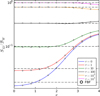Fig. 1 Frequency variation of normalised source function S12 of 1 ↔ 2 line at different optical depths τ for a two-level atom. Horizontal dashed black lines show CRD solutions for τ = 0, 1, 10, 100, 103, 104. We compare FNLTE results (coloured lines) with Hummer’s PRD results (black open circle). CRD and PRD solutions were computed using the ALI and FBF methods, respectively. Clearly, we accurately recover the results presented by Hummer (1969) and PSP23.

5.1 Benchmarking against a two-level atom in PRD

The first step in validating our multi-level code is to reduce it to a two-level atom problem with coherent scattering in the atom’s frame. PSP23 showed that when Q_V = 0 it is equivalent to Hummer’s results for PRD R_I-A (Hummer 1962). Fig. 1 displays the source functions for 1 θ 2 line, obtained with our FNLTE method (coloured lines) and compared to the reference R_I-A PRD solution (open black circles) calculated using the FBF method (Paletou & Auer 1995). The mean of the relative error between these solutions is ≈0.31%. We are also able to reproduce the results obtained by PSP23 for the f₂ distribution function.

5.2 Benchmarking against multi-level CRD

Next, by forcing, in our new three-level FNLTE code, that f₁ = f₂ = f₃ = f^M, we recover the well-known results of MALI-CRD for Avrett’s hydrogen case (Avrett 1968, see also Paletou & Léger 2007). In Fig. 2, we show the optical depth variations of the source function calculated for each of the three lines using our multi-level FNLTE code and the MALI-CRD method. Mean relative errors of about 0.12% for 1 ↔ 2, 0.33% for 1 ↔ 3, and 0.32% for 2 ↔ 3 lines are reported, and they more likely come from completely different numerical schemes.

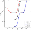Fig. 2 Optical depth variations of normalised source functions for each line of a three-level hydrogen atom in CRD. Our three-level FNLTE code (coloured lines) accurately reproduces reference solutions (open black circle) computed with MALI-CRD.

5.3 Benchmarking against XRD

On the basis of the theoretical work of HOSI & HOSII, the FNLTE approach of radiative transfer presented in Sect. 2 appears, at present, as the most complete approach (however, the QED approach of Bommier 2016 goes beyond the semi-classical picture of HOS formalism used here). In the past, indeed, numerous attempts have been made to incorporate it in more advanced radiative models, but with several simplifying assumptions. As a result of this, none of them could solve all the kinetic equations self-consistently with the RTE. The case where only resonance scattering is taken into account, namely the case of standard PRD, was studied by Hubeny (1985). When Raman scattering is taken into account, we speak of ‘cross-redistribution’ (this term was used by Milkey et al. 1975 to describe this scattering process) or XRD (e.g. Hubeny & Lites 1995; Sampoorna et al. 2013; Uitenbroek 1989). In all cases, these approaches were incomplete, with persisting approximations: (i) all absorption profiles and (ii) scattering integrals ${\mathcal{J}}_{ij}$ were calculated using Maxwellian VDFs, (iii) d_i ≈ n_i(D_i - Q_V,i)⁸ in the Boltzmann equations, and (iv) there is no coupling between the VDFs; in other words, to calculate f_i, we assumed that $f_j=f^M\mathrm{\forall }j\ne i$. Considering these assumptions, the Boltzmann equations presented in Eq. (31) reduce to (assuming Q_V = 0 again), for all atomic excited levels, $$f_2\approx \frac{f^M}{n_2{P}_2}\{[n_3(A_{32}+C_{32})+n_1{C}_{12}]+n_1{B}_{12}{J}_{12}(\mathit{u})\}$$(40)

and $$f_3\approx \frac{f^M}{n_3{P}_3}\{[n_1{C}_{13}+n_2{C}_{23}]+n_1{B}_{13}{J}_{13}(\mathit{u})+n_2{B}_{23}{J}_{23}(\mathit{u})\},$$(41)

where P_i are defined as $$P_i={\displaystyle \sum _{j\ne i}}(A_{ij}+B_{ij}{\mathcal{J}}_{ij}+C_{ij}).$$(42)

From these analytical expressions, we can deduce a general expression for the emission profiles (see Appendix B for more details): $$\begin{array}{cc}{\psi }_{ji}=& \frac{{\phi }_{ij}^{\ast M}}{n_j{P}_j}\{n_i{B}_{ij}{\overline{J}}_{iji}^M+{\displaystyle \sum _{\begin{array}{c}l\ne i,j\\ l<j\end{array}}}{n}_l{B}_{lj}{\overline{P}}_{lji}^M\\ & +[n_i{C}_{ij}+{\displaystyle \sum _{k\ne i,j}}{n}_k(A_{kj}+C_{kj})]\},\end{array}$$(43)

where the notation X^M means that quantities were calculated using a Maxwellian VDF, in particular for the generalised redistribution functions, R_ijk, contained in the definition of the diffusion integrals J_iji and P_lji. This last equation is completely equivalent to Eq. (11) of Sampoorna et al. (2013) obtained in XRD; i.e. considering resonance and Raman scattering effects. Whether one works directly with the emission profiles (XRD) or solves the uncoupled kinetic equations (namely Eqs. (40) and (41)) self-consistently with the transfer equations, respective results should be identical. We show that, within the framework of the approximations presented above, there is an equivalence between our FNLTE formalism and the XRD formalism used by Sampoorna et al. (2013), whose numerical implementation is inspired by the MALI-PRD method developed by Paletou (1995).

The source functions obtained with these two methods are shown in Figs. 3 and 4, respectively, for the 1 ↔ 3 and 2 ↔ 3 lines. For the 1 ↔ 3 line, we measure a mean relative error between our degraded FNLTE code solution and the XRD solution of about 0.23%. For 2 ↔ 3, it is about 0.37%. We chose not to show the source function associated with the 1 ↔ 2 line, as it differs only slightly from the solution shown in Fig. 1 (a relative maximum difference of 4.6% with respect to the two-level atom solution). However, XRD results are very well reproduced for this line with our FNLTE code, with a mean relative error between these two solutions of about 0.23%.

In Fig. 4, at the surface and at high frequency, we observe an overshoot; i.e. $S_{23}/{\mathcal{B}}_W>1$. The possibility that we are facing a numerical problem has been explored, in particular because we explored regions where the optical depths become very tiny. However, this feature is reproduced identically by the two different numerical methods. Furthermore, as the numerical problems remain identical, no similar behaviour has been observed in any of the other cases studied (such as MALI-CRD and MALI-PRD; the latter is discussed in Appendix C). This characteristic seems to be specific to XRD, which suggests that the consistency of some of its assumptions would need to be discussed further. However, as we see in Sect. 6, this artefact disappears when one finally deals with the complete problem. The above-mentioned -and very satisfactory - tests now lead us with confidence towards new results, using the full description.

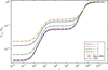Fig. 3 Optical depth variations of normalised source functions for the 1 ↔ 3 line of a three-level hydrogen atom in the frame of XRD approximation. We compare FNLTE results (coloured lines) for various frequencies x = 0, 1, 2, 3, 4 with XRD reference solutions (open black circle) computed using the MALI-XRD method of Sampoorna et al. (2013). The dashed black line shows the CRD solution computed using the MALI-CRD method.

Fig. 4 Same as Fig. 3, but for 2 ↔ 3 line.

6 New results

Hereafter, we used the same model and parameters as the ones used for our previous tests; in particular, velocity-changing collisions continue to be neglected (although their treatment does not present any numerical additional difficulty). Firstly, the S₁₂ source function for the 1 ↔ 2 line changes very slightly compared to the results obtained by PSP23 with a two-level atom with a mean relative error between these solutions of the order of 1.92%. This can be explained by the fact that atomic levels are much less populated when their energy is higher. In other words, we have n₁ >> n₂ >> n₃ >> ... Thus, the source function for the 2 ↔ 1 transition is largely dominated by radiative processes populating level 2 from level 1 and vice versa. The impact of multi-level modelling on this line is therefore marginal. On the other hand, the 1 ↔ 3 and 2 ↔ 3 lines are substantially affected by FNLTE effects. In Figs. 5 and 6, we show the S₁₃ and S₂₃ source functions obtained for these lines. Differences can be seen at the surface with XRD, comparing Figs. 5 and 6, respectively, with Figs. 3 and 4. We know that it is at the surface that non-LTE effects are more pronounced. It is therefore not surprising that any change in the approach, describing all deviations from LTE, modifies the characteristics of the atmosphere in this region. As we explain in the previous section, the overshoot observed using XRD for the S₂₃ source function now disappears. This is because the frequency variations of the source function are mainly due to the ratio between the emission and the absorption profile: $${\rho }_{ij}(x)=\frac{{\psi }_{ji}(x)}{{\phi }_{ij}(x)}.$$(44)

With XRD, we have ρ₂₃ >> 1 precisely in this region close to the surface and far from the line centre where the overshoot is observed, as can be seen from the left panel of Fig. 7. According to XRD assumptions, all absorption profiles are calculated using a Maxwellian. However, we see in Sects. 2 and 3 that the absorption profile φ₂₃ should also be determined in a self-consistent way with all the other radiative quantities; i.e. calculated with f₂ ≠ f^M. It therefore seems contradictory to use f₂ to determine the emission profile, ψ₂₁, but ignore this fact for the absorption profile, φ₂₃. This suggests that XRD’s assumption about absorption profiles is largely responsible for the overshoot. This characteristic is no longer present when φ₂₃ is self-consistently calculated, and, quantitatively, we can see that ρ₂₃ decreases significantly in the very same regions (see the right panel of Fig. 7).

A more detailed examination of the influence of each of the four XRD assumptions (see Sect. 5.3) taken separately shows that the assumption on absorption profiles has a major impact on the S₂₃ source function. Quantitatively, we measure a mean relative difference between the solution thus obtained and the FNLTE solution of the order of 65%. Qualitatively, and as discussed above, this assumption considerably increases the S₂₃ source function in the areas where the overshoot is observed in XRD. However, the amplitude of the overshoot is increased by a factor ≈2. This hypothesis alone does not fully explain this behaviour. Another XRD hypothesis must therefore have the opposite effect, by reducing the S₂₃ source function near the surface and at high frequency. This is precisely the qualitative effect of the hypothesis on the coupling between the VDFs in the Boltzmann equations. The inclusion of these two assumptions alone explains the appearance of this overshoot, with a maximum relative deviation between the solution thus obtained and the XRD solution of the order of ≈3%. The other assumptions have a much smaller impact, of the order of a few percent on average. However, what is more important is that the FNLTE approach allows us to get rid of all these assumptions and solves the XRD overshooting issue. It is important to note that the XRD overshooting problem seen in the present work (see Fig. 4) is also due to the use of a three-level model atom with infinitely sharp levels. More specifically, the overshoot in S₂₃ from the XRD hypothesis is a pathological feature of R_I (Hummer 1962) and P_I (Hubeny 1982) and does not occur with R_II and P_II, which include the natural broadening of energy levels. Indeed, the latter has been verified using the MALI-XRD method of Sampoorna et al. (2013). Moreover, in a more realistic case including more atomic levels, one would expect to observe a strong influence of the higher levels on level 3, modifying the behaviour near the surface.

Finally, it has been emphasised throughout this paper that the FNLTE approach for radiative modelling deals not only with the possible deviations of the radiation field and atomic populations from their equilibrium distributions, but also for the deviation of the VDFs from Maxwellian. Therefore, in addition to the usual source functions, we are now able to obtain all VDFs, f_i ≠ f^M, of the excited levels. As S₂₁, we find that f₂ varies only slightly from the two-level results previously obtained by PSP23. Indeed, we measure a mean relative deviation of 0.084% between these two solutions. However, the velocity distribution associated with level 3 is a new feature introduced by the FNLTE approach, as displayed in Fig. 8. The higher the atomic velocity modulus u is, the more f₃ deviates from the Maxwellian. In deeper layers, as f₃ → f^M the atmosphere tends to be thermalised. We also note that the variations in f₃ are very similar to those in ρ₂₃ (XRD), which is perfectly understandable given the explicit dependence of the profiles on the distribution functions (especially because ψ₃₂ is calculated using f₃).

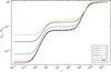Fig. 5 Optical depth variations of normalised source functions for 1 ↔ 3 line of a three-bound-level hydrogen atom. It shows FNLTE results (coloured lines) obtained for various frequencies: x = 0, 1, 2, 3, 4. The dashed black line represents the MALI-CRD solution.

Fig. 6 Same as Fig. 5, but for 2 ↔ 3 line.

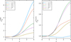Fig. 7 Frequency variations of ρ23 ratio for 2 ↔ 3 line of a three-bound-level hydrogen atom. We show the XRD (left plot) and FNLTE (right plot) results obtained for different optical depths: τ = 10−12, 10−10, 10−8, 10−5, 1.

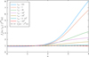Fig. 8 Normalised atomic velocities variations of f3 velocity distribution of the second excited level of a three-bound-level hydrogen atom. Results (coloured lines) were obtained for different optical depths: τ31 = 0.5, 1, 10, 102, 108, 5 · 108, 1012. The dashed black line shows the Maxwellian limit f3(u) = fM(u).

7 Conclusions

Although they were thoroughly formulated more than forty years ago by Hubeny et al. (1983a,b) (see also Oxenius 1986), FNLTE effects for a multi-level atom had never been computed before the present study. As a first step, we restricted ourselves to a simple three-bound-level model atom, based on parameters initially provided by Avrett (1968), and infinitely sharp levels for several benchmark purposes.

As our preliminary solutions to the multi-level FNLTE problem cannot be directly compared with other studies, we verified our ability to reproduce several ‘degraded’ problems with accuracy. This also led us to point out some inconsistencies of the quite advanced still XRD modelling.

The level of realism of the atomic and scattering models will need to be improved in order to take into account the natural broadening of excited atomic levels. However, the major conceptual jump from two to three or more levels has already been made, and the Sampoorna et al. (2024) step will be generalised further.

In the longer term, we could also consider non-Maxwellian free electrons in a self-consistent way as other massive particles. Cases where stimulated emission is not negligible could also be explored, although this would involve major changes in the calculation of atomic profiles.

Finally, we are aware that realism comes at a high computational price. For this purpose, we need to develop a more efficient numerical scheme. However, another study of ours (Lagache et al. 2025) shows that it is possible to adapt approximate operator methods (see e.g. Hubeny 2003; Paletou & Auer 1995) to the two infinitely-sharp-level FNLTE problem. Therefore, in the near future, a robust and convergent method similar to these ones will be adapted to our new multi-level, multi-distribution problem.

Acknowledgements

T. Lagache is kindly supported by a ‘PhD booster’ grant by the Toulouse Graduate School of Earth and Space Sciences (TESS; https://tess.omp.eu/). Authors thank Prof. Ivan Hubeny for very critical and insightful comments.

Appendix A Derivation of observer’s frame profiles

The absorption and emission profiles in the observer’s frame are given by the Eqs. (4) and (5). For infinitely sharp levels, we have given the form of the atomic profiles in the Eqs. (26) and (27). Thus, with j > i, we write (for example for ψ but the calculation is completely analogous for φ): $${\psi }_{ji}({\nu }_{ji})=\oint \frac{d{\mathrm{\Omega }}_{ji}}{4\pi }\int f_j(\mathit{u})\delta ({\xi }_{ji}-{\nu }_{0,ij})d^3\mathit{u}.$$(A.1)

Using the definitions of the reduced frequency x_ji, the normalised velocity u and the Doppler-Fizeau effect given in Eq. (6), we obtain: $${\psi }_{ji}=\frac{1}{{\mathrm{\Delta }}_{ji}}\oint \frac{d{\mathrm{\Omega }}_{ji}}{4\pi }\int f_j(\mathit{u})\delta (x_{ji}-\mathit{u}\cdot {\mathbf{\Omega }}_{ji})u^{2}dud{\mathrm{\Omega }}_u.$$(A.2)

Noticing that: $$\oint \frac{d{\mathrm{\Omega }}_{ji}}{4\pi }\delta (x_{ji}-\mathit{u}\cdot {\mathbf{\Omega }}_{ji})=\frac{1}{2u}H(u-|x_{ji}|),$$(A.3)

with H the Heaviside function, then: $${\psi }_{ji}(x_{ji})=\frac{1}{2{\mathrm{\Delta }}_{ji}}{\int }_{|x_{ji}|}^{\mathrm{\infty }}{f}_j(u)udu.$$(A.4)

Appendix B Derivation of a general expression for emission profiles in the XRD approximations

The aim here is to obtain a general expression for the emission profiles within the framework of the approximations of the so-called XRD approach of the non-LTE radiative transfer. These approximations are described in detail in Sect. 5.3. Before applying this set of assumptions, we propose a more general formulation based on the kinetic equations given in Eq. (13). For this purpose, we rewrite these equations as: $$n_i{\mathrm{\Pi }}_i(\mathit{u})f_i=L_i,$$(B.1)

with, $${\mathrm{\Pi }}_i(\mathit{u})=Q_{V,i}+{\displaystyle \sum _{j\ne i}}[{\tilde{R}}_{ij}(\mathit{u})+C_{ij}],$$(B.2)

and, following HOSI, we introduce L_i, the density corresponding to the ensemble of processes populating naturally or not the atomic level i in the phase space: $$L_i=n_i{Q}_{V,i}{f}^M+{\displaystyle \sum _{j\ne i}}{n}_j{f}_j[{\tilde{R}}_{ji}(\mathit{u})+C_{ji}].$$(B.3)

Analogously, Π_i(u) is related to the density corresponding to the set of processes depopulating the level i in phase space⁹. In the previous equations, ${\tilde{R}}_{ij}(\mathit{u})$ is the radiative rate dependent on the velocity associated with the transition i → j. It is defined as: $${\tilde{R}}_{ij}\left(u\right)=\{\begin{array}{cc}{B}_{ij}{J}_{ij}\left(u\right)& \text{if\hspace{0.17em}}i<j,\\ A_{ij}& \text{if\hspace{0.17em}}i>j.\end{array}$$(B.4)

Integration over all velocities of this quantity, i.e.: $$R_{ab}=\int d^3\mathit{u}{f}_a(\mathit{u}){\tilde{R}}_{ab}(\mathit{u}),$$(B.5)

leads to the standard radiative rate which appear in the IKEE defined as: $$R_{ij}=\{\begin{array}{cc}{B}_{ij}{\mathcal{J}}_{ij}& \text{if\hspace{0.17em}}i<j,\\ A_{ij}& \text{if\hspace{0.17em}}i>j.\end{array}$$(B.6)

Also, with velocity-changing collisions, we define P_i as: $$P_i=Q_{V,i}+{\displaystyle \sum _{j\ne i}}(R_{ij}+C_{ij}),$$(B.7)

where stimulated emission is neglected. Then, we can write the β_ji atomic emission profiles describing the j → i transition (this formula was adapted from HOSI; see also our Sect. 2.3) as: $$\begin{array}{cc}{\beta }_{ji}& =\text{prob}(\to j^{\ast })r_{ji}+{\displaystyle \sum _{l<j}}\text{prob}(\to l^{\ast }\Rightarrow j)j_{lji}\\ & +{\displaystyle \sum _{k<l<j}}\text{prob}(\to k^{\ast }\Rightarrow l\Rightarrow j)j_{klji}\\ & +{\displaystyle \sum _{m<k<l<j}}\text{prob}(\to m^{\ast }\Rightarrow k\Rightarrow l\Rightarrow j)j_{mklji}+\dots \end{array}$$(B.8)

Next, according to HOSI, we can write: $$\mathrm{p}\mathrm{r}\mathrm{o}\mathrm{b}(\to j^{\ast })=\frac{1}{L_j}[n_j{f}^M{Q}_{V,j}+{\displaystyle \sum _{p\ne j}}{n}_p{f}_p(A_{pj}+C_{pj})].$$(B.9)

The term in the numerator relates to all processes that naturally populate level j. From the denominator, we retrieve the term L_j, the meaning of which we have already discussed. Also, the probability that level j is non naturally populated from a level l < j is¹⁰: $$\mathrm{p}\mathrm{r}\mathrm{o}\mathrm{b}(\to l^{\ast }\Rightarrow j)=\mathrm{p}\mathrm{r}\mathrm{o}\mathrm{b}(\to l^{\ast })\times \frac{n_l{f}_l{B}_{lj}{J}_{lj}(\mathit{u})}{L_j}.$$(B.10)

We also have: $$\mathrm{p}\mathrm{r}\mathrm{o}\mathrm{b}(\to k^{\ast }\Rightarrow l\Rightarrow j)=\mathrm{p}\mathrm{r}\mathrm{o}\mathrm{b}(\to k^{\ast }\Rightarrow l)\times \frac{n_l{f}_l{B}_{lj}{J}_{lj}(\mathit{u})}{L_j},$$(B.11)

and, $$\begin{array}{rl}\mathrm{p}\mathrm{r}\mathrm{o}\mathrm{b}(\to m^{\ast }\Rightarrow k\Rightarrow l\Rightarrow j)& =\mathrm{p}\mathrm{r}\mathrm{o}\mathrm{b}(\to m^{\ast }\Rightarrow k\Rightarrow l)\\ & \times \frac{n_l{f}_l{B}_{lj}{J}_{lj}(\mathit{u})}{L_j}.\end{array}$$(B.12)

In Sect. 3, we have neglected all processes involving three or more photons. In other words, we have implicitly made the assumption that prob $\mathrm{p}\mathrm{r}\mathrm{o}\mathrm{b}(\to k^{\ast }\Rightarrow l\Rightarrow j)=0$, $\mathrm{\forall }k,l,j$ with k < l < j. We must therefore have n_lf_lB_ljJ_lj(u) = 0 which is absurd as none of these quantities can be zero or, $\mathrm{p}\mathrm{r}\mathrm{o}\mathrm{b}(\to k^{\ast }\Rightarrow l)=0$, implying¹¹ prob(→ l*) = 1. Thus, to satisfy this last condition, we must assume that all levels l such that l < j are naturally populated. This assumption only applies to the calculation of a given emission profile. For example, at three levels, the calculation of β₃₁ and β₃₂ is made by assuming that level 2 is naturally populated (which is factually false because radiative absorption 1 → 2 does not lead to natural population of level 2). On the other hand, for the calculation of β₂₁, level 2 will not be considered to be naturally populated in any circumstances. With this clarification, we write the atomic emission profiles as: $${\beta }_{ji}=prob(\to j^{\ast })r_{ji}+{\displaystyle \sum _{l<j}}prob(\to l^{\ast }\Rightarrow j)j_{lji}$$(B.13)

Finally, the emission profile in the observer’s frame ψji now writes, using Eq. (5) and neglecting velocity-changing collisions, as: $$\begin{array}{c}{\psi }_{ji}=\oint \frac{d{\text{Ω}}_{ji}}{4\pi }{{\displaystyle \int }}^{\text{}}{d}^{3}u\frac{f_j(u)}{L_j}\{r_{ji}{\displaystyle \sum _{p\ne j}}{n}_p{f}_p\left(A_{pj}+C_{pj}\right)\\ +{\displaystyle \sum _{l<j}}\text{prob}\left(\to l^{*}\right)\times n_l{f}_l{B}_{lj}{J}_{lj}(u)j_{lji}\}\end{array}$$(B.14)

To continue, we use the Boltzmann equations i.e. Eq. (B.1) and our assumption on the natural population of atomic levels l < j, namely, prob(→ l*) = 1; which is a consequence of the assumption on processes with three or more photons. We then have: $$\begin{array}{c}{\psi }_{ji}=\oint \frac{d{\text{Ω}}_{ji}}{4\pi }{{\displaystyle \int }}^{\text{}}\frac{d^{3}u}{n_j{\text{Π}}_j(u)}\{r_{ji}{\displaystyle \sum _{p\ne j}}{n}_p{f}_p\left(A_{pj}+C_{pj}\right)\\ +{\displaystyle \sum _{l<j}}{n}_l{f}_l{B}_{lj}{J}_{lj}(u)j_{lji}\}\end{array}$$(B.15)

In order to retrieve usual non-LTE transfer approximations (including XRD), we use Πi ≈ P_i (equivalent to assumption (iii) - see Sect. 5.3; see also HOSI for more details), and the above equation reduces to: $$\begin{array}{c}{\psi }_{ji}=\frac{1}{n_j{P}_j}\oint \frac{d{\text{Ω}}_{ji}}{4\pi }{{\displaystyle \int }}^{\text{}}{d}^{3}u\{r_{ji}{\displaystyle \sum _{p\ne j}}{n}_p{f}_p\left(A_{pj}+C_{pj}\right)\\ +{\displaystyle \sum _{l<j}}{n}_l{f}_l{B}_{lj}{J}_{lj}(u)j_{lji}\}.\end{array}$$(B.16)

We recall that $j_{lji}=\int I_{lj}{r}_{lji}d{\xi }_{lj}/J_{lj}(\mathit{u})$ and the generalised scattering integrals denoted ${\mathcal{R}}_{lji}$ are defined as: $${\mathcal{R}}_{lji}(x_{ij})=\oint \frac{d{\mathrm{\Omega }}_{lj}}{4\pi }\int I_{lj}\frac{R_{lji}^l(x_{ij},x_{lj})}{{\phi }_{ij}^{M\ast }}d{x}_{lj},$$(B.17)

with ${\phi }_{ij}^{k\ast }$ the absorption profile in the observer’s reference frame calculated with the VDFs f_k and $R_{lji}^l$ the generalised redistribution function integrated in angle and velocity (and calculated with f_l). Following HOSII, they are defined respectively as: $${\phi }_{ij}^{k\ast }=\oint \frac{d{\mathrm{\Omega }}_{ji}}{4\pi }\int d^3\mathit{u}{f}_k(\mathit{u})r_{ji},$$(B.18)

and, $$R_{lji}^l(x_{ij},x_{lj})=\oint \frac{d{\mathrm{\Omega }}_{ji}}{4\pi }\int d^3\mathit{u}{f}_l(\mathit{u})r_{lji}.$$(B.19)

The emission profile ψ_ji is then finally written as: $${\psi }_{ji}=\frac{{\phi }_{ij}^{M*}}{n_j{P}_j}\left\{{\displaystyle \sum _{l<j}}{n}_l{B}_{lj}{ℛ}_{lji}^l+{\displaystyle \sum _{p\ne j}}{n}_p\left(A_{pj}+C_{pj}\right)\frac{{\phi }_{ij}^{p*}}{{\phi }_{ij}^{M*}}\right\}.$$(B.20)

By distinguishing Raman and resonance scattering, and noting ${\mathcal{R}}_{lji}^l={\overline{P}}_{lji}^l$ and ${\mathcal{R}}_{iji}^i={\overline{J}}_{iji}^i$ respectively their generalised scattering integrals, we have: $${\psi }_{ji}=\frac{{\phi }_{ij}^{M\ast }}{n_j{P}_j}\left\{n_i{B}_{ij}{\overline{J}}_{iji}^i+{\displaystyle \sum _{\begin{array}{c}l\ne i,j\\ l<j\end{array}}}{n}_l{B}_{lj}{\overline{P}}_{lji}^l+{\displaystyle \sum _{p\ne j}}{n}_p(A_{pj}+C_{pj})\frac{{\phi }_{ij}^{p\ast }}{{\phi }_{ij}^{M\ast }}\right\}.$$(B.21)

Finally, we make the last assumption of the XRD approximation: to calculate f_i, we assume that $f_j=f^M\mathrm{\forall }j\ne i$. Thus, the quantities defined in Eqs. (B.18) and (B.19) are calculated using a Maxwellian VDF and we simply obtain, after manipulating sums and indices: $$\begin{array}{l}{\psi }_{ji}=\frac{{\phi }_{ij}^{M\ast }}{n_j{P}_j}\{n_i{B}_{ij}{\overline{J}}_{iji}^M+{\displaystyle \sum _{\begin{array}{c}l\ne i,j\\ l<j\end{array}}}{n}_l{B}_{lj}{\overline{P}}_{lji}^M\\ +\left[n_i{C}_{ij}+{\displaystyle \sum _{k\ne i,j}}{n}_k(A_{kj}+C_{kj})\right]\},\end{array}$$(B.22)

which is completely equivalent to Eq. (43).

Appendix C Benchmarking against standard PRD

We are fully aware that cross-redistribution (XRD) is a mechanism still rarely invoked in radiative modelling. As an extra validation test, we propose here to study the case of standard Hummer’s PRD, which is absolutely central to explaining the observed properties of the 1 ↔ 2 and 1 ↔ 3 lines of the Sun (see Hubeny & Lites 1995; Heinzel et al. 1987). In the present case, we consider a hydrogen atom with three infinitely sharp levels for which only Hummer’s PRD effects will be considered for the two resonance lines (1 ↔ 2 and 1 ↔ 3 lines), and where the CRD approximation will be used for 2 ↔ 3 line i.e. ψ₃₂ = φ₂₃. For 1 ↔ 2 and 1 ↔ 3 lines, an emission profile is calculated without taking into account the effects of cross-redistribution. This is equivalent to considering the second term of Eq. (43) as zero, i.e. ${\overline{P}}_{lji}^M=0$. For 1 ↔ 2 line, this consideration has no impact and so f₂ will always be given by Eq. (40). On the other hand, for 1 ↔ 3 line, we must now calculate f₃ with $J_{23}(\mathit{u})={\mathcal{J}}_{23}=0$. Note, moreover, that according to the IKEE, we have: $$n_1{C}_{13}+n_2{C}_{23}=n_3{P}_3-n_2{B}_{23}{\mathcal{J}}_{23}-n_1{B}_{13}{\mathcal{J}}_{13},$$(C.1)

and we finally write: $$f_3=f^M+\frac{f^M}{n_3{P}_3}[n_1{B}_{13}(J_{13}(\mathit{u})-{\mathcal{J}}_{13})].$$(C.2)

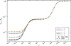Fig. C.1 Optical depth variations of normalised source functions for 1 ↔ 3 line of a three-level hydrogen atom. We compare FNLTE results (coloured lines) for various frequencies x = 0, 1, 2, 3, 4 with PRD reference solutions (black open circle) computed using the MALI-PRD method of Paletou (1995). The black dashed line shows the CRD solution computed using MALI-CRD method.

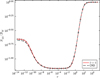Fig. C.2 Optical depth variations of normalised source functions for 2 ↔ 3 line of a three-level hydrogen atom. We compare FNLTE results (red line) with PRD reference solutions (black open circle) computed using the MALI-PRD method of Paletou (1995). The black dashed line shows the CRD solution computed using MALI-CRD method.

The combination of Eqs. (40), (C.2) then allows us to compare the results given by our FNLTE multi-level code with the reference results calculated using the MALI-PRD method developed by Paletou (1995). The results are shown in Fig. C.1 for the 1 ↔ 3 line and in Fig. C.2 for 2 ↔ 3 line. We do not show the results for 1 ↔ 2 line for the same reasons explained in Sect. 5.3. Finally, we see that the expected results are very well reproduced, with a mean relative error between the two solutions equal, for 1 ↔ 2, 1 ↔ 3 and 2 ↔ 3 lines respectively, to about 0.22%, 0.37% and 0.34%.

References

All Figures

Fig. 1 Frequency variation of normalised source function S12 of 1 ↔ 2 line at different optical depths τ for a two-level atom. Horizontal dashed black lines show CRD solutions for τ = 0, 1, 10, 100, 103, 104. We compare FNLTE results (coloured lines) with Hummer’s PRD results (black open circle). CRD and PRD solutions were computed using the ALI and FBF methods, respectively. Clearly, we accurately recover the results presented by Hummer (1969) and PSP23.

In the text

	Fig. 2 Optical depth variations of normalised source functions for each line of a three-level hydrogen atom in CRD. Our three-level FNLTE code (coloured lines) accurately reproduces reference solutions (open black circle) computed with MALI-CRD.
In the text

Fig. 3 Optical depth variations of normalised source functions for the 1 ↔ 3 line of a three-level hydrogen atom in the frame of XRD approximation. We compare FNLTE results (coloured lines) for various frequencies x = 0, 1, 2, 3, 4 with XRD reference solutions (open black circle) computed using the MALI-XRD method of Sampoorna et al. (2013). The dashed black line shows the CRD solution computed using the MALI-CRD method.

In the text

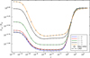	Fig. 4 Same as Fig. 3, but for 2 ↔ 3 line.
In the text

	Fig. 5 Optical depth variations of normalised source functions for 1 ↔ 3 line of a three-bound-level hydrogen atom. It shows FNLTE results (coloured lines) obtained for various frequencies: x = 0, 1, 2, 3, 4. The dashed black line represents the MALI-CRD solution.
In the text

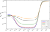	Fig. 6 Same as Fig. 5, but for 2 ↔ 3 line.
In the text

	Fig. 7 Frequency variations of ρ23 ratio for 2 ↔ 3 line of a three-bound-level hydrogen atom. We show the XRD (left plot) and FNLTE (right plot) results obtained for different optical depths: τ = 10−12, 10−10, 10−8, 10−5, 1.
In the text

	Fig. 8 Normalised atomic velocities variations of f3 velocity distribution of the second excited level of a three-bound-level hydrogen atom. Results (coloured lines) were obtained for different optical depths: τ31 = 0.5, 1, 10, 102, 108, 5 · 108, 1012. The dashed black line shows the Maxwellian limit f3(u) = fM(u).
In the text

	Fig. C.1 Optical depth variations of normalised source functions for 1 ↔ 3 line of a three-level hydrogen atom. We compare FNLTE results (coloured lines) for various frequencies x = 0, 1, 2, 3, 4 with PRD reference solutions (black open circle) computed using the MALI-PRD method of Paletou (1995). The black dashed line shows the CRD solution computed using MALI-CRD method.
In the text

	Fig. C.2 Optical depth variations of normalised source functions for 2 ↔ 3 line of a three-level hydrogen atom. We compare FNLTE results (red line) with PRD reference solutions (black open circle) computed using the MALI-PRD method of Paletou (1995). The black dashed line shows the CRD solution computed using MALI-CRD method.
In the text

References

- Avrett, E. H. 1968, in Resonance Lines in Astrophysics, eds. R. G. Athay, J. Mathis, & A. Skumanich (Boulder: National Center for Atmospheric Research), 27 [Google Scholar]
- Gray, M. 2012, Maser Sources in Astrophysics, 50 (Cambridge University Press) [Google Scholar]
- Heinzel, P., Gouttebroze, P., & Vial, J.-C. 1987, A&A, 183, 351 [NASA ADS] [Google Scholar]
- Hubeny, I. 1981, A&A, 100, 314 [Google Scholar]
- Hubeny, I. 1982, JQSRT, 27, 593 [Google Scholar]
- Hubeny, I. 1985, Bull. Astron. Inst. Czech., 36, 1 [Google Scholar]
- Hubeny, I. 2003, Stellar Atmos. Model., 288, 17 [Google Scholar]
- Hubeny, I., & Cooper, J. 1986, ApJ, 305, 852 [NASA ADS] [CrossRef] [Google Scholar]
- Hubeny, I., & Lites, B. W. 1995, ApJ, 455, 376 [NASA ADS] [CrossRef] [Google Scholar]
- Hubeny, I., & Mihalas, D. 2014, Theory of Stellar Atmospheres: An Introduction to Astrophysical Non-equilibrium Quantitative Spectroscopic Analysis, 26 (Princeton University Press) [Google Scholar]
- Hubeny, I., & Oxenius, J. 1987, JQSRT, 37, 65 [Google Scholar]
- Hubeny, I., Oxenius, J., & Simonneau, E. 1983a, JQSRT, 29, 477 [Google Scholar]
- Hubeny, I., Oxenius, J., & Simonneau, E. 1983b, JQSRT, 29, 495 [Google Scholar]
- Hummer, D. G. 1962, MNRAS, 125, 21 [Google Scholar]
- Hummer, D. G. 1969, MNRAS, 145, 95 [NASA ADS] [CrossRef] [Google Scholar]
- Lagache, T., Sampoorna, M., & Paletou, F. 2025, RAS Tech. Instrum., rzaf023 [Google Scholar]
- Milkey, R. W., Shine, R. A., & Mihalas, D. 1975, ApJ, 199, 718 [NASA ADS] [CrossRef] [Google Scholar]
- Oxenius, J. 1965, JQSRT, 5, 771 [Google Scholar]
- Oxenius, J. 1986, Kinetic Theory of Particles and Photons: Theoretical Foundations of Non-LTE Plasma Spectroscopy (Berlin: Springer) [Google Scholar]
- Paletou, F. 1995, A&A, 302, 587 [NASA ADS] [Google Scholar]
- Paletou, F., & Auer, L. H. 1995, A&A, 297, 771 [NASA ADS] [Google Scholar]
- Paletou, F., & Lagache, T. 2025, https://hal.science/hal-05051883 [Google Scholar]
- Paletou, F., & Léger, L. 2007, JQSRT, 103, 57 [Google Scholar]
- Paletou, F., & Peymirat, C. 2021, A&A, 649, A165 [NASA ADS] [CrossRef] [EDP Sciences] [Google Scholar]
- Paletou, F., Sampoorna, M., & Peymirat, C. 2023, A&A, 671, A93 [NASA ADS] [CrossRef] [EDP Sciences] [Google Scholar]
- Rybicki, G. B., & Hummer, D. G. 1991, A&A, 245, 171 [NASA ADS] [Google Scholar]
- Sampoorna, M., Nagendra, K. N., & Stenflo, J. O. 2013, ApJ, 770, 92 [Google Scholar]
- Sampoorna, M., Paletou, F., Bommier, V., & Lagache, T. 2024, A&A, 690, A213 [NASA ADS] [CrossRef] [EDP Sciences] [Google Scholar]
- Uitenbroek, H. 1989, A&A, 213, 360 [NASA ADS] [Google Scholar]
The atomic emission profile was previously written, η (see e.g. Oxenius 1986 or HOSI and HOSII), but we renamed it β in order to avoid any confusion with the emissivity.
Velocity-changing collisions cannot populate a given level i from a level j. However, they change the velocity of the atom inducing a transition from one state (position and velocity) to another in phase space. These collisions therefore populate a level by creating or destroying particles in phase space.