| Issue |
A&A
Volume 688, August 2024
|
|
|---|---|---|
| Article Number | A137 | |
| Number of page(s) | 10 | |
| Section | The Sun and the Heliosphere | |
| DOI | https://doi.org/10.1051/0004-6361/202449435 | |
| Published online | 12 August 2024 | |
Diagnostic potential of wavelength-integrated scattering polarisation in the solar He II Ly-α line
1
Istituto ricerche solari Aldo e Cele Daccò (IRSOL), Faculty of Informatics, Università della Svizzera italiana (USI), 6605 Locarno, Switzerland
e-mail: fabio.riva@irsol.usi.ch
2
Euler Institute, Università della Svizzera italiana (USI), 6900 Lugano, Switzerland
3
Institut für Sonnenphysik (KIS), 79110 Freiburg i. Br., Germany
Received:
31
January
2024
Accepted:
19
April
2024
Aims. The main goal of this work is to study the potential of the He II Ly-α wavelength-integrated scattering polarisation for probing the magnetism of the solar upper chromosphere. Meanwhile, the suitability of different modelling approximations is investigated.
Methods. Radiative transfer calculations are performed in semi-empirical 1D solar atmospheres, out of local thermodynamic equilibrium, considering a two-term atomic model and accounting for the Hanle, Zeeman, and magneto-optical effects. The problem is suitably linearised and discretised, and the resulting numerical system is solved with a matrix-free iterative method. The results obtained by modelling scattering processes with three different descriptions, namely in the limit of complete frequency redistribution (CRD), and accounting for partial frequency redistribution (PRD) effects under the angle-averaged (AA) approximation and in the general angle-dependent (AD) formulation, are compared.
Results. The synthetic Stokes profiles resulting from CRD, PRD–AA, and PRD–AD calculations show a very good agreement in the line core, while some differences are observed in Q/I outside this spectral region. Moreover, the precise structure of the atmospheric model does not noticeably affect the line-core profiles, but it strongly impacts the Q/I signals outside the line core. As most of the He II Ly-α photons originate in the core region, it turns out that wavelength-integrated linear polarisation signals are almost insensitive to both the scattering description and the atmospheric model. Appreciable wavelength-integrated Ū/Ī signals, showing observable sensitivity to horizontal magnetic fields in the 0–1000 G range, are also found, particularly near the limb. While the integration time required to detect magnetic fields in the quiet chromosphere with this line is too long for sounding-rocket missions, magnetic fields corresponding to typical plage areas would produce detectable signals, especially near the limb.
Conclusions. These results, to be confirmed by 3D calculations including the impact of horizontal inhomogeneities and bulk velocity gradients, show that filter polarimetry in the He II Ly-α line has a promising potential for chromospheric magnetic-field diagnostics. In near-limb plage regions, this could already be assessed through sounding-rocket experiments.
Key words: polarization / radiative transfer / scattering / methods: numerical / Sun: atmosphere / Sun: chromosphere
© The Authors 2024
 Open Access article, published by EDP Sciences, under the terms of the Creative Commons Attribution License (https://creativecommons.org/licenses/by/4.0), which permits unrestricted use, distribution, and reproduction in any medium, provided the original work is properly cited.
This article is published in open access under the Subscribe to Open model. Subscribe to A&A to support open access publication.
1. Introduction
The dynamics of the outer layers of the solar atmosphere is largely governed by the presence of magnetic fields, which, however, are notoriously hard to measure. The most promising state-of-the-art remote-sensing approach to overcome this difficulty and explore the magnetism of the solar upper chromosphere and transition region is the interpretation of the polarisation signals produced by both the Zeeman effect and scattering processes in strong UV resonance lines, such as Mg II h&k, H I Ly-α, or He II Ly-α (e.g. Trujillo Bueno & del Pino Alemán 2022). Unfortunately, the Zeeman effect is not very effective at short wavelengths and in hot plasmas. Thus, the signals produced by the weak magnetic fields of the quiet solar chromosphere through this mechanism can hardly be detected in far and extreme UV lines. On the other hand, all the aforementioned resonance lines show measurable linear-scattering-polarisation signals, with an interesting magnetic sensitivity via the combined action of the Hanle and magneto-optical (MO) effects (see e.g. the review by Trujillo Bueno et al. 2017).
Thanks to its sensitivity to chromospheric magnetic fields, the H I Ly-α line at 1216 Å has attracted increasing attention during the last few years. Modelling scattering processes within the limit of complete frequency redistribution (CRD) and neglecting J-state interference, Trujillo Bueno et al. (2011) showed that the line-core-scattering-polarisation signal is sensitive to, via the Hanle effect, the presence of magnetic fields between 10 G and 100 G in the upper chromosphere. Štěpán et al. (2012, 2015) extended the investigation of the Hanle sensitivity of the H I Ly-α line by considering realistic 2D and 3D atmospheric models resulting from a state-of-the-art radiation magneto-hydrodynamic simulation. A very interesting outcome of these investigations is that the centre-to-limb variation (CLV) of the spatially averaged line-core Q/I signal is qualitatively similar to that found considering semi-empirical 1D atmospheric models. Moreover, Belluzzi et al. (2012) showed that the joint action of partial frequency redistribution (PRD) and J-state interference effects produces conspicuous wing-scattering-polarisation signals, which are very sensitive to the chromospheric thermal structure. These results motivated the development of the Chromospheric Lyman-Alpha Spectro-Polarimeter (CLASP) sounding-rocket experiment (Kobayashi et al. 2012; Kano et al. 2012), which paved the way to the observation of the intensity and linear polarisation of the solar H I Ly-α line. The CLASP data showed a remarkably good qualitative agreement with the theoretical predictions (Kano et al. 2017) and have been exploited to obtain new constraints on the magnetisation and the degree of corrugation of the chromosphere-corona transition region (Trujillo Bueno et al. 2018). More recently, Alsina Ballester et al. (2019, 2023) proved that the wavelength-integrated linear polarisation signals of this line are strongly sensitive to magnetic fields of strengths of about 50 G in the middle–upper chromosphere via MO effects.
By contrast, fewer investigations have been dedicated to the scattering-polarisation signals of the He II Ly-α line at 304 Å, and especially to its magnetic sensitivity. This is for two reasons. First, the He II Ly-α line is much less sensitive to the Hanle effect than the H I Ly-α line. Indeed, having a much larger Einstein coefficient for spontaneous emission, the Hanle critical field of the He II Ly-α line is BH ≈ 850 G, while the H I Ly-α line has BH ≈ 53 G. By applying the CRD limit, Trujillo Bueno et al. (2012) confirmed that the He II Ly-α line-core Q/I signal is nearly immune to magnetic fields weaker than 100 G; they thus proposed to use it as a reference signal for a differential Hanle effect technique. Second, although the He II Ly-α line shows large fractional linear polarisation signals, the number of emitted photons in this line is significantly smaller than in H I Ly-α (e.g. Fontenla et al. 1993) and the required exposure time to reach any given polarimetric sensitivity is thus much longer (e.g. Trujillo Bueno & del Pino Alemán 2022).
The scattering-polarisation signals of the He II Ly-α line in unmagnetised atmospheres were further explored in Belluzzi et al. (2012), showing that the joint action of PRD and J-state interference effects produces complex scattering-polarisation Q/I profiles with sharp peaks of large amplitude outside the line-core region. Although these peaks are largely insensitive to the Hanle effect, in principle they could be impacted by magnetic fields through the action of MO effects (e.g. Alsina Ballester et al. 2016; del Pino Alemán et al. 2016). This potential yet unexplored magnetic sensitivity of the He II Ly-α line motivates the work detailed in the present paper. Moreover, we note that for computational simplicity the PRD calculations of Belluzzi et al. (2012) were performed within the angle-averaged (AA) approximation (e.g. Mihalas 1978; Leenaarts et al. 2012; Sampoorna et al. 2017; Alsina Ballester et al. 2017). The suitability of such an approximation in the modelling of He II Ly-α line polarisation signals has yet to be proven.
Motivated by the studies of Trujillo Bueno et al. (2012) and Belluzzi et al. (2012), the main goal of this work is to investigate the potential of He II Ly-α wavelength-integrated scattering polarisation for probing the magnetism of the upper solar chromosphere. Concurrently, we aim to assess the suitability of the CRD and PRD–AA approximations for modelling the polarisation profiles and the wavelength-integrated polarisation signals of this line. This is done through a comparison with general angle-dependent (AD) PRD calculations, which are more accurate, but they also imply a significantly higher computational cost.
The present article is organised as follows. Section 2 details the considered non-equilibrium transfer problem for polarised radiation, as well as its linearisation, discretisation, and algebraic formulation. Section 3 presents the adopted numerical solution strategy and the numerical setup. In Sect. 4, we report and analyse the synthetic emergent Stokes profiles of the He II Ly-α line, comparing CRD, PRD–AA, and PRD–AD calculations and investigating the impact that the magnetic field and the atmospheric parameters have on the numerical results. Finally, Sect. 5 discusses the main results and their implications and provides some final considerations.
2. Formulation of the problem
Aiming to model the scattering-polarisation signal of the He II Ly-α line at 304 Å, we solved the non-equilibrium transfer problem for polarised radiation in 1D models of the solar atmosphere. To correctly model this signal, a two-term atomic model, which includes quantum interference between different fine-structure (FS) levels of the same term (J-state interference, see Landi Degl’Innocenti & Landolfi 2004), has to be considered (Belluzzi et al. 2012). Scattering processes are modelled considering three different descriptions of increasing computational complexity, namely in the CRD limit, and including PRD effects in the AA approximation, and in their general AD formulation. We also consider the impact of magnetic fields of arbitrary strength and orientation, accounting for the Hanle, Zeeman, and MO effects. The theoretical framework is presented in the following sub-sections.
2.1. Two-term atomic model
The He II Ly-α line results from two distinct FS transitions between the ground level of ionised helium 1s 2S1/2 and the excited levels  and
and  . These two FS components are separated by 5 mÅ only, and they are thus completely blended. To take into account both these transitions and the J-state interference between the two upper levels, we consider a two-term 2S–2P o atomic model. Noticing that the lower level cannot carry atomic alignment (see Landi Degl’Innocenti & Landolfi 2004) and has a very long lifetime, we can assume that it is unpolarised and infinitely sharp. Neglecting stimulated emission, which is generally a good assumption in the solar atmosphere, the statistical equilibrium equations for a two-term atom with unpolarized and infinitely-sharp lower term have an analytic solution. Thus, the scattering contribution to the line emissivity can be expressed through the redistribution matrix formalism, which is a very convenient formulation for modelling PRD effects. In this work, we used the redistribution matrix for the aforementioned atomic system as derived by Bommier (2017, see Sect. 2.4). For the energies of the upper levels
  and
and  , relative to the ground state, we considered Eu = 329 179.29 cm−1 and Eu = 329 185.15 cm−1, respectively; while, for the Einstein coefficient for spontaneous emission from upper to lower term, we used Aul = 1.0029 × 10¹⁰ s−1, as given by the NIST database (Kramida et al. 2023). The splitting of the magnetic sub-levels in the presence of a magnetic field was calculated considering the Paschen-Back effect1. We finally note that only the transition from the upper level
  contributes to the emergent linear-scattering polarisation (Trujillo Bueno et al. 2011).
2.2. Semi-empirical 1D atmospheric models
The calculations presented in the following were obtained with the plane-parallel semi-empirical 1D models of Fontenla et al. (1993, hereafter FAL models), making use of the microturbulent velocities as determined in Fontenla et al. (1991). In particular, we considered three quiet-Sun atmospheric models, representing a faint inter-network region (FAL-A), a bright network region (FAL-F), and an average region (FAL-C), as well as a model that mimics a plage area (FAL-P), that is, a region that appears particularly bright in the chromospheric Hα line, typically found next to active solar regions. Despite their simplicity, these atmospheric models are realistic enough to assess the potential of He II Ly-α wavelength-integrated scattering polarisation for investigating chromospheric magnetic fields.
2.3. Radiative-transfer equation
The intensity and polarisation of a beam of radiation are fully described by the Stokes parameters I, Q, U, and V, hereafter gathered in the Stokes vector I = (I, Q, U, V)T ∈ ℝ4. Considering a Cartesian reference system with the z-axis (quantisation axis for total angular momentum) directed along the vertical, the transfer of partially polarised radiation is described by the following differential equation:

where the vector Ω = (θ, χ)∈[0, π]×[0, 2π) and the scalar ν specify the direction and the frequency, respectively, of the considered radiation beam. The inclination θ is measured with respect to the z-axis and corresponds to the heliocentric angle (generally specified by μ = cos θ ∈ [ − 1, 1]) of the observed point. The azimuth χ is measured from the x-axis anti-clockwise for an observer at positive z. The propagation matrix K ∈ ℝ4 × 4 quantifies how the medium attenuates the specific intensity for all polarisation states (absorption) and how it differentially absorbs (dichroism) and couples (MO effects) the different Stokes parameters. The emission vector ε ∈ ℝ4 describes the polarised radiation emitted by the solar plasma.
In the following, we consider the contributions to K and ε due to both line and continuum processes. These contributions, labelled with the superscripts ℓ and c, respectively, simply sum up. Moreover, both εℓ and εc can in turn be written as the sum of two terms, describing the contributions from scattering (label “sc”) and thermal (label “th”) processes, respectively. Hence, we have

and
The explicit expressions for Kc and Kℓ are given by Landi Degl’Innocenti & Landolfi (2004), while we refer to the work of Alsina Ballester et al. (2022) for εc, th, εc, sc, and εℓ, th. The line-scattering contribution to emissivity, εℓ, sc, is described in the following section.
2.4. Line scattering emissivity
Using the redistribution matrix formalism and following the convention that primed and unprimed quantities refer to the incident and scattered radiation, respectively, the line scattering term can be written through the following scattering integral:

where the factor kM is the wavelength-integrated absorption coefficient (e.g. Alsina Ballester et al. 2022) and R ∈ ℝ4 × 4 is the redistribution matrix for the considered two-term atomic model (see Bommier 2017). We recall that R encodes the statistical equilibrium (SE) equations, which determine the state of the atomic system.
The redistribution matrix can be expressed as the sum of two terms, R = RII + RIII, which describe scattering processes that are coherent (II) and completely incoherent (III) in the atomic reference frame. In the observer’s frame, we consider both the general AD expression of RII, as well as its AA approximation. As far as RIII is concerned, we considered its simplified expression under the assumption of CRD in the observer’s frame (see e.g. Bommier 1997; Sampoorna et al. 2017; Alsina Ballester et al. 2017; Riva et al. 2023). For conciseness, we refer to the work of Alsina Ballester et al. (2022) for the analytical expressions of RII in the observer’s frame (both AA and AD) as well as for the expression of RIII, under the aforementioned assumption of CRD in the observer’s frame. Moreover, we note that the limit of CRD is obtained by artificially increasing the rate of elastic collisions in the branching ratios of RII and RIII so that the contribution of the former vanishes (see Alsina Ballester et al. 2022). In this respect, we recall that the considered redistribution matrix does not account for the depolarising effect of elastic collisions with neutral perturbers, because the SE equations for a two-term atom in the presence of magnetic fields cannot be solved analytically when such an effect is included (see Bommier 2017 for more details). Noticing that Alsina Ballester et al. (2021) verified that this effect can be safely ignored for the Na I D lines, we can argue that the same conclusion also holds for the He II Ly-α line, which forms significantly higher in the solar atmosphere.
2.5. Linearisation, discretisation, and algebraic formulation
The radiative transfer (RT) problem consists of finding a self-consistent solution of the RT equation for the radiation field I and of the SE equations for the atomic system, whose state determines K and ε. In general, the problem is integro-differential, non-local, and non-linear. In our formulation, based on the redistribution matrix formalism, the non-linearity lies in the dependence of both K and ε on the coefficient kM. This coefficient is proportional to the population of the lower term, which in turn non-linearly depends on I through the SE equations (see e.g. Landi Degl’Innocenti & Landolfi 2004). However, the RT problem can be suitably linearised by fixing the coefficient kM a priori, which corresponds to assuming a fixed lower term population (see e.g. Belluzzi & Trujillo Bueno 2014; Sampoorna et al. 2017; Alsina Ballester et al. 2017; Janett et al. 2021; Benedusi et al. 2021, 2022). This assumption makes the propagation matrix K independent of I, whereas ε only depends on I linearly. In this case, the whole problem consists of finding a self-consistent solution of Eqs. (1)–(3), and it is linear in I.
To numerically solve the resulting linearised RT problem, we first need to discretise the continuous variables z, Ω, and ν. The spatial discretisation is done by using Nr unevenly spaced grid nodes. The angular grid, which samples the unit sphere with NΩ angular nodes, usually depends on the quadrature chosen to evaluate the angular integral in Eq. (3) (see Sect. 3.1). Finally, we consider a finite spectral interval [νmin, νmax] for ν, discretised with Nν unevenly spaced nodes. More details on the numerical parameters used for the present work are given in Sect. 3.4.
The discretised radiation field and emissivity vectors are thus represented by I ∈ ℝN and ε ∈ ℝN, with N = 4NrNνNΩ being the total number of degrees of freedom. Hence, we can express the transfer equation, Eq. (1), and the calculation of the emission coefficient, Eq. (2), as


respectively. Here, the transfer operator Λ ∈ ℝN × N and the scattering operator Σ ∈ ℝN × N are linear, the vector t ∈ ℝN represents the radiation transmitted from the boundaries, while εth ∈ ℝN represents the thermal contributions to the emissivity. The evaluation of the term Λε + t is commonly known as a formal solution and consists of the numerical solution of Eq. (1) for I, provided there are ε, K, and appropriate boundary conditions. The term ΣI corresponds to the numerical evaluation of the scattering contribution to the emission vector, given I. This requires approximating the integral in Eq. (3) via suitable quadrature rules (see Sect. 3.1). Equations (4) and (5) can then be combined into a matrix equation of the form Ax = b, namely
with Id ∈ ℝN × N being the identity matrix (see e.g. Janett et al. 2021; Benedusi et al. 2022).
3. Methods and setting
We now detail the numerical methods employed to solve Eq. (6) and the physical and numerical parameters used in the calculations.
3.1. Angular and spectral quadratures
The numerical integration of Eq. (3) requires a proper choice of quadrature rules. For the angular integral, we resorted on a tensor product of a trapezoidal quadrature in the azimuthal interval [0, 2π) for χ and two Gauss–Legendre quadratures, one in each inclination subinterval ( − 1, 0) and (0, 1) for μ = cos(θ). For the integral in ν′, we selected a set of spectral points distributed ad hoc to approximately follow the shape of the redistribution matrix R. More precisely, we used a Gauss–Hermite quadrature rule in spectral regions where R is similar to a Gaussian function, while we used a Gauss–Legendre quadrature rule in the rest of the parameter domain.
3.2. Formal solution
For a better agreement with the results by Belluzzi et al. (2012), we applied the DELOPAR formal solver to evaluate the Λ operator in Eq. (6) (for details, see Trujillo Bueno 2003; Janett et al. 2017, 2018; Janett & Paganini 2018) using a trapezoidal quadrature for the conversion to optical depth. We note that the use of the L-stable DELO-linear method only affects the amplitude of the emergent Stokes profiles, but it leads to the same general conclusions.
3.3. Iterative solver
The whole transfer problem has been recast in the linear system given by Eq. (6), for which we have to find a solution. Given the size of the system, with N ∼ 106 (see Sect. 3.4), the use of direct matrix inversion solvers is definitely unfeasible. Thus, the application of an iterative method was preferred. Moreover, it is also too expensive to explicitly assemble the dense operator Id − ΛΣ in Eq. (6). Therefore, the action of the operator Id − ΛΣ was encoded in a routine, and an iterative method was applied in a matrix-free context.
In this work, we applied a Krylov solver, namely the generalised-minimal-residual (GMRES) method, which proved to be highly effective in terms of convergence rate and time to solution for this kind of problem (Benedusi et al. 2021, 2022, 2023). We additionally exploited the innovative approach to designing efficient physics-based preconditioners and initial guesses extensively described in Janett et al. (2024), and we monitored the convergence of the GMRES iterative method by considering the relative residual
taking res < tol = 10−9 as a stopping criterion. In the calculations presented in this paper, both CRD- and PRD–AA-based preconditioners have a noticeable impact, ensuring a solution of the problem in 4–8 iterations. Moreover, the inclusion of polarisation in the preconditioner has little impact (with respect to the unpolarised version), and it is thus neglected.
3.4. Physical and numerical parameters
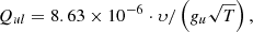
The lower term population (i.e. the population of the ground level of ionised helium) was provided by the FAL atmospheric models (Fontenla et al. 1993). The RH code by Uitenbroek (2001) was used to calculate the continuum total opacity, scattering opacity, and thermal emissivity. Moreover, it provided the rate of elastic collisions, calculated including the contribution from the Van der Waals interaction with neutral hydrogen and helium atoms (Unsöld 1955), as well as the damping parameter. The rate of inelastic de-exciting collisions was evaluated as Cul = NeQul, with Ne being the electron density and
where gu = 6 is the degeneracy of the upper term, T is the local temperature, and υ (which depends on T) is taken from Janev et al. (1987). For the formal solution, we assumed the following boundary conditions:
![$$ \begin{aligned}&I(z_{\min },\theta ,\chi ,\nu ) = B_P,\qquad \qquad \mathrm{for}~\theta \in [0, \pi /2), \forall \chi , \forall \nu ,\\&I(z_{\max },\theta ,\chi ,\nu ) = 0,\qquad \qquad \mathrm{for}~\theta \in (\pi /2, \pi ], \forall \chi , \forall \nu , \end{aligned} $$](/articles/aa/full_html/2024/08/aa49435-24/aa49435-24-eq16.gif)
where BP is the line-centre-frequency Planck function at the local temperature.
The wavelength interval [λmin,λmax] = [303.01 Å, 304.55 Å] was discretised with Nν = 141 frequency nodes, approximately uniformly spaced in the line core and logarithmically distributed in the wings. The spatial grid was provided by the considered semi-empirical 1D atmospheric models. However, since the He II Ly-α line forms in a very narrow region in the outermost layers of the solar chromosphere (e.g. Trujillo Bueno et al. 2012; Belluzzi et al. 2012), we decided to cut out the layers below zmin = 1375, 1475, 1475, and 1495 km for the FAL-A, FAL-C, FAL-F, and FAL-P models, respectively, as their contribution to the emergent radiation field is negligible2. Conversely, we doubled the spatial resolution in the uppermost layers by introducing a new set of grid points equidistant to each pair of adjacent original points and by linearly interpolating the input variables to the new grid. This resulted in 61–76 unevenly distributed spatial nodes, depending on the considered atmospheric model. For the angular discretisation, we used two six-node Gauss–Legendre grids for the inclination and a nine-node grid for the azimuth.
4. Results
The physical problem discussed in Sect. 2 and discretised as outlined in Sect. 3 was implemented as a MATLAB (MATLAB 2023) routine and solved with the MATLAB gmres solver. In this section, we present the numerical results obtained for the He II Ly-α line with two main goals. First, we aim to assess the suitability of the CRD and PRD–AA modellings through comparisons with the general PRD–AD calculations, both in the absence and presence of magnetic fields. Second, we investigate the potential of the wavelength-integrated scattering-polarisation signal of this line for probing the magnetism of the solar chromosphere.
4.1. Impact of PRD–AD effects
The impact of the PRD–AD treatment on the emergent Stokes profiles is first analysed considering the FAL-C atmospheric model and two lines of sight (LOSs), with μ = 0.1 and μ = 0.9. Figures 1 and 2 detail the synthetic emergent Stokes profiles in the absence and in the presence of a magnetic field, respectively. For the latter case, as an example of interest, we considered a uniform horizontal (θB = π/2 and χB = 0) magnetic field of strength B = 100 G. In the unmagnetic case, the U/I and V/I profiles vanish and are consequently not shown. In addition, as the I profile is not affected by magnetic fields of practical interest, it is only displayed for the unmagnetic case in Fig. 1.
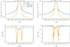 |
Fig. 1. Stokes I (top panels) and Q/I (bottom panels) profiles for the He II Ly-α line as a function of wavelength. The results are obtained with the unmagnetised FAL-C atmospheric model and for two LOSs, near the limb (μ = 0.1, left panels) and near the disc centre (μ = 0.9, right panels), respectively. Blue, red, and yellow lines correspond to CRD, PRD–AA, and PRD–AD calculations, respectively. The intensity is in units of number of photons per unit of surface, time, wavelength, and solid angle. The intensity profiles for PRD–AA and PRD–AD calculations overlap. |
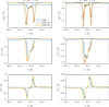 |
Fig. 2. Stokes Q/I (top panels), U/I (middle panels), and V/I (bottom panels) profiles for the He II Ly-α line as a function of wavelength. The results are obtained with the FAL-C atmospheric model, with a uniform horizontal (θB = π/2 and χB = 0) magnetic field of 100 G, and for two LOSs, near the limb (μ = 0.1, left panels) and near the disc centre (μ = 0.9, right panels), respectively. Blue, red, and yellow lines correspond to CRD, PRD–AA, and PRD–AD calculations, respectively. The unmagnetic CRD and PRD–AD cases are given for reference as dash-dotted and solid black lines, respectively. |
In the core of the line, we find a good agreement between the CRD, PRD–AA, and PRD–AD calculations for all Stokes profiles, both in the absence and in the presence of magnetic fields. Reasonably, the CRD modelling is, however, not able to reproduce the large peaks outside the line-core region of the Q/I profiles. For these peaks, noticeable discrepancies are found between PRD–AA and PRD–AD calculations for a LOS near the disc centre (μ = 0.9). This is not true near the limb (μ = 0.1), where PRD–AA and PRD–AD calculations show excellent agreement.
We note that the Stokes Q/I, U/I, and V/I profiles obtained at μ = 0.1 are very similar to those obtained at μ = 0.3, both in the presence and in the absence of magnetic fields. Thanks to this coincidence, the profiles calculated at μ = 0.1 in this work can be quantitatively compared to results for μ = 0.3 reported elsewhere in the literature. The remarkably good agreement between the profiles of Fig. 1 and those of Fig. 3 of Belluzzi et al. (2012) proves the robustness of our results, considering that the calculations of the two works were carried out applying completely different solution strategies. Moreover, we recall that the results of Belluzzi et al. (2012) were obtained applying the redistribution matrix of Belluzzi & Trujillo Bueno (2014), which differs from that of Bommier (2017) in the RIII term3.
Figure 2 shows that, as expected, the Q/I signal is barely sensitive to the Hanle effect for the considered magnetic field of 100 G (compare the colour and the black lines). Moreover, because of the reduced effectiveness of the Zeeman effect at these wavelengths, the circular polarization signal is much weaker than the linear ones. On the other hand, a significant Hanle signal appears in U/I, particularly near the limb (see the central left panel). For μ = 0.1, we have Q/I ≃ −1% and U/I ≃ −0.3% at the line centre. These amplitudes slightly underestimate the CRD results shown in the left panel of Fig. 5 of Trujillo Bueno et al. (2012). In addition, the MO effects seem to play a marginal role for the considered cases. To confirm this, we performed the same calculations by setting the MO term of the propagation matrix to zero (see Alsina Ballester et al. 2017), obtaining almost overlapping emergent Q/I and U/I signals. The same conclusion applies when repeating this study with a stronger horizontal magnetic field of 500 G. For the sake of completeness, we also carried out calculations analogous to Fig. 2, but for vertical magnetic fields (not shown here for conciseness). For magnetic-field strengths typical of the quiet solar chromosphere, the Q/I signals did not display any noticeable variation with respect to the unmagnetic case, while the U/I signals were extremely weak and therefore of reduced diagnostic interest.
A striking difference between the CRD and PRD results of Figs. 1 and 2 appears in the I, Q/I, and U/I profiles far away from the line centre. In particular, the amplitude of the fractional polarisation signals at distances larger than 0.1 Å from the line centre is much larger for CRD than for PRD calculations. A detailed investigation of these results (not reported here for conciseness) revealed that this different behaviour is not due to continuum contributions, which in this spectral region are extremely low. The difference is rather due to the strong redistribution effects resulting from the slowly decreasing wings of the Voigt emission profile entering the RIII redistribution matrix describing the CRD limit, combined with the very large and sharp emission peak of this line (moving away from the line centre, the intensity decreases by more than four orders of magnitude in about 0.1 Å)4. This leads to Stokes profiles that are much broader for the CRD than for the PRD case.
4.2. Sensitivity of Stokes profiles to the atmospheric model
To analyse the sensitivity of the He II Ly-α emergent Stokes profiles to atmospheric conditions, we considered the four plane-parallel semi-empirical 1D FAL-A, FAL-C, FAL-F, and FAL-P atmospheric models, and we solved the RT problem in the presence of a uniform horizontal (θB = π/2 and χB = 0) magnetic field of 100 G. Figure 3 shows the emergent Q/I, U/I, and V/I profiles for the aforementioned atmospheric models and a LOS with μ = 0.1 and χ = 0. We found a very good agreement in the line core of the Q/I profile. On the other hand, some relevant differences appear in the peaks just outside the line-core region. Moreover, the U/I and V/I signals almost overlap for all the considered atmospheric models. We note that, although we only showed the μ = 0.1 case, good agreement was found for all LOSs. We also note that, although the present Q/I profiles were obtained in a magnetised atmosphere, these are in excellent qualitative agreement with those in Fig. 4 of Belluzzi et al. (2012) for a LOS with μ = 0.3.
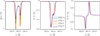 |
Fig. 3. Stokes Q/I (left panel), U/I (middle panel), and V/I (right panel) profiles for the He II Ly-α line as a function of wavelength. The results are obtained performing PRD-AD calculations for a LOS near the limb (μ = 0.1 and χ = 0) and with a uniform horizontal (θB = π/2 and χB = 0) magnetic field of 100 G. Blue, red, yellow, and purple lines correspond to profiles obtained with the FAL-A, FAL-C, FAL-F, and FAL-P atmospheric models, respectively. |
4.3. Wavelength-integrated linear-polarisation signals
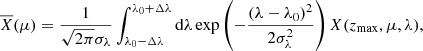
We now focus on the He II Ly-α linear polarisation signals obtained using narrow-band filters. Following Alsina Ballester et al. (2023), synthetic narrow-band signals can be obtained by integrating over wavelength the numerical emergent Stokes profiles, weighted by a Gaussian that mimics the action of a narrow-band filter:
where X = I, Q, U, λ0 = 303.784 Å is the He II Ly-α line-centre wavelength in vacuum, and σλ is the standard deviation of the Gaussian weighting function, which corresponds to a full width at half maximum (FWHM) of  (here, we do not consider the circular polarisation signal as its profile is antisymmetric, and thus
  vanishes). We note that the choice of FWHM affects the amplitude of the narrow-band signals
  ,
,  , and
, and  , but it does not impact the ratios
  and
and  and their dependency on μ. In addition, any choice with Δλ ≥ 0.5 Å has no impact on the results, because both the intensity and the scattering-polarisation signals quickly drop to zero when moving away from the line centre. Thus, in the calculations, we adopted a FWHM of 1 Å and used Δλ = 1 Å.
Figure 4 displays the CLV of the narrow-band  and
and  signals for LOSs with μ ∈ [0.1, 0.9], considering the FAL-C atmospheric model in the presence of uniform horizontal magnetic fields of strengths between 0 and 1000 G. For B ≤ 200 G, the amplitude of the
  and
and  signals increases from the disc centre to the limb for all the scattering descriptions, reaching a maximum close to μ = 0.2 and then slightly decreasing towards μ = 0.1. This behaviour is consistent with the similarity of the Q/I and U/I profiles obtained at μ = 0.1 and μ = 0.3, pointed out in Sect. 4.1. Moreover, the
  signal proves to be almost insensitive to magnetic-field strengths of B ≤ 50 G, while its amplitude decreases for 200 G ≥ B ≥ 50 G. Conversely, the amplitude of the
  signal increases almost linearly with B for all the considered inclinations. For B > 200 G, the amplitude of
  reaches a maximum near B = 500 G and then decreases for stronger magnetic fields. This behaviour of
  and
and  is due to the Hanle effect, which produces a rotation of the plane of linear polarisation and a depolarisation. Furthermore, we note that the
  signals become positive closer to the disc centre, with a larger amplitude for stronger magnetic fields. This is due to the forward-scattering Hanle effect (Trujillo Bueno et al. 2002). In general, we found a very good agreement between CRD, PRD–AA, and PRD–AD calculations, although the CRD description slightly underestimates the amplitude compared to the PRD case, in particular for μ < 0.5. Noticeably, the agreement between PRD–AA and PRD–AD calculations decreases near the disc centre for B ≥ 500 G.
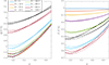 |
Fig. 4. Centre-to-limb variation of |


To investigate the dependence of the synthetic narrow-band signals on atmospheric parameters, in Fig. 5 we present  and
and  as a function of the strength of the horizontal magnetic field for the three different LOSs, μ = 0.1, 0.6, and 0.9, and for the four aforementioned FAL atmospheric models. The dependence of all signals on the considered atmospheric models is negligible. Moreover, the left panel of Fig. 5 shows that
  is almost flat for B < 50 G, while it reveals a slight Hanle depolarisation for stronger magnetic fields, which is in agreement with the results presented in Fig. 4. In addition, in the right panel of Fig. 5 we see that the amplitude of the appreciable
  signal increases almost linearly with B, which is also in agreement with the results in Fig. 4.
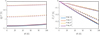 |
Fig. 5. Plots of |


5. Discussion and conclusions
In Sect. 4.3, we show that synthetic narrow-band signals of the He II Ly-α line are insensitive to the considered atmospheric models. At the same time, a study of the impact of bulk velocities on the He II Ly-α line (not reported here for conciseness) revealed that  and
and  are also insensitive to typical chromospheric plasma bulk velocities5. We also show that, although the Stokes profiles are nearly immune to MO effects,
  displays an almost linear dependence on B (via the Hanle effect) for magnetic strengths typical of the quiet solar chromosphere and that
  is almost insensitive to magnetic fields of strength weaker than 50 G. Consequently, since
  near the solar limb for a horizontal magnetic field of 100 G, He II Ly-α linear polarisation signals obtained using narrow-band filters may represent an interesting and novel capability to infer chromospheric magnetic fields, provided that a sufficient signal-to-noise ratio can be achieved.
It is thus important to assess the integration time, tint, necessary to be sensitive to chromospheric magnetic fields for a given instrument. In this respect, we applied Eq. (56) of Trujillo Bueno et al. (2017) considering the following: a near-limb LOS, for which  and
and  are maximal; a polarimetric sensitivity of 0.05%, which, in the present geometry, means a sensitivity to horizontal magnetic fields of about 10 G; an instrumental efficiency of 1%; a spatial resolution of 2 arcsec; a diameter of the telescope of 30 cm, similar to that of the instrument installed on the CLASP experiment (Kobayashi et al. 2012); and a FWHM of the narrow-band filter of 1 Å. Given these constraints, we found that the integration time necessary to be sensitive to horizontal chromospheric magnetic fields of 10 G is tint = 885, 447, 157, and 22 s for the atmospheric models FAL-A, FAL-C, FAL-F, and FAL-P, respectively. We note that, while
  and
and  are independent of the atmospheric model, tint is not, as the intensity signal, and thus the number of photons reaching the telescope, strongly depend on the atmospheric temperature structure.
Concerning quiet-solar conditions (i.e. models FAL-A, FAL-C, and FAL-F), the resulting tint are too large to be reached through sounding-rocket experiments. On the other hand, the integration time for the FAL-P model, which corresponds to a typical plage area, is realistic for present-day rockets (e.g. CLASP). Overall, valuable He II Ly-α polarisation signals could also be measured in quiet regions across the whole solar disc; this would be done via spacecraft missions, as these allow for considerably larger telescopes and longer exposure times than sounding-rocket experiments. Indeed, the integration time scales as tint ∝ 1/D2, with D being the diameter of the telescope. Thus, for a telescope with an aperture of, for example, 50 cm, we would have integration times that are shorter than those reported above by about a factor three, that is, 3–5 min for quiet solar conditions.
Another interesting outcome of the work is the very good agreement of wavelength-integrated He II Ly-α fractional linear polarisation signals obtained from CRD, PRD–AA, and PRD–AD calculations, especially for magnetic fields up to 200 G. This means that a complete PRD–AD description of scattering processes seems not to be strictly necessary to accurately model the impact of such magnetic fields on these signals. The CRD formulation could be enough. This would drastically reduce the computational cost of inferring magnetic fields from future He II Ly-α observations.
We remind the reader that the results in the present paper were obtained using a semi-empirical 1D model. However, the solar atmosphere is definitely not 1D, but it has large horizontal inhomogeneities as well as bulk velocities with strong gradients, which can strongly impact the amplitude and shape of scattering-polarisation signals (e.g. Manso Sainz & Trujillo Bueno 2011; Štěpán & Trujillo Bueno 2016; Jaume Bestard et al. 2021). This is particularly true in the upper chromosphere. Consequently, in the future it will be essential to assess the impact of these effects on the polarisation signals of the He II Ly-α line through full 3D RT calculations in state-of-the-art models of the solar atmosphere. The same 3D calculations, to be performed both in CRD (e.g. using the PORTA code of Štěpán & Trujillo Bueno 2013) and in PRD (e.g. using a code based on the solution strategy outlined in Benedusi et al. 2023), would confirm whether the limit of CRD also remains a good approximation for modelling the narrow-band signals of this line in the presence of such effects.
This work highlights the diagnostic potential of filter-polarimetry in the He II Ly-α line. Our 1D results, to be confirmed by more accurate 3D calculations, suggest that in near-limb plage regions the sensitivity of narrow-band He II Ly-α linear polarisation signals to chromospheric magnetic fields can already be assessed through sounding-rocket experiments. Given its minor sensitivity to horizontal magnetic fields,  could be used as a reference, while
  would be exploited to infer information on the magnetic field in the upper chromospheric layers. Notably, given the very narrow region in which the He II Ly-α line forms (Trujillo Bueno et al. 2012; Belluzzi et al. 2012), we would also have strong constraints on the precise location of the estimated magnetic fields.
This difference is, however, irrelevant in the modelling of He II Ly-α because the contribution from  is completely negligible at the height where this line is formed (see left panel of Fig. 1 of Belluzzi et al. 2012).
We repeated part of the above calculations considering a broader spectral domain [λmin,λmax] = [266.04 Å, 354.00 Å] and we discretised it with 381 spectral nodes. We verified that the intensity and Q/I polarization obtained from the CRD and PRD treatments are the same when moving sufficiently far from the line centre, whereas U/I goes to zero away from the line centre, irrespective of the scattering description.
Acknowledgments
The financial support by the Swiss National Science Foundation (SNSF) through grant CRSII5_180238 is gratefully acknowledged. Special thanks are extended to Javier Trujillo Bueno for the careful reading of the manuscript and enriching discussions. We also sincerely thank the anonymous referee for the careful reading of the manuscript and the many comments, which greatly helped us to improve the quality of the paper.
References
- Alsina Ballester, E., Belluzzi, L., & Trujillo Bueno, J. 2016, ApJ, 831, L15 [Google Scholar]
- Alsina Ballester, E., Belluzzi, L., & Trujillo Bueno, J. 2017, ApJ, 836, 6 [Google Scholar]
- Alsina Ballester, E., Belluzzi, L., & Trujillo Bueno, J. 2019, ApJ, 880, 85 [Google Scholar]
- Alsina Ballester, E., Belluzzi, L., & Trujillo Bueno, J. 2021, Phys. Rev. Lett., 127, 081101 [NASA ADS] [CrossRef] [Google Scholar]
- Alsina Ballester, E., Belluzzi, L., & Trujillo Bueno, J. 2022, A&A, 664, A76 [NASA ADS] [CrossRef] [EDP Sciences] [Google Scholar]
- Alsina Ballester, E., Belluzzi, L., & Trujillo Bueno, J. 2023, ApJ, 947, 71 [NASA ADS] [CrossRef] [Google Scholar]
- Belluzzi, L., & Trujillo Bueno, J. 2014, A&A, 564, A16 [NASA ADS] [CrossRef] [EDP Sciences] [Google Scholar]
- Belluzzi, L., Trujillo Bueno, J., & Štěpán, J. 2012, ApJ, 755, L2 [NASA ADS] [CrossRef] [Google Scholar]
- Benedusi, P., Janett, G., Belluzzi, L., & Krause, R. 2021, A&A, 655, A88 [NASA ADS] [CrossRef] [EDP Sciences] [Google Scholar]
- Benedusi, P., Janett, G., Riva, G., Belluzzi, L., & Krause, R. 2022, A&A, 664, A197 [NASA ADS] [CrossRef] [EDP Sciences] [Google Scholar]
- Benedusi, P., Riva, S., Zulian, P., et al. 2023, J. Comput. Phys., 479, 112013 [NASA ADS] [CrossRef] [Google Scholar]
- Bommier, V. 1997, A&A, 328, 726 [NASA ADS] [Google Scholar]
- Bommier, V. 2017, A&A, 607, A50 [NASA ADS] [CrossRef] [EDP Sciences] [Google Scholar]
- del Pino Alemán, T., Casini, R., & Manso Sainz, R. 2016, ApJ, 830, L24 [Google Scholar]
- Fontenla, J. M., Avrett, E. H., & Loeser, R. 1991, ApJ, 377, 712 [NASA ADS] [CrossRef] [Google Scholar]
- Fontenla, J. M., Avrett, E. H., & Loeser, R. 1993, ApJ, 406, 319 [Google Scholar]
- Janett, G., & Paganini, A. 2018, ApJ, 857, 91 [Google Scholar]
- Janett, G., Carlin, E. S., Steiner, O., & Belluzzi, L. 2017, ApJ, 840, 107 [NASA ADS] [CrossRef] [Google Scholar]
- Janett, G., Steiner, O., & Belluzzi, L. 2018, ApJ, 865, 16 [NASA ADS] [CrossRef] [Google Scholar]
- Janett, G., Ballester, E. A., Guerreiro, N., et al. 2021, A&A, 655, A13 [NASA ADS] [CrossRef] [EDP Sciences] [Google Scholar]
- Janett, G., Benedusi, P., & Riva, F. 2024, A&A, 682, A68 [NASA ADS] [CrossRef] [EDP Sciences] [Google Scholar]
- Janev, R. K., Langer, W. D., & Evans, K. 1987, Elementary Processes in Hydrogen-Helium Plasmas – Cross Sections and Reaction Rate Coefficients (Springer) [CrossRef] [Google Scholar]
- Jaume Bestard, J., Trujillo Bueno, J., Štěpán, J., & del Pino Alemán, T. 2021, ApJ, 909, 183 [NASA ADS] [CrossRef] [Google Scholar]
- Kano, R., Bando, T., Narukage, N., et al. 2012, in Space Telescopes and Instrumentation 2012: Ultraviolet to Gamma Ray, eds. T. Takahashi, S. S. Murray, & J. W. A. den Herder, SPIE Conf. Ser., 8443, 84434F [CrossRef] [Google Scholar]
- Kano, R., Trujillo Bueno, J., Winebarger, A., et al. 2017, ApJ, 839, L10 [NASA ADS] [CrossRef] [Google Scholar]
- Kobayashi, K., Kano, R., Trujillo-Bueno, J., et al. 2012, in Fifth Hinode Science Meeting, eds. L. Golub, I. De Moortel, & T. Shimizu, ASP Conf. Ser., 456, 233 [NASA ADS] [Google Scholar]
- Kramida, A., Ralchenko, Y., & Reader, J., & NIST ASD Team 2023, NIST Atomic Spectra Database (ver. 5.11) (Gaithersburg, MD: National Institute of Standards and Technology), https://physics.nist.gov/asd [Google Scholar]
- Landi Degl’Innocenti, E., & Landolfi, M. 2004, in Polarization in Spectral Lines, (Dordrecht: Kluwer Academic Publishers), Astrophys. Space Sci. Lib., 307 [Google Scholar]
- Leenaarts, J., Pereira, T., & Uitenbroek, H. 2012, A&A, 543, A109 [NASA ADS] [CrossRef] [EDP Sciences] [Google Scholar]
- Manso Sainz, R., & Trujillo Bueno, J. 2011, ApJ, 743, 12 [NASA ADS] [CrossRef] [Google Scholar]
- MATLAB 2023, version 9.14.0 (R2023a) (Natick, Massachusetts: The MathWorks Inc.) [Google Scholar]
- Mihalas, D. 1978, Stellar Atmospheres, 2nd edn. (San Francisco: W.H. Freeman and Company) [Google Scholar]
- Riva, S., Guerreiro, N., Janett, G., et al. 2023, A&A, 679, A87 [NASA ADS] [CrossRef] [EDP Sciences] [Google Scholar]
- Sampoorna, M., Nagendra, K. N., & Stenflo, J. O. 2017, ApJ, 844, 97 [NASA ADS] [CrossRef] [Google Scholar]
- Trujillo Bueno, J. 2003, in Stellar Atmosphere Modeling, eds. I. Hubeny, D. Mihalas, & K. Werner, ASP Conf. Ser., 288, 551 [NASA ADS] [Google Scholar]
- Trujillo Bueno, J., & del Pino Alemán, T. 2022, ARA&A, 60, 415 [NASA ADS] [CrossRef] [Google Scholar]
- Trujillo Bueno, J., Landi Degl’Innocenti, E., Collados, M., Merenda, L., & Manso Sainz, R. 2002, Nature, 415, 403 [Google Scholar]
- Trujillo Bueno, J., Štěpán, J., & Casini, R. 2011, ApJ, 738, L11 [NASA ADS] [CrossRef] [Google Scholar]
- Trujillo Bueno, J., Štěpán, J., & Belluzzi, L. 2012, ApJ, 746, L9 [NASA ADS] [CrossRef] [Google Scholar]
- Trujillo Bueno, J., Landi Degl’Innocenti, E., & Belluzzi, L. 2017, Space Sci. Rev., 210, 183 [CrossRef] [Google Scholar]
- Trujillo Bueno, J., Štěpán, J., Belluzzi, L., et al. 2018, ApJ, 866, L15 [NASA ADS] [CrossRef] [Google Scholar]
- Uitenbroek, H. 2001, ApJ, 557, 389 [Google Scholar]
- Unsöld, A. 1955, Physik der Sternatmospharen, mit besonderer Berücksichtigung der Sonne (Berlin: Springer) [Google Scholar]
- Štěpán, J., & Trujillo Bueno, J. 2013, A&A, 557, A143 [NASA ADS] [CrossRef] [EDP Sciences] [Google Scholar]
- Štěpán, J., & Trujillo Bueno, J. 2016, ApJ, 826, L10 [Google Scholar]
- Štěpán, J., Trujillo Bueno, J., Carlsson, M., & Leenaarts, J. 2012, ApJ, 758, L43 [CrossRef] [Google Scholar]
- Štěpán, J., Trujillo Bueno, J., Leenaarts, J., & Carlsson, M. 2015, ApJ, 803, 65 [CrossRef] [Google Scholar]
All Figures
|
Fig. 1. Stokes I (top panels) and Q/I (bottom panels) profiles for the He II Ly-α line as a function of wavelength. The results are obtained with the unmagnetised FAL-C atmospheric model and for two LOSs, near the limb (μ = 0.1, left panels) and near the disc centre (μ = 0.9, right panels), respectively. Blue, red, and yellow lines correspond to CRD, PRD–AA, and PRD–AD calculations, respectively. The intensity is in units of number of photons per unit of surface, time, wavelength, and solid angle. The intensity profiles for PRD–AA and PRD–AD calculations overlap. |
| In the text | |
|
Fig. 2. Stokes Q/I (top panels), U/I (middle panels), and V/I (bottom panels) profiles for the He II Ly-α line as a function of wavelength. The results are obtained with the FAL-C atmospheric model, with a uniform horizontal (θB = π/2 and χB = 0) magnetic field of 100 G, and for two LOSs, near the limb (μ = 0.1, left panels) and near the disc centre (μ = 0.9, right panels), respectively. Blue, red, and yellow lines correspond to CRD, PRD–AA, and PRD–AD calculations, respectively. The unmagnetic CRD and PRD–AD cases are given for reference as dash-dotted and solid black lines, respectively. |
| In the text | |
|
Fig. 3. Stokes Q/I (left panel), U/I (middle panel), and V/I (right panel) profiles for the He II Ly-α line as a function of wavelength. The results are obtained performing PRD-AD calculations for a LOS near the limb (μ = 0.1 and χ = 0) and with a uniform horizontal (θB = π/2 and χB = 0) magnetic field of 100 G. Blue, red, yellow, and purple lines correspond to profiles obtained with the FAL-A, FAL-C, FAL-F, and FAL-P atmospheric models, respectively. |
| In the text | |
|
Fig. 4. Centre-to-limb variation of |
| In the text | |
|
Fig. 5. Plots of |
| In the text | |
Current usage metrics show cumulative count of Article Views (full-text article views including HTML views, PDF and ePub downloads, according to the available data) and Abstracts Views on Vision4Press platform.
Data correspond to usage on the plateform after 2015. The current usage metrics is available 48-96 hours after online publication and is updated daily on week days.
Initial download of the metrics may take a while.