© The Authors 2025

1 Introduction

The magnetic field is known to play a key role in the solar chromosphere and chromosphere-corona transition region, but its inference in these layers is notoriously challenging. The difficulty is due to the information about these atmospheric layers being mainly contained in strong ultraviolet (UV) lines, and the sensitivity of the Zeeman effect diminishing at short wave-lengths and in hot plasmas. One of the most promising strategies to overcome this issue involves exploiting, in addition to the Zeeman effect, the magnetic sensitivity of the linear polarisation signals that the scattering of anisotropic radiation produces in strong resonance lines of the solar spectrum (e.g. Trujillo Bueno & del Pino Alemán 2022). Indeed, conspicuous scattering polar-isation signals are observed in several strong chromospheric lines, both in the visible (e.g. Gandorfer 2000, 2002, 2005) and in the UV (e.g. Kano et al. 2017; Rachmeler et al. 2022). These signals, which usually extend into the line wings, are sensitive to the magnetic field through the joint action of two physical mechanisms: the Hanle effect (e.g. Landi Degl’Innocenti & Landolfi 2004) and magneto-optical (MO) effects (e.g. Alsina Ballester et al. 2016; del Pino Alemán et al. 2016). The former operates in the core of spectral lines, while the latter in the wings. With respect to the Zeeman effect, the Hanle effect allows for the detection of significantly weaker magnetic fields (typically in the range 1 − 100 G). Moreover, its sensitivity does not decrease for wavelengths towards the blue or when observing very hot plasmas (e.g. Trujillo Bueno 2014). Magneto-optical effects are effective at modifying the scattering polarisation wings of strong resonance lines in a range of magnetic field strengths similar to that of the Hanle effect (Alsina Ballester et al. 2016). Notably, various instruments have recently been developed or proposed to exploit the diagnostic potential of scattering polarisation in strong UV lines. These include the series of CLASP sounding rocket experiments, (Kobayashi et al. 2012; McKenzie et al. 2019, 2021) and the proposed Chromospheric Magnetism Explorer (CMEx) satellite mission¹.

To accurately model the scattering polarisation signals of strong resonance lines as measured by such instruments, it is necessary to solve the radiative transfer (RT) problem for polarised radiation out of local thermodynamic equilibrium (NLTE conditions) while taking partial frequency redistribution (PRD) effects in scattering processes into account. Additionally, in the case of atomic multiplets, another important element to consider is quantum interference between different fine structure levels of the same term, generally referred to as J-state interference (e.g. Belluzzi & Trujillo Bueno 2011, 2012; Belluzzi et al. 2012). Various theoretical approaches for describing the generation and transfer of polarised radiation accounting for PRD effects and J-state interference have been proposed during the past decades (see, e.g. Sect. 1 of Casini et al. 2014, and references therein). Here, we mention the one by Casini et al. (2014, 2017a,b) and the one by Bommier (2017), which converge to the same expressions when considering a two-term atom (i.e. an atomic model composed of two terms and including J-state interference) with an unpolarised lower term (Casini et al. 2017b). The former is presently implemented in the HanleRT-TIC code (del Pino Alemán et al. 2016, 2020; Li et al. 2022)². The latter is implemented in the code described in Alsina Ballester et al. (2022) and is also used in this work.

Modelling PRD effects is notoriously demanding from a computational point of view, even when just considering a 1D plane-parallel atmospheric geometry or neglecting polarisation. To simplify the problem, the so-called angle-averaged (AA) approximation (e.g. Mihalas 1978; Rees & Saliba 1982; Bommier 1997b) has been widely applied in the past. The first results of NLTE RT calculations for scattering polarisation in 1D plane-parallel models of the solar atmosphere including PRD effects in their most general angle-dependent (AD) formulation have been obtained only very recently (e.g. del Pino Alemán et al. 2020; Janett et al. 2021a; Riva et al. 2023; Guerreiro et al. 2024). These calculations are presently considered the state of the art in the numerical modelling of Hanle-Zeeman signals, but they are still regarded as an extremely complex and challenging computational problem. Consequently, it is crucial to devise numerical methods tailored to the considered problem that are both fast and accurate. Doing so will help bring better understanding of the relative impact of the various physical processes at play on the observed polarisation signals and develop reliable inversion techniques targeted at extracting information on the upper layers of the solar atmosphere.

In this paper, we present the solution strategy we have developed to solve the NLTE RT problem for polarised radiation that takes AD PRD effects into account. Our approach allows both two-level and two-term atomic models to be considered with an unpolarised and infinitely sharp lower level or term in the presence of arbitrary magnetic and bulk velocity fields. As the computational bottleneck of the problem is the evaluation of the contribution of scattering processes to the line emissivity and, in particular, the large number of evaluations of the so-called redistribution functions, we devised a strategy to minimise this number and speed up the calculations. This strategy is implemented in a code named TRAnsfer of Polarized radiation in Plane-Parallel models with PRD (TRAP⁴), which allows us to solve the NLTE RT problem considering 1D plane-parallel atmospheric models. The TRAP⁴ code was then applied to synthesise the Stokes profiles of the Mg II h&k doublet and the H I Ly-α line.

The paper is structured as follows. In Sect. 2, we present the main equations inherent to the NLTE RT problem for polarised radiation along with the redistribution matrix formalism for describing PRD effects. We also discuss our main assumptions and approximations, and we present the discretisation and algebraic formulation of the problem used in this work. In Sect. 3, we discuss the formal solution of the RT equation. Then, in Sect. 4, we describe the numerical calculation of the emissivity, focusing on the quadrature of the so-called scattering integral. Section 5 exposes the applied matrix-free iterative solution strategy. In Sect. 6, we report on the verification of our calculations, the validation of our solution strategy, and the synthesis of wavelength-integrated linear polarisation profiles of the H I Ly-α line. Finally, we provide remarks and conclusions in Sect. 7.

2 Formulation of the problem

In this section, we first present the most relevant equations describing the considered NLTE RT problem for polarised radiation. Second, we expose the main assumption of the proposed approach, under which the problem is linear with respect to the radiation field. Third, we present a suitable discretisation of the linear problem. Finally, we outline the ensuing algebraic formulation, which proves to be particularly simple and accessible.

2.1 NLTE RT problem

The intensity and polarisation of a beam of radiation are fully described by the four-component Stokes vector $$\mathit{I}={(I,Q,U,V)}^T={\left(I_1,I_2,I_3,I_4\right)}^T\in {ℝ}_{+}\times {ℝ}^3$$ where I is the specific intensity, and Q, U, and V encode the polarisation while always satisfying the condition I ≥ $\sqrt{Q^2+U^2+V^2}$. For a given medium, such as the plasma of a stellar atmosphere, the variation of a radiation beam of frequency ν ∈ ℝ₊ and direction Ω at a spatial location r ∈ D, with D ⊂ ℝ³, is described by the following RT equation: $${\nabla }_{\Omega }\mathit{I}(r,\Omega ,v)=-K(r,\Omega ,v)\mathit{I}(r,\Omega ,v)+\epsilon (r,\Omega ,v),$$(1) where ▿_Ω = Ω · ∂/∂r denotes the directional derivative along the unit vector Ω. The propagation matrix K ∈ ℝ^4×4 quantifies how the medium attenuates the intensity for all polarisation states (absorption) and how it differentially absorbs (dichroism) and couples (dispersion) the different Stokes parameters. The emission vector $$\mathit{\epsilon }={\left({\epsilon }_1,{\epsilon }_2,{\epsilon }_3,{\epsilon }_4\right)}^T\in {ℝ}_{+}\times {ℝ}^3$$ represents the radiation emitted by the plasma in the four Stokes parameters. The RT coefficients K and ε include all the relevant contributions of both line and continuum processes. Hereafter, we only present the former, as this is the central topic of this paper, while we refer to Appendix A for a discussion of the latter.

The contribution of line processes depends on the state of the atom giving rise to the considered spectral line. This needs to be determined by solving the statistical equilibrium (SE) equations, which describe the interaction of the atom with the radiation field (radiative processes), other particles (collisional processes), and the possible presence of external electric and/or magnetic fields. The NLTE RT problem thus consists of finding a self-consistent solution of the RT equation, Eq. (1), for the radiation field I and the SE equations for the atomic system. This problem is in general integro-differential, non-local, and, because of the dependence of the radiative rates in the SE equations on the radiation field I, non-linear.

2.2 Atomic models

In this work, we consider an atomic model composed of two terms (two-term atom, see Sect. 7.6 of Landi Degl’Innocenti & Landolfi 2004), which includes the two-level atom as a particular case. The formalism that we introduce in the following allows both atomic models to be treated.

Assuming L − S coupling, each term of a two-term atom is specified by a set of inner quantum numbers β, the quantum number for the orbital angular momentum L, and the quantum number for the electronic spin S. In the absence of magnetic fields, the energy eigenstates are given by |βLS JM⟩, where J is the total angular momentum quantum number and M ∈ {−J, −J + 1, …, J} is the magnetic quantum number. The presence of an external magnetic field induces a splitting between the magnetic sublevels. If the magnetic splitting is much smaller than the separation between the different J-levels, it can be calculated in the Zeeman effect regime, and it is thus linear with respect to the magnetic field strength B. On the other hand, if the magnetic splitting is comparable to the separation between different J-levels, one has to consider the Paschen-Back effect. In this case, the splitting is not linear with B and J ceases to be a good quantum number (e.g. Landi Degl’Innocenti & Landolfi 2004). In the present work, we account for the Paschen-Back effect and we introduce a label j to distinguish between different states with the same quantum numbers β, L, S, and M. We recall that a two-term atomic model accounts for J-state interference within each term. The case of a two-level atom can be easily recovered by setting S = 0, so that each term is composed of a single J-level, with J = L.

Hereafter, we assume that the lower level or term of the considered atomic system is infinitely sharp. This is a very good assumption for resonance lines, as their lower level (ground or metastable) has a very long lifetime. Moreover, we neglect atomic polarisation in the lower level or term. This assumption, which is always correct for levels with J = 0 and J = 1/2³, is generally good for any long-lived level in a sufficiently dense plasma, due to the depolarising effect of elastic collisions. The assumptions of unpolarised and infinitely sharp lower level or term are thus very good for strong resonance lines such as Ca I 4227 and Sr II 4077, whose polarisation signals are suitably modelled considering a two-level atom, as well as Mg II h&k, H I Ly-α, and He II 304, which require a two-term atomic model.

The explicit expressions of the line contributions to the elements of the propagation matrix K for a two-level and a two-term atom with unpolarised lower level or term can be found in Chapter 7 of Landi Degl’Innocenti & Landolfi (2004). The line contribution to the emission vector for the same atomic models is discussed in the next section. Noticing that a two-term atom is formally equivalent to a two-level atom with hyperfine structure (e.g. Landi Degl’Innocenti & Landolfi 2004), the framework described in this paper can be applied to both atomic models, as detailed in Janett et al. (2023).

2.3 Line emissivity

Neglecting stimulated emission, the SE equations for two-level or two-term atomic models with an unpolarised lower level or term have an analytic solution, and it is thus possible to apply the redistribution matrix formalism to describe PRD effects (e.g. Mihalas 1978). In this case, the line contribution to the emission vector can be written as the sum of two terms describing the contributions from atoms that are either radiatively excited (scattering term, label ‘sc’) or collisionally excited (thermal term, label ‘th’), that is, $${\mathit{\epsilon }}^{\mathcal{l}}(\mathit{r},\Omega ,v)={\mathit{\epsilon }}^{\mathcal{l}sc}(\mathit{r},\Omega ,v)+{\mathit{\epsilon }}^{\mathcal{l},th}(\mathit{r},\Omega ,v),$$ where the superscript ℓ denotes line processes.

Under the assumption of isotropic inelastic collisions, the thermal term is given by ε^ℓ,th(r, Ω, ν) = ϵ(r)W_T(r)η^ℓ(r, Ω, ν), where ϵ(r) = Γ_I(r)/ [Γ_R + Γ_I(r)] is the photon destruction probability; Γ_R and Γ_I are the line broadening constants due to radiative decays and inelastic collisions, respectively; W_T is the Planck function in the Wien limit (consistently with the assumption of neglecting stimulated emission)⁴; and the vector η^ℓ gathers the absorption and dichroism coefficients (Landi Degl’Innocenti & Landolfi 2004). Moreover, using the redistribution matrix formalism, the scattering term is directly related to the radiation field that illuminates the atom through the scattering integral $${\mathit{\epsilon }}^{\mathcal{l},sc}(\mathit{r},\Omega ,v)=k(\mathit{r})\int \text{d}{v}^{\prime }\oint \frac{\text{d}{\Omega }^{\prime }}{4\pi }R\left(\mathit{r},{\Omega }^{\prime },\Omega ,v^{\prime },v\right)\mathit{I}\left(\mathit{r},{\Omega }^{\prime },v^{\prime }\right),$$(2) where k is the frequency-integrated absorption coefficient and R ∈ ℝ^4×4 is the redistribution matrix, which encodes an analytic solution of the SE equations. Here, primed and unprimed quantities refer to the incident and scattered radiation, respectively.

The most general form of the redistribution matrix for an atomic system with infinitely sharp lower states is expressed by the linear combination of two terms (e.g. Bommier 1997a,b, 2017): $$R\left(r,{\Omega }^{\prime },\Omega ,v^{\prime },v\right)=R^{\mathit{I}I}\left(r,{\Omega }^{\prime },\Omega ,v^{\prime },v\right)+R^{III}\left(r,{\Omega }^{\prime },\Omega ,v^{\prime },v\right),$$ where R^II and R^III repectively describe scattering processes that are coherent in frequency and totally uncorrelated in the atomic rest frame. Using the formalism of the irreducible spherical tensors for polarimetry (see Chapter 5 of Landi Degl’Innocenti & Landolfi 2004), each redistribution matrix can be written as $$R^{\text{X}}\left(r,{\Omega }^{\prime },\Omega ,v^{\prime },v\right)=\sum _{K,K^{\prime },Q}{\mathcal{R}}_Q^{\text{X},K{K}^{\prime }}\left(r,{\Omega }^{\prime },\Omega ,v^{\prime },v\right){\mathcal{P}}_Q^{K{K}^{\prime }}\left(r,{\Omega }^{\prime },\Omega \right),$$ with $\text{X}=II,III,{\mathcal{R}}_Q^{\text{X},K{K}^{\prime }}\in ℂ$ as the redistribution function and ${\mathcal{P}}_Q^{K{K}^{\prime }}\in {ℂ}^{4\times 4}$ as the scattering phase matrix. The explicit expression of the scattering phase matrix can be found in Alsina Ballester et al. (2022).

2.4 Redistribution functions

Hereafter, we outline the expressions of the redistribution functions considered in this work, as this is a crucial element of our optimisation strategy. To treat both a two-level and a two-term atomic model within the same formalism, we introduce the indexes k_u and k_ℓ to characterise the upper (label ‘u’) and lower (label ‘ℓ’) states of the considered atom. Specifically, we have k_u = M_u and k_ℓ = M_ℓ for a two-level atom, and k_u = j_u M_u and k_ℓ = j_ℓ M_ℓ for a two-term atom⁵. Moreover, since the computation of ${\mathcal{R}}_Q^{\text{X},K{K}^{\prime }}$ is local in space, in this subsection we neglect the dependence of any quantity on r for ease of notation.

The redistribution function ${\mathcal{R}}_Q^{II,K{K}^{\prime }}$ in its general AD description and in the observer’s frame can be written as $$\begin{array}{ll}{\mathcal{R}}_Q^{II,K{K}^{\prime }}\left({\Omega }^{\prime },\Omega ,v^{\prime },v\right)=\hfill & \sum _{k_u{k}_u^{\prime }}\sum _{k_{\mathcal{l}}{k}_{\mathcal{l}}^{\prime }}{A}_Q^{K{K}^{\prime }}\left(k_u,k_u^{\prime },k_{\mathcal{l}},k_{\mathcal{l}}^{\prime }\right)\hfill \\ \hfill & \times \left[G({\Omega }^{\prime },\Omega ,v^{\prime },v,k_u^{\prime },k_{\mathcal{l}},k_{\mathcal{l}}^{\prime }\right)\hfill \\ \hfill & +G{\left({\Omega }^{\prime },\Omega ,v^{\prime },v,k_u,k_{\mathcal{l}},k_{\mathcal{l}}^{\prime }\right)}^{\ast }],\hfill \end{array}$$(3) where the function G is defined as $$\begin{array}{c}G\left({\Omega }^{\prime },\Omega ,v^{\prime },v,k_u,k_{\mathcal{l}},k_{\mathcal{l}}^{\prime }\right)\\ =F\left(\text{Θ},u\left(v^{\prime }\right)+u_{\text{b}}\left({\Omega }^{\prime }\right)+u_{k_u,k_{\mathcal{l}}},u(v)+u_{\text{b}}(\Omega )+u_{k_u,k_{\mathcal{l}}^{\prime }}\right),\end{array}$$(4) with $$\begin{array}{c}F\left(\text{Θ},u^{\prime },u\right)=\frac{1}{\sin (\text{Θ})}\exp \left[-{\left(\frac{u-u^{\prime }}{2\sin (\text{Θ}/2)}\right)}^2\right]\\ \times W\left(\frac{a}{\cos (\text{Θ}/2)},\frac{u+u^{\prime }}{2\cos (\text{Θ}/2)}\right).\end{array}$$

We refer to Appendix B for the definition of $A_Q^{K{K}^{\prime }}$. Here, Θ = arccos(Ω · Ω′) is the angle between the incoming Ω′ and outgoing Ω directions (scattering angle), W is the Faddeeva function, and a = (Γ_R + Γ_I + Γ_E)/(4πΔν_D) is the damping constant, with Γ_E as the line broadening constant due to elastic collisions. In Eq. (4), $$u(v)=\frac{v_0-v}{\text{Δ}{v}_{\text{D}}},\hspace{1em}{u}_{\text{b}}(\Omega )=\frac{v_0}{c}\frac{v_{\text{b}}\cdot \Omega }{\text{Δ}{v}_{\text{D}}},\hspace{1em}{u}_{k_u,k_{\mathcal{l}}}=\frac{v_{k_u,k_{\mathcal{l}}}-v_0}{\text{Δ}{v}_{\text{D}}}$$ are the reduced frequency, the reduced Doppler shift frequency due to the local plasma bulk velocity v_b⁶, and the reduced frequency for the transition between the upper state |k_u⟩ and the lower state |k_ℓ⟩, respectively, with ν₀ as a reference frequency for the considered spectral line or multiplet, Δν_D as the Doppler width in frequency units, c as the speed of light, and $v_{k_u,k_{\mathcal{l}}}=\left[E\left(k_u\right)-E\left(k_{\mathcal{l}}\right)\right]/h$, where E and h are the energy of the considered state and the Planck constant, respectively.

In the definition of ${\mathcal{R}}_Q^{II,K{K}^{\prime }}$, Eq. (3), the function G locally couples all frequencies and directions of incident and scattered radiation, making the evaluation of Eq. (2) computationally very demanding. However, we note that in the absence of bulk velocities (or when evaluated in the co-moving frame, see Sect. 4.1), G does not depend on all the couples (Ω′, Ω), but only on the scattering angle Θ. Since evaluating the Faddeeva function is computationally expensive, this property is particularly useful for accelerating the calculation of the emissivity, as detailed in Sect. 4.2.

As far as the ℛ^III redistribution function is concerned, we consider its simplified expression under the assumption that the scattering processes that it describes are completely uncorrelated not only in the atomic rest frame, but also in the observer’s frame. This approximation provides accurate results while ensuring a drastic reduction of the computational cost (e.g. Sampoorna et al. 2017; Riva et al. 2023). The redistribution function ℛ^III can then be written in a form similar to Eq. (3): $$\begin{array}{ll}{\mathcal{R}}_Q^{III,K{K}^{\prime }}\left({\Omega }^{\prime },\Omega ,v^{\prime },v\right)=\hfill & \sum _{k_u{k}_u^{\prime }}\sum _{k_{\mathcal{l}}{k}_{\mathcal{l}}^{\prime }}{B}_Q^{K{K}^{\prime }}\left(k_u,k_u^{\prime },k_{\mathcal{l}},k_{\mathcal{l}}^{\prime }\right)\hfill \\ \hfill & \times [W\left(a,u\left(v^{\prime }\right)+u_{\text{b}}\left({\Omega }^{\prime }\right)+u_{k_u^{\prime },k_{\mathcal{l}}}\right)\hfill \\ \hfill & +W{\left(a,u\left(v^{\prime }\right)+u_{\text{b}}\left({\Omega }^{\prime }\right)+u_{k_u,k_{\mathcal{l}}}\right)}^{\ast }]\hfill \\ \hfill & \times [W\left(a,u(v)+u_{\text{b}}(\Omega )+u_{k_u^{\prime },k_{\mathcal{l}}^{\prime }}\right)\hfill \\ \hfill & +W{\left(a,u(v)+u_{\text{b}}(\Omega )+u_{k_u,k_{\mathcal{l}}^{\prime }}\right)}^{\ast }],\hfill \end{array}$$(5) where the quantity $B_Q^{K{K}^{\prime }}$ is defined in Appendix B. Notably, in this expression, all incident directions and frequencies are decoupled from their scattered counterparts.

2.5 Linearity with respect to the radiation field

In our formulation, the non-linearity of the RT problem in I arises from the frequency-integrated absorption coefficient k, which enters both the propagation matrix K and the emission coefficient ε. Indeed, the coefficient k is proportional to the population of the lower level or term, which, in turn, depends non-linearly on the incident radiation field through the SE equations. Notably, the problem becomes linear in I if the population of the lower level or term is known a priori (see, e.g. Janett et al. 2021b). In this case, the propagation matrix K becomes independent of the radiation field I, while ε depends linearly on I. We note that this is formally equivalent to working in optical depth space (τ, see Sect. 3) and incorporating the absorption coefficient, given by the known population of the lower level or term, into the coordinate transformation r → τ (Janett et al. 2021b). In this case, the RT problem can likewise be formulated as a linear system (see, e.g. Trujillo Bueno & Manso Sainz 1999).

In the following, we assume that the polarisation of the radiation field has a negligible impact on the population of the lower level or term, which can thus be reliably obtained from independent RT calculations that neglect polarisation and magnetic fields. This assumption appears justified, given that we are dealing with resonance lines and that the polarisation of the solar radiation, which rarely exceeds a few percent, should only marginally impact the population of ground (or metastable) levels. An analogous approach was also used by Faurobert-Scholl (1992). The lower level or term population thus becomes a fixed input parameter of our polarised RT problem, making it linear. A quantitative verification of the accuracy of this approach is presented in Sect. 6.5.

We note that already available RT codes, such as RH (Uitenbroek 2001) and Multi (Carlsson 1986), allow solving the (unpolarised) NLTE RT problem considering comprehensive multi-level atomic models. Such codes can provide very accurate estimates of the lower-level or term population, through which the considered approach can provide more reliable results than those that would be obtained with self-consistent two-level or term atom calculations.

2.6 Discretisation

To numerically solve the RT problem introduced in the previous subsections, one has first to discretise the continuum variables of the problem r, Ω, and ν. The spatial grid points are provided by the considered atmospheric model, which usually discretises the spatial domain through a Cartesian grid with N_r nodes. The angular discretisation, which samples the unit sphere with N_Ω angular nodes, is usually defined in terms of the quadrature chosen to evaluate the angular integral in Eq. (2), that is, we used the same angular grid for the incident and scattered radiation. The angular quadrature is thoroughly examined in Sect. 4.2. Finally, the approximate solution of RT problems also requires a frequency discretisation suitable to sample the spectral features present in the Stokes profiles. Therefore, we discretised the considered finite spectral interval [ν_min, ν_max] ⊂ ℝ₊ with N_ν unevenly spaced frequency nodes, which are approximately uniformly spaced in the line core(s) of the considered spectral line(s), and logarithmically distributed in the wings, where less spectral resolution is needed.

2.7 Algebraic formulation

Following a lexicographic criterion ordering (see Benedusi et al. 2023), we collected the discretised Stokes parameters in the vector I ∈ ℝ^N, with N = 4N_rN_νN_Ω the total number of degrees of freedom, which is also the number of unknowns for the considered problem⁷. Equation (1) can thus be expressed in the compact matrix form $$\mathit{I}=\mathit{\text{Λ}}\mathit{\epsilon }+\mathit{t}\text{,}$$(6) where the linear transfer operator Λ ∈ R^N×N encodes the formal solution (see Sect. 3) and the vectors ε ∈ R^N and t ∈ ℝ^N represent the total emissivity and the radiation transmitted from the boundaries, respectively. We note that using a reverse lexicographic criterion ordering (i.e. considering $\text{Λ}=U^T\tilde{\Lambda }U$, with U as a suitable permutation matrix), one can write the transfer operator as a block diagonal matrix $\tilde{\Lambda }=\text{diag}\left({\tilde{\Lambda }}_{11},{\tilde{\Lambda }}_{12},\dots ,{\tilde{\Lambda }}_{21},\dots ,{\tilde{\Lambda }}_{N_{\text{Ω}}{N}_v}\right)$, where the blocks ${\tilde{\Lambda }}_{ij}\in {ℝ}^{4N_r\times 4N_r}$ (with i = 1, …, N_Ω and j = 1, …, N_ν) are lower (for upwards rays) or upper (for downwards rays) triangular because of the structure of the formal solution. Analogously, we can express the calculation of the emission coefficient as $$\mathit{\epsilon }=\mathit{\text{Σ}}\mathit{I}+{\mathit{\epsilon }}^{\mathit{t}\mathit{h}},$$(7) where the vector ε^th ∈ ℝ^N represents the thermal contribution to emissivity and the linear scattering operator Σ ∈ R^N×N encodes the numerical quadratures necessary to evaluate Eq. (2), respectively⁸. Here, $\text{Σ}=\text{diag}\left({\text{Σ}}_1,\dots ,{\text{Σ}}_{N_r}\right)$ is a block diagonal matrix, with the spatially local blocks ${\text{Σ}}_i\in {ℝ}^{4N_v{N}_{\text{Ω}}\times 4N_v{N}_{\text{Ω}}}\left(i=1,\dots ,N_r\right)$ that are dense because of the structure of R in Eq. (2). As sparsity patterns suggest, the application of Λ and Σ has a very different computational cost. Indeed, O(N) and O(NN_ΩN_ν) floating point operations are required to apply Λ and Σ, respectively.

Equations (6) and (7) can be combined into the matrix equation with an unknown I: $$(Id-\text{ΛΣ})I=\text{Λ}{\mathit{\epsilon }}^{th}+t,$$(8) where Id ∈ ℝ ^N×N is the identity matrix. The explicit assembly of the dense coefficient matrix Id − ΛΣ is not suitable for practical applications, because N is typically ∼ 10⁷ for 1D plane-parallel atmospheric models and exceeds 10¹⁰ for full 3D atmospheric models. Crucially, we opted for matrix-free applications of the transfer and scattering operators and for an efficient iterative solution to solve the large linear system in Eq. (8). In particular, an efficient strategy to numerically compute the actions of both Λ on ε and Σ on I is exposed in Sects. 3 and 4, respectively. An efficient iterative strategy to solve Eq. (8) for I, given Λ, Σ, ε^th, and t, is then presented in Sect. 5.

3 Formal solution

The application of Λ in Eq. (6) commonly requires two steps: the conversion from the geometrical scale to the optical depth scale, denoted as τ, and the subsequent numerical integration of Eq. (1) with a suitable formal solver. The conversion to the optical scale is required both to apply an exponential integrator (i.e. the DELO-methods) and to enforce the numerical stability of the formal solution (e.g. Janett & Paganini 2018). The accuracy of the formal solution is thus impacted by the choice of both the formal solver and the optical depth conversion scheme (D’Anna et al. 2024).

We note that the RT equation is inherently 1D in space, as it describes how the radiation varies while propagating along a straight line. Hereafter, we thus consider the RT problem for the 1D plane-parallel setting, noting that the generalisation to the 3D case is conceptually straightforward. Formally, in a 1D plane-parallel atmosphere, the coordinate r = (x, y, z) is replaced by the vertical coordinate z ∈ [z_min, z_max]. By defining the optical depth scale as the solution to the initial value problem $$\text{d}\tau (z,\Omega ,v)=-\frac{{\eta }_1(z,\Omega ,v)}{\cos (\theta )}\text{d}z,$$ with the initial condition τ (z_max, Ω, ν) = 0 and where η₁ ∈ ℝ₊ is the total absorption coefficient for intensity, we recast Eq. (1) into the form $$\frac{\text{d}}{\text{d}\tau }\mathit{I}(\tau ,\Omega ,v)=\frac{K(\tau ,\Omega ,v)}{{\eta }_1(\tau ,\Omega ,v)}\mathit{I}(\tau ,\Omega ,v)-\frac{\mathit{\epsilon }(\tau ,\Omega ,v)}{{\eta }_1(\tau ,\Omega ,v)},$$(9) where the dependence of τ on Ω and ν has not been explicitly indicated for notation simplicity. Here, the term ε/η₁ corresponds to the well known source vector. The increment of optical depth between two generic height nodes z_i and z_i+1 (assuming z_i+1 > z_i, and thus θ ∈ [0, π/2)) for a given direction Ω is computed by solving $$\text{Δ}\tau (\Omega ,v)=\frac{1}{\cos (\theta )}{\int }_{z_i}^{z_{i+1}}{\eta }_1\left(z^{\prime },\Omega ,v\right)\text{d}{z}^{\prime }\ge 0,$$ which requires a suitable quadrature scheme (e.g. trapezoidal, backward parabolic, spline, cubic Hermite; see D’Anna et al. 2024).

Once the optical depth conversion scheme is set, one can solve Eq. (9) by means of a suitable integrator, provided that appropriate boundary conditions are given. Presently, we assume that the radiation entering the atmospheric model from the lower boundary is isotropic, unpolarised, and Planckian in the Wien limit, and that no radiation is entering from the upper boundary. Finally, given K, ε, and τ at all spatial points, Eq. (9) is numerically solved for each individual ray of orientation Ω and frequency ν by applying a suitable formal solver, such as the DELO-linear, DELOPAR, DELO-parabolic, and BESSER exponential integrators (e.g. Trujillo Bueno 2003; Štěpán & Trujillo Bueno 2013; Janett et al. 2017; Janett & Paganini 2018).

4 Calculation of emissivity

In this section, we present a strategy to perform an accurate and efficient application of Σ in Eq. (7). This involves the evaluation of ε^ℓ,sc through Eq. (2), which requires both an angular quadrature (see Sect. 4.2) and a spectral quadrature (see Sect. 4.3). Since the evaluation of ℛ^II is generally the computational bottle-neck of PRD–AD numerical codes (e.g. Riva 2023), our strategy aims at minimising the number of its evaluations, as detailed in the following.

4.1 Treatment of bulk velocities

The numerical solution of RT problems in dynamic atmospheres is more complex than its static counterpart. Indeed, the presence of a local bulk velocity field v_b introduces frequency (Doppler) shifts in the radiation field, as perceived by the atoms. These shifts depend on the projections v_b · Ω′ (for the absorbed radiation) and v_b · Ω (for the emitted radiation) and add angular and spatial dependencies to the arguments of the frequency-dependent functions appearing in the definitions of both K and ε.

In order to speed up the computation of ε^sc, and drawing inspiration from the work by Leenaarts et al. (2012), Eq. (2) is evaluated in the co-moving reference frame, in which the local bulk velocity is zero. Namely, we first transformed the incident radiation field from the observer’s frame to the co-moving frame: $$\mathit{I}\left(r,{\Omega }^{\prime },v^{\prime }\right)\to \overline{\mathit{I}}\left(r,{\Omega }^{\prime },v^{\prime }\right)=\mathit{I}\left(r,{\Omega }^{\prime },{\overline{v}}^{\prime }\right),$$ with ${\overline{v}}^{\prime }=v^{\prime }+v_0{v}_{\text{b}}\cdot {\Omega }^{\prime }/c$ denoting the incident Doppler shifted frequency and Ī as the Stokes vector in the co-moving frame. This is easily performed by means of interpolations. We then computed the scattering integral in the co-moving frame: $${\overline{\mathit{\epsilon }}}^{sc}(r,\Omega ,v)=k(r)\int \text{d}{v}^{\prime }\oint \frac{\text{d}{\Omega }^{\prime }}{4\pi }\overline{R}\left(r,\text{Θ},v^{\prime },v\right)\overline{\mathit{I}}\left(r,{\Omega }^{\prime },v^{\prime }\right),$$(10) with $\overline{R}\left(\mathit{r},\text{Θ},v^{\prime },v\right)=R\left(\mathit{r},{\Omega }^{\prime },\Omega ,{\overline{v}}^{\prime },\overline{v}\right)$ as the redistribution matrix evaluated in the co-moving frame, where $\overline{v}=v+v_0{\mathit{v}}_{\text{b}}\cdot \Omega /c$. The advantage of this choice is that $\overline{R}$ does not depend on all the couples of angles (Ω′, Ω), but only on the scattering angle Θ (see Sect. 2.4). At the same time, the dedicated quadrature grid for calculating the scattering integral is independent of the Doppler shifts. This way, the number of evaluations of the redistribution functions can be drastically reduced (see Sects. 4.2 and 4.3).

Afterwards, the ensuing emission coefficient is transformed from the co-moving frame back to the observer’s frame: $${\overline{\mathit{\epsilon }}}^{Sc}(\mathit{r},\Omega ,v)\to {\mathit{\epsilon }}^{Sc}(\mathit{r},\Omega ,v)={\overline{\mathit{\epsilon }}}^{Sc}\left(\mathit{r},\Omega ,v-v_0{v}_{\text{b}}\cdot \Omega /c\right).$$

Once again, this is performed by means of interpolations, from the co-moving to the observer’s frame frequency grid. We note that interpolations between the ν and $\overline{\nu }$ grids allow for the use of different discretisation schemes in the observer’s and co-moving frames. In this work, we adopted the same grid in both frames for simplicity. Moreover, the presence of numerical instabilities (e.g. oscillations) in the computed Stokes profiles may indicate that the frequency grid of the problem is not sufficiently dense (or wide) for the considered bulk velocities. A possible remedy to this issue is the use of high-order non-oscillatory interpolations (e.g. Janett et al. 2019).

4.2 Angular quadrature

When selecting the angular quadrature to be applied to Eq. (2), one has to consider some constraints imposed by the nature of the RT problem (e.g. Riva et al. 2023). First, the number of distinct scattering angle nodes N_Θ should be kept as small as possible. Indeed, when implementing the optimisation strategy described in Sect. 4.1, the required number of evaluations of ${\mathcal{R}}_Q^{II,K{K}^{\prime }}$ scales with N_Θ, rather than with $N_{\text{Ω}}^2$. Thus, if $N_{\text{Θ}}\ll N_{\text{Ω}}^2$, we can achieve a significant speed-up of the computation of the emissivity. Second, considering that the integration of the scattering emissivity requires a large amount of time to solution, one must guarantee a given accuracy with the smallest possible number of quadrature nodes. Third, quadrature nodes that imply a backward scattering geometry (i.e. the scattering angle Θ = π) should be avoided (see Sect. 4.3). Finally, we note that quadrature nodes with an inclination of θ = π/2 are usually avoided in practical applications because horizontal directions never encounter the vertical top and bottom boundaries of the spatial domain.

Many methods for performing the angular quadrature have been proposed in the literature (e.g. Carlson 1963; Koch & Becker 2004; Hesse et al. 2015), also with a focus on the RT modelling of scattering polarisation signals (e.g. Stepán et al. 2020; Jaume Bestard et al. 2021). In particular, Riva (2023) analysed different angular quadrature rules for the PRD–AD setting, finding that the most suitable ones are the approaches based on the Cartesian product and Lebedev’s rules. In particular, the Cartesian product rule guarantees a high order of accuracy and easily allows one to avoid both horizontal directions (e.g. by using for the inclination a Gauss-Legendre (GL) quadrature with an even number of nodes, or two contiguous GL quadratures) and the backward scattering geometry (e.g. by using for the azimuth a trapezoidal quadrature with an odd number of nodes). We thus adopted an angular quadrature given by the tensor product of a trapezoidal quadrature for the azimuthal interval [0, 2π) for χ and two GL quadrature nodes, one in each inclination subinterval [−1, 0] and [0, 1] for the heliocentric angle µ = cos(θ).

4.3 Spectral quadrature

Hereafter, it is convenient to work directly with the reduced frequencies u_n = u(ν_n), where the set ${\left\{v_n\right\}}_{n=1}^{N_v}$ represents the discrete points of the frequency grid. The integral over ν′ in Eq. (10) is then numerically evaluated as $$\begin{array}{c}\int \overline{R}\left(\mathit{r},\text{Θ},v^{\prime },v_n\right)\overline{\mathit{I}}\left(\mathit{r},{\Omega }^{\prime },v^{\prime }\right)\text{d}{v}^{\prime }\\ \approx \text{Δ}{v}_{\text{D}}\sum _{n^{\prime }=1}^{N_{v^{\prime }}}{w}_{n^{\prime }}\overline{R}\left(\mathit{r},\text{Θ},u_{n^{\prime }},u_n\right)\mathit{I}\left(\mathit{r},{\Omega }^{\prime },u_{n^{\prime }}-u_{\text{b}}\left({\Omega }^{\prime }\right)\right),\end{array}$$ where ${\left\{u_{n^{\prime }}\right\}}_{n^{\prime }=1}^{N_{y^{\prime }}}$ and ${\left\{w_{n^{\prime }}\right\}}_{n^{\prime }=1}^{N_{v^{\prime }}}$ are the chosen quadrature nodes and weights, respectively. Here, we used I(r, Ω, ν)dν = Δν_D I(r, Ω, u)du, noting that in this work, we always define the Stokes parameters I, as well as the redistribution matrices R, per unit of frequency. We also note that to apply the chosen quadrature rule, the radiation field I has to be interpolated from the original grid u_n to the quadrature grid in the co-moving frame $u_{n^{\prime }}-u_{\text{b}}\left({\Omega }^{\prime }\right)$. Moreover, since the redistribution functions ${\overline{\mathcal{R}}}^{II}$ and ${\overline{\mathcal{R}}}^{\text{III }}$ (the overbars indicating that they are expressed in the comoving frame, as discussed in Sect. 4.1) display very different computational complexities, distinct quadrature grids are used to evaluate the integral over ν′ for the two different cases. These are detailed below.

Given the high computational cost of evaluating ${\overline{R}}^{II}$, it is crucial to minimise $N_{v^{\prime }}$. By considering that the transformation of G from the observer’s frame to the co-moving frame is $$\begin{array}{c}G\left({\Omega }^{\prime },\Omega ,v_{n^{\prime }},v_n,k_u,k_{\mathcal{l}},k_{\mathcal{l}}^{\prime }\right)\to \overline{G}\left(\text{Θ},v_{n^{\prime }},v_n,k_u,k_{\mathcal{l}},k_{\mathcal{l}}^{\prime }\right)\\ =F\left(\text{Θ},u_{n^{\prime }}+u_{k_u,k_{\mathcal{l}}},u_n+u_{k_u,k_{\mathcal{l}}^{\prime }}\right),\end{array}$$ our selection of ${\left\{u_{n^{\prime }}\right\}}_{n^{\prime }=1}^{N_{v^{\prime }}}$ and ${\left\{w_{n^{\prime }}\right\}}_{n^{\prime }=1}^{N_{v^{\prime }}}$ is based on the following properties: (a) the behaviour in frequency of the integrands in Eq. (10) is mostly driven by the dependence of $\overline{R}$ on Θ, ν′, and ν, and only to a lesser extent by the incident radiation field; (b) for typical solar chromospheric conditions, a ≪ 1; (c) the function F quickly drops to 0 as $\left|u_{n^{\prime }}-u_n-u_{k_{\mathcal{l}},k_{\mathcal{l}}^{\prime }}\right|$ increases, with $u_{k_{\mathcal{l}},k_{\mathcal{l}}^{\prime }}=v_{k_{\mathcal{l}},k_{\mathcal{l}}^{\prime }}/\text{Δ}{v}_{\text{D}}$ as the reduced frequency splitting between states pertaining to the same level or term; (d) if Θ is small or $\left|u_n+u_{k_u,k_{\mathcal{l}}^{\prime }}\right|$ is large, then F is close to a Gaussian function centred on $u_{n^{\prime }}=u_n+u_{k_{\mathcal{l}},k_{\mathcal{l}}^{\prime }}$; (e) if $\left|u_n+u_{k_u,k_p^{\prime }}\right|\lesssim 2$, then Re(F) has one local maximum and Im(F) experiences a sharp sign reversal close to $u_{n^{\prime }}=\left(u_n+u_{k_u,k_{\mathcal{l}}^{\prime }}\right)\cos (\text{Θ})-u_{k_u,k_{\mathcal{l}}}$, with Re and Im denoting the real and the imaginary part, respectively; (f) if $2\lesssim \left|u_n+u_{k_u,k_{\mathcal{l}}^{\prime }}\right|\le 6$, then Re(F) has two local maxima and Im(F) displays one local extremum and a sharp sign reversal, respectively; (g) the case Θ = π introduces extremely sharp peaks that are difficult to integrate numerically. The regimes (e) and (f) are generally referred to as line core and near wings, respectively. For instance, the left panel of Fig. 1 displays Re(F) in the near-wing (blue line) and line-core (red line) regimes, as well as the positive (yellow line) and negative (purple line) values of Im(F) in the near-wing regime. We refer to Chapter 2 of Riva (2023) for a more comprehensive analysis of the behaviour of the redistribution function ℛ ^II. Finally, we note that under typical solar chromospheric conditions, the shifts $u_{k_u,k_{\mathcal{l}}}$ cluster around either one single value (for either a two-level atom or a two-term atom with completely blended fine-structure components, such as H I Ly-α) or around a few values (e.g. two for the Mg II h&k doublet), with the distance of $u_{k_u,k_{\mathcal{l}}}$ from the centre of the corresponding cluster being much smaller than one. We denote the centre of each cluster as $u_i^{\ast }$, with i = 1, …, # of clusters⁹.

In practice, we do not need to generate a quadrature grid for each possible combination $\left(k_u,k_{\mathcal{l}},k_{\mathcal{l}}^{\prime }\right)$. Instead, it is enough to consider a set of quadrature nodes that well approximates the integral 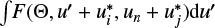$\int F\left(\text{Θ},u^{\prime }+u_i^{\ast },u_n+u_j^{\ast }\right)\text{d}{u}^{\prime }$ for all couples (i, j). This means that the selection of ${\left\{u_{n^{\prime }}\right\}}_{n^{\prime }=1}^{N_{v^{\prime }}}$ only depends on r, Θ, u, and $u_i^{\ast }$ ¹⁰. This property of the spectral quadrature allows us to reduce the number of interpolations of I required to evaluate the emissivity.

The strategy adopted in this work, which is detailed in Appendix C, can be summarised as follows: if Θ = 0, then $F\left(0,u,u^{\prime }\right)=\sqrt{\pi }\delta \left(u-u^{\prime }\right)W\left(a,u^{\prime }\right)$ and the integral $$\int F\left(\text{Θ},u^{\prime }+u_{k_u,k_{\mathcal{l}}},u_n+u_{k_u,k_{\mathcal{l}}^{\prime }}\right)\mathit{I}\left(r,{\Omega }^{\prime },u^{\prime }-u_{\text{b}}\left({\Omega }^{\prime }\right)\right)\text{d}{u}^{\prime }$$(11) is carried out analytically. Otherwise, if Θ is small or − u_n is far from all $u_i^{\ast }$, we used a Gauss-Hermite quadrature with 65 nodes, thus exploiting property (d). In all other cases, we are either in the line-core (e) or in the near-wing (f) regimes, and we adopted a GL quadrature with a number of nodes that depends on Θ and $\left|u_n+u_i^{\ast }\right|$. An additional strategy adopted in this work to further diminish the number of evaluations of the Faddeeva function is presented in Appendix D.

As illustrative examples, the left panel of Fig. 1 shows the frequency quadrature nodes as dots for the case of a single cluster with u^∗ = −11.15. The central panel displays the number of frequency nodes $N_{v^{\prime }}$ generated with $u_1^{\ast }=-11.15$ and $u_2^{\ast }=20$ for different u_n and Θ. Finally, the right panel illustrates the relative error of evaluating Eq. (11) with the strategy outlined above, with I = (1, 0, 0, 0), a = 0.01, $u_{k_u,k_{\mathcal{l}}}=u_{k_u,k_f^{\prime }}=-11.1,u_1^{\prime }=-11.15$, and $u_2^{\ast }=20$ ¹¹. Notably, with about 100−300 spectral quadrature nodes, we obtain a relative error that is always smaller than 10⁻⁸.

Concerning the ${\overline{\mathcal{R}}}^{\text{III }}$ redistribution function, the situation is much simpler than for its ${\overline{\mathcal{R}}}^{\text{II}}$ counterpart, as the incident and emergent frequencies are totally uncorrelated (see Sect. 2.4). Therefore, for the numerical integration of ${\overline{\mathcal{R}}}^{\text{III }}$ I over frequency, it is possible to choose a quadrature grid independent of r, Θ, and u_n. In the following, we consider a single GL rule with 2001 nodes in the interval [ − 200, 200].

We note that when evaluated numerically, Eq. (2) should be suitably normalised to avoid spurious sources or sinks of photons (e.g. Adams et al. 1971). In Appendix E, we show how the generalised Kirchhoff’s law can be used to perform this task. This method is presently used to normalise the intensity component of the emission vector when computing the results presented in Sect. 6. By applying this procedure, we improved both the accuracy of the results and the robustness of the iterative method.

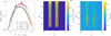Fig. 1 Illustrative examples of the quadrature grids. Left: real part (blue and red lines) and positive and negative values of the imaginary part (yellow and purple lines, respectively) of F as a function of $u^{\prime }-\left(u_n+u_{k_{\ell },k_{\ell }^{\prime }}\right)$, with u′ = u(ν′), un = u(νn), and $u_{k_{\ell },k_{\ell }^{\prime }}=u_{k_u,k_{\ell }^{\prime }}-u_{k_u,k_{\ell }}$, for different values of $u+u_{k_u,k_{\ell }^{\prime }}$. Here, a = 0.01, Θ = 0.9π, $u_{k_u,k_{\ell }}=-11.1$, and $u_{k_u,k_f^{\prime }}=-11.2$. The dots denote the quadrature nodes un′ generated with u∗ = −11.15. Centre: number of quadrature nodes as a function of un and Θ, with a = 0.01, $u_1^{\ast }=-11.15$, and $u_2^{\ast }=20$. Right: logarithm of the relative error of evaluating Eq. (11) with the quadrature nodes of the central panel with respect to the reference values obtained with the Gauss–Kronrod adaptive method, with I = (1, 0, 0, 0), a = 0.01, and $u_{k_u,k_{\ell }}=u_{k_u,k_{\ell }^{\prime }}=-11.1$.

5 Iterative solution strategy

The considered RT problem has been recast in the linear system given by Eq. (8), for which we have to find a solution. Given the size of the system (N ∼ 10⁷ for small-scale 1D applications, see Sect. 6.2) and that the matrix Id − ΛΣ in Eq. (8) is dense, the use of direct matrix inversion methods is unfeasible. Thus, the application of an iterative solution strategy is necessary.

5.1 Matrix-free iterative methods

Krylov methods are well suited for matrix-free approaches and proved to be highly effective solution strategies in the RT context for large linear systems (e.g. Jolivet et al. 2021; Benedusi et al. 2021, 2023). In the present work, we thus considered the generalised minimal residual (GMRES) iterative method in its matrix-free version. For increased flexibility, we also explored other iterative solution strategies, such as the Richardson and the alternating Anderson-Richardson (AAR) methods (Hackbusch 1994; Suryanarayana et al. 2019). We monitored the convergence of the iterative methods by evaluating the relative residual $$\text{res }=\frac{||\mathit{\text{Λ}}{\mathit{\epsilon }}^{th}+\mathit{t}-(Id-\text{ΛΣ}){\mathit{I}}_{||}}{||\text{Λ}{\mathit{\epsilon }}^{th}+{\mathit{t}}_{||}},$$ taking as a stopping criterion res < tol for a given tolerance, tol.

5.2 Preconditioning

Preconditioning of linear systems can significantly increase robustness and convergence speed of iterative techniques. Given P ∈ ℝ ^N×N a non-singular matrix, the left preconditioning¹² of Eq. (8) was obtained by considering the equivalent system $$P^{-1}(Id-\text{ΛΣ})\mathit{I}=P^{-1}\left(\text{Λ}{\mathit{\epsilon }}^{th}+t\right).$$

We emphasise that to be effective, P should be a good and computationally cheap approximation of the operator Id − ΛΣ. Janett et al. (2024) showed that when dealing with RT problems for polarised radiation including AD PRD effects, common algebraic preconditioners, such as Jacobi and SOR, are out-performed by tailored physics-based preconditioners, that is, operators corresponding to a simplified physical setting of the considered problem. Crucially, physics-based preconditioners do not require the explicit algebraic description of the operators of interest and are very intuitive to implement. In our RT problem, we can write physics-based preconditioners as $$P=\mathit{I}d-{\text{Λ}}^{\ast }{\text{Σ}}^{\ast },$$ where Λ^∗ and Σ^∗ encode the approximations of Λ and Σ.

A variety of simplifications can be adopted to design Σ^∗. For instance, a common approach to lower the computational complexity of Σ is to consider the so-called AA approximation (e.g. Mihalas 1978; Rees & Saliba 1982; Bommier 1997b). Within this approximation, the redistribution function in the co-moving frame describing scattering processes that are coherent in frequency in the atomic rest frame can be written as $${\overline{\mathcal{R}}}_Q^{II-AA,K{K}^{\prime }}\left(v^{\prime },v\right)=\frac{1}{2}{\int }_0^{\pi }\sin (\text{Θ}){\overline{\mathcal{R}}}_Q^{II,K{K}^{\prime }}\left(\text{Θ},v^{\prime },v\right)\text{dΘ}.$$(12)

Remarkably, this redistribution function is independent of propagation directions and only couples the frequencies of the incident and scattered radiation. We note that the AA approximation is not only useful in the context of physics-based preconditioners, but it also yields reliable results when applied to the modelling of the intensity spectra of strong resonance lines (see Leenaarts et al. 2012; Sukhorukov & Leenaarts 2017). As far as scattering polarisation is concerned, the AA approximation can either provide satisfactory results (e.g. Riva et al. 2024; del Pino Alemán et al. 2024), or introduce large and hardly predictable inaccuracies (e.g. Sampoorna et al. 2017; Janett et al. 2021a; Belluzzi et al. 2024). For this reason, it is always important to carefully assess its suitability under different conditions, as discussed in Sect. 6.6 for the H I Ly-α line.

To further simplify Λ^∗ and Σ^∗, it is also possible to neglect polarisation and magnetic fields, or assume an isotropic emission vector in the co-moving frame (Benedusi et al. 2022; Janett et al. 2024). Finally, we note that the application of P⁻¹ itself requires solving a linear system of the form Px = y. This is presently achieved iteratively with a matrix-free iterative method, meaning that the whole linear problem is solved by means of two nested iterative solvers. To further enhance the performance of our solution strategy, we also implemented the possibility of preconditioning the linear system Px = y, as detailed in Appendix F.

6 Numerical applications

The solution strategy outlined in Sects. 2–5 was implemented in TRAP⁴ as a MATLAB (MATLAB 2023) routine, considering plane-parallel 1D models, and parallelised by spatially decomposing the calculation of ε^sc across threads. Hereafter, we discuss concrete applications of TRAP⁴. Specifically, after presenting the atmospheric and atomic models and the numerical setting, we investigate the numerical error affecting our results, we perform a benchmark with the HanleRT-TIC¹³ code (del Pino Alemán et al. 2016, 2020), and we discuss the suitability of using the PRD–AA approximation with respect to full AD calculations. For our applications, we considered the following chromospheric resonance lines whose modelling requires the inclusion of both PRD effects and J-state interference: the Mg II h&k doublet at 2800 Å and the H I Ly-α line at 1216 Å. For sake of conciseness, in the following we do not discuss Stokes V, although it is always included in our calculations.

6.1 Atmospheric and atomic models

In this work, calculations were carried out in a 1D plane-parallel domain extracted from the semi-empirical atmospheric model C (hereafter FAL-C) of Fontenla et al. (1993), which fully contains the formation region of the considered spectral lines. Even if 1D, this model is sophisticated enough to test our strategy and assess the suitability of using the AA approximation to model wavelength-integrated scattering polarisation signals of the H I Ly-α line.

In the following, we consider the contribution to the Doppler width due to non-thermal microturbulent velocity: $$\text{Δ}{v}_{\text{D}}(z)=\frac{v_0}{c}\sqrt{\frac{2k_{\text{B}}T(z)}{M}+\xi {(z)}^2},$$ where T is the temperature, M the mass of the atom, and ξ the microturbulent velocity determined according to Fontenla et al. (1991). Moreover, for the sake of generality, some calculations were carried out in the presence of magnetic and bulk velocity fields, which were added ad-hoc to the atmospheric model, as detailed in the following subsections.

The Mg II h&k lines result from two distinct fine-structure transitions between the ground level of ionised magnesium 3s²S_1/2 and the first excited term composed by the levels $3{\text{p}}^2{\text{P}}_{1/2}^{\text{o}}$ and $3{\text{p}}^2{\text{P}}_{3/2}^o$. These two fine-structure components are separated by 7 Å and give thus rise to two well distinct lines. The H I Ly-α line also results from two distinct fine-structure transitions, between the ground level of hydrogen 1s ²S_1/2 and the excited term composed by the levels $2{\text{p}}^2{\text{P}}_{1/2}^o$ and $2{\text{p}}^2{\text{P}}_{3/2}^o$ ¹⁴. Contrary to the Mg II h&k lines, these two fine-structure components are separated by 6 mÅ only, and are thus completely blended. The relevant atomic parameters for the Mg II h&k doublet and the H I1 Ly-α line are provided in Table 1.

In addition to the atmospheric and atomic parameters, TRAP⁴ also requires as input quantities the broadening constants Γ_R, Γ_I, Γ_E, and the lower-level or term population of the considered transition. For all our calculations, we used Γ_R = A_uℓ, with A_uℓ the Einstein coefficient for spontaneous emission from the upper to the lower term (see Table 1). For Mg II, we calculated the ground-level population using the HanleRT-TIC code, neglecting polarisation and considering a static unmagnetised atmosphere and a two-term atom with AD PRD effects. The same code was also used to calculate the Γ_E and Γ_I broadenings, as well as the continuum coefficients κ^c, σ^c, and ε^c,th (see Appendix A). In particular, Γ_E accounts for elastic collisions with both neutral hydrogen and helium perturbers via Van der Waals interactions and the quadratic Stark effect, while Γ_I is calculated treating inelastic collisions in a two-term atom following Belluzzi et al. (2013). For H I Ly-α, we used the hydrogen ground-level population tabulated in the FAL-C model. The broadening due to inelastic de-exciting collisions was evaluated as Γ_I = N_eQ_ul, with N_e the electron density from the FAL-C model and $$Q_{ul}(z)=8.63\cdot {10}^{-6}\frac{v(z)}{g_u\sqrt{T(z)}},$$ where g_u = 8 is the degeneracy of the upper level with principal quantum number n = 2 and the coefficient v (which depends on T ) is taken according to Przybilla & Butler (2004). Furthermore, Γ_E was computed with the RH code (Uitenbroek 2001), fixing the hydrogen ground-level population to the value provided by the FAL-C model and considering collisions with neutral hydrogen and helium perturbers via both linear and quadratic Stark effects. The values of κ^c, σ^c, and ε^c,th were also computed with RH. A similar procedure was used to initialise the H I Ly-α calculations in Alsina Ballester et al. (2022).

6.2 Physical and numerical parameters

Concerning the spectral grid, we used 210 wavelength nodes in the interval [2705.5 Å, 2901.2 Å] for the Mg II h&k doublet and 191 wavelength nodes in the interval [1184.5 Å, 1248.6 Å] for the H I Ly-α line. For the angular discretisation, we used nine nodes uniformly distributed in χ, whereas we used two sets (one for each hemisphere) of six GL nodes for the heliocentric angles µ = cos(θ), for a total N_Ω = 108. Given that N_r = 70 for the FAL-C atmospheric model, the RT problem in Eq. (8) thus had N = 4N_rN_νN_Ω ∼ 6 · 10⁶ degrees of freedom for both atomic models. We note that the chosen grids correspond to a number of scattering angles $N_{\text{Θ}}=205\ll N_{\text{Ω}}^2=11664$ and an averaged number of spectral quadrature nodes $N_{v^{\prime }}\simeq 133$ and $N_{v^{\prime }}\simeq 127$ for Mg II and H I, respectively. Presently, all inter-polations between the observer’s and the co-moving frame (and vice versa) are performed in terms of cubic splines.

Concerning the formal solver, we used the BESSER exponential integrator for the Mg II h&k doublet, consistently with the recent work by del Pino Alemán et al. (2024). On the other hand, we used the DELOPAR exponential integrator for the H I Ly-α line, to allow direct comparisons with previous works in the literature (e.g. Alsina Ballester et al. 2022). As the BESSER integrator introduces some small non-linearity into the problem due to the source vector interpolation used to avoid overshooting (see the definition of the control points in Štěpán & Trujillo Bueno 2013), we opted for the AAR iterative method with tol = 10⁻⁹ for the Mg II h&k doublet, whereas we used GMRES with tol = 10⁻¹⁰ for the H I Ly-α line. After reaching the desired tolerance, we performed an additional formal solution to compute the final results at specific directions that are not part of the angular grid.

With the above numerical parameters, the code employed approximately 1700 s for the Mg II h&k doublet and 1450 s for the H I Ly-α line to perform a single preconditioned iteration on an Intel Xeon CPU E5-1620. Overall, for both atomic mod-els, the largest fraction of the computational time was spent for evaluating ε^ℓ,sc, which took about 1300 s per iteration. Thanks to our solution strategy, only 25% of this time was spent in evaluating the Faddeeva function, whereas approximately 55 − 60% of it was employed to interpolate I to the spectral quadrature grid and assemble $W_{k_u,k_{\mathcal{l}}}$ in Eq. (D.1). Moreover, by employing the block-diagonal preconditioner introduced in Appendix F, we ensured that less than 20% of the full solution time was spent in pre-conditioning the system. Finally, given the high performances of physics-based preconditioned methods, the target tolerance was reached with only 10–12 iterations when starting from a zero initial guess.

6.3 Solution verification

Before using any numerical results to perform a physical investigation, it is essential to assess if they are accurate enough for their intended use. This task is known as solution verification. In this respect, we note that the tolerances specified in Sect. 6.2 are very conservative, thus ensuring unnoticeable differences in the emerging profiles when further reducing tol by an order of magnitude. Moreover, besides carrying out the reference calculations with numerical parameters as given in Sect. 6.2, we carried out three additional calculations for both the Mg II h&k doublet and the H I Ly-α line: one with doubled spatial resolution, where we introduced a new set of grid points equidistant to each pair of adjacent original points and interpolated the input variables to the new grid; one with increased angular resolution, with fifteen azimuths and two sets of ten GL inclinations for a total N_Ω = 300; and one with doubled N_ν. For all these calculations, we considered a static atmosphere with a height-independent horizontal (χ_B = 0 and θ_B = π/2) magnetic field of 20 and 50 G for the Mg II h&k doublet and the H I Ly-α line, respectively.

The resulting profiles for a LOS µ = 0.1 are shown in Fig. 2. In general, we see an excellent agreement between the black solid (reference calculations) and the colour lines¹⁵. Minor discrepancies are observed away from the line cores, in particular in the fractional linear polarisation signals of the H I Ly-α line. These extremely small discrepancies suggest that the reference calculations are at convergence in resolution. Moreover, the profiles look very similar to other computations in the literature (compare to Figs. 3 and B.3 of Alsina Ballester et al. 2022, for the Mg II h&k doublet and the H I Ly-α line, respectively), thus increasing the reliability of our results. We also carried out an additional set of computations (not shown in Fig. 2 for clarity), where we used the highly accurate (though more time-consuming) adaptive Gauss–Kronrod method for integrating Eq. (D.1) over frequency. Negligible differences with respect to the reference emergent profiles were found.

Fig. 2 Intensity (left column), Q/I (middle column), and U/I (right column) as a function of vacuum wavelength for the Mg II h&k doublet (first row) and the H I Ly-α line (second row), obtained with PRD–AD calculations in a static magnetic FAL-C atmosphere (see text) for a LOS with µ = 0.1. The solid black curves correspond to reference calculations, whereas the red (dashed), yellow (dot-dashed), and purple (dotted) lines are the results of calculations with increased spatial, angular, and frequency resolution, respectively. The reference direction for positive Stokes Q is the parallel to the limb.

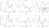Fig. 3 Intensity (left column), Q/I (middle column), and U/I (right column) as a function of vacuum wavelength for the Mg II k line obtained with PRD–AA (dashed lines) and PRD–AD (solid lines) calculations in a dynamic magnetic atmosphere (see text) for the two LOSs with µ = 0.1 (first row) and µ = 1 (second row). The blue and red curves correspond to calculations carried out with the HanleRT-TIC and the TRAP4 code, respectively. The reference direction for positive Stokes Q is the parallel to the limb.

6.4 Benchmark with the HanleRT-TIC code

To verify the TRAP⁴ code, we performed a benchmark study for the Mg II h&k doublet with the HanleRT-TIC code. We recall that the two codes are based on different theoretical frameworks, so that the form of the redistribution matrices R^II and R^III is not exactly the same. Moreover, they use different frequency grids, quadrature grids, and iterative solution methods. Also the way of normalising the emissivity is different.

For this test, we considered a height-independent horizontal (χ_B = 0 and θ_B = π/2) magnetic field of 20 G. Moreover, to increase the complexity of the problem, we added a bulk velocity to the atmospheric model, with the vertical component mimicking Fig. 1 of del Pino Alemán et al. (2024) and defined as $$v_z=-10\cdot e^{-{[(z-2100)/500]}^2}\cdot \left[1+\text{erf}\left(\frac{2100-z}{150}\right)\right]\text{, }$$ the horizontal components given by $$v_x=0.7\left|v_z\right|\cos \left({\chi }_v\right)\hspace{1em}\text{ and }\hspace{1em}{v}_y=0.7\left|v_z\right|\sin \left({\chi }_v\right)\text{, }$$ and $${\chi }_v=-2\pi \frac{z-z_{\min }}{z_{\max }-z_{\min }}+\pi ,$$ where z_min = − 100 km and z_max = 2219.43 km and z is given in kilometres. We then solved the RT problem with the TRAP⁴ and HanleRT-TIC codes for the AA and AD cases.

The results are shown in Fig. 3 for the k line at the two LOSs µ = 0.1 (first row) and µ = 1 (second row), with the latter denoting a forward-scattering geometry (see, e.g. Belluzzi et al. 2024). Here, we only focus on the k line, as it is the spectral region showing the largest discrepancies between the results of the two codes. Overall, we found very satisfying agreement between HanleRT-TIC (blue curves) and TRAP⁴ (red curves), in particular for the fractional polarisation signals (middle and right columns). On the other hand, relative differences of the order of 5 − 10% are visible in I near the k line core. This discrepancy is probably related to the different normalisation of the emissivity and formulation of the redistribution matrices used in the two codes.

The comparison between the PRD–AA (dashed lines) and PRD–AD (solid lines) results reveals once more the importance of using an AD description of scattering processes when modelling the Mg II h&k doublet in a dynamic and magnetic atmosphere, as discussed in great detail in del Pino Alemán et al. (2024). Indeed, it is particularly important in order to accurately model the forward-scattering Hanle effect (see Q/I and U/I at µ = 1, as well as the discussion in Belluzzi et al. 2024).

6.5 Validation of the two-step approach

It is important to note that in agreement with our assumption that polarisation has a negligible impact on the ground-level population of Mg II, the input parameters of the TRAP⁴ code were obtained from HanleRT-TIC PRD calculations for a static, unmagnetic atmosphere and neglecting polarisation, as detailed in Sect. 6.1. On the other hand, the HanleRT-TIC results in Fig. 3 (blue lines) were obtained calculating the ground-level population in a self-consistent way, accounting for the impact of polarisation, magnetic fields, and velocities. Remarkably, we found relative differences in the ground-level populations between the two cases that are below 0.2%. A detailed investigation also revealed that these extremely small differences do not play any role in the Stokes profiles computed with TRAP⁴. This fact, in combination with the excellent agreement between the HanleRT-TIC and TRAP⁴ results of Sect. 6.4, is thus a validation of the working assumptions discussed in Sect. 2.5 and of our solution strategy.

6.6 Impact of PRD–AD on the Ly-α line

As an application of broad physical interest, we also investigated the suitability of using the AA approximation when modelling wavelength-integrated scattering polarisation signals of the H I Ly-α line, as done by Alsina Ballester et al. (2023). To this aim, we computed the emergent Stokes profiles of the H I Ly-α line obtained with a static magnetic atmosphere, with height-independent horizontal magnetic fields of different strengths B = 0, 10, 25, 50, and 100 G, both within the PRD–AA and PRD–AD descriptions. Then, following Alsina Ballester et al. (2023), synthetic narrow-band signals are obtained by weighting by a Gaussian the numerical emergent Stokes profiles and integrating the results over wavelength. Namely, $$\overline{X}(\mu )=\frac{1}{\sqrt{2\pi }{\sigma }_{\lambda }}{\int }_{{\lambda }_0-\text{Δ}\lambda }^{{\lambda }_0+\text{Δ}\lambda }\exp \left(-\frac{{\left(\lambda -{\lambda }_0\right)}^2}{2{\sigma }_{\lambda }^2}\right)X\left(z_{\max },\mu ,\lambda \right)\text{d}\lambda ,$$ where X = I, Q, and U; λ₀ = 1215.67 Å is the H I Ly-α line-centre wavelength in vacuum; and σ_λ is the standard deviation of the Gaussian weighting function, selected so that it corresponds to a full width at half maximum of $2\sqrt{2\log (2)}{\sigma }_{\lambda }=35Å$. For the present study, we considered as integration limit Δλ = 30 Å (see Alsina Ballester et al. 2023, for a discussion of the impact of Δλ on the results).

The resulting centre-to-limb profiles are displayed in Fig. 4, with dashed and solid lines for PRD–AA and PRD–AD calculations, respectively. Overall, there is excellent agreement between PRD–AA and PRD–AD results. Minor discrepancies are found, in particular for Ū/Ī near disk centre (µ ∼ 1), but their amplitude is small. We also repeated the computations for different values of Δλ and with the atmospheric models A, F, and P of Fontenla et al. (1993), finding negligible differences between PRD–AA and PRD–AD results.

Fig. 4 Centre-to-limb variation of $\overline{Q}/\overline{I}$ (left panel) and Ū/Ī (right panel) as a function of µ = cos(θ). The results are obtained for χ = 0 and considering height-independent horizontal (θB = π/2 and χB = 0) magnetic fields of different strengths (see the legend). Dashed and solid lines correspond to PRD–AA and PRD–AD calculations, respectively.

7 Conclusions

In the present paper, we have illustrated an accurate and effective solution strategy to model the Stokes profiles of strong resonance lines originating in the solar atmosphere while taking into account scattering polarisation with PRD effects in their general AD formulation, J-state interference, and the impact of arbitrary magnetic fields and bulk velocities. The formalism we have introduced can be applied to the two-level and two-term atoms, and it can also be used for the inclusion of the atomic hyperfine structure. Moreover, although we applied the formalism to 1D plane-parallel atmospheric models, it can be easily generalised to 3D geometries (see Benedusi et al. 2023).

After introducing the new formalism, we introduced a suitable physical approximation, thanks to which the problem became linear in the radiation field I. The approximation consists of assuming that polarisation has a negligible impact on the population of the lower level or term of resonance lines so that it can be retrieved from independent unpolarised calculations and considered as an input parameter of the problem. Together with a suitable algebraic formulation of the problem, this allowed us to exploit the innovative physics-based preconditioners of Janett et al. (2024) and efficiently solve the problem with matrix-free preconditioned algorithms. Since the computational time necessary to apply the physics-based preconditioner to the full problem can be a large fraction of the full time to solution, we also introduced an additional block-diagonal preconditioner, which we successfully used to speed up the calculations.

To accelerate the calculations in the presence of bulk velocities, we computed the scattering emissivity in the co-moving frame and then interpolated it to the observer’s frame. This strategy drastically reduces the required number of evaluations of the redistribution functions. Moreover, we presented a careful choice of the angular and spectral quadrature nodes that, in combination with a proper normalisation of the scattering emissivity, allowed for a solution of the problem that is at the same time fast and accurate.

We applied the presented solution strategy to the synthesis of the Stokes profiles of the Mg II h&k doublet and the H I Ly-α line. In particular, considering the 1D FAL-C atmo-spheric model, we performed a solution verification of the emerging synthetic profiles, showing that for the considered numerical parameters, the results are solid and the numerical errors considerably small. A detailed benchmark of TRAP⁴ with HanleRT-TIC results also displayed good agreement between the two codes. This is a remarkable validation of the linearisation strategy outlined in Sect. 2.5.

Finally, wavelength-integrated polarisation profiles of the H I Ly-α line show excellent agreement when comparing PRD– AA and PRD–AD calculations. The very minor discrepancies between the two computations suggest that a complete PRD– AD description of scattering processes is not strictly necessary to accurately model the impact of magnetic fields with B ≤ 100 G on these signals, thus validating the work of Alsina Ballester et al. (2023). However, this comparison was limited to 1D plane-parallel atmospheric models, and it will be important to verify whether this conclusion also remains valid in comprehensive 3D models, for example by implementing the presented solution strategy in the novel 3D numerical framework of Benedusi et al. (2023).

Acknowledgements

The financial support by the Swiss National Science Foundation (SNSF) through grant CRSII5_180238 is gratefully acknowledged. T.P.A., E.A.B., and J.T.B. acknowledge support from the Agencia Estatal de Investigación del Ministerio de Ciencia, Innovación y Universidades (MCIU/AEI) under grant “Polarimetric Inference of Magnetic Fields” and the European Regional Development Fund (ERDF) with reference PID2022-136563NB-I00/10.13039/501100011033. E.A.B. acknowledges support from the European Research Council through the Synergy grant No. 810218 (“The Whole Sun” ERC-2018-SyG). T.P.A.’s participation in the publication is part of the Project RYC2021-034006-I, funded by MICIN/AEI/10.13039/501100011033, and the

European Union “NextGenerationEU”/RTRP. We also sincerely thank the referee for the careful reading of the manuscript and the many comments, which greatly helped us to improve the quality of the paper.

Appendix A Continuum processes

Under typical conditions of the solar atmosphere, it is a good approximation to assume that continuum processes do not contribute to dispersion and dichroism, that is, to the off-diagonal elements of K (e.g. Landi Degl’Innocenti & Landolfi 2004). Additionally, the continuum contribution to the diagonal elements of K (continuum opacity) is given by ${\eta }_1^c(r,v)={\kappa }^c(r,v)+{\sigma }^c(r,v)$, where κ^c and σ^c are the isotropic extinction coefficients for true absorption and scattering, respectively, and the superscript c denotes continuum contributions.

Concerning the continuum emissivity, we consider both thermal and scattering processes, for which we make the assumption of coherent scattering in the observer’s frame. This implies that the continuum contribution to the emissivity can be written as $$\begin{array}{c}{\mathit{\epsilon }}^c(\mathit{r},\Omega ,v)={\mathit{\epsilon }}^{c,\text{ th }}(\mathit{r},v)+{\sigma }^c(\mathit{r},v)\sum _{K,Q}{(-1)}^Q{\mathcal{T}}_Q^K(\Omega )\\ \times \oint {\mathcal{T}}_{-Q}^K\left({\Omega }^{\prime }\right)\cdot I\left(\mathit{r},{\Omega }^{\prime },v\right)\frac{\text{d}{\Omega }^{\prime }}{4\pi },\end{array}$$ where ε^c,th is the continuum thermal emissivity (which is isotropic and only contributes to Stokes I) and 𝒯 is a vector whose four components are the polarisation tensors (see Section 5.11 of Landi Degl’Innocenti & Landolfi 2004) in the four Stokes parameters. We note that κ^c, σ^c, and ε^c,th are currently evaluated with publicly available routines (e.g. Uitenbroek 2001; Li et al. 2022).

Appendix B

$A_Q^{K{K}^{\prime }},B_Q^{K{K}^{\prime }}$, and branching ratios

The quantity $A_Q^{K{K}^{\prime }}$ appearing in Eq. (3) is defined as $$A_Q^{K{K}^{\prime }}\left(\mathit{r},k_u,k_u^{\prime },k_{\mathcal{l}},k_{\mathcal{l}}^{\prime }\right)=\frac{{\alpha }_{k_u,k_u^{\prime }}(\mathit{r})}{2\pi \text{Δ}{v}_D{(\mathit{r})}^2}{\mathcal{A}}_Q^{K{K}^{\prime }}\left(k_u,k_u^{\prime },k_{\mathcal{l}},k_{\mathcal{l}}^{\prime }\right),$$ where ${\alpha }_{k_u,k_u^{\prime }}$ represents the branching ratio for scattering processes described by ℛ ^II (it contains both the branching ratio between thermal and scattering processes and the one between ℛ ^II and ℛ ^III) and ${\mathcal{A}}_Q^{K{K}^{\prime }}$ is a quantity depending on a series of quantum numbers characterising the involved atomic states.

According to the works of Bommier (1997a,b, 2017), the branching ratio for ℛ ^II is given by $${\alpha }_{k_u,k_u^{\prime }}(\mathit{r})=\frac{{\Gamma }_{\text{R}}}{{\Gamma }_{\text{R}}+{\Gamma }_{\text{I}}(\mathit{r})+{\Gamma }_{\text{E}}(\mathit{r})+2\pi i{v}_{k_u,k_u^{\prime }}(\mathit{r})}.$$

With this definition and taking ${\mathcal{A}}_Q^{K{K}^{\prime }}\left(k_u,k_u^{\prime },k_{\mathcal{l}},k_{\mathcal{l}}^{\prime }\right)=C_{QK{K}^{\prime }{M}_u{M}_u^{\prime }{M}_{\mathcal{l}}{M}_{\mathcal{l}}^{\prime }p{p}^{\prime }{p}^{″}{p}^{‴}}$ (see Eq. (12) of Bommier 1997b), one recovers an expression for ${\mathcal{R}}_Q^{II,K{K}^{\prime }}$ fully analogous to Eq. (23) of Alsina Ballester et al. (2017) for the two-level atom. Similarly, by considering ${\mathcal{A}}_Q^{K{K}^{\prime }}\left(k_u,k_u^{\prime },k_{\mathcal{l}},k_{\mathcal{l}}^{\prime }\right)={\mathcal{A}}_Q^{K{K}^{\prime }}\left(j_u{M}_u,j_u^{\prime }{M}_u^{\prime },j_{\mathcal{l}}{M}_{\mathcal{l}},j_{\mathcal{l}}^{\prime }{M}_{\mathcal{l}}^{\prime }\right)$ (see Eq. (C.19) of Alsina Ballester et al. 2022), one recovers the redistribution functions in Eq. (10) of Alsina Ballester et al. (2022) for a two-term atom.¹⁶

The quantity $B_Q^{K{K}^{\prime }}$ appearing in the definition of ${\mathcal{R}}_Q^{III,K{K}^{\prime }}$, Eq. (5), is defined as $$B_Q^{K{K}^{\prime }}\left(\mathit{r},k_u,k_u^{\prime },k_{\mathcal{l}},k_{\mathcal{l}}^{\prime }\right)=\frac{{\beta }_{k_u,k_u^{\prime }}(\mathit{r})-{\alpha }_{k_u,k_u^{\prime }}(\mathit{r})}{4\pi \text{Δ}{v}_D{(\mathit{r})}^2}{\mathcal{A}}_Q^{K{K}^{\prime }}\left(k_u,k_u^{\prime },k_{\mathcal{l}},k_{\mathcal{l}}^{\prime }\right),$$ where the term ${\beta }_{k_u,k_u^{\prime }}-{\alpha }_{k_u,k_u^{\prime }}$ is the branching ratio for ℛ^III, with $${\beta }_{k_u,k_u^{\prime }}(\mathit{r})=\frac{{\Gamma }_{\text{R}}}{{\Gamma }_{\text{R}}+{\Gamma }_{\text{I}}(\mathit{r})+2\pi i{v}_{k_u,k_u^{\prime }}(\mathit{r})}.$$

Here, we assumed that the depolarising effect of elastic collisions is negligible. Notably, this is a good approximation when modelling the polarisation of strong resonance lines that form in the low-density plasma of the solar chromosphere (Alsina Ballester et al. 2021). We note that the expression we provided for ${\beta }_{k_u},k_u^{\prime }$ holds both for a two-level atom (Bommier 1997b) and for a two-term atom (Bommier 2017) and include the term 1 − ϵ.

If depolarising collisions are not negligible, the redistribution matrix formalism cannot be used for a two-term atomic model, as the SE equations do not have a closed analytic solution (unless magnetic fields and collisional transitions between different J-levels of the same term are neglected; see Bommier 2017). However, the redistribution matrix can be derived also accounting for depolarising collisions in the case of a two-level atom (see Bommier 1997b), the only difference being in the ${\beta }_{k_u,k_u^{\prime }}$ factor, which takes the form $${\beta }_{k_u,k_u^{\prime }}^{(K)}(\mathit{r})=\frac{{\Gamma }_{\text{R}}}{{\Gamma }_{\text{R}}+{\Gamma }_{\text{I}}(\mathit{r})+D^{(K)}(\mathit{r})+2\pi i{v}_{k_u,k_u^{\prime }}(\mathit{r})},$$ with D^(K) the depolarisation rate due to elastic collisions. With these branching ratios, one recovers the expressions for ℛ ^III in Eq. (20) of Alsina Ballester et al. (2017) and in Eq. (11) of Alsina Ballester et al. (2022) for two-level and two-term atoms, respectively.

Appendix C Spectral quadrature grid for ℛ^II

Here, we detail the spectral quadrature grids ${\left\{u_{n^{\prime }}\right\}}_{n^{\prime }=1}^{N_{y^{\prime }}}$ used to numerically evaluate Eq. (11). Recalling that u_n denotes a discrete point of the reduced frequency grid, these are defined as follows:

1. if Θ = 0, Eq. (11) is integrated analytically;

2. if Θ ≥ π/8 or min $\left|u_n+u_i^{\ast }\right|\ge u^{\text{t}}$, case (d) in Sect. 4.3, we use a Gauss-Hermite quadrature with 65 nodes;

3. if Θ > π/8 and $\left|u_n+u_i^{\ast }\right|\le 2$, we are in the line-core regime, case (e) in Sect. 4.3, and we distinguish between the three different cases

   • π/8 ≤ Θ ≤ π/2, for which a single GL quadrature of 101 nodes over the interval [u^M − Δ¹, u^M + Δ¹] is used,

   • π/2 < Θ ≤ 15π/16, for which three contiguous GL quadratures of 55, 81, and 55 nodes over the intervals [u − Δ¹, u^M− Δ²], [u^M − Δ², u^M + Δ²], and [u^M + Δ², u + Δ¹], respectively, are used, and

   • 15π/16 < Θ < π, for which four contiguous GL quadratures of 65, 101, 101, and 65 nodes over the intervals [u − Δ¹, u^M− Δ³], [u^M − Δ³, u^M], [u^M, u^M + Δ³], and [u^M + Δ³, u + Δ¹], respectively, are used;

4. if Θ > π/8 and $2<\underset{i}{\min }\left|u_n+u_i^{\ast }\right|<u^{\text{t}}$, we are in the nearwing regime, case (f) in Sect. 4.3, and we combine three GL contiguous quadratures of 55, 95, 121 nodes (121, 95, 55 if $u_n+u_i^{*}<0$ over the intervals [L^nw, u^M − Δ⁴], [u^M − Δ⁴, u^M + Δ⁴], and [u^M + Δ⁴, R^nw], respectively.

Here, we introduced the threshold u^t = max(5.8, 2.5 Θ) and we defined $u^{\text{M}}=\left(u_n+u_i^{*}\right)\cos (\Theta )-u_i^{*}$, Δ¹ = 11 sin(Θ/2), Δ² = 6(0.1 + a + cos(Θ/2))/(a + 1), Δ³ = 6(0.05 + a + cos(Θ/2))/(a + 1), Δ⁴ = 6 cos(Θ/2) + 0.2, L^nw = min(u^M − Δ⁴ 1, ũ − Δ¹), and R^nw = max(u^M + Δ⁴ + 1, ũ + Δ¹), where $u_i^{*}$ is the cluster centre closest to − u_n, and ũ = u_Re and ũ = u_Im for the real and imaginary parts of Eq. (11), respectively, are $$\begin{array}{c}{u}_{\mathrm{Re}}=sign\left(u_n+u_i^{\ast }\right)\sqrt{{\left(u_n+u_i^{\ast }\right)}^2-4{\sin }^2(\text{Θ}/2)},\\ u_{Im}=sign\left(u_n+u_i^{\ast }\right)\sqrt{{\left(u_n+u_i^{\ast }\right)}^2-2{\sin }^2(\text{Θ}/2)}.\end{array}$$

Concerning the AA approximation, the integral over Θ in Eq. (12) smooths out the sharp peaks and sign reversals of ${\overline{\mathcal{R}}}^{II}$ near Θ = 0 and Θ = π, thus simplifying the numerical integration of ${\overline{\mathcal{R}}}^{II-AA}\cdot I$ over frequency with respect to the general AD case. The integral in Eq. (12) also drastically reduces the degree of freedom of the redistribution function, removing its dependence on Θ and making it possible to assemble ${\overline{\mathcal{R}}}^{II-AA}$ only once, before starting the iterative process, and simply storing it in memory. For the selection of ${\left\{u_{n^{\prime }}\right\}}_{n^{\prime }=1}^{N_{v^{\prime }}}$, we thus opted for a compromise between minimum number of quadrature nodes, simplicity, and accuracy. Specifically, we used two GL quadratures of 142 nodes each in the two intervals [u_n − 7.8, u_n] and [u_n, u_n + 7.8]. For the integral over Θ, we opted for one GL quadrature of 25 nodes in the interval [0, π].

Appendix D Additional optimisation strategies

In this appendix, we neglect the dependence of any quantity on r for ease of notation. First, to further optimise the code, we note ${\mathcal{R}}_{-Q}^{II,K{K}^{\prime }}{\mathcal{P}}_{-Q}^{K{K}^{\prime }}+{\mathcal{R}}_Q^{II,K{K}^{\prime }}{\mathcal{P}}_Q^{K{K}^{\prime }}=2\mathrm{Re}\left({\mathcal{R}}_{\left|Q\right|}^{II,K{K}^{\prime }}{\mathcal{P}}_{\left|Q\right|}^{K{K}^{\prime }}\right)$. This is exploited to avoid evaluating ${\mathcal{R}}_Q^{II,\tilde{K}{K}^{\prime }}$ for negative Q. Additionally, to reduce the number of evaluations of the Faddeeva function, of integrals over frequency, and of interpolations, we define the function $$\begin{array}{c}{\mathcal{W}}_{k_u,k_{\mathcal{l}}}\left({\Omega }^{\prime },\Omega ,u_n\right)=\text{Δ}{v}_D\int F\left(\text{Θ},u^{\prime }+u_{k_u,k_{\mathcal{l}}},u_n+u_{k_u,k_{\mathcal{l}}}\right)\\ \times I\left({\Omega }^{\prime },u^{\prime }-u_{\text{b}}\left({\Omega }^{\prime }\right)\right)\text{d}{u}^{\prime }.\end{array}$$(D.1)

Using this definition, we rewrite the R^II contribution to Eq. (2) as $$\begin{array}{ll}{\mathit{\epsilon }}^{\mathcal{l},sc,II}\left(\Omega ,v_n\right)\hfill & =k\sum _{K,K^{\prime },Q}\sum _{k_u{k}_u^{\prime }}\sum _{k_{\mathcal{l}}{k}_{\mathcal{l}}^{\prime }}{A}_{\left|Q\right|}^{K{K}^{\prime }}\left(k_u,k_u^{\prime },k_{\mathcal{l}},k_{\mathcal{l}}^{\prime }\right)\hfill \\ \hfill & \times \oint {\text{d}{\Omega }^{\prime }}^{}{\mathcal{P}}_{\left|Q\right|}^{K{K}^{\prime }}\left({\Omega }^{\prime },\Omega \right)\hfill \\ \hfill & \times [{\mathcal{W}}_{k_u^{\prime },k_{\mathcal{l}}}\left({\Omega }^{\prime },\Omega ,u_n+u_{\text{b}}(\Omega )+u_{k_{\mathcal{l}},k_{\mathcal{l}}^{\prime }}\right)\hfill \\ \hfill & +{\mathit{W}}_{k_u,k_{\mathcal{l}}}{\left({\Omega }^{\prime },\Omega ,u_n+u_{\text{b}}(\Omega )+u_{k_{\mathcal{l}},k_{\mathcal{l}}^{\prime }}\right)}^{\ast }].\hfill \end{array}$$(D.2)

In practice, we never fully assemble the redistribution function $R_Q^{II,K{K}^{\prime }}$ in the code. Instead, we first evaluate $F\left(\text{Θ},u_{n^{\prime }}+u_{k_u,k_{\mathcal{l}}},u_n+u_{k_u,k_{\mathcal{l}}}\right)$ and $I\left({\Omega }^{\prime },u_{n^{\prime }}-u_{\text{b}}\left({\Omega }^{\prime }\right)\right)$ separately. Then, we perform the quadrature in frequency of the product of the two quantities to get ${\mathit{W}}_{k_u,k_{\mathcal{l}}}$. Before computing the sum over k_ℓ and $k_{\mathcal{l}}^{\prime }$, one has to interpolate ${\mathit{W}}_{k_u,k_{\mathcal{l}}}$ from u_n to $u_n+u_{\text{b}}(\Omega )+u_{k_{\mathcal{l}},k_{\mathcal{l}}^{\prime }}$. Finally, ε^ℓ,sc,II is evaluated according to Eq. (D.2). This strategy allows us to evaluate ε^ℓ,sc,II by computing the Faddeeva function and interpolating I as few times as possible, while still ensuring an accurate result.

Appendix E Normalisation of line emissivity

In LTE, in the presence of a magnetic field, Kirchhoff’s law (Kirchhoff 1860) can be generalised by accounting for the Zeeman effect and for polarisation (see Sect. 9.1 of Landi Degl’Innocenti & Landolfi 2004), that is, $$\mathit{\epsilon }(\mathit{r},\Omega ,v)=W_T(\mathit{r})\eta (\mathit{r},\Omega ,v),$$ where the Planck function in the Wien limit (W_T ) is used because stimulated emission is neglected. The dependence of W_T on wavelength is also neglected. Moreover, considering that the branching ratio of scattering contributions to the emission vector is 1 − ϵ, we can write $${\mathit{\epsilon }}^{sc}(\mathit{r},\Omega ,v)=[1-ϵ(r)]W_T(\mathit{r})\eta (\mathit{r},\Omega ,v).$$(E.1)

This relation must hold not only when considering the sum of line and continuum contributions, but also when we consider the two contributions individually. In TRAP⁴, we account for numerical deviations from Kirchhoff’s law in the line emission contribution in the following way:

1. we calculate the reference for the scattering contribution to line emissivity, ε^ℓ,sc,ref, with Eq. (E.1);

2. we assume LTE by setting a Planckian incident radiation field (i.e. unpolarised, flat, and isotropic), namely, I(r, Ω, ν) = (W_T (r), 0, 0, 0), and we accordingly calculate the line scattering contribution to emissivity, ε^ℓ,sc,num, with the code;

3. we calculate the normalisation factor f ∈ ℝ^N, which is the ratio between Kirchhoff (calculated at 1.) and numerical (calculated at 2.) scattering contribution to line emissivity, namely $$f(\mathit{r},\Omega ,v)=\frac{{\mathit{\epsilon }}^{\mathcal{l},sc,\mathit{r}ef}(\mathit{r},\Omega ,v)}{{\mathit{\epsilon }}^{\mathcal{l},sc,num}(\mathit{r},\Omega ,v)};$$

4. we multiply ε^ℓ,sc, calculated via Eq. (2), by the normalisation factor f when solving iteratively the linear system given by Eq. (8).

Since the normalisation factor only depends on the input parameters of the problem (i.e. it does not depend on the iteration), it can be computed a priori and then applied at each iteration. We note that for practical applications, we only normalised the intensity component of the emission vector.

Appendix F Block-diagonal preconditioner

In order to apply the physics-based preconditioner P to the RT problem given by Eq. (8), we need to routinely solve a size-N linear system of the form Px = y. This task may prove computationally expensive even when P corresponds to the simplified PRD–AA setting (see Sect. 5.2). To overcome this issue, we applied a block-diagonal preconditioner $\widehat{P}$, similar to that proposed by Alsina Ballester et al. (2017), to the linear system Px = y, that is, we solved the equivalent problem $${\widehat{P}}^{-1}Px={\widehat{P}}^{-1}y,$$ with $\widehat{P}=\text{diag}\left({\widehat{P}}_1,\dots ,{\widehat{P}}_{N_{\mathit{r}}}\right)$ an invertible block-diagonal matrix and ${\widehat{P}}_i\in {ℝ}^{4N_{\text{Ω}}{N}_v\times 4N_{\text{Ω}}{N}_v}$ the spatially local preconditioner operating at the discrete spatial point r_i ∈ D (with i = 1, …, N_r).

To conceive $\widehat{P}$, we write the spatial components of the scattering emissivity in the observer’s frame, ${\mathit{\epsilon }}_i^{sc}\in {ℝ}^{4N_{\text{Ω}}{N}_v}(i=1,\dots ,N_{\mathit{r}})$, in the compact matrix form $${\mathit{\epsilon }}_i^{sc}={\text{Σ}}_i^{\ast }{I}_i,$$ where we introduced the local Stokes parameters in the observer’s frame $I_i\in {ℝ}^{4N_{\text{Ω}}{N}_v}$ and the local linear scattering operator in the observer’s frame ${\text{Σ}}_i^{\ast }\in {ℝ}^{4N_{\text{Ω}}{N}_v\times 4N_{\text{Ω}}{N}_v}$ (i.e. ${\text{Σ}}_i^{\ast }$ is the local block of the approximated scattering operator Σ^∗ used to build P, see Sects. 2.7 and 5.2). Then, we rewrite the transfer equation given by Eq. (6) as $$I_i=\sum _{j=1}^{N_{\mathit{r}}}{\text{Λ}}_{ij}\left({\text{Σ}}_j^{\ast }{\mathit{I}}_j+{\mathit{\epsilon }}_j^{th}\right)+{\mathit{t}}_i,$$ where the diagonal matrices ${\text{Λ}}_{ij}\in {ℝ}^{4N_{\text{Ω}}{N}_v\times 4N_{\text{Ω}}{N}_v}$ encode the formal solution (namely, the transfer from r _j to r_i, not to be confused with ${\tilde{\Lambda }}_{ij}$ introduced in Sect. 2.7) and the vectors ${\mathit{\epsilon }}_i^{th}\in {ℝ}^{4N_{\text{Ω}}{N}_v}$ and $t_i\in {ℝ}^{4N_{\text{Ω}}{N}_v}$ represent the local thermal emissivity and the radiation transmitted from the boundaries to r_i, respectively. Within this formalism, the block-Jacobi method can be simply written as $$I_i^{n+1}=\sum _{j=1}^{N_{\mathit{r}}}{\text{Λ}}_{ij}\left({\text{Σ}}_j^{\ast }{\mathit{I}}_j^n+{\mathit{\epsilon }}_j^{th}\right)+t_i+{\text{Λ}}_{ii}{\text{Σ}}_i^{\ast }\left({\mathit{I}}_i^{n+1}-{\mathit{I}}_i^n\right),$$(F.1) where the superscripts n + 1 and n denote the values of I_i at two successive iterations. Equation (F.1) can readily be recast into $$\left(\mathit{I}{d}^{4N_{\text{Ω}}{N}_v}-{\text{Λ}}_{ii}{\text{Σ}}_i^{\ast }\right)\left({\mathit{I}}_i^{n+1}-{\mathit{I}}_i^n\right)=R_i^n,$$(F.2) thus identifying the local blocks of the block-Jacobi pre-conditioner as ${\widehat{P}}_i=I{d}^{4N_{\text{Ω}}{N}_v}-{\text{Λ}}_{ii}{\text{Σ}}_j^{\ast }\in {ℝ}^{4N_{\text{Ω}}{N}_v\times 4N_{\text{Ω}}{N}_v}$. Here, $I{d}^{4N_{\text{Ω}}{N}_v}\in {ℝ}^{4N_{\text{Ω}}{N}_v\times 4N_{\text{Ω}}{N}_v}$ is the identity matrix and the vector ${\mathit{R}}_i^n=\sum _{j=1}^{N_{\mathit{r}}}{\text{Λ}}_{ij}\left(\sum _j^{\ast }{\mathit{I}}_j^n+{\mathit{\epsilon }}_j^{th}\right)+{\mathit{t}}_i-{\mathit{I}}_i^n\in {ℝ}^{4N_{\text{Ω}}{N}_v}$ represents the local residual of the RT problem encoded in P at iteration n and at r_i.

References

- Adams, T. F., Hummer, D. G., & Rybicki, G. B. 1971, J. Quant. Spec. Radiat. Transf., 11, 1365 [Google Scholar]
- Alsina Ballester, E., Belluzzi, L., & Trujillo Bueno, J. 2016, ApJ, 831, L15 [Google Scholar]
- Alsina Ballester, E., Belluzzi, L., & Trujillo Bueno, J. 2017, ApJ, 836, 6 [Google Scholar]
- Alsina Ballester, E., Belluzzi, L., & Trujillo Bueno, J. 2021, Phys. Rev. Lett., 127, 081101 [NASA ADS] [CrossRef] [Google Scholar]
- Alsina Ballester, E., Belluzzi, L., & Trujillo Bueno, J. 2022, A&A, 664, A76 [NASA ADS] [CrossRef] [EDP Sciences] [Google Scholar]
- Alsina Ballester, E., Belluzzi, L., & Trujillo Bueno, J. 2023, ApJ, 947, 71 [NASA ADS] [CrossRef] [Google Scholar]
- Belluzzi, L., & Trujillo Bueno, J. 2011, ApJ, 743, 3 [NASA ADS] [CrossRef] [Google Scholar]
- Belluzzi, L., & Trujillo Bueno, J. 2012, ApJ, 750, L11 [NASA ADS] [CrossRef] [Google Scholar]
- Belluzzi, L., Trujillo Bueno, J., & Štěpán, J. 2012, ApJ, 755, L2 [NASA ADS] [CrossRef] [Google Scholar]
- Belluzzi, L., Landi Degl’Innocenti, E., & Trujillo Bueno, J. 2013, A&A, 551, A84 [NASA ADS] [CrossRef] [EDP Sciences] [Google Scholar]
- Belluzzi, L., Riva, S., Janett, G., et al. 2024, A&A, 691, A278 [NASA ADS] [CrossRef] [EDP Sciences] [Google Scholar]
- Benedusi, P., Janett, G., Belluzzi, L., & Krause, R. 2021, A&A, 655, A88 [NASA ADS] [CrossRef] [EDP Sciences] [Google Scholar]
- Benedusi, P., Janett, G., Riva, G., Belluzzi, L., & Krause, R. 2022, A&A, 664, A197 [NASA ADS] [CrossRef] [EDP Sciences] [Google Scholar]
- Benedusi, P., Riva, S., Zulian, P., et al. 2023, J. Comput. Phys., 479, 112013 [NASA ADS] [CrossRef] [Google Scholar]
- Bommier, V. 1997a, A&A, 328, 706 [Google Scholar]
- Bommier, V. 1997b, A&A, 328, 726 [Google Scholar]
- Bommier, V. 2017, A&A, 607, A50 [NASA ADS] [CrossRef] [EDP Sciences] [Google Scholar]
- Carlson, B. G. 1963, in The Numerical Theory of Neutron Transport Methods, Computational Physics, eds. B. Alder, S. Fernbach, & M. Rotenberg (Cambridge: Academic Press), 1, 1 [Google Scholar]
- Carlsson, M. 1986, Uppsala Astronomical Observatory Reports, 33 [Google Scholar]
- Casini, R., & Sainz, R. M. 2016a, ApJ, 824, 135 [Google Scholar]
- Casini, R., & Sainz, R. M. 2016b, ApJ, 833, 197 [Google Scholar]
- Casini, R., Landi Degl’Innocenti, M., Manso Sainz, R., Land i Degl’Innocenti, E., & Landolfi, M. 2014, ApJ, 791, 94 [NASA ADS] [CrossRef] [Google Scholar]
- Casini, R., del Pino Alemán, T., & Manso Sainz, R. 2017a, ApJ, 835, 114 [Google Scholar]
- Casini, R., del Pino Alemán, T., & Manso Sainz, R. 2017b, ApJ, 848, 99 [Google Scholar]
- D’Anna, M., Janett, G., & Belluzzi, L. 2024, A&A, 689, A90 [NASA ADS] [CrossRef] [EDP Sciences] [Google Scholar]
- del Pino Alemán, T., Casini, R., & Manso Sainz, R. 2016, ApJ, 830, L24 [Google Scholar]
- del Pino Alemán, T., Trujillo Bueno, J., Casini, R., & Manso Sainz, R. 2020, ApJ, 891, 91 [CrossRef] [Google Scholar]
- del Pino Alemán, T., Alsina Ballester, E., Trujillo Bueno, J., et al. 2024, ApJ, 978, 27 [Google Scholar]
- Faurobert-Scholl, M. 1992, A&A, 258, 521 [NASA ADS] [Google Scholar]
- Fontenla, J. M., Avrett, E. H., & Loeser, R. 1991, ApJ, 377, 712 [NASA ADS] [CrossRef] [Google Scholar]
- Fontenla, J. M., Avrett, E. H., & Loeser, R. 1993, ApJ, 406, 319 [Google Scholar]
- Gandorfer, A. 2000, The Second Solar Spectrum: A High Spectral Resolution Polarimetric Survey of Scattering Polarization at the Solar Limb in Graphical Representation. Volume I: 4625 Å to 6995 Å (Zurich: vdf Hochschulverlag AG) [Google Scholar]
- Gandorfer, A. 2002, The Second Solar Spectrum: A High Spectral Resolution Polarimetric Survey of Scattering Polarization at the Solar Limb in Graphical Representation. Volume II: 3910 Å to 4630 Å (Zurich: vdf Hochschulverlag AG) [Google Scholar]
- Gandorfer, A. 2005, The Second Solar Spectrum: A High Spectral Resolution Polarimetric Survey of Scattering Polarization at the Solar Limb in Graphical Representation. Volume III: 3160 Å to 3915 Å (Zurich: vdf Hochschulverlag AG) [Google Scholar]
- Guerreiro, N., Janett, G., Riva, S., Benedusi, P., & Belluzzi, L. 2024, A&A, 683, A207 [NASA ADS] [CrossRef] [EDP Sciences] [Google Scholar]
- Hackbusch, W. 1994, Iterative Solution of Large Sparse Systems of Equations (Springer), 95 [Google Scholar]
- Hesse, K., Sloan, I. H., & Womersley, R. S. 2015, in Handbook of Geomathematics, eds. W. Freeden, M. Z. Nashed, & T. Sonar (Berlin, Heidelberg: Springer), 2671 [Google Scholar]
- Janett, G., & Paganini, A. 2018, ApJ, 857, 91 [Google Scholar]
- Janett, G., Carlin, E. S., Steiner, O., & Belluzzi, L. 2017, ApJ, 840, 107 [NASA ADS] [CrossRef] [Google Scholar]
- Janett, G., Steiner, O., Alsina Ballester, E., Belluzzi, L., & Mishra, S. 2019, A&A, 624, A104 [NASA ADS] [CrossRef] [EDP Sciences] [Google Scholar]
- Janett, G., Ballester, E. A., Guerreiro, N., et al. 2021a, A&A, 655, A13 [NASA ADS] [CrossRef] [EDP Sciences] [Google Scholar]
- Janett, G., Benedusi, P., Belluzzi, L., & Krause, R. 2021b, A&A, 655, A87 [NASA ADS] [CrossRef] [EDP Sciences] [Google Scholar]
- Janett, G., Alsina Ballester, E., Belluzzi, L., del Pino Alemán, T., & Trujillo Bueno, J. 2023, ApJ, 958, 38 [Google Scholar]
- Janett, G., Benedusi, P., & Riva, F. 2024, A&A, 682, A68 [NASA ADS] [CrossRef] [EDP Sciences] [Google Scholar]
- Jaume Bestard, J., Štěpán, J., & Trujillo Bueno, J. 2021, A&A, 645, A101 [NASA ADS] [CrossRef] [EDP Sciences] [Google Scholar]
- Jolivet, P., Badri, M. A., & Favennec, Y. 2021, J. Comput. Phys., 437, 110313 [Google Scholar]
- Kano, R., Trujillo Bueno, J., Winebarger, A., et al. 2017, ApJ, 839, L10 [NASA ADS] [CrossRef] [Google Scholar]
- Kirchhoff, G. 1860, Annal. Phys., 185, 275 [Google Scholar]
- Kobayashi, K., Kano, R., Trujillo-Bueno, J., et al. 2012, ASP Conf. Ser., 456, 233 [Google Scholar]
- Koch, R., & Becker, R. 2004, J. Quant. Spectrosc. Radiat. Transf., 84, 423 [Google Scholar]
- Kramida, A., Ralchenko, Y., Reader, J., & NIST ASD Team 2023, NIST Atomic Spectra Database (ver. 5.11). National Institute of Standards and Technology, Gaithersburg, MD. https://physics.nist.gov/asd. [Google Scholar]
- Landi Degl’Innocenti, E., & Landolfi, M. 2004, Astrophys. Space Sci. Lib., Vol. 307 [Google Scholar]
- Leenaarts, J., Pereira, T., & Uitenbroek, H. 2012, A&A, 543, A109 [NASA ADS] [CrossRef] [EDP Sciences] [Google Scholar]
- Li, H., del Pino Alemán, T., Trujillo Bueno, J., & Casini, R. 2022, ApJ, 933, 145 [NASA ADS] [CrossRef] [Google Scholar]
- MATLAB 2023, version 9.14.0 (R2023a) (Natick, Massachusetts: The Math-Works Inc.) [Google Scholar]
- McKenzie, D. E., Ishikawa, R., Trujillo Bueno, J., et al. 2019, ASP Conf. Ser., 526, 361 [Google Scholar]
- McKenzie, D., Ishikawa, R., Trujillo Bueno, J., et al. 2021, in AGU Fall Meeting Abstracts, Vol. 2021, SH52A–06 [Google Scholar]
- Mihalas, D. 1978, Stellar Atmospheres, 2nd edn. (San Francisco: W.H. Freeman and Company) [Google Scholar]
- Przybilla, N., & Butler, K. 2004, ApJ, 609, 1181 [NASA ADS] [CrossRef] [Google Scholar]
- Rachmeler, L. A., Trujillo Bueno, J., McKenzie, D. E., et al. 2022, ApJ, 936, 67 [NASA ADS] [CrossRef] [Google Scholar]
- Rees, D. E., & Saliba, G. J. 1982, A&A, 115, 1 [NASA ADS] [Google Scholar]
- Riva, S. 2023, Phd thesis, Faculty of Informatics, Università della Svizzera italiana (USI), Switzerland [Google Scholar]
- Riva, S., Guerreiro, N., Janett, G., et al. 2023, A&A, 679, A87 [NASA ADS] [CrossRef] [EDP Sciences] [Google Scholar]
- Riva, F., Janett, G., & Belluzzi, L. 2024, A&A, 688, A137 [NASA ADS] [CrossRef] [EDP Sciences] [Google Scholar]
- Sampoorna, M., Nagendra, K. N., & Stenflo, J. O. 2017, ApJ, 844, 97 [NASA ADS] [CrossRef] [Google Scholar]
- Štěpán, J., & Trujillo Bueno, J. 2013, A&A, 557, A143 [NASA ADS] [CrossRef] [EDP Sciences] [Google Scholar]
- Stepán, J., Jaume Bestard, J., & Trujillo Bueno, J. 2020, A&A, 636, A24 [NASA ADS] [CrossRef] [EDP Sciences] [Google Scholar]
- Sukhorukov, A. V., & Leenaarts, J. 2017, A&A, 597, A46 [NASA ADS] [CrossRef] [EDP Sciences] [Google Scholar]
- Suryanarayana, P., Pratapa, P. P., & Pask, J. E. 2019, Comput. Phys. Commun., 234, 278 [Google Scholar]
- Trujillo Bueno, J. 2003, ASP Conf. Ser., 288, 551 [NASA ADS] [Google Scholar]
- Trujillo Bueno, J. 2014, ASP Conf. Ser., 489, 137 [Google Scholar]
- Trujillo Bueno, J., & del Pino Alemán, T. 2022, ARA&A, 60, 415 [NASA ADS] [CrossRef] [Google Scholar]
- Trujillo Bueno, J., & Manso Sainz, R. 1999, ApJ, 516, 436 [NASA ADS] [CrossRef] [Google Scholar]
- Uitenbroek, H. 2001, ApJ, 557, 389 [Google Scholar]
We note that HanleRT-TIC allows for consideration of both the two-term and multi-term lambda type (Casini & Sainz 2016a,b) atomic models.
Levels with J = 1/2 cannot carry atomic alignment by definition, but can carry atomic orientation if the incident radiation has net circular polarisation.
For simplicity, we neglect the dependence of the Wien function on frequency in the spectral interval of the line.
Although not considered in this work, the present formalism can be simply extended to a two-term atom with hyperfine structure by taking ku and kℓ as the quantum numbers identifying the upper and lower states, respectively, of such an atomic model (see, e.g. Alsina Ballester et al. 2022).
In the definition of ub, we assume that the bulk velocity vb is non-relativistic. Moreover, we assume that the frequency interval of the line/multiplet (centred in ν0) is sufficiently small, so that νvb · Ω/c ≈ ν0vb · Ω/c.
In the following, for the ease of notation, the symbols I and ε are used to represent both continuous and discrete quantities.
We note that the continuum processes contribute to the emissivity with a thermal and a scattering term that are formally analogous to those of line processes (see Appendix A).
If the distance between the centres of two clusters is smaller than 0.25, we considered the two clusters as a single one.
We recall that F depends on a, which in turn is a function of r, and that also un depends on r through the ΔνD term.
These numerical values are just to exemplify the grids used in the present work.
We consider only left preconditioning because no extra step is required to compute the final solution.
The code is publicly available at https://gitlab.com/TdPA/hanlert-tic
We neglect the contribution from the forbidden transition between the ground level and the excited level 2s 2S1/2.
Excellent agreement is found also for other LOSs.
The only difference being that, here, we also account for plasma bulk velocities, which introduce a reduced Doppler shift frequency ub.