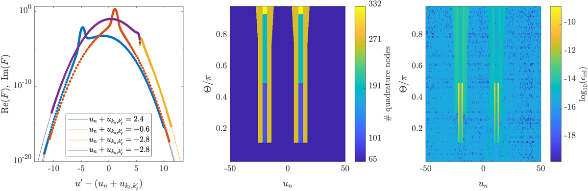
Illustrative examples of the quadrature grids. Left: real part (blue and red lines) and positive and negative values of the imaginary part (yellow and purple lines, respectively) of F as a function of $u^{\prime }-\left(u_n+u_{k_{\ell },k_{\ell }^{\prime }}\right)$, with u′ = u(ν′), u_n = u(ν_n), and $u_{k_{\ell },k_{\ell }^{\prime }}=u_{k_u,k_{\ell }^{\prime }}-u_{k_u,k_{\ell }}$, for different values of $u+u_{k_u,k_{\ell }^{\prime }}$. Here, a = 0.01, Θ = 0.9π, $u_{k_u,k_{\ell }}=-11.1$, and $u_{k_u,k_f^{\prime }}=-11.2$. The dots denote the quadrature nodes u_n′ generated with u^∗ = −11.15. Centre: number of quadrature nodes as a function of u_n and Θ, with a = 0.01, $u_1^{\ast }=-11.15$, and $u_2^{\ast }=20$. Right: logarithm of the relative error of evaluating Eq. (11) with the quadrature nodes of the central panel with respect to the reference values obtained with the Gauss–Kronrod adaptive method, with I = (1, 0, 0, 0), a = 0.01, and $u_{k_u,k_{\ell }}=u_{k_u,k_{\ell }^{\prime }}=-11.1$.