| Issue |
A&A
Volume 628, August 2019
|
|
|---|---|---|
| Article Number | A6 | |
| Number of page(s) | 22 | |
| Section | Interstellar and circumstellar matter | |
| DOI | https://doi.org/10.1051/0004-6361/201935200 | |
| Published online | 25 July 2019 | |
The physical and chemical structure of Sagittarius B2
IV. Converging filaments in the high-mass cluster forming region Sgr B2(N)
1
I. Physikalisches Institut, Universität zu Köln,
Zülpicher Strasse 77,
50937
Köln,
Germany
e-mail: schwoerer@ph1.uni-koeln.de
2
National Radio Astronomy Observatory,
1003 Lopezville Rd.,
Socorro,
NM
87801,
USA
3
Max-Planck-Institut für extraterrestrische Physik,
Gießenbachstraße 1,
85748
Garching bei München,
Germany
4
Jet Propulsion Laboratory, California Institute of Technology,
4800 Oak Grove Drive,
Pasadena,
CA
91109,
USA
5
Sorbonne Université, Observatoire de Paris, Université PSL, CNRS, LERMA,
75005
Paris,
France
6
Department of Astronomy, Yunnan University, and Key Laboratory of Astroparticle Physics of Yunnan Province,
Kumming
650091,
PR China
Received:
4
February
2019
Accepted:
22
April
2019
Context. Sagittarius B2 (north) is a chemically rich, high-mass star-forming region located within the giant molecular cloud complex Sgr B2 in the central molecular zone of our Galaxy. Dust continuum emission at 242 GHz, obtained at high angular resolution with the Atacama Large Millimeter Array (ALMA), reveals that it has a filamentary structure on scales of 0.1 pc.
Aims. We aim to characterize the filamentary structure of Sgr B2(N) and its kinematic properties using multiple molecular dense gas tracers.
Methods. We have used an unbiased, spectral line-survey that covers the frequency range from 211 to 275 GHz and obtained with ALMA (angular resolution of 0.′′4, or 3300 au) to study the small-scale structure of the dense gas in Sgr B2(N). In order to derive the kinematic properties of the gas in a chemically line-rich source like Sgr B2(N), we have developed a python-based tool that stacks all the detected line transitions of any molecular species. This allows us to increase the signal-to-noise ratio (S/N) of our observations and average out line blending effects, which are common in line-rich regions.
Results. A filamentary network is visible in Sgr B2(N) in the emission maps of the molecular species CH3OCHO, CH3OCH3, CH3OH and H2CS. In total, eight filaments are found that converge to the central hub (with a mass of 2000 M⊙, assuming a temperature of 250 K) and extending for about 0.1 pc (up to 0.5 pc). The spatial structure, together with the presence of the massive central region, suggest that these filaments may be associated with accretion processes, transporting material from the outer regions to the central dense hub. We derive velocity gradients along the filaments of about 20–100 km s−1 pc−1, which are 10–100 times larger than those typically found on larger scales (~1 pc) in other star-forming regions. The mass accretion rates of individual filaments are ≾0.05 M⊙ yr−1, which result in a total accretion rate of 0.16 M⊙ yr−1. Some filaments harbor dense cores that are likely forming stars and stellar clusters. We determine an empirical relation between the luminosity and stellar mass of the clusters. The stellar content of these dense cores is on the order of 50% of the total mass. The timescales required for the dense cores to collapse and form stars, exhausting their gas content, are compared with the timescale of their accretion process onto the central hub. We conclude that the cores may merge in the center when already forming stellar clusters but still containing a significant amount of gas, resulting in a “damp” merger.
Conclusions. The high density and mass of the central region, combined with the presence of converging filaments with high mass, high accretion rates and embedded dense cores already forming stars, suggest that Sgr B2(N) may have the potential to evolve into a super stellar cluster.
Key words: stars: formation / stars: massive / techniques: high angular resolution / ISM: kinematics and dynamics / ISM: individual objects: SgrB2(N) / radio lines: ISM
© ESO 2019
1 Introduction
The star-forming complex Sagittarius B2 (hereafter Sgr B2) is the most massive cloud in our Galaxy with a mass of 107 M⊙ and H2 densities of 103–105 cm−3 (Schmiedeke et al. 2016; Hüttemeister et al. 1995; Goldsmith et al. 1990), located at a distance1 of 8.127± 0.031 kpc (Gravity Collaboration 2018) in the vicinity of the Galactic center (at a projected distance of 107 pc) within the central molecular zone (CMZ). The CMZ provides an extreme environment in terms of pressure, turbulent Mach number, and gas temperature (~60 to >100 K), which are much higher than those found in star-forming regions distributed throughout the Galactic disk (Ginsburg et al. 2016; Morris & Serabyn 1996), but comparable to the physical conditions found in starburst galaxies. Therefore, the CMZ and Sgr B2 are perfect targets to study star formation under extreme conditions in our local environment. The complex Sgr B2 harbors two main sites of active high-mass star formation, Sgr B2 Main (M) and North (N), with masses of 104 –105 M⊙ and H2 densities of ~107 cm−3. Moreover, active high-mass star formation and a huge number of different (complex) molecules have been observed in both of them (e.g. De Pree et al. 2014; Belloche et al. 2013; Schmiedeke et al. 2016; Sánchez-Monge et al. 2017; Ginsburg et al. 2018; Mills et al. 2018). We have begun a project characterizing the physical and chemical properties of Sgr B2 covering all the spatial scales from au up to tens of parsec. For this, we combined multiwavelength observationswith 3D radiative transfer modeling (see Schmiedeke et al. 2016; Sánchez-Monge et al. 2017; Pols et al. 2018). In this paper, the fourth of the series, we make use of high-spatial resolution observations obtained with ALMA2 (0.′′4, or 3300 au) to studythe small-scale structure of the dense gas in Sgr B2(N). The dust continuum emission studied in Sánchez-Monge et al. (2017, herafter Paper II) revealed a filamentary network converging to a central hub, which has a total mass of about 2000 M⊙ (assuming a temperature of 250 K) and densities ~109 cm−3. In this paper, we characterized the kinematic properties of the filaments in more detail by making use of the molecular line emission observed with ALMA. Filaments have been found, in part thanks to the Herschel satellite, to be ubiquitous entities in molecular clouds at many different scales. Their presence in almost all the environments suggest that they play an important role during the early phasesof the star formation process. It has been found in local low-mass star forming regions at scales of a few pc that filaments are hatcheries of prestellar cores (e.g. Taurus B211/B213, Palmeirim et al. 2013; Marsh et al. 2016). Similarly, molecular clouds forming high-mass stars (O and B spectral type stars) are found to be pervaded by large and complex filamentary networks, when observed at large scales of a few pc (see e.g. Orion: Suri et al. 2019; Hacar et al. 2018; MonR2: Treviño-Morales et al. 2019). In these cases, stellar clusters are found to form in dense hubs with densities >106 cm−3. Denser high-mass star forming regions like W33A (~107–108 cm−3), when observed with high enough angular resolution, show filamentary structures at scales of a few 1000 au and converging toward the most massive objects forming in the clusters (Maud et al. 2017; Izquierdo et al. 2018). Sgr B2(N) provides us, thanks to the high densities of 108 –109 cm−3, with an ideal target to characterize filaments in even more extreme environments. Moreover, the high densities and masses found in the central region of Sgr B2(N) suggest that this region may evolve into a super stellar cluster or young massive cluster (YMC), similar to the Arches and Quintuplet clusters. YMCs are considered to be predecessors of globular clusters, which are formed at the earliest epochs of the universe. Their formation process is still poorly understood, in particular, the mechanism of mass accumulation, during which filaments may play an important role. This paper is structured as follows. In Sect. 2 we describe our ALMA observations. In Sect. 3 we present the physical and kinematic properties of the filaments found in Sgr B2(N). In Sect. 4 we discuss our results of the converging filaments and argue that Sgr B2(N) may form a super stellar cluster. Finally, in Sect. 5 we summarize the main results.
2 ALMA observations
In June 2014 and June 2015, Sgr B2 was observed with ALMA (Atacama Large Millimeter/submillimeter Array) during its Cycle 2. 34–36 antennas were used in an extended configuration with baselines in the range from 30 to 650 m, which provided an angular resolution of 0.′′3–0.′′7. The chosen spectral scan mode surveyed the whole ALMA band 6 (211–275 GHz) with 10 different spectral tunings, providing a spectral resolution of 0.5–0.7 km s−1. Sgr B2(N), with phase center at α(J2000) = 17h 47m19s.887, δ(J2000) = −28°22′15.′′76, was observed in track-sharing mode together with Sgr B2(M). The calibration and imaging processes were carried out with CASA3 version 4.4.0. All the images were restored with a common Gaussian beam of 0.′′4. Further details of the observations, calibration, and imaging are provided in Paper II.
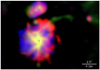 |
Fig. 1 Three-color composite image of Sgr B2(N). The green image shows the continuum emission at 242 GHz (Paper II), the red image corresponds to the molecular species CH3 OCHO, and the blue image to C2H5CN. The center, which is dominated by the continuum and CH3OCHO emission, appears yellow. The images of the molecular species have been constructed from stacked cubes (see more details in Sect. 3 and Appendix A) and correspond to peak intensity maps. The continuum emission and species like CH3 OCHO trace a filamentary structure, while species such as C2H5CN show a spherical or bubble-like shape. The white circle indicates the position of the central core with coordinates α(J2000) = 17h47m19s.87, δ(J2000) = −28°22′18.′′43. |
3 Filamentary structure in Sgr B2(N)
The line survey toward Sgr B2(N) revealed an extremely rich chemistry in many of the compact sources reported in Paper II, with more than 100 lines per GHz. While the detailed chemistry is the subject of another study (Möller et al., in prep.), in the current work we focus on species with bright and clearly identified4 transitions. Among them, S-bearing species like H2CS and OCS, N-bearing species like CH3CN and C2H5CN, and O-bearing species like CH3OH, CH3OCHO and CH3OCH3. We used themost isolated lines of these molecular species and produced peak intensity maps. These maps reveal two main types of structures which are illustrated in Fig. 1. The dust continuum emission at 242 GHz (see Paper II) and species like CH3OCH3 (dimethyl ether), CH3OCHO (methyl formate), CH3OH, 13CH3OH (methanol) and H2CS (thioformaldehyde) show a filamentary structure (green and red in Fig. 1), whereas other molecules like C2 H5CN (ethylcyanid) or OCS (carbonylsulfid) trace instead a spherical or bubble-like shape (blue in Fig. 1). The existence of two different morphologies in different molecular species hints at opacity effects, excitation conditions or chemical variations as possible origins. Opacity effects are most likely to be discarded, because we detect a large number of species including rare isotopologues (i.e. less affected by opacity effects) tracing both structures. The chemical and excitation properties of both structures will be discussed in a forthcoming paper (Schwörer et al., in prep). Here, we have focussed on the four molecular species CH3OCHO, CH3OCH3, CH3OH, and 13CH3OH included in the spectral-line survey that trace the filamentary structure and study its kinematic properties. The analysis of spectral-line surveys with thousands of lines is challenging because of line blending effects of known and unknown molecular species, particularly in a chemically-rich region like Sgr B2. For any single transition it is thus not straightforward to accurately determine its spatial distribution and the kinematic properties (e.g., velocity, linewidth, lineshape). However, taking advantage of the existence of 100s of lines for each species, we developed a tool that stacks all transitions of a certain molecule. Line stacking improves the signal-to-noise ratio (S/N), as well as averaging out line blendings. This permits us to derive the real spatial distribution of the molecular species, as well as the true line shape and number of (velocity) components. A more detailed description of the method is presented in Appendix A. We used the stacked data cubes for different species to characterize the properties of the filaments in Sgr B2(N).
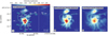 |
Fig. 2 Panel a: map of the ALMA 242 GHz continuum emission of Sgr B2(N). The white dots indicate the position of the continuum sources reported in Paper II. The green dashed lines trace the path of the filaments identified inthe molecular line data (see Sect. 3.1), while gray dashed lines trace tentative elongated structures not clearly confirmed in the molecular emission maps. The light-gray circles indicate H II regions (see De Pree et al. 2014, and Paper I). Panel b: peak intensity map of the bright, isolated transition of CH3OCHO at 229.404 GHz. Panel c: peak intensity map of the bright H2CS transition at 244.048 GHz. In all panels, the synthesized beam of 0.′′4 is shown in the bottom-left corner, and a spatial scale bar is shown in the bottom-right corner. |
3.1 Filament identification and properties
The identification of the filaments has been done tracing their peak intensity, starting at a position close to the dense hub and following the intensity ridge outwards by visual inspection. Since the central region is optically thick and most lines appear in absorption against the bright continuum, we exclude this region. We used peak intensity maps created from stacked cubes (see Appendix A), because their higher S/N allow for a better determination of faint structures. The identified filaments were also confirmed in peak intensity maps created from individual molecular transitions. In total, we identify eight arms or filaments (see Fig. 2) which are visible in emission of different species. While arms F01, F03, F04, F05, F06, F07, and F08 emit in the molecules CH3OCH3, CH3OCHO, CH3OH and 13CH3OH, arm F02 is only visible in H2CS. Arm F08 is the most extended and seems to connect the central hub with regions located ~ 0.5 pc to the west. However, the outer (western) part is mainly visible in continuum and not in molecular lines which prevents an analysis of its velocity structure (see Sect. 4). This arm leads to a chalice-shaped area (cf. bright red emission in Fig. 1) when approaching the central hub, and contains the dense cores A04, A05, A07 (from Paper II), and the H II region H02 (De Pree et al. 2014). On the contrary, filament F07 appears the shortest, probably due to strong projection effects. Some filaments (F01, F05, F06, and F08) harbor embedded cores, while others appear more homogeneous and without clear hints of fragmentation along them, suggesting the existence of different physical conditions (Schwörer et al., in prep.). The northern satellite core (containing dense cores A02, A03, and A06, and being one of the main targets in the search of complex molecular species, e.g. Belloche et al. 2013) seems to be connected by arms F01 and F02 to the main hub (see Sect. 4 for further detail). However, arm F01 seems broken, maybe caused by feedback of the neighbor H II region H01. The area to the southwest, in between filaments F05 and F07 looks disordered, and the possibility of another underneath filament can not be excluded (see gray dashed lines in Fig. 2, see also Fig. 1).
3.2 Filament kinematics
The analysis of the velocity structure of each filament has been done using the stacked cubes, excluding arm F02 which is only visible in H2 CS. This molecule has, in the frequency range of our line survey, only four transitions, thus the statistical method of line-stacking offers no significant advantages. The peak velocity map of the stacked transitions of CH3OCHO (see Fig. 3) reveals already a clear velocity gradient from red to blue-shifted velocities between the northern satellite core and the main hub. Overall, we see a smooth velocity structure, except at the interface between the northern and main cores, where several velocity components are present. A more detailed study of the velocity structure is obtained by producing position-velocity (pv) cuts along the filaments and by fitting Gaussian functions to the spectra. In Appendix B we show the pv-cuts for different molecular species. Most of the filaments are well described by a single velocity component, with the exception of filament F06, for which we consider two velocity components. The Gaussian fits of each spectrum along the filament allow us to derive the velocity and linewidth of each species, and better explore possible variations with distance along the filaments (see Appendix D). For all the filaments, we see velocity gradients in all four species, and we fit them with a linear function. In Table 1, we list the velocity gradients of seven filaments for three species. The velocity structure of each filament is consistent between different molecular species, suggesting that these species trace gas with similar kinematic properties. We determine an average velocity gradient of roughly 20 km s−1 pc−1. Arm F07 reaches the highest values of 52–70 km s−1 pc−1, which together with its short length, suggests that F07 is a filament oriented close to the line of sight. While the gradients in filaments F04, F05, and F06 are negative, meaning that they go from red to blue-shifted velocities when moving from the main hub outwards, the gradients in filament F03 and F07 are positive. The pv-cut along the most extended filament F08 shows a connection in its velocity structure between the main hub and the far away western dense cores A15 located at a distance of ~0.27 pc and A08/A09 located at a distance of ~0.5 pc (see Fig. 4). The kinematic structure of some filaments shows clear variations in the trend of their velocity structure (see e.g. F03, F08, Fig. D.1, and Fig. D.2). This is likely due to the filaments not being perfect straight lines, but having some curvature in the 3D space, which may result in different velocity gradients (along the filaments) when seen in projection. We used these variations to define subsections (labeled with roman numbers) along these filaments (see Appendix D). We divide filament F03 in two sections from 0.02 to 0.055 pc, and 0.07 to 0.12 pc, and filament F08 in three sections from 0.01 to 0.04 pc, 0.055 to 0.07 pc, and 0.08 to 0.11 pc. Filament F01 has a weak additional velocity component, best visible in CH3OH (see Fig. C.1), but also in CH3OCHO, connecting the northern satellite core with the main hub. We divided F01 into three sections from 0 to 0.03 pc, 0.032 to 0.11 pc, and 0.115 to 0.018 pc. Moreover, as discussed above (see also Fig. C.1), F06 has two velocity components in the range 0–0.04 pc, that we labeled as F06a and F06b. In addition to the velocity gradient derived for each filament as a single entity, we calculate the velocity gradient for every identified segment (see Table 1). In Fig. 5 (top panel), we present an overview of the velocity gradients of each filament and subfilament. The variation of the velocity linewidth along the filament for each species is shown in Fig. D.3, while the mean linewidths, evaluated as the average Gaussian width along the filament, are shown in Fig. 5 (middle panel). Typical linewidths range from 3 to 8 km s−1, with a decreasing trend when moving from the central hub outwards. Along filaments F03, F04, F05, and F08, the linewidth of CH3OCHO and 13 CH3OH behave quite similar, while the linewidth of CH3OH is in most cases twice the linewidth of the other species. This is further studied in a forthcoming paper (Schwörer et al., in prep.). Filament F05 has a local linewidth minimum at ~0.075 pc, coincident with the position of another filament, which is not unambiguously identified in our current data (see Fig. 2 and Sect. 3.1).
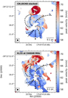 |
Fig. 3 Peak velocity map of H2CS (bottom-panel) and CH3OCHO (top-panel, using 143 stacked lines, see Appendix A). The emission below 10σ and the center are masked out. The filaments and position of dense cores are marked with black dashed lines and white dots, respectively. |
Kinematic and physical properties of the filaments in Sgr B2(N).
 |
Fig. 4 Position velocity cut along filament F08 in CH3OCHO and H2 CS. The emission to the left corresponds to the filament close to the central hub. The emission at about 0.25 pc and 0.4 pc corresponds to the cores A15 and A08, A19. The white dashed line corresponds to a velocity gradient of ~16 km s−1 pc−1, consistent with the mean velocity gradient of F08 (see Table 2). |
3.3 Massaccretion rates and filament stability
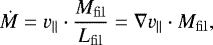
We evaluated the mass accretion rate of each filament using its mass and the derived velocity gradients. The mass of each filament was estimated from the dust continuum emission at 242 GHz (see Paper II). For optically thin emission, a dust opacity of 0.899 cm2 g−1 (Ossenkopf & Henning 1994), a dust-to-gas mass ratio of 100, and dust temperatures between 50 and 100 K, we derive masses of the filaments in the range 200–1000 M⊙ (see Table 1). The higher mass values for filaments F01 and F08 are due to the elongation of F01 into the central hub and thepresence of the bright chalice-shaped structure surrounding F08. Since filaments F03 and F04 are located close together in the plane of the sky, part of their mass might be double-counted, although the effect should be negligible, since the overlap of the filaments occurs only in about one fourth of their extend. Following Kirk et al. (2013), we calculate the mass accretion rate implied by our velocity gradients assuming a cylindrical model for our filaments. The mass accretion rate (Ṁ) is derived as
 (1)
(1)
where Mfil is the mass of the filament, Lfil the length of the filament and v|| the velocity parallel to the filament. Considering an inclination α between the filament and the plane of the sky, the parameters that we observe are given by
 (2)
(2)
which modify the mass accretion rate to
 (3)
(3)
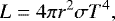
For the calculation of the mass accretion rates, we assumed a projection angle α of 45°. An angle of 25° roughly doubles our results, while an angle of 65° halves them. For the velocity gradient, we used the median of the values determined for all the species (see Table 1). In Fig. 5 (bottom panel), we plot the mass accretion rates for all the filaments and subfilaments. The mass accretion rates along the filaments of Sgr B2(N) are between 0.004 and 0.04 M⊙ yr−1 at the scales of 0.1–0.2 pc (see Table 1), thus 10–100 times largerthan rates usually found in star-forming filaments at larger scales of ~1 pc (e.g., Peretto et al. 2013; Lu et al. 2018; Treviño-Morales et al. 2019). Altogether, considering the average accretion rates listed in Table 1, the filaments in Sgr B2(N) accrete at a rate of 0.08–0.16 M⊙ yr−1. This results in a total of 80–160 M⊙ accreted onto the dense hub in about 1000 yr, suggesting a timescale for the formation of the hub of about 60–300 kyr, assuming current accretion rates. In Sect. 3.1, we show that some filaments appear fragmented and harbor embedded cores, which raises the question of how stable the filaments are. The mass-to-length ratio (M/L) is a measure of the stability of the filament (e.g., Ostriker 1964; Fischera & Martin 2012). If this value exceeds a critical limit, the filament will gravitationally collapse under its weight perpendicular to its main axis. Assuming that turbulence can stabilize the filament, the critical value is calculated as
 (4)
(4)
where σ is the velocity dispersion and G the gravitational constant. Since the measured linewidths are in the range of 3–8 km s−1 (see Fig. 5), we can neglect the thermal contribution, which corresponds to a few 0.1 km s−1 for the considered species at 50–100 K. This results in a value of  about (4–30) × 103 M⊙ pc−1. According to our measured mass-to-length ratio (see Table 1), the filaments in Sgr B2(N) seem to be stable under gravitational collapse. The variation of M/L along the filaments by assuming different temperatures is presented in Fig. G.1 and show a decreasing trend when moving from the central hub outwards.
3.4 Dense core properties and accretion timescales
We determined the temperatures of the dense cores (from Paper II) located within the filaments by fitting the spectral lines of different molecular species with the software XCLASS (Möller et al., in prep.). All values are in the range of 50–200 K and listed in Table 2. These high temperatures suggest the presence of already formed stars inside the cores5. The stellar content can be derived from the luminosity of the dense cores. Considering them as spherical black bodies, the stellar luminosity is given by the Stefan–Boltzmann equation
 (5)
(5)
where r is the radius of the dense cores, σ the Stefan–Boltzmann constant and T the temperature. We present more details regarding the black body assumption and the validity of the Stefan–Boltzmann law in Appendix E. The derived luminosities are listed in Table 2. The large gas masses of the dense cores (see Paper II and Table 2) suggest that not one single star, but a stellar cluster is forming in each core. While the relation between stellar mass and luminosity is known for single stars (e.g., Eker et al. 2018), there is no direct relation for star clusters. Thus, we have simulated 105 clusters, and determined the final stellar luminosity and mass (see Appendix F for details). We find that the cluster luminosity and stellar mass of a cluster follow the relation
 (6)
(6)
The stellar mass content, Mstellar, for each core within the filaments is listed in Table 2. With this, we calculated the ratio between the stellar mass and total mass as
 (7)
(7)
All values are summarized in Table 2 and visualized in Fig. 6. For all cores, the stellar mass is within the range 20–90% of the total mass, with a mean (median) value of 50% (44%). We have also investigated the relation of the mass of the different cores with respect to their distance to the central hub. In Fig. 7, we plot the core mass (top panel) and the stellar mass ratio (bottom panel) as a function of the distance to the hub. While no striking correlation is found, we see a bimodal distribution. Cores with masses above 200 M⊙ are located preferentially at distances <0.25 pc, while less massive cores can be found up to distances of about 0.5 pc. Similarly, cores located closer to the central hub can have a higher stellar mass fraction than those located farther away. In Sect. 4.2 we discuss these results in the context of converging filaments and the formation of a cluster in Sgr B2(N). One further question of interest is whether the dense cores will be accreted onto the central hub before they are disrupted by internal star formation. The timescale for forming stars can be estimated by assuming that the dense cores will collapse on a free-fall timescale
 (8)
(8)
where M is the mass of the dense core and r its radius (values reported in Paper II). The tcore,ff values are listed in the last column of Table 2, and range from 103 to 104 yr. We compared the tcore,ff with the time required by the dense cores to travel from their position to the central dense hub assuming a free-fall scenario along the filaments, tfil,ff (see Table 2). To estimate the gravitational acting central mass (see Eq. (8)), we integrated the flux density over the entire dense hub and assume an averaged temperature of 50–100 K that result, in a mass between (25 and 10) × 103 M⊙. The distance is given by the separation between the core and the central hub. The tfil,ff ranges from 103 to 104 yr, comparable to the timescale over which a core collapses and forms a stellar cluster.
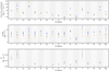 |
Fig. 5 Overview picture of the velocity gradients (top panel), velocity linewidths (middle panel) and mass accretion rates (bottom panel) along all filaments and subfilaments (indicated by roman numbers) in Sgr B2(N), see Sects. 3.1 and 3.2. Additional velocity components in filament F06 are marked as 6a and 6b. The gray, green, blue, and orange symbols correspond to the molecules CH3OCHO, CH3OCH3, CH3OH and 13CH3OH, respectively. |
Properties and timescales of the dense cores located within filaments in Sgr B2(N).
 |
Fig. 6 Stellar mass fraction (see Sect. 3.4) of the dense cores. Cores are grouped by their host filaments. |
4 Discussion
4.1 Converging filaments
The analysis of transitions of different molecular species reve- aled a network of filaments in Sgr B2(N), converging toward a central massive core. We derived velocity gradients along the filaments, which are 10–100 times larger than is usually found in other star-forming regions at larger scales (e.g. Peretto et al. 2013; Lu et al. 2018). We have considered here if these large velocity gradients can be caused by other mechanisms rather than accretion to the center, for example expanding motions associated with outflows or explosive events like the one seen in Orion KL (e.g. Bally et al. 2017). For outflows, typical linewidths are 30–100 km s−1 (e.g. Wu et al. 2004; López-Sepulcre et al. 2010; Sánchez-Monge et al. 2013), roughly ten times larger than what we measure. Furthermore, common outflow tracers are CO, HCO+ and SiO (e.g. Wu et al. 2004; Sánchez-Monge et al. 2013; but see also Palau et al. 2011, 2017) and not complex molecules like CH3OCHO or CH3OCH3 which we find tracing the filamentary structure of Sgr B2(N). Explosion events such as that in Orion KL are also a doubtful explanation since they produce clear and straightforward radial structures. Contrary to this, the structures that we identified in Sgr B2(N) appear curved and bent, which leaves us with accreting filaments as the most plausible explanation. For cylindrical, spatially tilted filaments, the transport of material along them toward the dense hub (i.e. velocities close to the center are higher than outwards) would result in different signs of the velocity gradient, as we find in Sgr B2(N) (see Fig. 5 and Table 1). In this scenario, positive velocity gradients correspond to filaments extending backwards, and vice-versa, allowing us to have an idea of the possible 3D structure of the region. In Fig. 8 we show the distribution of filaments in Sgr B2(N) colored by velocity gradient, in which red corresponds to positive velocity gradients (filaments located in the back) and blue to negative velocity gradients (filaments located in front). A remarkable case in Sgr B2(N) are the neighboring filaments F03 and F04. Filament F03 would be located in the back while F04 in front of the hub. Overall, filaments F03, F07, and F08 would be located in the back, and F04, F05, and F06 would be in front (see Fig. 8). In addition to the velocity field, we find that the linewidths for many filaments (e.g. F01, F03, F05, F06, and F08, see Fig. D.3) increase when approaching the center6. This effect, combined with the increasing mass-to-length ratio (derived independently from the continuum emission) when moving inwards, suggests that the accretion or infall rates onto the filaments may be increasing in the vicinity of the main hub.
Finally, some filaments appear extended, connecting multiple dense cores with the main hub. In particular, filament F08 extends up to the distant western cores A08 and A19, located at distances ~0.5 pc. Although the molecular line emission is not bright in the filament between core A05 and cores A08 and A19, the velocity in A19 fits the velocity gradient obtained in the region of the filament closer to the hub (see Fig. 4). This suggests that these cores, even if being far away, are connected to the central hub. Similarly, the northern core seems to be connected to the main hub trough filaments F01 and F02. Despite filament F01 being affected by the H II region H01, the emission of CH3OH reveals, through a second velocity component, a link between the northern core and the hub (see Fig. C.1). Filament F02, which is only visible in the emission of H2CS, shows a smooth velocity gradient from highly red to blue-shifted velocities when moving from the northern core to the central hub (see Fig. C.2). This suggests that the distant cores as well as the northern core may fall onto the hub, increasing the gas and stellar density, and favoring Sgr B2(N) to become a super stellar cluster.
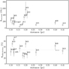 |
Fig. 7 Top panel: total mass of the dense cores against their distance to the main hub. Bottom panel: Stellar mass fraction of the densecores against their distance to the main hub. The gray dashed line indicates the mean stellar mass fraction of of 50%. |
 |
Fig. 8 Filaments in Sgr B2(N) colored by their mean velocity gradient as derived for the molecular species CH3OCHO, CH3OCH3, CH3OH and 13CH3OH. The velocity gradient ranges from −50 km s−1 pc−1 (blue), corresponding to filaments located in front, to +50 km s−1 pc−1 (red), corresponding to filaments located in the back. The gray contours indicating 242 GHz continuum emission at a level of 1.2 Jy beam−1. The white circles represent the dense cores, and the black dashed line shows the filament F02, only visible in H2 CS. |
4.2 High-mass cluster formation
The high densities found in Sgr B2(N) (109 cm−3, or 107 M⊙ pc−1, see Paper II), the large mass reservoir of the envelope, and high star formation activity in a number of dense cores suggest that Sgr B2(N) may gather enough mass to form a super-stellar cluster or young massive cluster (YMC), therefore constituting a good candidate YMC progenitor. The formation of YMCs is still poorly understood, and different scenarios have been proposed (e.g. Portegies Zwart et al. 2010; Longmore et al. 2014 for a review, and Bressert et al. 2012; Fujii 2015; Fujii & Portegies Zwart 2016; Howard et al. 2019). The “in situ formation” scenario proposes that the required amount of gas mass is gathered into the same volume of the final stellar cluster before star formation sets in. The extreme densities required to form a YMC, entail that the accumulated gas has a short free-fall time, which in turn implies that the time for gathering the final mass has to be short or, alternatively, the star formation activity is delayed until the accumulation of the total mass. In a second scenario, the “conveyor belt formation” theory proposes that the mass reservoir extends farther away than the final stellar cluster size. Thus, stars can form in regions with much lower densities and be transported toward the center of the cluster, increasing the final density of the YMC. Our analysis of the properties of Sgr B2(N) suggests a mix of the two scenarios. On one side, the dense cores located within the filaments already harbor stars, according to our simulations in the ballpark of 2000 (see Appendix F), before merging into the main hub. This supports the idea of the conveyor belt models (“dry” merger), in which star forming clusters are transported throughout the filaments toward the center of the region. On the other hand, the stellar mass ratio is 50%, that is, the dense cores are still surrounded by dense gas while reaching the central region. Although our statistics are small, we see the trend that dense cores located closer to the central hub can be more massive than in the outer regions, (see Fig. 7) suggesting that they have acquired more mass on their way to the main hub. In addition, the comparison of timescales listed in Table 2 suggests that the dense cores can reach the center before they have exhausted all the gas to form stars. Finally, the measured high mass accretion rates (0.08–0.16 M⊙ yr−1) point to a short time necessary to accumulate a large mass reservoir, as proposed by the in-situ (“wet” merger) formation scenarios. Assuming constant accretion rates, the central dense hub, with (25–10) × 103 M⊙, has been assembled in only 60–300 kyr. However, the fraction of stars is large (~ 50%) compared to the amount of gas mass in the cores. As a result we cannot consider this process as a clear wet merger, but as a “damp” merger. Overall, Sgr B2(N) has the potential to become a YMC or super stellar cluster similar to the Arches and Quintuplet clusters, which are also located in the CMZ near the Galactic center.
5 Summary
We have studied the spatial distribution and kinematic properties of a number of molecular species detected in the high-mass star-forming region Sgr B2(N). We used ALMA observations with an angular resolution of 0.′′4 (corresponding to 3300 au) and covering the frequency range from 211 to 275 GHz. The rich chemistry of Sgr B2(N) results in the detection of thousands of lines, often overlapping and therefore difficult to analyze. In order to overcome this problem, we have developed a python-based tool that stacks lines of any given molecular species resulting in an increase of the final S/N and averaging out line blending effects. This has permitted us to study the distribution of the molecular emission and its kinematic properties. Our main results are summarized in the following:
-
We have identified two different spatial structures related to the molecular emission in Sgr B2(N). Molecular species like CH3OCH3, CH3OCHO, CH3OH, or H2CS show a filamentary network similar to the distribution of the dust continuum emission at 242 GHz. Contrary to that, species like OCS or C2H5CN show a spherical or bubble-like distribution that will be further analyzed in forthcoming papers.
-
We haveidentified eight filaments, which converge toward the central massive core or hub. All but one filament are traced inmultiple molecules, including rare isotopologues. Filament F02 is detected in our dataset in only one molecule, H2CS. The filaments extent for about 0.1 pc (some up to 0.5 pc) and have masses of a few hundred M⊙. The structure and distribution of the filaments, together with the presence of a massive central region (~2000 M⊙), suggest that these filaments play an important role in the accretion process and transport mass from the outer regions to the central hub.
-
From theline emission, we measure velocity gradients along the filaments on the order of 20–100 km s−1 pc−1 at scales of ~0.1 pc. This is 10–100 times larger than typical velocity gradients found in other star forming regions at larger scales (~1 pc). We derive mass accretion rates in individual filaments of up to 0.05 M⊙ yr−1, which add to a total of 0.16 M⊙ yr−1 when considering the accretion of all the filaments into the central hub.
-
The dense cores identified in the 242 GHz continuum emission map are found distributed along these filaments. We have determined the stellar mass content of these cores, and compare the timescale for the dense cores to collapse and form stars or clusters, with the timescale required for them to be accreted onto the central hub. Considering simple approximations, the free-fall timescale for the core collapse is longer than the time of accretion onto the hub. This suggests that although stars and clusters can form within the cores while being accreted, they will not exhaust all the gas. This is consistent with the stellar mass fractions of 50% (with respect to the total mass) that we derive. This suggests a scenario of a damp merger Sgr B2(N).
-
In summary, Sgr B2(N) contains a central hub with large densities (~ 109 cm−3, or 107 M⊙ pc−3), a series of massive dense cores (~200 M⊙) with the potential to form stellar clusters, and a network of filaments converging toward a central hub, with large velocity gradients and high mass accretion rates (up to 0.16 M⊙ yr−1). The large mass already contained in the central hub (~2000 M⊙ in about 0.05 pc size) together with the merging process of dense cores already harboring stellar clusters, suggest that Sgr B2(N) has the potential to become a super stellar cluster like the Arches or Quintuplet clusters.
Acknowledgements
This work was supported by the Deutsche Forschungsgemeinschaft (DFG) through grant Collaborative Research Centre 956 (subproject A6 and C3, project ID 184018867) and from BMBF/Verbundforschung through the projects ALMA-ARC 05A11PK3 and 05A14PK1. This paper makes use of the following ALMA data: ADS/JAO.ALMA#2013.1.00332.S. ALMA is a partnership of ESO (representing its member states), NSF (USA) and NINS (Japan), together with NRC (Canada) and NSC and ASIAA (Taiwan) and KASI (Republic of Korea), in cooperation with the Republic of Chile. The Joint ALMA Observatory is operated by ESO, AUI/NRAO and NAOJ. DCL acknowledges support of the Scientific Council of the Paris Observatory. Part of this research was carried out at the Jet Propulsion Laboratory, California Institute of Technology, under a contract with the National Aeronautics and Space Administration. In order to do the analysis and plots, we used the python packages scipy, numpy, pandas, matplotlib, astropy, aplpy and seaborn.
Appendix A Line stacking method
The analysis of line-rich surveys with often thousands of lines has its pitfalls due to an unknown number of spectral line components and blending of multiple species. Particularly, deriving velocity information is therefore rather complicated in line-crowded spectra. In chemically rich regions like Sgr B2, it is not easily possible to identify well isolated transitions, which are usable to determine the kinematic structure. Moreover, large velocity gradients across the observed region as well as different chemical compositions throughout the source are obstructive. In spite of these adversities, we convert the difficulty of the presence of innumerable lines within a blind survey into an advantage. For this, we have developed an automatized (python based) tool to stack all transitions of a certain species to increase the S/N and to average out line blending effects. The process of stacking is commonly used in Astronomy to increase the S/N of for example, weak radio galaxies, recombination lines and even faint molecular line transitions (see e.g., Beuther et al. 2016; Lindroos et al. 2015; Loomis et al. 2018). In our case, stacked data also simplifies the structure and shape of the spectral lines, thus making it possible to analyze the velocity and kinematic properties. The method is carried out in three main steps, illustrated in Fig. A.1. First (step A in the figure), we correct our observed data by the source LSR velocity, corresponding to about 64 km s−1 for Sgr B2(N). Subsequently, we produce a synthetic spectrum with XCLASS (Möller et al. 2017) for any molecular species assuming similar conditions (i.e., temperatures, column densities) to those representing the region (Möller et al., in prep.). An accurate fit of the observed data to derive the best temperature, column densities and velocities is helpful but not mandatory. Reasonable assumptions are enough to determine which frequency transitions are detected in the observations, since the synthetic spectrum is used for the identification of bright transitions. For example, for the case of CH3OCHO, we identified 250 bright lines above a 10σ threshold in the frequency range 211 to 275 GHz. This selection prevents us from including transitions that are included in the catalog entries of the CDMS and JPL databases, but are too weak and most likely non detected, in our source of interest. Moreover, the exclusion of the weak transitions, reduces the addition of components highly dominated by noise or by the presence of (bright) transitions from other species. Second (step B in Fig. A.1), we cut out all the identified transitions and produce subspectra centered at them. These spectra are transformed from frequency to velocity by applying the Doppler equation. The velocity at 0 km s−1 (see Fig. A.1) corresponds to the rest frequency listed in the database, since we have corrected the data by the source LSR velocity. The spectra are uniformly resampled and rebined, using the python packages signal and numpy, to ensure that the channels in the velocity frame have the same width. Finally (step C in Fig. A.1), all spectra are averaged by taking the arithmetic mean. In the final stacked spectra, the S/N has increased, while at the same time line blendings are averaged out. This simplifies ensuing the analysis of the kinematic properties like velocity, linewidth, lineshape or number of components. The stacking process can be applied to a subsample of transitions, selected for example, by excitation energy level (Eupper) or Einstein A coefficient, parameters included in the molecular line databases CDMS and JPL. This selection of transitions will be used in a forthcoming paper to characterize the excitation and physical conditions of the filaments in Sgr B2(N). We performed tests with synthetic spectra to demonstrate the reliability of the line stacking method. We have used the XCLASS software to generate a synthetic spectrum of the molecular species C2 H3CN (Acrylonitrile), which is a good candidate since it has approximately 300 clearly detectable transitions in the observed frequency range (211–275 GHz). The synthetic spectrum of C2 H3CN is produced including two different velocity components with velocities of 0 and − 5 km s−1, and linewidths of 4 and 2 km s−1. In Fig. A.2, we show the results. In the top panel we have stacked the transitions of the synthetic spectrum. The stacked spectrum shows a clear two-velocity component profile. We fit Gaussian distributions and recover the velocities and linewidths with an accuracy of 98%. In a second run (see Fig. A.2, bottom panel) we combine the synthetic spectrum with the observed data of Sgr B2(N). We note that the molecule C2 H3CN is not detected in our data and therefore the only transitions that should be found are those include in the synthetic spectrum. After performing line stacking, we recovered the velocities of the two components with a high accuracy (about 98%). The derived linewidths are slightly larger than the original ones, resulting in an accuracy of 82%. This increase in the linewidth is likely produced by the presence of neighboring transitions of other molecular species, which act like noise and result in the broadening effect. Therefore, line-stacking of chemically rich regions results in slightly broader lines. We also note that the presence of this additional transitions artificial increases the continuum level, while not affecting the velocity information of the lines.
 |
Fig. A.1 Line stacking process for molecular lines in a spectral survey. Step A: correct observed spectrum, shown in black in the top, by the source LSR velocity (corresponding to 64 km s−1 for Sgr B2(N)). Create a synthetic spectrum (shown in red, and using XCLASS) for the considered molecular species. This will beused for the identification of detectable transitions (highlighted with a gray shadow area). Step B: extract a portion of the spectrum centered at each transition, and transform the frequency axis into velocity using the Doppler equation. Each cutout spectra is uniformly resampled and rebined. Step C: sum up all the cutout spectra and divide by the number of transitions. Normalization has been waived to prevent that noise and lines from other molecular species are not scaled up. Line blendings are statistically averaged out and the true line shape and the velocity can be determined. |
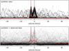 |
Fig. A.2 Accuracy check of the line stacking method. Upper panel: stacking performed with a pure synthetic spectrum of the molecular species C2H3CN. The velocity and velocity width have been fully recovered. Lower panel: stacking of the same synthetic spectrum combined with observed data. The line velocity stays recoverable with high precision, while the velocity width has slightly increased but in a negligible order. |
Appendix B Peak intensity maps
In Fig. B.1 we present peak intensity maps of selected transitions of different molecular species. The path of the filaments is overlaid on all of them. The filamentary structures are clearly visible in molecular species CH3OCHO, CH3OCH3, CH3OH, and 13CH3OH. For other species such as C2 H5CN and OCS, the bubble-shape structure dominates the emission.
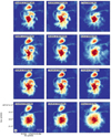 |
Fig. B.1 Peak intensity maps of transitions of various molecular species showing either the filamenary structure or bubble shape. The green dashed lines trace the path of the filaments identified in the stacked data (see Sect. 3.1). |
Appendix C Position-velocity plots along the filaments
Figure C.1 shows the position-velocity plots produced along the main spines of the filaments as depicted in Fig. 2. We have used the stacked cubes of the molecular species CH3OCHO, CH3OCH3, CH3OH and 13CH3OH, shown in gray, green, blue, and orange, respectively. The position-velocity plots are obtained following a similar approach to what is implemented in the python tool pvextractor, and considering an averaging width across the filament of 0.′′4, corresponding to the synthesized beam. Similarly, Fig. C.2 shows the position-velocity plot along filament F02, which is only visible in H2 CS.
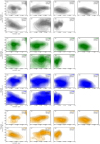 |
Fig. C.1 Position-velocity plots along each filament, for the molecules CH3OCHO (gray), CH3OCH3(green), CH3OH (blue), and 13CH3OH (orange), from top to bottom. |
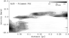 |
Fig. C.2 Position velocity cut along filament F02 in H2CS. The emission to the left corresponds to the filament close to the central hub. The emission at about 0.27 pc corresponds to the northern satellite core. |
Appendix D Velocity gradients and linewidth variation
In order to constrain the velocity properties, we fit Gaussian functions to the spectra along the filaments to study the variation of velocity and linewidth. In Figs. D.1 and D.2 (right panels), we plot the variation of velocity with distance, while in Fig. D.3, we plot the variation of the linewidth (see Sect. 3 for a discussion on the kinematic properties of the filaments). As discussed in Sect. 3.2, all filaments show velocity gradients in the molecular species CH3OCHO, CH3OCH3, CH3OH and 13CH3OH. We study the variation of the velocity gradient along the filament by performing linear fits in 0.014 pc size sections (corresponding to 0.′′4, or a beam size) along the filament. The distribution of the velocity gradients are shown in the left panels of Figs. D.1 and D.2 in the form of violin plots, which are a combination of box plots and a kernel density plot. The distribution of velocity gradients for the different filaments has, in most cases, a dominant peak, which is generally in agreement with the average velocity gradient determined for the whole filament (listed in Table 1). The second components in the distributions confirm the presence more than one velocity gradient value along the filaments, suggesting acomplex velocity gradient structure which could be due to curvatures and projection effects in the filaments.
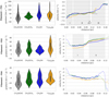 |
Fig. D.1 Left panels: distribution of velocity gradients along the filaments (determined in sections of 0.014 pc) shown in form of a violin plot. The outer (or violin) shape represents all possible velocity gradients, with broadening indicating how common they are, meaning that the broadest part represents the mode average. The black thin bar indicates all datapoints in the violin interior, while its thicker part corresponds to the quartiles of the distribution, with the white dot indicating the mean value of all velocity gradients along the respective filament. The distribution is shown for the molecules CH3OCHO, CH3OCH3, CH3OH and 13CH3OH. Right panel: velocity variation along the filaments. The gray areas indicate subsections along the filaments, labeled with roman numbers. The position of the dense cores are indicatedby vertical, black dashed lines. Regions where the line emission is below 4σ are plotted with dashed lines. |
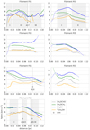 |
Fig. D.3 Variation of the line width along the filaments. The position of the dense cores are indicated by vertical, black dashed lines. Sections for which the line emission is below 4σ are plotted with dashed lines. |
Appendix E Blackbody assumption
We derived the stellar luminosity of the dense cores assuming that they are spherical black bodies and we use the Stefan–Boltzmann law. However, these dense cores are not perfect black bodies, and the dust opacity has to be taken into account. The modified blackbody or Planck function is
 (E.1)
(E.1)
where Bν(T) is the Planck function at temperature T and τν is the optical depth at frequency ν, which is proportional to the density along the line of sight, given by
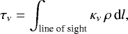 (E.2)
(E.2)
with κν being the absorption coefficient (opacity) per unit of total mass density and ρ the density. We modeled the modified Planck function for different hydrogen column densities  between 1020 –1025 cm−2 and a temperature of 100 K (see Fig. E.1). The absorption coefficients are taken from Ossenkopf & Henning (1994) according to dust grains with thin ice mantles and gas densities of 106 cm−3. We assume a dust-to-gas mass ratio of 100. The total brightness of an emitting source can be obtained by integrating over the (modified) Planck function
 (E.3)
(E.3)
For a perfect black body, this results in
 (E.4)
(E.4)
where σ is the Stefan–Boltzmann constant. The luminosity calculated from a numerical integration over the Planck function and multiplied by a spherical surface of a given radius matches the luminosity calculated with the Stefan–Boltzmann law. For a more detailed derivation see Wilson et al. (2009). In Fig. E.2, we present the ratio between the brightness of a perfect black body and a modified black body as function of the column density. For hydrogen densities above roughly 5 × 1023 cm−2, the total brightness obtained for a modified Planck function is in agreement with the brightness of a perfect black body, with deviations of less than 6%. At the observed high column densities, the emission is optically thick already at lower frequencies compared to lower column densities (see deviations from the Planck function in Fig. E.1), and the variation in the total integrated brightness is not significant. In Sgr B2(N) we have column densities about 1024 cm−2 (Sánchez-Monge et al. 2017). Hence, the assumption of a blackbody is reasonable and the luminosity, which is proportional to the total brightness, can be calculated with the Stefan–Boltzmann law (see Eq. (5)).
 |
Fig. E.1 Modified Planck function for different column densities from 1020 to 1025 cm−2 at a temperature of 100 K. The solid gray curves are calculated based on the opacities of Ossenkopf & Henning (1994), while the dashed lines are obtained from the extrapolation of the two lowest frequency values in Ossenkopf & Henning (1994). The Planck function or perfect black body at a temperature of 100 K is shown with a black solid and thick line. |
 |
Fig. E.2 Ratio between the total brightness of the modified Planck function and a perfect blackbody. The gray dots marked the ratio for specific column densities, while the dashed lines show the trend. The hatched area indicates the range of column densities found in the dense cores of Sgr B2(N). |
Appendix F Stellar luminosity and mass relation for clusters
In order to determine the stellar mass and luminosity of clusters, we simulated 105 clusters with a random amount of stars. The number of stars varies between 1 and 50 000, with masses from 0.1 to 100 M⊙. The mass distribution of stars for each cluster follows the Initial Mass Function (IMF; Kroupa 2001),
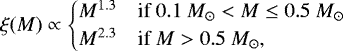 (F.1)
(F.1)
where ξ is the number of stars of a certain mass. The stellar luminosity (L) for a given star of mass M follows the relation (see Eker et al. 2018)
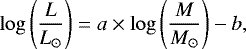 (F.2)
(F.2)
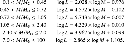
where the constants a and b vary depending on the stellar mass. For the range of masses considered, we use (based on Eker et al. 2018):
The masses and luminosities of all individual stars are summed, and result in a total mass and luminosity per cluster. The result for all simulated clusters is shown in Fig. F.1, presenting the relation between the stellar mass of the cluster and the cluster luminosity. In Fig. F.2, we show the relation between  and the cluster luminosity. We fit a linear function to the relation and find
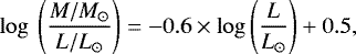 (F.3)
(F.3)
where M is the mass of the cluster and L the cluster luminosity. In the particular case of the cores of Sgr B2(N), we determine the stellar mass of the clusters that form inside by making use of the luminosities listed in Table 2. For this, we extract all the simulated clusters with luminosities corresponding to the core luminosity, within a range of ±10%. The stellar mass distributions of the selected clusters are shown as histograms in Fig. F.3 We finally determined the stellar mass Mstellar as the median value of the distribution. We note that the number of stars within the dense cores of Sgr B2(N) is found to be below 2000 objects (see also Fig. F.1)
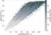 |
Fig. F.1 Relation between the stellar mass and stellar luminosity for clusters with different numbers of stars. The white contours show the 2D kernel density estimate (KDE) of the simulated clusters. |
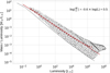 |
Fig. F.2 Relation between the ratio |


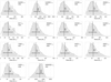 |
Fig. F.3 Stellar mass distribution of clusters with luminosities according to the observed dense cores in Sgr B2(N). The gray line shows the KDE obtained with the python package seaborn. The black dashed vertical lines indicate the mean values of the mass distribution, and the horizontal lines indicate the standard deviation. |
Appendix G Mass-to-length ratio
In Fig. G.1 we plot the variation of mass-to-length ration along the filament. The mass has been computed for segments of 0.011 pc in length and for three different dust temperatures: 50, 100, and 300 K. Taking the 50 K case as an example, we find for all filaments an increase of mass when approaching the center of the region. This may be due to a higher mass content in the inner regions of the filaments. Alternatively, this might be an artifact produced by a wrong temperature assumption. If the filament is hotter in the inner regions (e.g., six times hotter, from50 to 300 K) the increase in mass toward the center is less significant, although still existing in many filaments.
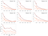 |
Fig. G.1 Variation of mass-to-length ratio (M/L) along the filaments, computed along sections of 0.011 pc in length. The different lines correspond to different assumed temperatures: 50 (dark), 100 (orange), and 300 K (light orange). |
References
- ALMA Partnership, Fomalont, E. B., Vlahakis, C., et al. 2015, ApJ, 808, L1 [Google Scholar]
- André, P., Men’shchikov, A., Bontemps, S., et al. 2010, A&A, 518, L102 [NASA ADS] [CrossRef] [EDP Sciences] [Google Scholar]
- Arzoumanian, D., André, P., Didelon, P., et al. 2011, A&A, 529, L6 [Google Scholar]
- Bally, J., Ginsburg, A., Arce, H., et al. 2017, AJ, 837, 60 [Google Scholar]
- Belloche, A., Müller, H. S. P., Menten, K. M., Schilke, P., & Comito, C. 2013, A&A, 559, A47 [NASA ADS] [CrossRef] [EDP Sciences] [Google Scholar]
- Beuther, H., Bihr, S., Rugel, M., et al. 2016, A&A, 595, A32 [NASA ADS] [CrossRef] [EDP Sciences] [Google Scholar]
- Bressert, E., Ginsburg, A., Bally, J., et al. 2012, ApJ, 758, L28 [NASA ADS] [CrossRef] [Google Scholar]
- De Pree, C. G., Peters, T., Mac Low, M.-M., et al. 2014, ApJ, 781, L36 [NASA ADS] [CrossRef] [Google Scholar]
- Eker, Z., Bakış, V., Bilir, S., et al. 2018, MNRAS, 479, 5491 [NASA ADS] [CrossRef] [Google Scholar]
- Endres, C. P., Schlemmer, S., Schilke, P., Stutzki, J., & Müller, H. S. P. 2016, J. Mol. Spectr., 327, 95 [NASA ADS] [CrossRef] [Google Scholar]
- Fischera, J., & Martin, P. G. 2012, A&A, 542, A77 [NASA ADS] [CrossRef] [EDP Sciences] [Google Scholar]
- Fujii, M. S. 2015, PASJ, 67, 59 [NASA ADS] [CrossRef] [Google Scholar]
- Fujii, M. S., & Portegies Zwart S. 2016, ApJ, 817, 4 [NASA ADS] [CrossRef] [Google Scholar]
- Ginsburg, A., Henkel, C., Ao, Y., et al. 2016, A&A, 586, A50 [NASA ADS] [CrossRef] [EDP Sciences] [Google Scholar]
- Ginsburg, A., Bally, J., Barnes, A., et al. 2018, ApJ, 853, 171 [NASA ADS] [CrossRef] [Google Scholar]
- Goldsmith, P. F., Lis, D. C., Hills, R., & Lasenby, J. 1990, ApJ, 350, 186 [NASA ADS] [CrossRef] [Google Scholar]
- Gravity Collaboration (Abuter R., et al.) 2018, A&A, 615, L15 [NASA ADS] [CrossRef] [EDP Sciences] [Google Scholar]
- Hacar, A., Tafalla, M., Forbrich, J., et al. 2018, A&A, 610, A77 [NASA ADS] [CrossRef] [EDP Sciences] [Google Scholar]
- Howard, C. S., Pudritz, R. E., Harris, W. E., & Sills, A. 2019, MNRAS, 486, 1146 [NASA ADS] [CrossRef] [Google Scholar]
- Hüttemeister, S., Wilson, T. L., Mauersberger, R., et al. 1995, A&A, 294, 667 [NASA ADS] [Google Scholar]
- Izquierdo, A. F., Galván-Madrid, R., Maud, L. T., et al. 2018, MNRAS, 478, 2505 [NASA ADS] [CrossRef] [Google Scholar]
- Kirk, H., Myers, P. C., Bourke, T. L., et al. 2013, ApJ, 766, 115 [NASA ADS] [CrossRef] [Google Scholar]
- Kroupa, P. 2001, MNRAS, 322, 231 [NASA ADS] [CrossRef] [Google Scholar]
- Lindroos, L., Knudsen, K. K., Vlemmings, W., Conway, J., & Martí-Vidal, I. 2015, MNRAS, 446, 3502 [NASA ADS] [CrossRef] [Google Scholar]
- Longmore, S. N., Kruijssen, J. M. D., Bastian, N., et al. 2014, Protostars and Planets VI (Tucson: University of Arizona Press), 291 [Google Scholar]
- Loomis, R. A., Öberg, K. I., Andrews, S. M., et al. 2018, AJ, 155, 182 [NASA ADS] [CrossRef] [Google Scholar]
- López-Sepulcre, A., Cesaroni, R., & Walmsley, C. M. 2010, A&A, 517, A66 [NASA ADS] [CrossRef] [EDP Sciences] [Google Scholar]
- Lu, X., Zhang, Q., Liu, H. B., et al. 2018, ApJ, 855, 9 [NASA ADS] [CrossRef] [Google Scholar]
- Marsh, K. A., Kirk, J. M., André, P., et al. 2016, MNRAS, 459, 342 [NASA ADS] [CrossRef] [Google Scholar]
- Maud, L. T., Hoare, M. G., Galván-Madrid, R., et al. 2017, MNRAS, 467, L120 [NASA ADS] [Google Scholar]
- McMullin, J. P., Waters, B., Schiebel, D., Young, W., & Golap, K. 2007, Astronomical Data Analysis Software and Systems XVI, 376, 127 [NASA ADS] [Google Scholar]
- Mills, E. A. C., Ginsburg, A., Clements, A. R., et al. 2018, ApJ, 869, L14 [NASA ADS] [CrossRef] [Google Scholar]
- Möller, T., Endres, C., & Schilke, P. 2017, A&A, 598, A7 [NASA ADS] [CrossRef] [EDP Sciences] [Google Scholar]
- Morris, M., & Serabyn, E. 1996, ARA&A, 34, 645 [NASA ADS] [CrossRef] [Google Scholar]
- Müller, H. S. P., Thorwirth, S., Roth, D. A., & Winnewisser, G. 2001, A&A, 370, L49 [NASA ADS] [CrossRef] [EDP Sciences] [Google Scholar]
- Müller, H. S. P., Schlöder, F., Stutzki, J., et al. 2005, IAU Symp., 235, 62 [Google Scholar]
- Ossenkopf, V., & Henning, T. 1994, A&A, 291, 943 [NASA ADS] [Google Scholar]
- Ostriker, J. 1964, ApJ, 140, 1529 [NASA ADS] [CrossRef] [Google Scholar]
- Palau, A., Fuente, A., Girart, J. M., et al. 2011, ApJ, 743, L32 [NASA ADS] [CrossRef] [Google Scholar]
- Palau, A., Walsh, C., Sánchez-Monge, Á., et al. 2017, MNRAS, 467, 2723 [NASA ADS] [Google Scholar]
- Palmeirim, P., André, P., Kirk, J., et al. 2013, A&A, 550, A38 [NASA ADS] [CrossRef] [EDP Sciences] [Google Scholar]
- Peretto, N., Fuller, G. A., Duarte-Cabral, A., et al. 2013, A&A, 555, A112 [NASA ADS] [CrossRef] [EDP Sciences] [Google Scholar]
- Pickett, H. M. 1991, J. Mol. Spectr., 148, 371 [NASA ADS] [CrossRef] [Google Scholar]
- Pols, S., Schwörer, A., Schilke, P., et al. 2018, A&A, 614, A123 [NASA ADS] [CrossRef] [EDP Sciences] [Google Scholar]
- Portegies Zwart, S. F., McMillan, S. L. W., & Gieles, M. 2010, ARA&A, 48, 431 [NASA ADS] [CrossRef] [Google Scholar]
- Reid, M. J., Menten, K. M., Brunthaler, A., et al. 2014, ApJ, 783, 130 [Google Scholar]
- Sánchez-Monge, Á., López-Sepulcre, A., Cesaroni, R., et al. 2013, A&A, 557, A94 [NASA ADS] [CrossRef] [EDP Sciences] [Google Scholar]
- Sánchez-Monge, Á., Beltrán, M. T., Cesaroni, R., et al. 2014, A&A, 569, A11 [NASA ADS] [CrossRef] [EDP Sciences] [Google Scholar]
- Sánchez-Monge, Á., Schilke, P., Schmiedeke, A., et al. 2017, A&A, 604, A6 (Paper II) [NASA ADS] [CrossRef] [EDP Sciences] [Google Scholar]
- Schmiedeke, A., Schilke, P., Möller, T., et al. 2016, A&A, 588, A143 (Paper I) [NASA ADS] [CrossRef] [EDP Sciences] [Google Scholar]
- Suri, S. T., Sanchez-Monge, A., Schilke, P., et al. 2019, A&A, 623, A142 [NASA ADS] [CrossRef] [EDP Sciences] [Google Scholar]
- Treviño-Morales, S. P., Fuente, Á., Sánchez-Monge, A., et al. 2019, A&A, accepted [arXiv:1907.03524] [Google Scholar]
- Wilson, T. L., Rohlfs, K., & Hüttemeister, S. 2009, Tools of Radio Astronomy (Berlin, Germany: Springer-Verlag) [Google Scholar]
- Wu, Y., Wei, Y., Zhao, M., et al. 2004, A&A, 426, 503 [NASA ADS] [CrossRef] [EDP Sciences] [Google Scholar]
For consistency with previous findings in the literature, for our calculations we used the distance 8.34 ± 0.16 kpc (Reid et al. 2014).
Atacama Large Millimeter/submillimeter Array, ALMA Partnership et al. (2015).
The Common Astronomy Software Applications (CASA; McMullin et al. 2007). Downloaded at http://casa.nrao.edu
The assignment of transitions to molecular species is done using the software XCLASS: eXtended CASA Line Analysis Software Suite: Möller et al. (2017), which make uses of the Cologne Database for Molecular Spectroscopy (CDMS, Müller et al. 2001, 2005) and Jet Propulsion Laboratory (JPL, Pickett 1991) catalogs, via the Virtual Atomic and Molecular Data Centre (VAMDC, Endres et al. 2016).
Other mechanisms such as external or shock heating can be excluded. For a typical density of 106 cm−3 and temperature of 100 K, a heating source would need to see the core as optically thin around the peak (~30 μm) of the black body emission. The dust absorption coefficient κν at 30 μm is about 300 cm2 g−1, which yields a distance of only 50 au. Therefore, the heating source has to be effectively embedded in order to heat the gas to the measured temperatures. Heating through shocks is also unlikely since for infall rates of ≤0.16 M⊙ yr−1 and a assumed accretion shock velocity of ~8 km s−1, the derived luminosities are only 1700 L⊙, less than the average luminosities derived for our cores.
We note that the increase of linewidth toward the center may be partially caused by the line stacking method. The positions along the filament close to the center show a richer chemistry (i.e., more line features). This excess of lines, compared to the outer positions, may result in a artificial increase of the linewidth (see Appendix A for further detail).
All Tables
Properties and timescales of the dense cores located within filaments in Sgr B2(N).
All Figures
|
Fig. 1 Three-color composite image of Sgr B2(N). The green image shows the continuum emission at 242 GHz (Paper II), the red image corresponds to the molecular species CH3 OCHO, and the blue image to C2H5CN. The center, which is dominated by the continuum and CH3OCHO emission, appears yellow. The images of the molecular species have been constructed from stacked cubes (see more details in Sect. 3 and Appendix A) and correspond to peak intensity maps. The continuum emission and species like CH3 OCHO trace a filamentary structure, while species such as C2H5CN show a spherical or bubble-like shape. The white circle indicates the position of the central core with coordinates α(J2000) = 17h47m19s.87, δ(J2000) = −28°22′18.′′43. |
| In the text | |
|
Fig. 2 Panel a: map of the ALMA 242 GHz continuum emission of Sgr B2(N). The white dots indicate the position of the continuum sources reported in Paper II. The green dashed lines trace the path of the filaments identified inthe molecular line data (see Sect. 3.1), while gray dashed lines trace tentative elongated structures not clearly confirmed in the molecular emission maps. The light-gray circles indicate H II regions (see De Pree et al. 2014, and Paper I). Panel b: peak intensity map of the bright, isolated transition of CH3OCHO at 229.404 GHz. Panel c: peak intensity map of the bright H2CS transition at 244.048 GHz. In all panels, the synthesized beam of 0.′′4 is shown in the bottom-left corner, and a spatial scale bar is shown in the bottom-right corner. |
| In the text | |
|
Fig. 3 Peak velocity map of H2CS (bottom-panel) and CH3OCHO (top-panel, using 143 stacked lines, see Appendix A). The emission below 10σ and the center are masked out. The filaments and position of dense cores are marked with black dashed lines and white dots, respectively. |
| In the text | |
|
Fig. 4 Position velocity cut along filament F08 in CH3OCHO and H2 CS. The emission to the left corresponds to the filament close to the central hub. The emission at about 0.25 pc and 0.4 pc corresponds to the cores A15 and A08, A19. The white dashed line corresponds to a velocity gradient of ~16 km s−1 pc−1, consistent with the mean velocity gradient of F08 (see Table 2). |
| In the text | |
|
Fig. 5 Overview picture of the velocity gradients (top panel), velocity linewidths (middle panel) and mass accretion rates (bottom panel) along all filaments and subfilaments (indicated by roman numbers) in Sgr B2(N), see Sects. 3.1 and 3.2. Additional velocity components in filament F06 are marked as 6a and 6b. The gray, green, blue, and orange symbols correspond to the molecules CH3OCHO, CH3OCH3, CH3OH and 13CH3OH, respectively. |
| In the text | |
|
Fig. 6 Stellar mass fraction (see Sect. 3.4) of the dense cores. Cores are grouped by their host filaments. |
| In the text | |
|
Fig. 7 Top panel: total mass of the dense cores against their distance to the main hub. Bottom panel: Stellar mass fraction of the densecores against their distance to the main hub. The gray dashed line indicates the mean stellar mass fraction of of 50%. |
| In the text | |
|
Fig. 8 Filaments in Sgr B2(N) colored by their mean velocity gradient as derived for the molecular species CH3OCHO, CH3OCH3, CH3OH and 13CH3OH. The velocity gradient ranges from −50 km s−1 pc−1 (blue), corresponding to filaments located in front, to +50 km s−1 pc−1 (red), corresponding to filaments located in the back. The gray contours indicating 242 GHz continuum emission at a level of 1.2 Jy beam−1. The white circles represent the dense cores, and the black dashed line shows the filament F02, only visible in H2 CS. |
| In the text | |
|
Fig. A.1 Line stacking process for molecular lines in a spectral survey. Step A: correct observed spectrum, shown in black in the top, by the source LSR velocity (corresponding to 64 km s−1 for Sgr B2(N)). Create a synthetic spectrum (shown in red, and using XCLASS) for the considered molecular species. This will beused for the identification of detectable transitions (highlighted with a gray shadow area). Step B: extract a portion of the spectrum centered at each transition, and transform the frequency axis into velocity using the Doppler equation. Each cutout spectra is uniformly resampled and rebined. Step C: sum up all the cutout spectra and divide by the number of transitions. Normalization has been waived to prevent that noise and lines from other molecular species are not scaled up. Line blendings are statistically averaged out and the true line shape and the velocity can be determined. |
| In the text | |
|
Fig. A.2 Accuracy check of the line stacking method. Upper panel: stacking performed with a pure synthetic spectrum of the molecular species C2H3CN. The velocity and velocity width have been fully recovered. Lower panel: stacking of the same synthetic spectrum combined with observed data. The line velocity stays recoverable with high precision, while the velocity width has slightly increased but in a negligible order. |
| In the text | |
|
Fig. B.1 Peak intensity maps of transitions of various molecular species showing either the filamenary structure or bubble shape. The green dashed lines trace the path of the filaments identified in the stacked data (see Sect. 3.1). |
| In the text | |
|
Fig. C.1 Position-velocity plots along each filament, for the molecules CH3OCHO (gray), CH3OCH3(green), CH3OH (blue), and 13CH3OH (orange), from top to bottom. |
| In the text | |
|
Fig. C.2 Position velocity cut along filament F02 in H2CS. The emission to the left corresponds to the filament close to the central hub. The emission at about 0.27 pc corresponds to the northern satellite core. |
| In the text | |
|
Fig. D.1 Left panels: distribution of velocity gradients along the filaments (determined in sections of 0.014 pc) shown in form of a violin plot. The outer (or violin) shape represents all possible velocity gradients, with broadening indicating how common they are, meaning that the broadest part represents the mode average. The black thin bar indicates all datapoints in the violin interior, while its thicker part corresponds to the quartiles of the distribution, with the white dot indicating the mean value of all velocity gradients along the respective filament. The distribution is shown for the molecules CH3OCHO, CH3OCH3, CH3OH and 13CH3OH. Right panel: velocity variation along the filaments. The gray areas indicate subsections along the filaments, labeled with roman numbers. The position of the dense cores are indicatedby vertical, black dashed lines. Regions where the line emission is below 4σ are plotted with dashed lines. |
| In the text | |
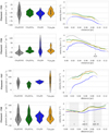 |
Fig. D.2 Same as Fig. D.1 for filaments F05, F06, F07 and F08. |
| In the text | |
|
Fig. D.3 Variation of the line width along the filaments. The position of the dense cores are indicated by vertical, black dashed lines. Sections for which the line emission is below 4σ are plotted with dashed lines. |
| In the text | |
|
Fig. E.1 Modified Planck function for different column densities from 1020 to 1025 cm−2 at a temperature of 100 K. The solid gray curves are calculated based on the opacities of Ossenkopf & Henning (1994), while the dashed lines are obtained from the extrapolation of the two lowest frequency values in Ossenkopf & Henning (1994). The Planck function or perfect black body at a temperature of 100 K is shown with a black solid and thick line. |
| In the text | |
|
Fig. E.2 Ratio between the total brightness of the modified Planck function and a perfect blackbody. The gray dots marked the ratio for specific column densities, while the dashed lines show the trend. The hatched area indicates the range of column densities found in the dense cores of Sgr B2(N). |
| In the text | |
|
Fig. F.1 Relation between the stellar mass and stellar luminosity for clusters with different numbers of stars. The white contours show the 2D kernel density estimate (KDE) of the simulated clusters. |
| In the text | |
|
Fig. F.2 Relation between the ratio |
| In the text | |
|
Fig. F.3 Stellar mass distribution of clusters with luminosities according to the observed dense cores in Sgr B2(N). The gray line shows the KDE obtained with the python package seaborn. The black dashed vertical lines indicate the mean values of the mass distribution, and the horizontal lines indicate the standard deviation. |
| In the text | |
|
Fig. G.1 Variation of mass-to-length ratio (M/L) along the filaments, computed along sections of 0.011 pc in length. The different lines correspond to different assumed temperatures: 50 (dark), 100 (orange), and 300 K (light orange). |
| In the text | |
Current usage metrics show cumulative count of Article Views (full-text article views including HTML views, PDF and ePub downloads, according to the available data) and Abstracts Views on Vision4Press platform.
Data correspond to usage on the plateform after 2015. The current usage metrics is available 48-96 hours after online publication and is updated daily on week days.
Initial download of the metrics may take a while.