| Issue |
A&A
Volume 693, January 2025
|
|
|---|---|---|
| Article Number | A160 | |
| Number of page(s) | 18 | |
| Section | Interstellar and circumstellar matter | |
| DOI | https://doi.org/10.1051/0004-6361/202451274 | |
| Published online | 14 January 2025 | |
The physical and chemical structure of Sagittarius B2
VIII. Full molecular line survey of hot cores
1
I. Physikalisches Institut, Universität zu Köln,
Zülpicher Str. 77,
50937
Köln,
Germany
2
Institut de Ciències de l’Espai (ICE, CSIC),
Campus UAB, Carrer de Can Magrans s/n,
08193
Bellaterra, Barcelona,
Spain
3
Institut d’Estudis Espacials de Catalunya (IEEC),
08860
Castelldefels, Barcelona,
Spain
4
Green Bank Observatory,
155 Observatory Rd,
Green Bank,
WV
24944,
USA
★ Corresponding author; This email address is being protected from spambots. You need JavaScript enabled to view it.
Received:
26
June
2024
Accepted:
20
November
2024
Abstract
Context. The giant molecular cloud complex Sagittarius B2 (Sgr B2) in the central molecular zone of our Galaxy hosts several high-mass star formation sites, with Sgr B2(M) and Sgr B2(N) being the main centers of activity. This analysis aims to comprehensively model each core spectrum, considering molecular lines, dust attenuation, and free-free emission interactions. We describe the molecular content analysis of each hot core and identify the chemical composition of detected sources.
Aims. Using ALMA’s high sensitivity, we aim to characterize the hot core population in Sgr B2(M) and N, gaining a better understanding of the different evolutionary phases of star formation processes in this complex.
Methods. We conducted an unbiased ALMA spectral line survey of 47 sources in band 6 (211-275 GHz). Chemical composition and column densities were derived using XCLASS, assuming local thermodynamic equilibrium. Quantitative descriptions for each molecule were determined, considering all emission and absorption features across the spectral range. Temperature and velocity distributions were analyzed, and derived abundances were compared with other spectral line surveys.
Results. We identified 65 isotopologs from 41 different molecules, ranging from light molecules to complex organic compounds, originating from various environments. Most sources in the Sgr B2 complex were assigned different evolutionary phases of high-mass star formation.
Conclusions. Sgr B2(N) hot cores show more complex molecules such as CH3OH, CH3OCHO, and CH3OCH3, while M cores contain lighter molecules such as SO2, SO, and NO. Some sulfur-bearing molecules are more abundant in N than in M. The derived molecular abundances can be used for comparison and to constrain astrochemical models. Inner sources in both regions were generally more developed than outer sources, with some exceptions.
Key words: ISM: clouds / dust, extinction / evolution / ISM: molecules / ISM: individual objects: Sagittarius B2(M) / ISM: individual objects: Sagittarius B2(N)
© The Authors 2025
 Open Access article, published by EDP Sciences, under the terms of the Creative Commons Attribution License (https://creativecommons.org/licenses/by/4.0), which permits unrestricted use, distribution, and reproduction in any medium, provided the original work is properly cited.
This article is published in open access under the Subscribe to Open model. This email address is being protected from spambots. You need JavaScript enabled to view it. to support open access publication.
1 Introduction
With a mass of 107 M⊙ and H2 densities of 103−105 cm−3 (Schmiedeke et al. 2016; Hüttemeister et al. 1995; Lis & Goldsmith 1989), Sagittarius B2 (Sgr B2) is one of the most massive molecular clouds in our Galaxy. Sgr B2 is part of the central molecular zone (CMZ, Henshaw et al. 2023). It is located at a distance1 of 8.178 ± 0.013stat. ± 0.022sys. kpc (GRAVITY Collaboration 2019) and is situated at a projected distance of 107 pc from Sgr A*, the compact radio source associated with the supermassive black hole in the Galactic center.
The Sgr B2 complex contains two main sites of active high- mass star formation, Sgr B2 Main (M) and North (N), which are separated by ~48″ (~1.9 pc in projection). With comparable luminosities of 2−10 × 106 L⊙, masses of 5 × 10⁴ M⊙, and sizes of ~0.5 pc (see Schmiedeke et al. 2016) these two sites are located at the center of an envelope with a radius of 2 pc, which contains at least ~70 high-mass stars with spectral types in the range from O5 to B0 (see e.g., Gaume et al. 1995; De Pree et al. 2014). All of this together is embedded in another envelope with a radius of 20 pc, which contains more than 99% of the total mass of Sgr B2. Compared to Sgr B2(N), Sgr B2(M) shows a higher degree of fragmentation, has a higher luminosity, and contains more ultracompact H II regions (see e.g., Goldsmith et al. 1992; Qin et al. 2011; Sánchez-Monge et al. 2017; Schwörer et al. 2019; Meng et al. 2019), which suggests a more evolved stage and larger amount of feedback. Moreover, previous studies show that M is very rich in sulfur-bearing molecules, while N is dominated by organics (Sutton et al. 1991; Nummelin et al. 1998; Friedel et al. 2004; Belloche et al. 2013; Neill et al. 2014). The complex and multilayered structures of high-mass proto-clusters such as Sgr B2 are difficult to study. The high density of molecular lines and the continuum emission detected toward the two main sites indicate the presence of a large amount of material to form new stars. Spectral line studies provide the opportunity to gain a better insight into their thermal excitation conditions and dynamics by examining line intensities and profiles, allowing for the separation of different physical components and identification of chemical patterns. Additionally, line surveys offer the possibility to study the distribution of exciting sources by looking at vibrationally excited molecules. Since IR radiation is needed to excite them (e.g., Costagliola & Aalto 2010), they should delineate the exact position of the exciting sources, which are otherwise difficult to see due to extinction even at millimeter wavelengths.
Although Sgr B2 has been the target of numerous spectral line surveys before (see e.g., Cummins et al. 1986; Turner 1989; Sutton et al. 1991; Nummelin et al. 1998; Friedel et al. 2004; Belloche et al. 2013, 2016, 2019; Neill et al. 2014, Möller et al. 2021), the unique capabilities of the Atacama Large Millime- ter/submillimeter Array (ALMA) now offer further insight into the process of star formation. Hot cores have been identified as birthplaces of high-mass stars where the central protostar(s) heats up the surrounding dense envelope. These regions are compact (diameters ≤0.1 pc), dense (n ≥ 107 cm−3), hot (T ≥100 K), and dark (Av ≥ 100 mag) molecular cloud cores (see e.g., van der Tak 2004). The high temperatures of the hot cores lead to the sublimation of icy dust mantles, which are the main sites for the formation of complex organic molecules. Additionally, the molecular line emission in hot cores provides powerful constraints on both the physical and chemical conditions in these regions (Kurtz et al. 2000; Bisschop et al. 2007). Although many hot cores show similarities in their molecular content, they possess a great diversity in terms of relative molecular abundances (see e.g., Walmsley & Schilke 1993; Bisschop et al. 2007; Belloche et al. 2013; Minh et al. 2018). Furthermore, hot cores are often associated with outflows, infall, and rotation. In later stages of the hot cores, ultracompact H II regions (UCH II) are formed, where the protostars ionize their surrounding envelope.
In this paper, which continues our series of studies on Sgr B2 (Schmiedeke et al. 2016; Sánchez-Monge et al. 2017; Pols et al. 2018; Schwörer et al. 2019; Meng et al. 2019; Meng et al. 2022; Möller et al. 2023), we describe the full analysis of broadband spectral line surveys of hot cores, identified by Sánchez-Monge et al. (2017) in Sgr B2(M) and N, to characterize the hot core population in the Sgr B2 complex, where we take the complex interactions between molecular lines, dust attenuation, and free-free emission arising from H II regions into account. In the first half of our analysis, described in the seventh paper of our series on the analysis of the Sgr B2 complex, Paper VII (Möller et al. 2023), we have quantified the dust and, if contained, the free-free contributions to the continuum levels of each core, and we have derived the corresponding parameters not only for each core but also for their local surrounding envelope, and determined their physical properties. In this paper, we describe the analysis of the molecular content of each hot core and identify the chemical composition of the detected sources.
This paper is laid out as follows. We start with Sect. 2, where we describe the observations and outline the data reduction procedure, followed by Sect. 3 presenting the modeling methodology used to analyze the dataset. In Sect. 4, in which we present the results of our analysis and then discuss them in Sect. 5. We end with a summary and conclusions in Sect. 6.
2 Observations and data reduction
As is described in Sánchez-Monge et al. (2017), Sgr B2 was observed with ALMA (Atacama Large Millimeter/submillimeter Array; ALMA Partnership 2015) during Cycle 2 in June 2014 and June 2015, using 34–36 antennas in an extended configuration with baselines in the range from 30 m to 650 m, which results in an angular resolution of 0″.3–0″.7 (corresponding to ~3300 au). The observations were carried out in the spectral scan mode covering the whole ALMA band 6 (211 to 275 GHz) with 10 different spectral tunings, providing a resolution of 0.5– 0.7 km s−1 across the full frequency band. The two sources Sgr B2(M) and Sgr B2(N) were observed in track-sharing mode, with phase centers at αJ2000 = 17h47m20s.157, ΔJ2000 = −28O23′04″.53 for Sgr B2(M), and at αJ2000 = 17h47m19s.887, ΔJ2000 = −28O22′15″.76 for Sgr B2(N). Calibration and imaging were carried out with CASA2 version 4.4.0. Finally, all images were restored with a common Gaussian beam of 0″.4. The continuum emission was determine using STATCONT (Sánchez-Monge et al. 2018). Details of the observations, calibration and imaging procedures are described in Sánchez-Monge et al. (2017) and Schwörer et al. (2019).
3 Data analysis
Sánchez-Monge et al. (2017) identified a core within continuum emission maps of Sgr B2(M) and N, if at least one closed contour (polygon) above the 3σ level (with σ the root mean square (rms) noise level of the map: 8 mJy beam−1) was found, see Figs. 1 and 2. The spectra for each core, described in Figs. A.1 (page 1) – A.2 (page 2), are obtained by averaging over all pixels contained in a polygon to improve the signal-to-noise and detection of weak lines. The rms noise level3 of sources in Sgr B2(M) ranges from 1.07 mJy beam−1 to 106.17 mJy beam−1, while for the cores in N, it varies between 2.24 mJy beam−1 and 307.11 mJy beam−1.
The spectra of each hot core were modeled using the eXtended CASA Line Analysis Software Suite (XCLASS4, Möller et al. 2017) with additional extensions (Möller in prep.). XCLASS allows modeling and fitting of molecular and recombination lines by solving the 1D radiative transfer equation assuming local thermal equilibrium (LTE) conditions and an isothermal source. Because of the high hydrogen column densities  , which we found in the first paper even in the outer sources, LTE is a valid approximation and the kinetic temperature of the gas can be estimated from the rotation temperature: Trot ≈ Tkin. Additionally, finite source size, dust attenuation, and optical depth effects are taken into account as well. Details of the calculation procedure are described in Paper VII.
The contribution of each molecule is described by a certain number of components, where each component is defined by the source size θsource , the rotation temperature Trot , the column density Ntot, the Gaussian line width ΔvG, and the velocity offset from the systemic velocity voff. Additionally, each component is located at a certain distance along the line of sight to recreate a layered structure, with some components situated in front of or behind others, mimicking the relative depths of the original sources. In addition to molecules, XCLAS S offers the possibility to model the contribution of radio recombination lines (RRLs) up to Δn = 6 (ζ-transitions) as well, using Voigt line profiles instead of Gaussian line profiles5 as for molecules. Similar to molecules, the contribution of each RRL is described by multiple components, defining the source size, the electron temperature Te, the emission measure EM, the Gaussian ∆vG and Lorentzian ∆vL line width, the velocity offset voff, and the distance to the observer along the line of sight.
XCLASS includes the MAGIX (Möller et al. 2013) optimization package, which is used to fit these model parameters to observational data. In order to reduce the number of fit parameters, the modeling can be done simultaneously with corresponding isotopologs, where both molecules (isotopolog and main species) are described by the same parameters, except that the column density of each component is scaled by a user defined ratio. For all sources in Sgr B2(M) and N the 12C/13C ratio was taken to be 20 (Wilson & Rood 1994; Humire et al. 2020), the 16O/18O to be 250 and 32S/34S tobe 13. Additionally, we take the ratios described by Neill et al. (2014) for 16O/17O to be 800, for 32S/33S to be 75, for 14N/15N to be 182, and for35 Cl/37 Cl to be 3. If deuterated isotopologs are identified, we leave the ratio as an additional fit parameter.
All molecular parameters (e.g., transition frequencies, Einstein A coefficients, etc.) are taken from an SQLite database embedded in XCLASS containing entries from the Cologne Database for Molecular Spectroscopy (CDMS, Müller et al. 2001; Müller et al. 2005) and Jet Propulsion Laboratory database (JPL, Pickett et al. 1998) using the Virtual Atomic and Molecular Data Center (VAMDC, Endres et al. 2016).
In line-crowded sources such as Sgr B2(M) and N, line intensities from two partly overlapping lines do not simply add up if at least one line is optically thick, because photons emitted from one line are absorbed by the other line. XCLASS takes the local line overlap (described by Cesaroni & Walmsley 1991) into account, by computing an average source function Sl(ν) for each frequency ν and distance l. Details of this procedure are described in Möller et al. (2021).
For all cores in Sgr B2(M) and N, we assume a two-layer model, where all components belonging to a layer have the same distance to the observer. The first layer (hereafter called corelayer) contains all components describing emission features in the corresponding core spectrum, because these lines require in general excitation temperatures larger than the continuum brightness temperature, which occur only in the hot cores. The analysis of the continuum levels described in the first paper has shown that some local surrounding envelopes contain warm molecules as well, whose emission features could also be included in the corresponding core spectra leading to falsified results. However, since the dust temperatures of the various sources range from 190 to 354 K, the contributions of these molecules are small and have no further influence on our analysis. The source size θcore for each component in the core layer is given by the diameter of a circle that has the same area, Acore , as the corresponding polygon of the source; that is, we determined the source size, θcore , using
 (1)
(1)
The second layer (envelope-layer) contains components describing absorption features, since low excitation temperatures below the continuum temperature are needed. Additionally, we assume beam filling for all components located in the envelope layer; in other words, all components located in this layer cover the full beam.
In the first step of the analysis of the line survey, we used parameters from previous surveys of Sgr B2(M) and N (Belloche et al. 2013; Neill et al. 2014; Bonfand et al. 2017), to estimate initial parameter sets for each molecule showing at least one transition within the frequency ranges covered by the ALMA observations. Subsequent to adjusting of the parameters by eye, we made use of the Levenberg–Marquardt algorithm (Marquardt 1963) to further improve the description. A molecule is claimed as identified if a sufficient number of lines are stronger than the 5σ level of the random noise, are not blended, and if the model does not predict a strong line that is not detected. In general, the spectra of many sources located further out in Sgr B2(M) and N show a significantly lower signal-to-noise ratio than the inner sources, which makes the identification of molecules and the determination of physical parameters more difficult.
For sources in Sgr B2(M), the percentage of unidentified lines6 varies between 7% (A10) and 31% (A03), with some weak, outlying sources (A18, A19, A21, and A27) having significantly higher proportions of unidentified lines (42–58%). We find a similar behavior for sources in Sgr B2(N), where the proportion of unidentified lines ranges from 14% (A06) and 37% (A03), with some weak, far-out sources (A12, A13, A15, A16, and A19) having significantly higher fraction (41–67%). Many of the unidentified spectral features toward the weaker cores are actually due to imaging artifacts in this high dynamic range cube. These artifacts can also affect intensities and shapes of real lines, adding another source of error.
Since line overlap plays a major role in many sources, it is necessary to also model those molecules, such as CO and HCN, which show only one transition within the survey. However, for these molecules a quantitative analysis is not possible, which is why we have fixed the excitation temperatures for components describing emission features of these species to a value of 200 K. For components describing absorption features, we assume a temperature of 2.7 K. (The exact values of the temperatures have no further meaning for our analysis, since we only need a phenomenological descriptions of the line shapes of the corresponding molecules.) Afterward, we fit the column densities, line widths and velocity offsets of all components to obtain a good description of their contribution. Finally, we fit again all parameters describing the contributions of all identified molecules and RRLs simultaneously, where we take the continuum parameters derived in the first paper into account (see Figs. B.1 (page 3)–B.2 (page 4)).
Due to the large number of model parameters, a reliable estimation of the errors is not feasible within an acceptable time. We have therefore determined the errors of the model parameters for OCS and CH3CN of core A03 in Sgr B2(M) as a proxy for the other parameters to give the reader some guidance as to the reliability of the model parameters. Here, the contributions of all other species are taken into account as well. Details of the fitting process are described in Möller et al. (2021). The errors of the model parameters were estimated using the emcee7 package (Foreman-Mackey et al. 2013), which implements the affine-invariant ensemble sampler of Goodman & Weare (2010), to perform a Markov chain Monte Carlo (MCMC) algorithm that approximates the posterior distribution of model parameters by random sampling in a probabilistic space. Here, the MCMC algorithm starts at the calculated maximum of the likelihood function – that is, the parameters of the best-fit LTE model of OCS (CH3CN) – and draws 40 samples (walkers) of model parameters from the likelihood function in a ball around this position. For each parameter we used 1500 steps to sample the posterior. The probability distribution and the corresponding highest posterior density (HPD) interval of each model parameter are calculated afterward. In order to get a more reliable error estimation, the errors for the column densities were calculated on a log scale; that is, these parameters were converted to the log10 value before applying the MCMC algorithm and converted back to linear scale after finishing the error estimation procedure. Details of the calculation procedure as well as the HPD interval are described in Möller et al. (2021). The posterior distributions of the individual parameters of OCS and CH3 CN are shown in Figs. C.1 (page 5) and C.2 (page 6). For all parameters we find a unimodal distribution, which means that there is no other fit within the given parameter ranges that describes the data so well.
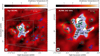 |
Fig. 1 Partly taken from Möller et al. (2023). Continuum emission toward Sgr B2(M) at 242 GHz. A close-up of the central part is presented in the right panel. The identified sources are marked with shaded blue polygons and indicated with the corresponding source ID. The shaded light blue polygons describe the inner cores. The black points indicate the position of each core, described by Sánchez-Monge et al. (2017). The intensity color scale is shown in units of brightness temperature, and the synthesized beam of 0″.4 is described in the lower left corner. The green ellipses describe the H II regions identified by De Pree et al. (2015), where the size of each ellipse indicates to the size of the corresponding H II region. |
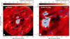 |
Fig. 2 Partly taken from Möller et al. (2023). Continuum emission toward Sgr B2(N) at 242 GHz. The right panel describes a close-up of the central part. The shaded blue polygons together with the corresponding source ID indicate the identified hot cores. The shaded light blue polygons describe the inner cores. The black points indicate the position of each core described by Sánchez-Monge et al. (2017). The intensity color scale is shown in units of brightness temperature, while the synthesized beam of 0″.4 is indicated in the lower left corner. The green ellipses describe the H II regions identified by De Pree et al. (2015), where the size of each ellipse indicates to the size of the corresponding H II region. |
4 Results
In this section, we describe the molecules and their isotopologs and vibrational excited states identified in the line surveys of each source in Sgr B2(M) and N. Due to their chemical relationships, for example having the same heavy-atom backbone or the same functional group, the detected molecules are divided into eight families: Simple O-bearing molecules (Appendix E.1 (page 15)), complex O-bearing molecules (Appendix E.2 (page 18)), NH-bearing molecules (Appendix E.3 (page 19)), N- and O-bearing molecules (Appendix E.4 (page 19)), cyanide molecules (Appendix E.5 (page 20)), S-bearing molecules (Appendix E.6 (page 22)), carbon and hydrocarbons (Appendix E.7 (page 24)), and other molecules (Appendix E.8 (page 24)).
Cold gas in the interstellar medium is often made up of simple molecules (e.g., CO, HCN, N2, O2 etc), which are frozen onto dust grains. Both hydrogenation and reactions with CO produce more complex molecules on the dust surface; for example, CO2, CH3 OH, and H2O. UV radiation can cause some of these molecules to dissociate into radicals. With increasing temperature, these radicals become mobile and form new species. When the temperature is high enough (T ~ 100–150 K), the ice mantles sublimate and the resulting molecules enter the gas phase and form, among other things, precursors of complex organic molecules (COMs) (Taquet et al. 2016). In addition, shocks generated by the interaction of jets and outflows with the surrounding envelope can also sublimate or sputter icy grain mantles, releasing molecules such as CH3OH and other COMs into the gas-phase. Furthermore, shocks can also sputter the grain cores themselves, releasing the embedded Si and S atoms and increasing the production of Si- and S-bearing species such as SiO, SO2 and SO (see e.g., Gusdorf et al. 2008; van Dishoeck 2018). It is important to note that while grain-surface chemistry plays a significant role in the formation of COMs, these molecules can also form in the gas phase. Various models, such as those by Vasyunin et al. (2009) and Wang et al. (2021), suggest that gas-phase reactions contribute significantly to the synthesis of COMs.
The derived excitation temperatures and abundances for each detected molecule and source in Sgr B2(M) and N, respectively, are shown in Appendix G (page 109) and H (page 113). For molecules for which more than one component was required, we give the column density weighted mean temperature and the summed abundances. We calculated the abundances relative to H2 using the hydrogen column densities derived in our first paper for each source. A comparison between the obtained temperature and abundance ranges for each source in Sgr B2(M) and N and literature values are given in Table E.1 (page 16)–E.2 (page 17), respectively. In general, a direct comparison of the obtained temperatures and abundances with previous analysis is of limited value. First, compared to Sutton et al. (1991); Belloche et al. (2013); Neill et al. (2014), and Möller et al. (2021), our observations have a much higher spatial resolution, which is why we can detect structures that could not be included in these analyses.
Only the observations of Bonfand et al. (2017) have a similar resolution. Nevertheless, our analysis differs significantly from previous analyses in some aspects, because we determined not only the dust and free-free contributions to each source but in addition considered effects such as local overlap effects, which are important for line-rich sources such as Sgr B2(M) and N.
A detailed description of all identified species together with figures showing the spectra of each detected molecule is provided in Appendix E (page 15)–F (page 25). For molecules with a large number of transitions, a representative selection of the detected transitions is shown8.
Velocity ranges
5 Discussion
5.1 Physical parameters
To better understand the distribution of the derived physical parameters, we computed in addition to the mean temperatures of each source and layer shown in Figs. G.1 (page 109)–G.4 (page 112), kernel density estimations (KDE, Rosenblatt 1956; Parzen 1962) with a Gaussian kernel for each source, layer and molecular family, see Figs. I.1 (page 118)–I.12 (page 129). Here, we consider only those components that clearly belong to Sgr B2; that is, whose source velocity is greater than 22 km s−1 (see Table 1). In addition, we take only those molecules into account, which show more than one transition within the frequency ranges covered by our observations. Furthermore, Silverman’s rule (Silverman 1986) as scipy implementation (Virtanen et al. 2020) is used to compute the bandwidth of each KDE. For a better visibility, we have normalized the maximum of each KDE to one. In general, the KDE is a nonparametric way to estimate the probability density function of a given parameter and offers a visual representation of the individual parameters with the aim to see their spread and to search for general trends. The shape of the KDE plot can provide insights into the underlying distribution of the data. For example, a unimodal KDE plot with a single peak suggests that the data is distributed around a central value, while a bimodal KDE plot with two peaks suggests that the data may be drawn from two different distributions.
The KDEs of excitation temperatures of components belonging to the envelope layer in both regions mostly show an unimodal distribution with maxima located at around 20 K for most sources and molecular families, see Figs. I.1 (page 118) and I.3 (page 120). This is remarkable because in our analysis of continuum contributions (see Möller et al. 2023) we found excitation temperatures in the envelopes of around 73 K (for sources in Sgr B2(M)) and 59 K (for sources in Sgr B2(N)). A possible explanation for this may lie in the way the excitation temperatures were determined in Möller et al. (2023), where we selected pixels around each source and used the spectra at these positions to compute an averaged envelope spectrum. Afterward, we analyzed the contributions of CH3 CN, H2CCO, H2CO, H2CS, HNCO, and SO to these envelope spectra to determine the averaged gas temperature in each envelope. Details of the calculation procedure are described in Möller et al. (2023). In contrast to the molecules in the current analysis located in the envelope layer, these molecules are seen more or less in emission only. But emission features from the envelope toward the sources cannot be separated from the core. Molecules in emission have mostly higher temperatures than molecules in absorption. Therefore, we underestimate in this analysis the real excitation temperatures in the envelopes around each source.
For the inner sources in Sgr B2(M) and N – those located less than 50 au from the center of the central core A01 for both regions – we find broader distributions of simple O-bearing and cyanide molecules, while the NH-bearing molecules are usually at lower temperatures. A possible explanation for this behavior could be the high contributions of H2CO, CH3OH, HCN, and HNC in the inner sources, which are hot and very close to each other heating up the surrounding envelope. For sources A08, A09, A20, and A22 in Sgr B2(M), the maximum of the KDE of sulfur-bearing molecules is shifted toward slightly higher temperatures. The formation and abundance of certain sulphur-bearing molecules, such as SO and SO2, are positively correlated with the kinetic temperature (Fontani et al. 2023), suggesting that these molecules become more abundant as the temperature increases through the evolutionary stages. Therefore these molecules are usually located in the warmer regions of the envelopes. For some inner sources in Sgr B2(N), we find slightly broader distributions of simple O-bearing and NH-bearing molecules. Additionally, for source A07 the different molecular families show clear separated maxima, where the sulfur-bearing molecules, as in source A14, are the hottest.
The KDEs of temperatures whose components are located in the core layer of Sgr B2(M) show a very different behavior, see Fig. I.2 (page 119). While the inner sources show broad distributions for many molecular families, we see narrower and sometimes spike-like9 KDEs in the outer sources. This is due to the fact that many outer sources are mainly seen in absorption and have fewer emission features. In many sources, the sulfurbearing molecules exhibit the highest temperatures, which, in addition to the fact that these molecules require high temperatures for formation, can also be explained by the fact that molecules of this family often exhibit vibrationally excited states with high excitation temperatures. For sources in Sgr B2(N) the temperatures in the core layer show, in contrast to sources in M, much narrower distributions, see Fig. I.4 (page 121). The sources in N thus seem to have a more homogeneous structure.
For the line widths, we obtain KDEs with mostly unimodal distributions in all sources, layers, and molecular families, see Figs. I.5 (page 122)–I.8 (page 125). However, the distribution between the different families of molecules and sources is sometimes very different. As for the excitation temperatures, in both regions the outer sources show narrower distributions than the inner sources. In general, the line width contains among other things a thermal and a turbulent proportion, where the thermal one depends on the gas temperature and the respective molecular weight. For all molecular families and sources the thermal line widths range from 0.1 to 0.6 km s−1. Therefore, the distribution of line widths mainly shows the turbulent contribution. Line widths above 10 km s−1 indicate outflows or large-scale motions. Some sources show significant differences between molecular families. For example, in source A20 in Sgr B2(M), the N- and O-bearing molecules in the core layer show a significantly larger line width, see Fig. I.6 (page 123), and a larger velocity offset, see Fig. I.10 (page 127), than the other molecules, which could indicate that it cannot be directly assigned to the hot core A20 but to a filament. In addition, some molecules show high asymmetric line shapes, which can be associated with outflows. The description of these line shapes requires many components, which falsifies the true distribution of line widths.
By using the distributions of velocity offsets, it is possible not only to determine the velocity of each source, but also whether certain families of molecules show deviations from it, which in turn can indicate a different affiliation. A deviating source velocity could, for example, show that the associated molecular family does not belong to the source in question, but to a filament located in front of the source. For example, the distributions of velocity offsets of the different molecular families in the core layer of source A14 in Sgr B2(M) show clear differences. While the N- and O-bearing and sulfur-bearing molecules show more or less the same velocity offsets, we see clear shifts toward higher velocities for simple O-bearing, cyanide, and NH- bearing molecules. A similar but less pronounced behavior can be found among others for source A08, A15, and A22. In general, we find, in both regions, broader distributions in the envelope than in the core layer for most sources.
5.2 Correlations between sources
To find correlations between different sources in Sgr B2(M) and N that might indicate similar evolutionary phases, we used the principal component analysis (PCA). PCA is a widely used multivariate analysis method that uses an orthogonal transformation to convert observed variables into a set of linearly uncorrelated new variables called principal components. The first principal component contains the largest possible variance, and the subsequent principal component has the next highest variance, provided that it is orthogonal to the previous component. In contrast to other PCA analyses (e.g., Gratier et al. 2017; Kim et al. 2023), we do not apply PCA directly to the observed spectra, but use the calculated abundances relative to the hydrogen column densities derived in our first paper for each source of the core components10 for the different sources (see Figs. H.2 (page 114) and H.4 (page 116)) whose source velocity is greater than 22 km s−1 . By using abundances, the results of the PCA are not distorted by line overlap or absorption features. Furthermore, we do not need to normalize the spectra, nor do the spectra of the different sources need to be corrected due to the different source velocities. Here, we assume that two sources of the same age also have great similarities in the sequence of their abundances. However, the abundances can be distorted by contributions from filaments, foreground objects and imaging artifacts. Furthermore, many spectra from sources located further out in Sgr B2(M) and N have a significantly lower signal-to-noise ratio than the inner sources, which makes the identification of molecules and the determination of the physical parameters more difficult. This in turn can lead to incorrect PCA results, whereby correlations that are not real are identified. For our analysis, we have used the PCA implementation available in the Python package scikit-learn (Pedregosa et al. 2011).
The percentages of eigenvalues are shown in Fig. 3. For both regions, the first eigenvalue has the highest proportion (49.7% for Sgr B2(M) and 34.2% for Sgr B2(N)), while the first six principal components together account for more than 80% of the total variance for both regions.
The first six eigenvectors for each region are described in Figs. D.3 (page 9)–D.4 (page 10). For sources in Sgr B2(M), the first eigenvector is mainly dominated by contributions from outer sources, in particular by A20, while the remaining eigenvectors exhibit relatively uniform distributions. Similarly, for Sgr B2(N), the first eigenvector again shows the most significant contributions, with the outer sources A09, A12, and A13 being dominant, while the other eigenvectors display a more consistent structure.
The abundances of each source in Sgr B2(M) and N can now be projected onto a pair of principal components (see Figs. D.1 (page 7)–D.2 (page 8)). After transforming the data into the principal component space, the k-means (Hartigan & Wong 1979) function from the scikit-learn package is used to categorize the cores into a predefined number of distinct, non-overlapping clusters. In order to obtain the best number of clusters, we apply the elbow method (Thorndike 1953) using the yellowbrick Python package (Bengfort & Bilbro 2019), which involves plotting the within-cluster sum of squares (WCSS) against the number of clusters (see Fig. 4). The point of maximum curvature in the plot called elbow or knee represents the point where the WCSS starts to decrease at a slower rate. This point indicates the appropriate number of clusters. For sources in Sgr B2(M), the elbow is at six and for N at seven clusters. The identified cluster together with the contained sources for both regions are shown in Table 2.
The projection of the first two eigenvectors PC1 and PC2, which together have a variance of more than 57% for both regions, shows a clear separation between different sources in Sgr B2(M). For each identified cluster and region in this projection of PC1 and PC2, we calculated the mean abundances (see Fig. D.5 (page 11) (for Sgr B2(M)) and Fig. D.6 (page 12) (for Sgr B2(N)), and the mean temperatures, see Fig. D.7 (page 13) (for Sgr B2(M)) and Fig. D.8 (page 14) (for Sgr B2(N))) for each identified molecule. In addition to the level of evolution of the source, other contributions such as filaments can also play a role in the classification of the sources into the various clusters.
The temperature and abundances dispersions for each cluster in Sgr B2(M) are described in Fig. 5, which show more a less a unimodal behavior. Clusters CM1 and CM4 in Sgr B2(M) have similar abundances for most molecules, with t-HCOOH and NH2CN found exclusively in cluster CM1, and c-C3H2 only in cluster CM4. Furthermore, cluster CM1, which contains most of the inner sources, has the highest mean temperatures of all species and clusters. In addition, the cluster has the highest mean temperature for the sulfur-bearing molecules except NS. This could indicate that the sources contained in these two clusters are in later stages of evolution, where more complex molecules such as C2H5OH can also form. Furthermore, the presence of vibrationally excited molecules, such as C2H3CN,v10=1 (Elow = 1662.9 K) and C2H5CN,v20=1 (Elow = 694.0 K), indicates that the protostars have already reached high temperatures, which in turn suggests an advanced state of evolution. As cluster CM1 shows slightly higher mean temperatures than cluster CM4, the majority of sources in this cluster appear to have progressed furthest in their development. In contrast to that, sources in cluster CM2 exhibits the lowest mean abundances of CH3OH, H2CCO, CH3 CN, C2H5CN, HCCCN, OCS, and its vibrational state OCS,v2=1 and the highest abundance of CCH. Furthermore, this cluster also shows the lowest mean temperature of methanol. Both together suggest that the sources in this cluster are in earlier stages of evolution. In addition, cluster CM3 has the lowest mean abundances for SO, H2 CCN, H2CS, HNCO, NH2D, CH3OCH3 , and H2CO, while OCS, OCS,v2=1, H2CS, and HCCCN show the lowest mean temperatures, again indicating a fairly early stage of development. Cluster CM5 containing only source A20 has the lowest abundances of SO2 and its vibrational state SO2,v2=1, NO, and CH3OCHO. At the same time, this source shows the lowest mean temperatures for SO, NO, and CH3OCHO, which again suggests an early phase of evolution. Finally, cluster CM6 has the lowest mean abundances for SiO, CH2 NH, CN, and NS of all clusters. In addition, this cluster exhibits the highest mean temperatures for NO on the one hand and the lowest mean temperatures for NS, H234S, HCS+, SO2, SO2,v2=1, HC(O)NH2, HNCO and H2CO on the other, which makes it difficult to classify the cluster into an evolutionary stage.
For Sgr B2(N), we find a somewhat larger number of clusters, two of which consist of only two elements and one of which consists of only one element. The temperature and abundances dispersions for each cluster in Sgr B2(N) are described in Fig. 6. Cluster CN1 exhibits the lowest mean abundances of CH3 OH, H2CCO, CH3OCHO, and CN, as well as the lowest mean temperatures for CH3OH, H2CCO, and SiO. This could indicate that the sources in this cluster are in early stages of evolution. The cluster CN2 shows the lowest mean abundances for C2H5OH, CH3CHO, CH3NH2, HC(O)NH2, C2H3CN, C2H3CN,v10=1, C2H5CN, C2H5CN,v20=1, HCCCN,v7=2, SO2, and SO2,V2=1. Furthermore, the lowest temperatures are also found in this cluster for many of these molecules; that is, CH3OCH3, C2H5OH, CH3OCHO, CH3CHO, CH2NH, HC(O)NH2, C2H3CN, C2H5CN, H234S, SO2, SO2,v2=1, and OCS,V2=1. At the same time, this cluster contains the highest abundances for NO and SO and the highest mean temperatures for NO, C2H3CN,v10=1, and HCCCN,v7=2. In addition, cluster CN2 is the only cluster that contains NH2D. This behavior indicates a very heterogeneous source structure, so that no statement can be made about the state of development. For cluster CN3, we found the highest mean abundances for several molecules – H2CO, SiO, CH3OCH3, CH2NH, C2H3CN, C2H3CN,V10=1, C2H5CN, C2H5CN,v20=1, HCCCN, v7=2, H234S, SO2, and NS – and the highest mean temperatures for CH3OH, H2CCO, SiO, C2H5OH, CH3CHO, CH2NH, HNCO, C2H3CN, C2H5CN, C2H5CN,V20=1, SO, SO2,v2=1, OCS, and OCS,v2=1. The lowest temperature of H2CO, CH3NH2, and CH3NH2 is also found in this cluster. In summary, the high temperatures and the high abundances of some vibrationally excited states indicate that the majority of the sources in this cluster are at higher evolutionary stages. Cluster CN4 exhibits the highest mean abundances of CH3OH, H2CCO, C2H5OH, CH3OCHO, CH3CHO, CH3NH2, HNCO, HC(O)NH2, HCCCN, H2CS, and OCS,v2=1, as well as the highest mean temperatures for H2CO, CH3OCHO, CH3NH2, HC(O)NH2, HCCCN, H234S, SO2, and H2CS. In contrast, NS has the lowest concentration, and C2H3CN,v10=1, C2HsCN,V20=1, HCCCN,V7 =2, and NS have the lowest mean temperatures. This could indicate that the sources in this cluster are in an intermediate stage of development, at which the temperature is still too low to excite vibrationally excited states sufficiently. The cluster CN5, which contains only source A13, shows the lowest mean abundances for CH3OCH3, CH2NH, H234S, and OCS on the one hand and the highest mean temperatures for CH3OCH3 and NS on the other. In addition, we find that HCCCN has by far the lowest excitation temperature of all clusters. This unusual behavior could indicate a more complex source structure. In the case of cluster CN6, the mean abundance is lowest for H2CO, HNCO, SO, and OCS,v2=1, and highest for CH3CN, CN, and CCH. Additionally, the lowest mean temperatures are found for CH3CN, H2CS, and CCH, while the highest temperature is found for CN within this cluster. As with the previous cluster CN5, this behavior indicates again a more complex source structure. Finally, cluster CN7, shows the lowest mean abundances for SiO, NO, CH3CN, HCCCN, and H2CS, and the lowest mean temperatures for NO and OCS. However, this cluster also shows the highest temperature for CH3CN, which may be due to inaccuracies in the fit. The sources contained in this cluster have been found to contain only a small number of molecules, which also show relatively low mean temperatures. This indicates that the sources in this cluster are still in a relatively young phase of evolution.
The Kendall correlation coefficient (Kendall 1938) analysis offers another possibility to find correlations between different sources in a more rigorous and unbiased way. The coefficient, commonly referred to as Kendall’s τ coefficient11, is applied to the calculated abundances of the core components for the different sources for both regions, whose source velocities are greater than 22 km s−1. The coefficient is calculated for each pair of sources and is given by
 (2)
(2)
where n represents the number of paired observations and xi, xj are the observations of the first and yt, yj are the observations of the second variable, respectively. The coefficient is used to measure the ordinal association between two measured quantities. It is particularly suitable for ordinal variables and is a nonpara-metric measure of the strength and direction of association that exists between two variables. The coefficient ranges from −1 to 1, where 1 indicates perfect agreement, −1 indicates perfect disagreement, and 0 indicates no association. Setting an (arbitrary) threshold at >|0.9| to indicate a good correlation (see Figs. J.1 (page 130)–J.2 (page 131)). For sources in Sgr B2(M) we find strong correlations between A08 and A14 (both are located in cluster CM4 and are next to each other), A18 and A19, A18 and A21, A19 and A21, and between A21 and A24 (all contained in cluster CM6). Source A20, on the other hand, shows a remarkably low correlation (≤ |0.5|) with most of the other sources. There appears to be a somewhat greater correlation only with sources A16, A17, A22 and A25, although these sources are not located in the vicinity of A20. The correlations for sources in Sgr B2(N) are generally smaller than in Sgr B2(M). Strong correlations are found between sources A09 and A14, and between A09 and A15 (all sources are located in cluster CN6) and between A11 and A12 (both part of cluster CN7). In addition, there are also strong correlations between sources A09 and A11 and between A11 and A16 although the respective sources are not in the same cluster. For example, source A09 belongs to cluster CN6 and source A11 to cluster CN7. The correlation between sources A11 and A16 is remarkable, as neither source is neighboring and A16, in contrast to source A11, contains an H II region, which is why both sources are in different evolutionary stages. There is also a particularly low correlation between sources A13 and A17.
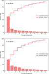 |
Fig. 3 The percentages of the first eleven eigenvalues in descending order for sources in (a) Sgr B2(M) and (b) Sgr B2(N). |
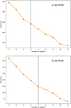 |
Fig. 4 Elbow plot for sources in (a) Sgr B2(M) and (b) Sgr B2(N). |
Clusters identified by the k-means algorithm.
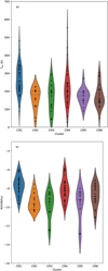 |
Fig. 5 Violin plots describing (a) temperature and (b) abundance distributions for each cluster in Sgr B2(M). Here, the long dashed lines describe the respective medians, while the short dashed lines represent the quartiles of the data, which are also described as black dots. |
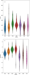 |
Fig. 6 Violin plots show (a) temperature and (b) abundance distributions for clusters in Sgr B2(N). Long dashes represent medians, short dashes mark quartiles, and black dots depict data points. |
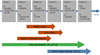 |
Fig. 7 Evolutionary sequence as proposed by Bonfand et al. (2017) for the hot cores embedded in the Sgr B2 complex based on Fig. 5 of Codella et al. (2004), along with the “straw man” model (Ellingsen et al. 2007) that shows the lifetimes of various maser species. |
5.3 Evolutionary sequence in Sgr B2(M) and N
Following Codella et al. (2004) and Bonfand et al. (2017), we used the distributions of masers, outflows and H II regions to determine the evolutionary sequence and age of the different hot cores in the Sgr B2 complex (see Fig. 7).
Codella et al. (2004) proposed an evolutionary scheme for high-mass star forming regions, where class II methanol masers are formed before H II regions can be observed, because the masers are thought to be associated with deeply embedded, high-mass protostars that are not evolved enough to ionize the surrounding gas and produce a detectable H II region. In the next phase, maser and H II region coexist, where the methanol molecules are shielded from the central UV radiation by the warm dust in the slowly expanding molecular envelope of the UCH II region, whose emission also provides its pumping photons. After 2.5 × 10⁴ to 4.5 × 10⁴ yr (depending on the assumed initial mass function (IMF), van der Walt 2005), the maser emission stops as the UCH II region continues to expand. However, this analysis is complicated by the fact that we have averaged the spectra of each source over several pixels in order to obtain a better signal-to-noise ratio. This means that the averaged spectra may contain contributions from different protostars. For example, the polygon of core A01 in Sgr B2(M) contains six H II regions and more than 33 masers (see Table 3), indicating that core A01 includes multiple protostars.
5.3.1 Maser
As is described by Fig. 8 many sources in Sgr B2(M) and N contain a variety of masers. Methanol masers are commonly found in the early stages of high-mass star formation and are associated with the presence of hot molecular cores (Fontani et al. 2010; Yang et al. 2023). They are known to trace the processes of mass accretion and outflow in these region. They are classified into two series of transitions called class I and class II. Class I methanol masers are excited by collisional processes, such that they are often found in outflows and interacting regions between outflows and dense ambient gases, usually offset from the associated protostellar object (Matsumoto et al. 2014). The 70 – 61A+ methanol maser at 44 GHz is representative of the class I methanol maser and was found only in the envelope of Sgr B2(N), see Fig. 8. Class II methanol masers are radiatively excited and closely associated with high–mass proto– stars, because the pumping requires dust temperatures >150 K, high methanol column densities (>2 × 1015 cm−2), and moderate hydrogen densities (nH < 108 cm−3). The 51 – 60A+ class II methanol transition at 6.7 GHz in particular is the strongest and most widespread of the methanol masers (Sobolev et al. 1997). The sources12 A04/A05 in Sgr B2(M) as well as A08 and A13 in Sgr B2(N) contain a single class II methanol maser, respectively. Moreover, H2O masers, are primarily located in the inner sources of Sgr B2(M) (A01, A02, A06, A07, A08, A10, A11, and A21) and N (A01, A02, A03, A04, A07, and A08). Similar to methanol masers, water masers tend to disappear as an UCH II region develops. These masers are also directly connected to molecular outflows (Codella et al. 2004). Furthermore, they are often associated with shocks resulting from the interaction of dense molecular outflows with the surrounding medium (Elitzur et al. 1989). The characteristics of H2O masers can help to understand the distribution of water vapor and the impact of shocks and radiation on its abundance (van Dishoeck et al. 2021). Moreover, ammonia (NH3) masers are also found in the early stages of high-mass star formation and are associated with the presence of dense, hot molecular cores (Mei et al. 2020; Yan et al. 2022b). They are known to trace the presence of high-density gas and strong shocks and are often used to study the processes of mass accretion and outflow. Similar to H2O masers, NH3 masers are predominantly found in the inner sources of Sgr B2(M) (A01, A02, A03, A05, and A07) and N (A01, A02, and A08). Additionally, formaldehyde (H2CO) masers are relatively rare and have been observed in a few high-mass star-forming regions. They are known to indicate the presence of high-velocity shocks and are found in many sources, especially in the inner parts of Sgr B2(M) (A01, and A02) and N (A02, A03, and A08), respectively. Finally, OH masers are typically associated with the late stages of high-mass star formation and are often found in regions with evolved stars or supernova remnants (Wu et al. 2006). Additionally, OH masers are known to detect the presence of high-speed shocks and are often used to study the magnetic fields in these regions, among other things. The sources in Sgr B2(M) in particular contain a large number of OH masers (A01, A02, A03, A06, A10, A16, and A26), whereas only source A04 in Sgr B2(N) contains such a maser.
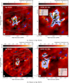 |
Fig. 8 Sources in Sgr B2(M) and N together with the positions of the different masers. A close-up of the central part is presented in the right panel. The identified sources are marked with shaded blue polygons and indicated with the corresponding source ID. Similar to Figs. 1–2, the shaded light blue polygons describe the inner cores of the corresponding region. The black points indicate the positions of each source described by Sánchez-Monge et al. (2017). The intensity color scale is shown in units of brightness temperature and the synthesized beam of 0″.4 is described in the lower left corner. The green ellipses describe the H II regions identified by De Pree et al. (2015). The markers indicate the positions of published maser detections from the 44 GHz class I (Mehringer & Menten 1997) and from the 6.7 GHz class II methanol masers (Caswell 1996; Hu et al. 2016; Lu et al. 2019). Additionally, the positions from H2CO (Whiteoak et al. 1987; Mehringer et al. 1994; Lu et al. 2017), H2O (McGrath et al. 2004), NH3 (Martín-Pintado et al. 1999; Mills et al. 2018; Yan et al. 2022a), OH (Gaume & Claussen 1990; Yusef-Zadeh et al. 2016), and SiO (Morita et al. 1992; Shiki & Deguchi 1997; Zapata et al. 2009) masers are described as well. The red crosses and names indicate the hot cores in Sgr B2(N) identified by Bonfand et al. (2017). |
Evolutionary phases of the individual sources in Sgr B2(M) and N.
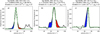 |
Fig. 9 Example of transitions used to identify outflows toward Sgr B2(M) and N. The vertical dashed line marks the systemic velocity of the Sgr B2 complex and the high velocity wings are indicated in blue and red. The black line describes the observational data, while the green line represents a fit with a single Gaussian to emphasize the non-Gaussian wings of each peak. (a) Some transitions show more or less symmetric, non-Gaussian line shapes. (b) In addition, some transitions contain contributions from an isotopolog or another molecule. (c) There are also some transitions that show a strongly asymmetric line shape. |
5.3.2 Outflows
The evolutionary sequence, as is shown in Fig. 7, requires the identification of outflows. In general, the study of outflows in high-mass star-forming regions can provide crucial information about the formation and evolution of massive stars. The momentum injected by outflows may limit accretion onto the massive star, potentially setting an upper mass limit to the stellar initial mass function. Additionally, there is a decrease in jet activity with evolutionary time in high-mass star-forming regions (Arce et al. 2007).
The line profiles of the outflow tracers (e.g., SiO, SO, and OCS) show high velocity emissions and non-Gaussian linewings that are likely associated with out flowing gas at blue- and red-shifted velocities compared to the systemic velocity of the source (see Fig. 9). In addition to outflows, rotation and infall motions can also lead to red and blue asymmetric line profiles, where infall usually produces stronger blue- than red- shifted emission (Fuller et al. 2005). Here, we assume that all non-Gaussian line-wings indicate outflows. (Due to its large optical depth, SiO shows self-absorbing line profiles, which is why we do not consider it further in the analysis.)
Sulfur monoxide (SO) and carbonyl sulfide (OCS) are excellent outflow tracers due to their strong, high-velocity line wings, and spatial distributions. In high-mass star-forming regions, SO and OCS have several advantages as outflow tracers. Unlike other molecules, SO and OCS are less confused by emission and absorption by unrelated molecular clouds, making these valuable tracers of outflow activity in these regions (Hatchell et al. 2001).
When analyzing the outflow components, it is important to consider that the line shape may contain other contributions. For instance, a filament in front of the source, which also contains an outflow tracer such as SO, can impact the line shape. Depending on the temperature of this gas, it can result in a lateral peak or an additional absorption structure in the line shape, as illustrated in panel b and panel c in Fig. 9, respectively. The detection of outflows in the inner sources in Sgr B2(N) is complicated by strong overlap of other molecular lines. In order to be able to estimate these contributions, the gas would have to be examined in detail not only in the hot cores but also between the cores in order to precisely determine the expansions of the filaments and the outflows.
5.3.3 Classification according to evolutionary phase
The classification of each sources in Sgr B2(M) and N into the individual evolutionary phases described in Sect. 5.3, is shown in Table 3. For sources A14 in Sgr B2(M) and A05 and A17 in Sgr B2(N) we found evidences of outflows, but neither masers nor H II regions. Perhaps the associated H II regions are too small, which is why they have not yet been discovered. However, the asymmetrical line profiles could also have other causes, such as infall motions. Sources A15 and A24 in Sgr B2(M), which roughly correspond in position and size to a single H II region, and sources A10 and A16 in Sgr B2(N) show the highest evolutionary phase. In general, the inner sources in the two regions Sgr B2(M) and N, which are located within a distance of less than 50 au around the central core A01, are usually in a more advanced phase than the outer sources (see Fig. 10).
Exceptions are the sources A24 and A26 in Sgr B2(M) and A16 in Sgr B2(N). We have identified the same evolutionary stages for sources A08 (associated with N3) and A13 (associated with N4) in Sgr B2(N) as are reported by Bonfand et al. (2017). However, we assign the inner source A01 (N1) to an earlier evolutionary stage due to the presence of H2O masers. According to our analysis, source A02 (N2) is at a significantly later evolutionary stage as classified by Bonfand et al. (2017), as we not only consider the occurrence of H2O maser, but also identify outflows in this source. This difference may be attributed to the fact that Bonfand’s source N2 in our analysis comprises two sources (A02 and A03).
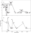 |
Fig. 10 Evolutionary phases as function of the distance from the center from the respective region for (a) Sgr B2(M) and (b) Sgr B2(N). |
5.4 Chemical clocks
In addition to the methods described above, the abundances of certain molecules can be used to determine the age of a source. Chemical tracers that show empirical relations between their abundances and the different phases of the star formation process are often referred to as chemical clocks (see e.g., Charnley 1997; Hatchell et al. 1998). Some molecules become abundant (or disappear) after a certain evolutionary phase, while other tracers may show a constant increase (or decrease) throughout the evolutionary sequence. Chemical clocks are based on the relative abundances ratios of different molecular species. In the following we use the abundances derived in Sect. 4 for the core components13 (see Figs. H.2 (page 114) and H.4 (page 116)), to estimate the evolutionary sequence of each source in Sgr B2(M) and N.
Charnley (1997); Hatchell et al. (1998) and Herpin et al. (2009) propose the usage of the relative abundance ratios of OCS, SO, SO2 and H2S as chemical clocks, because the main reservoir of sulfur on grain mantles is H2S. (Recent observations by McClure et al. (2023) using the James Webb Space Telescope (JWST) have provided new insights into the composition of ices in dense molecular clouds. Contrary to previous assumptions, H2S was not detected as a major component in these ices. Shingledecker et al. (2020) identified cyclic octatomic sulfur (S8) as a potential alternative reservoir of sulfur on grain surfaces. However, for the purposes of the further analysis, we shall maintain the assumption that H2S remains the primary reservoir for sulfur on dust mantles. This approach allows coherence with existing models while taking into account the need for future refinements based on these new observations.) When the dust temperature in the hot core exceeds the mantle evaporation temperature, all components of the grain mantles, including hydrogen sulfide, are suddenly injected into the gas phase (Wakelam et al. 2004a). Subsequently, endothermic reactions in the hot gas transform H2S into atomic sulfur and SO, leading to the formation of more SO and afterward to SO2 on timescales of ~103 yr. Therefore, the SO2/SO and SO/H2S ratios are functions of time and can thus indicate the age of the hot cores (Wakelam et al. 2004a). In addition, Wakelam et al. (2011) predict an increase in the SO2/OCS and SO2/H2S ratios for sources with more evolved chemistry. Since H2S has no transition in the frequency ranges covered by our observations, we only use the ratios of SO2/OCS and SO2/SO to estimate the age.
In addition to sulfur-bearing molecules, complex cyanides, especially those containing the CN group, have also been identified as possible chemical clocks in high-mass star-forming regions. Belloche et al. (2009) and Garrod et al. (2017) suggested that the formation of C2H5CN on grains occurs through the hydrogenation of C2H3CN, which is formed from HCCCN during the collapse and warm-up phase. Subsequently, C2H5CN sublimates to the gas phase at a temperature of 100 K (Garrod et al. 2017). The majority of the C2H5CN formed on the grains is subsequently eliminated by gas-phase reactions. In their chemical simulations, Belloche et al. (2014) observed a reduction in the gas phase abundance of C2H5CN and an increase in the abundance of C2H3CN after approximately ~3.5 × 10⁵ yr. Here, we use the ratio of ethyl cyanide to vinyl cyanide as a chemical clock, similar to Bonfand et al. (2017). According to Minh et al. (2016), the formation of CH3CN is anticipated to occur at a later stage than CH3OH. Therefore, comparing the abundances of these two species can serve as a reliable indicator of the evolutionary timescale during the initial phases of massive star formation. The CH3CN/CH3OH abundance ratios are expected to be low during the very early phase of grain mantle evaporation and increases over time by the production of CH3CN and the destruction of CH3OH through its transformation into other complex species. As was discussed by Rodgers & Charnley (2001), CH3OH maintains a high abundance until the age of around 104 yr, after which it begins to be depleted. Over the next 105 yr, the abundance of CH3CN is expected to increase, reaching a level only a few times less than that of CH3OH. However, Garrod et al. (2022) have revealed a more nuanced understanding of cyanide formation and abundance in these environments. While the formation of C2H5CN on grains through hydrogenation of C2H3CN remains a viable pathway, the gas-phase chemistry of cyanides at high temperatures has been shown to play a significant role. The revised models indicate that certain N-bearing molecules, especially cyanides, experience substantial enhancement through gas-phase chemistry at temperatures above 100 K. HCN and CH3CN, in particular, see their greatest gas-phase production at very high temperatures exceeding 300 K, with considerable production also occurring between 120–160 K as ice-mantle material sublimates. This new understanding complicates the use of cyanide abundance ratios as simple chemical clocks. The CH3CN/CH3OH abundance ratio, previously thought to increase steadily over time due to CH3CN production and CH3OH destruction, may now be influenced by high-temperature gas-phase chemistry. This additional production pathway for CH3CN could potentially accelerate its abundance increase relative to CH3OH, altering the expected temporal evolution of their ratio.
However, it is important to note that the ratios are also influenced by physical conditions and the composition of grain mantles, making their interpretation as standalone indicators of age challenging (Vidal & Wakelam 2018). Determining the exact age of each source would require complex chemical modeling of each individual source, which would go beyond the scope of this paper. Furthermore, we cannot completely exclude the possibility that one or the other emission belongs to a filament rather than a hot core, which would falsify the determination of the abundances as well. It should also be noted that the sources identified by Sánchez-Monge et al. (2017) sometimes consist of several individual hot cores.
The evolutionary sequences obtained from the different chemical clocks are described in Table 4, where the sources in each row are ordered from young to old (evolved). In addition to the abundance ratios described above, we also consider the abundance ratios of vibrationally excited molecules, as these species describe the innermost, hottest part of each source. The orders of the sources based on the ratios of vibrationally excited molecules are broadly consistent with the orders determined using the abundance ratios of non-vibrationally excited molecules. In general, we do not obtain a uniform order of the various sources in Sgr B2(M) and N. In the following discussion, the evolution phase of a source, as is described in Table 3, is indicated in round brackets.
For sources in Sgr B2(M), sulfur-bearing molecule ratios suggest A20 (evolution phase I) and A26 (IV) as young sources, A03 (III), A13 (I) and A12 (I) as intermediate, and A14 (no classification) and A08 (IV) as evolved. These results largely align with previous analyses, with A26 being a notable exception, possibly due to its complex substructure. The H II region, which is decisive for the classification of the source A26 into phase IV, only covers a small part of the source, so that it can be assumed that the source is not monolithic, but has a complex substructure consisting of several sources. Cyanide-based ratios, however, present a different picture, classifying A0 (IV), A01 (IV), and A10 (III) as young, A05 (II) and A07 (IV) as intermediate, and A03 (III), A04 (IV), and A06 (III) as evolved. These discrepancies may be attributed to the potentially complex substructures within these sources, many of which contain multiple H II regions and/or maser emissions.
In Sgr B2(N), our analysis using sulfur-bearing molecules indicates A08 (III) and A06 (I) as young sources, A04 (III) as intermediate, and A10 (V) as evolved, generally corroborating previous analyses except for A08. Conversely, cyanide-based ratios suggest A01 (IV) as young, A06 (I), A04 (III), and A02 (III) as intermediate, and A08 (III) as evolved. The disparities in classifications, particularly for A01 (IV) and A08 (III), may be attributed to their complex substructures.
Our study highlights the challenges in determining the evolutionary stages of sources within the Sgr B2 complex. The results of our analyses for each source in Sgr B2(M) and N are given in the Appendix K (page 132). The use of different chemical tracers can lead to varying age classifications, while the complex substructures of some sources contribute to discrepancies between different classification methods and previous analyses. These findings underscore the need for a multifaceted approach when studying the chemical evolution of star-forming regions, taking into account both molecular abundances and structural complexities.
Evolutionary sequences of the individual sources in Sgr B2(M) and N.
6 Conclusions
In this paper, we have described a comprehensive analysis of the molecular content of each hot core identified by Sánchez-Monge et al. (2017), where we took the complex interaction between molecular lines, dust attenuation, and free-free emission into account. We identified the chemical composition of the detected sources and derived physical parameters including column densities, temperatures, line widths, and velocities and determined their distributions, which can be used to draw conclusions about the source structure and possible connections to larger structures such as filaments. Finally, we estimated the age of the each hot core and identified correlations between sources using the PCA and the Kendall correlation coefficient analysis.
The hot cores in Sgr B2(N) exhibit a greater variety of complex molecules such as CH3OCH3, CH3NH2, or NH2CHO, while the cores in M contain more lighter molecules like NO, SO, and SO2 . However, some sulfur-bearing molecules such as H2CS, CS, NS, and OCS are more abundant in N than in M. In both regions, the inner sources were found to be more evolved than the outer sources, with a few exceptions. Furthermore, some sources in Sgr B2(N) seem to be embedded in filaments connecting different sources. These filaments seem to be quite warm, as we can find their possible contributions in the emission spectra of the individual sources. So far, however, such a filamentary structure has not yet been identified in Sgr B2(M), but the distributions of the fit parameters suggest that filaments can also be found in Sgr B2(M). The contribution of the filaments also influences the age determinations of each core. Assuming that sources that are at the same evolutionary phase also have a similar molecular composition, the contribution of filaments distorts this correlation and the results of the chemical clock, PCA and Kendall coefficient analysis may give incorrect results. In addition, the emission spectra of many sources located further out in Sgr B2(M) and N show a significantly lower signal-to-noise ratio than the inner sources, which makes the identification of molecules and the determination of physical parameters more difficult. This in turn can also lead to incorrect conclusions about the age and possible correlations between individual sources. The classification of sources into different evolutionary stages based on characteristic features such as masers, outflows, or H II regions can also be falsified by various circumstances. For example, non-Gaussian line shapes can be caused not only by outflows but also by infall motions. Furthermore, the emission spectra of each source were averaged over several pixels, so that not every source is caused by a single protostar. This complex source structure can also be seen in the fact that some sources contain multiple masers and H II regions.
Data availability
The appendix to this article is available on Zenodo at https://doi.org/10.5281/zenodo.14220600.
Acknowledgements
This work was supported by the Deutsche Forschungsge- meinschaft (DFG) through grant Collaborative Research Centre 956 (subproject A6 and C3, project ID 184018867) and from BMBF/Verbundforschung through the projects ALMA-ARC 05A14PK1 and ALMA-ARC 05A20PK1. A.S.-M. acknowledges support from the RyC2021-032892-I grant funded by MCIN/AEI/10.13039/501100011033 and by the European Union ‘Next GenerationEU’/PRTR, as well as the program Unidad de Excelencia María de Maeztu CEX2020-001058-M, and support from the PID2020-117710GB-I00 (MCI-AEI-FEDER, UE). This paper makes use of the following ALMA data: ADS/JAO.ALMA#2013.1.00332.S. ALMA is a partnership of ESO (representing its member states), NSF (USA) and NINS (Japan), together with NRC (Canada), MOST and ASIAA (Taiwan), and KASI (Republic of Korea), in cooperation with the Republic of Chile. The Joint ALMA Observatory is operated by ESO, AUI/NRAO and NAOJ. In order to do the analysis and plots, we used the Python packages scipy, numpy, pandas, matplotlib, astropy, spectral_cube, regions, aplpy, seaborn, and scikit-learn.
References
- Acharyya, K., & Herbst, E. 2018, ApJ, 859, 51 [NASA ADS] [CrossRef] [Google Scholar]
- Allegrinia, M., Johns, J. W. C., & McKellar, A. R. W. 1979, J. Chem. Phys., 70, 2829 [NASA ADS] [CrossRef] [Google Scholar]
- ALMA Partnership (Fomalont, E. B., et al.) 2015, ApJ, 808, L1 [Google Scholar]
- Anderl, S., Guillet, V., Pineau des Forêts, G., & Flower, D. R. 2013, A&A, 556, A69 [CrossRef] [EDP Sciences] [Google Scholar]
- Apponi, A. J., & Ziurys, L. M. 1997, ApJ, 481, 800 [NASA ADS] [CrossRef] [Google Scholar]
- Arce, H. G., Shepherd, D., Gueth, F., et al. 2007, in Protostars and Planets V, eds. B. Reipurth, D. Jewitt, & K. Keil, 245 [Google Scholar]
- Bakker, E. J., Waters, L. B. F. M., Lamers, H. J. G. L. M., Trams, N. R., & van der Wolf, F. L. A. 1996, A&A, 310, 893 [NASA ADS] [Google Scholar]
- Balucani, N., Ceccarelli, C., & Taquet, V. 2015, MNRAS, 449, L16 [Google Scholar]
- Barone, V., Latouche, C., Skouteris, D., et al. 2015, MNRAS, 453, L31 [Google Scholar]
- Barr, A. G., Boogert, A., DeWitt, C. N., et al. 2018, ApJ, 868, L2 [NASA ADS] [CrossRef] [Google Scholar]
- Belloche, A., Garrod, R. T., Müller, H. S. P., et al. 2009, A&A, 499, 215 [NASA ADS] [CrossRef] [EDP Sciences] [Google Scholar]
- Belloche, A., Müller, H. S. P., Menten, K. M., Schilke, P., & Comito, C. 2013, A&A, 559, A47 [NASA ADS] [CrossRef] [EDP Sciences] [Google Scholar]
- Belloche, A., Garrod, R. T., Müller, H. S. P., & Menten, K. M. 2014, Science, 345, 1584 [Google Scholar]
- Belloche, A., Müller, H. S. P., Garrod, R. T., & Menten, K. M. 2016, A&A, 587, A91 [NASA ADS] [CrossRef] [EDP Sciences] [Google Scholar]
- Belloche, A., Garrod, R. T., Müller, H. S. P., et al. 2019, A&A, 628, A10 [NASA ADS] [CrossRef] [EDP Sciences] [Google Scholar]
- Bengfort, B., & Bilbro, R. 2019, Journal of Open Source Software, 4, 1075 [NASA ADS] [CrossRef] [Google Scholar]
- Beuther, H., Semenov, D., Henning, T., & Linz, H. 2008, ApJ, 675, L33 [Google Scholar]
- Bisschop, S. E., Jørgensen, J. K., van Dishoeck, E. F., & de Wachter, E. B. M. 2007, A&A, 465, 913 [NASA ADS] [CrossRef] [EDP Sciences] [Google Scholar]
- Blair, S. K., Magnani, L., Brand, J., & Wouterloot, J. G. A. 2008, Astrobiology, 8, 59 [NASA ADS] [CrossRef] [Google Scholar]
- Blake, G. A., Mundy, L. G., Carlstrom, J. E., et al. 1996, ApJ, 472, L49 [NASA ADS] [CrossRef] [Google Scholar]
- Boger, G. I., & Sternberg, A. 2005, ApJ, 632, 302 [NASA ADS] [CrossRef] [Google Scholar]
- Bonfand, M., Belloche, A., Menten, K. M., Garrod, R. T., & Müller, H. S. P. 2017, A&A, 604, A60 [NASA ADS] [CrossRef] [EDP Sciences] [Google Scholar]
- Bonfand, M., Belloche, A., Garrod, R. T., et al. 2019, A&A, 628, A27 [NASA ADS] [CrossRef] [EDP Sciences] [Google Scholar]
- Cabezas, C., Endo, Y., & Cernicharo, J. 2021, J. Mol. Spectrosc., 377, 111448 [NASA ADS] [CrossRef] [Google Scholar]
- Canelo, C. M., Bronfman, L., Mendoza, E., et al. 2021, MNRAS, 504, 4428 [NASA ADS] [CrossRef] [Google Scholar]
- Caswell, J. L. 1996, MNRAS, 283, 606 [NASA ADS] [CrossRef] [Google Scholar]
- Ceccarelli, C., Loinard, L., Castets, A., et al. 2001, A&A, 372, 998 [NASA ADS] [CrossRef] [EDP Sciences] [Google Scholar]
- Cesaroni, R., & Walmsley, C. M. 1991, A&A, 241, 537 [NASA ADS] [Google Scholar]
- Chantzos, J., Rivilla, V. M., Vasyunin, A., et al. 2020, A&A, 633, A54 [NASA ADS] [CrossRef] [EDP Sciences] [Google Scholar]
- Chapman, J. F., Millar, T. J., Wardle, M., Burton, M. G., & Walsh, A. J. 2009, MNRAS, 394, 221 [Google Scholar]
- Charnley, S. 2004, Adv. Space Res., 33, 23 [Google Scholar]
- Charnley, S. B. 1997, ApJ, 481, 396 [NASA ADS] [CrossRef] [Google Scholar]
- Charnley, S. B., & Rodgers, S. D. 2008, Space Sci. Rev., 138, 59 [NASA ADS] [CrossRef] [Google Scholar]
- Codella, C., Lorenzani, A., Gallego, A. T., Cesaroni, R., & Moscadelli, L. 2004, A&A, 417, 615 [NASA ADS] [CrossRef] [EDP Sciences] [Google Scholar]
- Corby, J. F., Jones, P. A., Cunningham, M. R., et al. 2015, MNRAS, 452, 3969 [NASA ADS] [CrossRef] [Google Scholar]
- Costagliola, F., & Aalto, S. 2010, A&A, 515, A71 [NASA ADS] [CrossRef] [EDP Sciences] [Google Scholar]
- Coutens, A., Willis, E. R., Garrod, R. T., et al. 2018, A&A, 612, A107 [NASA ADS] [CrossRef] [EDP Sciences] [Google Scholar]
- Cummins, S. E., Linke, R. A., & Thaddeus, P. 1986, ApJS, 60, 819 [NASA ADS] [CrossRef] [Google Scholar]
- De Pree, C. G., Peters, T., Mac Low, M. M., et al. 2014, ApJ, 781, L36 [NASA ADS] [CrossRef] [Google Scholar]
- De Pree, C. G., Peters, T., Mac Low, M. M., et al. 2015, ApJ, 815, 123 [Google Scholar]
- Dickinson, D. F., & Kuiper, E. N. R. 1981, ApJ, 247, 112 [NASA ADS] [CrossRef] [Google Scholar]
- Doddipatla, S., He, C., Goettl, S. J., et al. 2021, Sci. Adv., 7, eabg7003 [NASA ADS] [CrossRef] [Google Scholar]
- Duvernay, F., Chiavassa, T., Borget, F., & Aycard, J.-P. 2005, J. Phys. Chem. A, 109, 603 [NASA ADS] [CrossRef] [Google Scholar]
- Elitzur, M., Hollenbach, D. J., & McKee, C. F. 1989, ApJ, 346, 983 [NASA ADS] [CrossRef] [Google Scholar]
- Ellingsen, S. P., Voronkov, M. A., Cragg, D. M., et al. 2007, in Astrophysical Masers and their Environments, 242, eds. J. M. Chapman, & W. A. Baan, 213 [NASA ADS] [Google Scholar]
- Endres, C. P., Schlemmer, S., Schilke, P., Stutzki, J., & Müller, H. S. P. 2016, J. Mol. Spectrosc., 327, 95 [NASA ADS] [CrossRef] [Google Scholar]
- Enrique-Romero, J., Rimola, A., Ceccarelli, C., & Balucani, N. 2016, MNRAS, 459, L6 [Google Scholar]
- Enrique-Romero, J., Álvarez-Barcia, S., Kolb, F. J., et al. 2020, MNRAS, 493, 2523 [NASA ADS] [CrossRef] [Google Scholar]
- Fabricant, B., Krieger, D., & Muenter, J. S. 1977, J. Chem. Phys., 67, 1576 [NASA ADS] [CrossRef] [Google Scholar]
- Feketeová, L., Pelc, A., Ribar, A., Huber, S. E., & Denifl, S. 2018, A&A, 617, A102 [NASA ADS] [CrossRef] [EDP Sciences] [Google Scholar]
- Fontani, F., Cesaroni, R., & Furuya, R. S. 2010, A&A, 517, A56 [NASA ADS] [CrossRef] [EDP Sciences] [Google Scholar]
- Fontani, F., Roueff, E., Colzi, L., & Caselli, P. 2023, A&A, 680, A58 [NASA ADS] [CrossRef] [EDP Sciences] [Google Scholar]
- Foreman-Mackey, D. 2016, J. Open Source Softw., 1, 24 [Google Scholar]
- Foreman-Mackey, D., Hogg, D. W., Lang, D., & Goodman, J. 2013, PASP, 125, 306 [Google Scholar]
- Friedel, D. N., Snyder, L. E., Turner, B. E., & Remijan, A. 2004, ApJ, 600, 234 [NASA ADS] [CrossRef] [Google Scholar]
- Fuller, G. A., Williams, S. J., & Sridharan, T. K. 2005, A&A, 442, 949 [NASA ADS] [CrossRef] [EDP Sciences] [Google Scholar]
- Gans, B., Boyé-Péronne, S., Garcia, G. A., et al. 2017, J. Phys. Chem. Lett., 8, 4038 [Google Scholar]
- Garrod, R. T., & Herbst, E. 2006, A&A, 457, 927 [NASA ADS] [CrossRef] [EDP Sciences] [Google Scholar]
- Garrod, R. T., Belloche, A., Müller, H. S. P., & Menten, K. M. 2017, A&A, 601, A48 [NASA ADS] [CrossRef] [EDP Sciences] [Google Scholar]
- Garrod, R. T., Jin, M., Matis, K. A., et al. 2022, ApJS, 259, 1 [NASA ADS] [CrossRef] [Google Scholar]
- Gaume, R. A., & Claussen, M. J. 1990, ApJ, 351, 538 [NASA ADS] [CrossRef] [Google Scholar]
- Gaume, R. A., Claussen, M. J., de Pree, C. G., Goss, W. M., & Mehringer, D. M. 1995, ApJ, 449, 663 [Google Scholar]
- Gieser, C., Beuther, H., Semenov, D., et al. 2021, A&A, 648, A66 [EDP Sciences] [Google Scholar]
- Goldsmith, P. F., Lis, D. C., Lester, D. F., & Harvey, P. M. 1992, ApJ, 389, 338 [Google Scholar]
- Goodman, J., & Weare, J. 2010, Commun. Appl. Math. Computat. Sci., 5, 65 [Google Scholar]
- Gratier, P., Bron, E., Gerin, M., et al. 2017, A&A, 599, A100 [CrossRef] [EDP Sciences] [Google Scholar]
- Gravity Collaboration (Abuter, R., et al.) 2019, A&A, 625, L10 [NASA ADS] [CrossRef] [EDP Sciences] [Google Scholar]
- Gusdorf, A., Cabrit, S., Flower, D. R., & Pineau Des Forêts, G. 2008, A&A, 482, 809 [NASA ADS] [CrossRef] [EDP Sciences] [Google Scholar]
- Hartigan, J., & Wong, M. 1979, Appl. Statist., 28, 100 [CrossRef] [Google Scholar]
- Hatchell, J., Thompson, M. A., Millar, T. J., & MacDonald, G. H. 1998, A&A, 338, 713 [Google Scholar]
- Hatchell, J., Fuller, G. A., & Millar, T. J. 2001, A&A, 372, 281 [NASA ADS] [CrossRef] [EDP Sciences] [Google Scholar]
- Henshaw, J. D., Barnes, A. T., Battersby, C., et al. 2023, in Astronomical Society of the Pacific Conference Series, 534, Protostars and Planets VII, eds. S. Inutsuka, Y. Aikawa, T. Muto, K. Tomida, & M. Tamura, 83 [NASA ADS] [Google Scholar]
- Herbst, E., & Klemperer, W. 1973, ApJ, 185, 505 [Google Scholar]
- Herbst, E., & Leung, C. M. 1989, ApJS, 69, 271 [Google Scholar]
- Herbst, E., & van Dishoeck, E. F. 2009, ARA&A, 47, 427 [NASA ADS] [CrossRef] [Google Scholar]
- Herpin, F., Marseille, M., Wakelam, V., Bontemps, S., & Lis, D. C. 2009, A&A, 504, 853 [NASA ADS] [CrossRef] [EDP Sciences] [Google Scholar]
- Higuchi, A. E., Chibueze, J. O., Habe, A., Takahira, K., & Takano, S. 2014, AJ, 147, 141 [CrossRef] [Google Scholar]
- Hoffman, I. M., Goss, W. M., & Palmer, P. 2007, ApJ, 654, 971 [NASA ADS] [CrossRef] [Google Scholar]
- Hollis, J. M., Jewell, P. R., Lovas, F. J., Remijan, A., & Møllendal, H. 2004, ApJ, 610, L21 [Google Scholar]
- Hu, B., Menten, K. M., Wu, Y., et al. 2016, ApJ, 833, 18 [Google Scholar]
- Humire, P. K., Thiel, V., Henkel, C., et al. 2020, A&A, 642, A222 [NASA ADS] [CrossRef] [EDP Sciences] [Google Scholar]
- Hüttemeister, S., Henkel, C., Mauersberger, R., et al. 1995, A&A, 295, 571 [Google Scholar]
- Hüttemeister, S., Wilson, T. L., Mauersberger, R., et al. 1995, A&A, 294, 667 [NASA ADS] [Google Scholar]
- Ilyushin, V., & Lovas, F. J. 2007, J. Phys. Chem. Ref. Data, 36, 1141 [NASA ADS] [CrossRef] [Google Scholar]
- Juvela, M., Harju, J., Ysard, N., & Lunttila, T. 2012, A&A, 538, A133 [NASA ADS] [CrossRef] [EDP Sciences] [Google Scholar]
- Kendall, M. G. 1938, Biometrika, 30, 81 [Google Scholar]
- Kim, W. J., Schilke, P., Neufeld, D. A., et al. 2023, A&A, 670, A111 [NASA ADS] [CrossRef] [EDP Sciences] [Google Scholar]
- Kraśnicki, A., & Kisiel, Z. 2011, J. Mol. Spectrosc., 270, 83 [Google Scholar]
- Kurtz, S., Cesaroni, R., Churchwell, E., Hofner, P., & Walmsley, C. M. 2000, in Protostars and Planets IV, eds. V. Mannings, A. P. Boss, & S. S. Russell, 299 [Google Scholar]
- Ligterink, N. F. W., Tenenbaum, E. D., & van Dishoeck, E. F. 2015, A&A, 576, A35 [NASA ADS] [CrossRef] [EDP Sciences] [Google Scholar]
- Ligterink, N. F. W., Calcutt, H., Coutens, A., et al. 2018, A&A, 619, A28 [NASA ADS] [CrossRef] [EDP Sciences] [Google Scholar]
- Lis, D. C., & Goldsmith, P. F. 1989, ApJ, 337, 704 [NASA ADS] [CrossRef] [Google Scholar]
- Lis, D. C., Schilke, P., Bergin, E. A., et al. 2014, ApJ, 785, 135 [NASA ADS] [CrossRef] [Google Scholar]
- Liszt, H., & Lucas, R. 2001, A&A, 370, 576 [NASA ADS] [CrossRef] [EDP Sciences] [Google Scholar]
- Liu, S.-Y., Mehringer, D. M., & Snyder, L. E. 2001, ApJ, 552, 654 [NASA ADS] [CrossRef] [Google Scholar]
- López-Sepulcre, A., Jaber, A. A., Mendoza, E., et al. 2015, MNRAS, 449, 2438 [CrossRef] [Google Scholar]
- Lu, X., Zhang, Q., Kauffmann, J., et al. 2017, in IAU Symposium, 322, The Multi-Messenger Astrophysics of the Galactic Centre, eds. R. M. Crocker, S. N. Longmore, & G. V. Bicknell, 99 [Google Scholar]
- Lu, X., Mills, E. A. C., Ginsburg, A., et al. 2019, ApJS, 244, 35 [Google Scholar]
- Maksyutenko, P., Zhang, F., Gu, X., & Kaiser, R. I. 2011, Phys. Chem. Chem. Phys., 13, 240 [NASA ADS] [CrossRef] [Google Scholar]
- Maluendes, S. A., McLean, A. D., & Herbst, E. 1993, ApJ, 417, 181 [NASA ADS] [CrossRef] [Google Scholar]
- Marquardt, D. W. 1963, J. Soc. Ind. Appl. Math., 11, 431 [Google Scholar]
- Martín-Pintado, J., Gaume, R. A., Rodríguez-Fernández, N., de Vicente, P., & Wilson, T. L. 1999, ApJ, 519, 667 [Google Scholar]
- Matsumoto, N., Hirota, T., Sugiyama, K., et al. 2014, ApJ, 789, L1 [NASA ADS] [CrossRef] [Google Scholar]
- McAllister, T. 1978, ApJ, 225, 857 [NASA ADS] [CrossRef] [Google Scholar]
- McClure, M. K., Rocha, W. R. M., Pontoppidan, K. M., et al. 2023, Nat. Astron., 7, 431 [NASA ADS] [CrossRef] [Google Scholar]
- McGonagle, D., Irvine, W. M., & Ohishi, M. 1994, ApJ, 422, 621 [NASA ADS] [CrossRef] [Google Scholar]
- McGrath, E. J., Goss, W. M., & De Pree, C. G. 2004, ApJS, 155, 577 [NASA ADS] [CrossRef] [Google Scholar]
- McMullin, J. P., Waters, B., Schiebel, D., Young, W., & Golap, K. 2007, in Astronomical Society of the Pacific Conference Series, 376, Astronomical Data Analysis Software and Systems XVI, eds. R. A. Shaw, F. Hill, & D. J. Bell, 127 [NASA ADS] [Google Scholar]
- Mehringer, D. M., & Menten, K. M. 1997, ApJ, 474, 346 [NASA ADS] [CrossRef] [Google Scholar]
- Mehringer, D. M., Goss, W. M., & Palmer, P. 1994, ApJ, 434, 237 [NASA ADS] [CrossRef] [Google Scholar]
- Mehringer, D. M., Snyder, L. E., Miao, Y., & Lovas, F. J. 1997, ApJ, 480, L71 [NASA ADS] [CrossRef] [Google Scholar]
- Mei, Y., Chen, X., Shen, Z.-Q., & Li, B. 2020, ApJ, 898, 157 [NASA ADS] [CrossRef] [Google Scholar]
- Meier, D. S., & Turner, J. L. 2005, ApJ, 618, 259 [NASA ADS] [CrossRef] [Google Scholar]
- Meng, F., Sánchez-Monge, Á., Schilke, P., et al. 2019, A&A, 630, A73 [NASA ADS] [CrossRef] [EDP Sciences] [Google Scholar]
- Meng, F., Sánchez-Monge, Á., Schilke, P., et al. 2022, A&A, 666, A31 [NASA ADS] [CrossRef] [EDP Sciences] [Google Scholar]
- Millar, T. J., & Herbst, E. 1990, A&A, 231, 466 [NASA ADS] [Google Scholar]
- Millar, T. J., Adams, N. G., Smith, D., & Clary, D. C. 1985, MNRAS, 216, 1025 [NASA ADS] [Google Scholar]
- Millar, T. J., Adams, N. G., Smith, D., Lindinger, W., & Villinger, H. 1986, MNRAS, 221, 673 [NASA ADS] [CrossRef] [Google Scholar]
- Mills, E. A. C., Ginsburg, A., Clements, A. R., et al. 2018, ApJ, 869, L14 [NASA ADS] [CrossRef] [Google Scholar]
- Minh, Y. C., Liu, H. B., & Galvań-Madrid, R. 2016, ApJ, 824, 99 [NASA ADS] [CrossRef] [Google Scholar]
- Minh, Y. C., Liu, H. B., Galvan-Madrid, R., et al. 2018, ApJ, 864, 102 [NASA ADS] [CrossRef] [Google Scholar]
- Mininni, C., Fontani, F., Rivilla, V. M., et al. 2018, MNRAS, 476, L39 [CrossRef] [Google Scholar]
- Möller, T., Bernst, I., Panoglou, D., et al. 2013, A&A, 549, A21 [NASA ADS] [CrossRef] [EDP Sciences] [Google Scholar]
- Möller, T., Endres, C., & Schilke, P. 2017, A&A, 598, A7 [NASA ADS] [CrossRef] [EDP Sciences] [Google Scholar]
- Möller, T., Schilke, P., Schmiedeke, A., et al. 2021, A&A, 651, A9 [NASA ADS] [CrossRef] [EDP Sciences] [Google Scholar]
- Möller, T., Schilke, P., Sánchez-Monge, Á., Schmiedeke, A., & Meng, F. 2023, A&A, 676, A121 [NASA ADS] [CrossRef] [EDP Sciences] [Google Scholar]
- Morita, K.-I., Hasegawa, T., Ukita, N., Okumura, S. K., & Ishiguro, M. 1992, PASJ, 44, 373 [Google Scholar]
- Mota, V. C., Varandas, A. J. C., Mendoza, E., Wakelam, V., & Galvão, B. R. L. 2021, ApJ, 920, 37 [NASA ADS] [CrossRef] [Google Scholar]
- Müller, H. S. P., Thorwirth, S., Roth, D. A., & Winnewisser, G. 2001, A&A, 370, L49 [Google Scholar]
- Müller, H. S. P., Schlöder, F., Stutzki, J., & Winnewisser, G. 2005, J. Mol. Struct., 742, 215 [Google Scholar]
- Neill, J. L., Bergin, E. A., Lis, D. C., et al. 2014, ApJ, 789, 8 [Google Scholar]
- Ngo, T. L. 2022, PhD thesis, Universität zu Köln [Google Scholar]
- Niedenhoff, M., Yamada, K. M. T., Belov, S. P., & Winnewisser, G. 1995, J. Mol. Spectrosc., 174, 151 [NASA ADS] [CrossRef] [Google Scholar]
- Noble, J. A., Theule, P., Congiu, E., et al. 2015, A&A, 576, A91 [NASA ADS] [CrossRef] [EDP Sciences] [Google Scholar]
- Nummelin, A., Bergman, P., Hjalmarson, Å., et al. 1998, ApJS, 117, 427 [NASA ADS] [CrossRef] [Google Scholar]
- Ohashi, N., & Hougen, J. T. 1987, J. Mol. Spectrosc., 121, 474 [NASA ADS] [CrossRef] [Google Scholar]
- Parzen, E. 1962, Ann. Math. Statist., 33, 1065 [CrossRef] [Google Scholar]
- Pearson, K. 1901, Philos. Mag., 2, 559 [CrossRef] [Google Scholar]
- Pedregosa, F., Varoquaux, G., Gramfort, A., et al. 2011, J. Mach. Learn. Res., 12, 2825 [Google Scholar]
- Pickles, J. B., & Williams, D. A. 1977, Ap&SS, 52, 453 [NASA ADS] [CrossRef] [Google Scholar]
- Pickett, H. M., Poynter, R. L., Cohen, E. A., et al. 1998, J. Quant. Spec. Radiat. Transf., 60, 883 [Google Scholar]
- Pilling, S., Baptista, L., Boechat-Roberty, H. M., & Andrade, D. P. P. 2011, Astrobiology, 11, 883 [NASA ADS] [CrossRef] [Google Scholar]
- Podio, L., Lefloch, B., Ceccarelli, C., Codella, C., & Bachiller, R. 2014, A&A, 565, A64 [NASA ADS] [CrossRef] [EDP Sciences] [Google Scholar]
- Pols, S., Schwörer, A., Schilke, P., et al. 2018, A&A, 614, A123 [NASA ADS] [CrossRef] [EDP Sciences] [Google Scholar]
- Qin, S. L., Schilke, P., Rolffs, R., et al. 2011, A&A, 530, L9 [NASA ADS] [CrossRef] [EDP Sciences] [Google Scholar]
- Ramal-Olmedo, J. C., Menor-Salván, C. A., & Fortenberry, R. C. 2021, A&A, 656, A148 [NASA ADS] [CrossRef] [EDP Sciences] [Google Scholar]
- Rivilla, V. M., Drozdovskaya, M. N., Altwegg, K., et al. 2020, MNRAS, 492, 1180 [Google Scholar]
- Rodgers, S. D., & Charnley, S. B. 2001, ApJ, 546, 324 [Google Scholar]
- Rosenblatt, M. 1956, Ann. Math. Statist., 27, 832 [CrossRef] [MathSciNet] [Google Scholar]
- Sánchez-Monge, Á., Schilke, P., Schmiedeke, A., et al. 2017, A&A, 604, A6 [NASA ADS] [CrossRef] [EDP Sciences] [Google Scholar]
- Sánchez-Monge, Á., Schilke, P., Ginsburg, A., Cesaroni, R., & Schmiedeke, A. 2018, A&A, 609, A101 [Google Scholar]
- Schilke, P., Groesbeck, T. D., Blake, G. A., & Phillips, T. G. 1997, ApJS, 108, 301 [NASA ADS] [CrossRef] [Google Scholar]
- Schmiedeke, A., Schilke, P., Möller, T., et al. 2016, A&A, 588, A143 [NASA ADS] [CrossRef] [EDP Sciences] [Google Scholar]
- Schwörer, A., Sánchez-Monge, Á., Schilke, P., et al. 2019, A&A, 628, A6 [NASA ADS] [CrossRef] [EDP Sciences] [Google Scholar]
- Shiki, S., & Deguchi, S. 1997, ApJ, 478, 206 [NASA ADS] [CrossRef] [Google Scholar]
- Shingledecker, C. N., Lamberts, T., Laas, J. C., et al. 2020, ApJ, 888, 52 [Google Scholar]
- Sil, M., Gorai, P., Das, A., et al. 2018, ApJ, 853, 139 [NASA ADS] [CrossRef] [Google Scholar]
- Silverman, B. W. 1986, Density Estimation for Statistics and Data Analysis, Monographs on Statistics and Applied Probability (London: Chapman and Hall) [Google Scholar]
- Sinclair, M. W., Carrad, G. J., Caswell, J. L., Norris, R. P., & Whiteoak, J. B. 1992, MNRAS, 256, 33 [Google Scholar]
- Singh, P. S., & Maciel, W. J. 1980, Ap&SS, 68, 87 [NASA ADS] [CrossRef] [Google Scholar]
- Smith, I. W. M., Herbst, E., & Chang, Q. 2004, MNRAS, 350, 323 [Google Scholar]
- Sobolev, A. M., Cragg, D. M., & Godfrey, P. D. 1997, A&A, 324, 211 [NASA ADS] [Google Scholar]
- Spearman, C. 1904, Am. J. Psychol., 15, 72 [Google Scholar]
- Sutton, E. C., Jaminet, P. A., Danchi, W. C., & Blake, G. A. 1991, ApJS, 77, 255 [NASA ADS] [CrossRef] [Google Scholar]
- Taniguchi, K., Saito, M., & Ozeki, H. 2016, ApJ, 830, 106 [NASA ADS] [CrossRef] [Google Scholar]
- Taniguchi, K., Miyamoto, Y., Saito, M., et al. 2018, ApJ, 866, 32 [NASA ADS] [CrossRef] [Google Scholar]
- Taniguchi, K., Guzmán, A. E., Majumdar, L., Saito, M., & Tokuda, K. 2020, ApJ, 898, 54 [Google Scholar]
- Taquet, V., Wirström, E. S., & Charnley, S. B. 2016, ApJ, 821, 46 [Google Scholar]
- Thorndike, R. L. 1953, Psychometrika, 18, 267 [CrossRef] [Google Scholar]
- Turner, B. E. 1989, ApJS, 70, 539 [NASA ADS] [CrossRef] [Google Scholar]
- Turner, B. E. 1992, ApJ, 396, L107 [NASA ADS] [CrossRef] [Google Scholar]
- Turner, B. E. 1998, ApJ, 501, 731 [Google Scholar]
- Turner, B. E., Tsuji, T., Bally, J., Guelin, M., & Cernicharo, J. 1990, ApJ, 365, 569 [NASA ADS] [CrossRef] [Google Scholar]
- van der Tak, F. F. S. 2004, in Star Formation at High Angular Resolution, 221, eds. M. G. Burton, R. Jayawardhana, & T. L. Bourke, 59 [NASA ADS] [Google Scholar]
- van der Walt, J. 2005, MNRAS, 360, 153 [NASA ADS] [CrossRef] [Google Scholar]
- van Dishoeck, E. F. 2018, IAU Symp., 332, 3 [Google Scholar]
- van Dishoeck, E. F., Kristensen, L. E., Mottram, J. C., et al. 2021, A&A, 648, A24 [NASA ADS] [CrossRef] [EDP Sciences] [Google Scholar]
- Vasyunin, A. I., Semenov, D. A., Wiebe, D. S., & Henning, T. 2009, ApJ, 691, 1459 [Google Scholar]
- Vasyunina, T., Linz, H., Henning, T., et al. 2011, A&A, 527, A88 [NASA ADS] [CrossRef] [EDP Sciences] [Google Scholar]
- Vidal, T. H. G., & Wakelam, V. 2018, MNRAS, 474, 5575 [Google Scholar]
- Virtanen, P., Gommers, R., Oliphant, T. E., et al. 2020, Nature Methods, 17, 261 [CrossRef] [Google Scholar]
- Wakelam, V., Caselli, P., Ceccarelli, C., Herbst, E., & Castets, A. 2004a, A&A, 422, 159 [NASA ADS] [CrossRef] [EDP Sciences] [Google Scholar]
- Wakelam, V., Castets, A., Ceccarelli, C., et al. 2004b, A&A, 413, 609 [NASA ADS] [CrossRef] [EDP Sciences] [Google Scholar]
- Wakelam, V., Hersant, F., & Herpin, F. 2011, A&A, 529, A112 [NASA ADS] [CrossRef] [EDP Sciences] [Google Scholar]
- Walmsley, C. M., & Schilke, P. 1993, in Dust and Chemistry in Astronomy, eds. T. J. Millar, & D. A. Williams, 37 [Google Scholar]
- Wang, Y., Du, F., Semenov, D., Wang, H., & Li, J. 2021, A&A, 648, A72 [EDP Sciences] [Google Scholar]
- Watanabe, N., Shiraki, T., & Kouchi, A. 2003, ApJ, 588, L121 [Google Scholar]
- Whiteoak, J. B., Gardner, F. F., Forster, J. R., Palmer, P., & Pankonin, V. 1987, in IAU Symposium, 115, Star Forming Regions, eds. M. Peimbert, & J. Jugaku, 161 [NASA ADS] [CrossRef] [Google Scholar]
- Wiebe, D. Z., Kirsanova, M. S., Shustov, B. M., & Pavlyuchenkov, Y. N. 2008, Astron. Rep., 52, 976 [NASA ADS] [CrossRef] [Google Scholar]
- Williams, A., & Ibrahim, I. T. 1981, Chem. Rev., 81, 589 [CrossRef] [Google Scholar]
- Wilson, A. V., Parker, D. S. N., Zhang, F., & Kaiser, R. I. 2012, Phys. Chem. Chem. Phys. (Incorp. Faraday Trans.), 14, 477 [NASA ADS] [CrossRef] [Google Scholar]
- Wilson, T. L., & Rood, R. 1994, ARA&A, 32, 191 [Google Scholar]
- Wright, M. C. H., Plambeck, R. L., & Wilner, D. J. 1996, ApJ, 469, 216 [CrossRef] [Google Scholar]
- Wu, Y., Zhang, Q., Yu, W., et al. 2006, A&A, 450, 607 [NASA ADS] [CrossRef] [EDP Sciences] [Google Scholar]
- Yamada, M., Osamura, Y., & Kaiser, R. I. 2002, A&A, 395, 1031 [NASA ADS] [CrossRef] [EDP Sciences] [Google Scholar]
- Yan, Y. T., Henkel, C., Menten, K. M., et al. 2022a, A&A, 666, L15 [NASA ADS] [CrossRef] [EDP Sciences] [Google Scholar]
- Yan, Y. T., Henkel, C., Menten, K. M., et al. 2022b, A&A, 659, A5 [NASA ADS] [CrossRef] [EDP Sciences] [Google Scholar]
- Yang, W., Gong, Y., Menten, K. M., et al. 2023, A&A, 675, A112 [NASA ADS] [CrossRef] [EDP Sciences] [Google Scholar]
- Yusef-Zadeh, F., Cotton, W., Wardle, M., & Intema, H. 2016, ApJ, 819, L35 [NASA ADS] [CrossRef] [Google Scholar]
- Zapata, L. A., Menten, K., Reid, M., & Beuther, H. 2009, ApJ, 691, 332 [Google Scholar]
- Zeng, S., Jiménez-Serra, I., Rivilla, V. M., et al. 2018, MNRAS, 478, 2962 [Google Scholar]
In order to be consistent with previous models we use a distance of 8.5 kpc.
The Common Astronomy Software Applications (CASA, McMullin et al. 2007) is available at https://casa.nrao.edu
rms noise level was determined using an iterative sigma clipping approach. First, the sigma value was optimized so that the clipped spectrum contained approximately 68% of the data points. This optimal sigma was then used in a final sigma clipping procedure to isolate the noise and determine the rms noise level of the corresponding source. Although this method provides a robust estimate of the noise level by excluding potential spectral features or artifacts, we cannot exclude the possibility that the determined noise level is still dominated by weak lines instead of thermal noise.
Here, the Gaussian line profile is caused by the thermal motion of the gas particles and micro-turbulence, see Möller et al. (2017) for more details.
In this analysis, we declare a line as unidentified if the model describes less than 20% of the height of the line.
The fitted spectra are published as online material.
A spike-like KDE has only a single data point and thus shows no variation.
Here we consider only those molecules that have more than one transition in the frequency ranges covered by our observations.
Here, we use the Kendall instead of the Pearson (Pearson 1901) or Spearman (Spearman 1904) correlation coefficient, because the Kendall correlation is more robust and efficient, making it preferred when dealing with small samples or outliers. In addition, the Kendall coefficient does not require continuous data and can be used with ordinal data, making it suitable for variables with inconsistent intervals between ranks.
The class II methanol maser is located at the edge of sources A04 and A05 and cannot be assigned to one of the two sources alone.
Here we focus on the abundances of the core components, as we can identify them quite reliably with the hot cores and not with filaments or with the envelope.
All Tables
All Figures
|
Fig. 1 Partly taken from Möller et al. (2023). Continuum emission toward Sgr B2(M) at 242 GHz. A close-up of the central part is presented in the right panel. The identified sources are marked with shaded blue polygons and indicated with the corresponding source ID. The shaded light blue polygons describe the inner cores. The black points indicate the position of each core, described by Sánchez-Monge et al. (2017). The intensity color scale is shown in units of brightness temperature, and the synthesized beam of 0″.4 is described in the lower left corner. The green ellipses describe the H II regions identified by De Pree et al. (2015), where the size of each ellipse indicates to the size of the corresponding H II region. |
| In the text | |
|
Fig. 2 Partly taken from Möller et al. (2023). Continuum emission toward Sgr B2(N) at 242 GHz. The right panel describes a close-up of the central part. The shaded blue polygons together with the corresponding source ID indicate the identified hot cores. The shaded light blue polygons describe the inner cores. The black points indicate the position of each core described by Sánchez-Monge et al. (2017). The intensity color scale is shown in units of brightness temperature, while the synthesized beam of 0″.4 is indicated in the lower left corner. The green ellipses describe the H II regions identified by De Pree et al. (2015), where the size of each ellipse indicates to the size of the corresponding H II region. |
| In the text | |
|
Fig. 3 The percentages of the first eleven eigenvalues in descending order for sources in (a) Sgr B2(M) and (b) Sgr B2(N). |
| In the text | |
|
Fig. 4 Elbow plot for sources in (a) Sgr B2(M) and (b) Sgr B2(N). |
| In the text | |
|
Fig. 5 Violin plots describing (a) temperature and (b) abundance distributions for each cluster in Sgr B2(M). Here, the long dashed lines describe the respective medians, while the short dashed lines represent the quartiles of the data, which are also described as black dots. |
| In the text | |
|
Fig. 6 Violin plots show (a) temperature and (b) abundance distributions for clusters in Sgr B2(N). Long dashes represent medians, short dashes mark quartiles, and black dots depict data points. |
| In the text | |
|
Fig. 7 Evolutionary sequence as proposed by Bonfand et al. (2017) for the hot cores embedded in the Sgr B2 complex based on Fig. 5 of Codella et al. (2004), along with the “straw man” model (Ellingsen et al. 2007) that shows the lifetimes of various maser species. |
| In the text | |
|
Fig. 8 Sources in Sgr B2(M) and N together with the positions of the different masers. A close-up of the central part is presented in the right panel. The identified sources are marked with shaded blue polygons and indicated with the corresponding source ID. Similar to Figs. 1–2, the shaded light blue polygons describe the inner cores of the corresponding region. The black points indicate the positions of each source described by Sánchez-Monge et al. (2017). The intensity color scale is shown in units of brightness temperature and the synthesized beam of 0″.4 is described in the lower left corner. The green ellipses describe the H II regions identified by De Pree et al. (2015). The markers indicate the positions of published maser detections from the 44 GHz class I (Mehringer & Menten 1997) and from the 6.7 GHz class II methanol masers (Caswell 1996; Hu et al. 2016; Lu et al. 2019). Additionally, the positions from H2CO (Whiteoak et al. 1987; Mehringer et al. 1994; Lu et al. 2017), H2O (McGrath et al. 2004), NH3 (Martín-Pintado et al. 1999; Mills et al. 2018; Yan et al. 2022a), OH (Gaume & Claussen 1990; Yusef-Zadeh et al. 2016), and SiO (Morita et al. 1992; Shiki & Deguchi 1997; Zapata et al. 2009) masers are described as well. The red crosses and names indicate the hot cores in Sgr B2(N) identified by Bonfand et al. (2017). |
| In the text | |
|
Fig. 9 Example of transitions used to identify outflows toward Sgr B2(M) and N. The vertical dashed line marks the systemic velocity of the Sgr B2 complex and the high velocity wings are indicated in blue and red. The black line describes the observational data, while the green line represents a fit with a single Gaussian to emphasize the non-Gaussian wings of each peak. (a) Some transitions show more or less symmetric, non-Gaussian line shapes. (b) In addition, some transitions contain contributions from an isotopolog or another molecule. (c) There are also some transitions that show a strongly asymmetric line shape. |
| In the text | |
|
Fig. 10 Evolutionary phases as function of the distance from the center from the respective region for (a) Sgr B2(M) and (b) Sgr B2(N). |
| In the text | |
Current usage metrics show cumulative count of Article Views (full-text article views including HTML views, PDF and ePub downloads, according to the available data) and Abstracts Views on Vision4Press platform.
Data correspond to usage on the plateform after 2015. The current usage metrics is available 48-96 hours after online publication and is updated daily on week days.
Initial download of the metrics may take a while.