| Issue |
A&A
Volume 676, August 2023
|
|
|---|---|---|
| Article Number | A121 | |
| Number of page(s) | 72 | |
| Section | Interstellar and circumstellar matter | |
| DOI | https://doi.org/10.1051/0004-6361/202346903 | |
| Published online | 22 August 2023 | |
The physical and chemical structure of Sagittarius B2
VII. Dust and ionized gas contributions to the full molecular line survey of 47 hot cores
1
I. Physikalisches Institut, Universität zu Köln,
Zülpicher Str. 77,
50937
Köln, Germany
e-mail: This email address is being protected from spambots. You need JavaScript enabled to view it.
2
Institut de Ciències de l’Espai (ICE, CSIC),
Can Magrans s/n,
08193
Bellaterra, Barcelona, Spain
3
Institut d’Estudis Espacials de Catalunya (IEEC),
Carrer del Gran Capita 2,
08034
Barcelona, Spain
4
Green Bank Observatory,
155 Observatory Rd,
Green Bank, WV
24944, USA
5
University of Chinese Academy of Sciences,
Beijing
100049, PR China
Received:
15
May
2023
Accepted:
21
June
2023
Abstract
Context. Sagittarius B2 (Sgr B2) is a giant molecular cloud complex in the central molecular zone of our Galaxy hosting several sites of high-mass star formation. The two main centers of activity are Sgr B2(M) and Sgr B2(N), which contain 27 and 20 continuum sources, respectively. Our analysis aims to be a comprehensive modeling of each core spectrum, where we take the complex interaction between molecular lines, dust attenuation, and free-free emission arising from H II regions into account. In this work, which is the first of two papers on the complete analysis, we determine the dust and, if H II regions are contained, the parameters of the free-free thermal emission of the ionized gas for each core, and derive a self-consistent description of the continuum levels of each core.
Aims. Using the high sensitivity of ALMA, we characterize the physical and chemical structure of these continuum sources and gain better insight into the star formation process within the cores.
Methods. We used ALMA to perform an unbiased spectral line survey of all 47 sources in ALMA band 6 with a frequency coverage from 211 to 275 GHz. In order to model the free-free continuum contribution of a specific core, we fit the contained recombination lines to obtain the electron temperatures and the emission measures, where we use an extended XCLASS program to describe recombination lines and free-free continuum simultaneously. In contrast to previous analyses, we derived the corresponding parameters here not only for each core, but also for their local surrounding envelope, and determined their physical properties.
Results. The distribution of recombination lines we found in the core spectra closely fits the distribution of H II regions described in previous analyses. In Sgr B2(M), the three inner sources are the most massive, whereas in Sgr B2(N) the innermost core A01 dominates all other sources in mass and size. For the cores we determine average dust temperatures of around 236 K (Sgr B2(M)) and 225 K (Sgr B2(N)), while the electronic temperatures are located in a range between 3800 and 23 800 K.
Conclusions. The self-consistent description of the continuum levels and the quantitative description of the dust and free-free contributions form the basis for the further analysis of the chemical composition of the individual sources, which is continued in the next paper. This detailed modeling will give us a more complete picture of the star formation process in this exciting environment.
Key words: astrochemistry / ISM: clouds / HII regions / dust, extinction / ISM: individual objects: Sagittarius B2(M) / ISM: individual objects: Sagittarius B2(N)
© The Authors 2023
 Open Access article, published by EDP Sciences, under the terms of the Creative Commons Attribution License (https://creativecommons.org/licenses/by/4.0), which permits unrestricted use, distribution, and reproduction in any medium, provided the original work is properly cited.
This article is published in open access under the Subscribe to Open model. This email address is being protected from spambots. You need JavaScript enabled to view it. to support open access publication.
1 Introduction
Sagittarius B2 (Sgr B2) is a giant molecular cloud complex in the central molecular zone (CMZ) of our Galaxy and hosts several sites of high-mass star formation. Situated at a distance of 8.34 ± 0.16 kpc (GRAVITY Collaboration 2019), Sgr B2 is one of the most massive molecular clouds in the Galaxy with a mass of 107 M⊙ and H2 densities of 103–105 cm−3 (Lis & Goldsmith 1989, Hüttemeister et al. 1995, Schmiedeke et al. 2016).
The Sgr B2 complex has a diameter of 36 pc (Schmiedeke et al. 2016) and contains two main sites of active high-mass star formation, Sgr B2 Main (M) and North (N), which are separated by ~48″ (~1.9 pc in projection). The two sites have comparable luminosities of 2−10 × 106 L⊙, masses of 5 × 10⁴ M⊙, and sizes of ~0.5 pc (see Schmiedeke et al. 2016) and are surrounded by an envelope that occupies an area of around 2 pc in radius. This envelope contains ~70 high-mass stars with spectral types in the range from O5 to B0 (see, e.g., Gaume et al. 1995, De Pree et al. 2014). The first envelope is embedded in another envelope with a radius of 20 pc, which contains more than 99% of the total mass of Sgr B2, although it has a much lower density ( ) and hydrogen column density (NH ~ 1023 cm−2) compared to the inner envelope, whose density (
 ) and hydrogen column density (NH ~ 1024 cm−2) are significantly higher.
The greater number of H II regions and the higher degree of fragmentation observed in Sgr B2(M) suggests a more evolved stage and a greater amount of feedback compared to Sgr B2(N) (see, e.g., Goldsmith et al. 1992, Qin et al. 2011; Sánchez-Monge et al. 2017; Schwörer et al. 2019; Meng et al. 2019, 2022). Furthermore, (M) is very rich in sulfur-bearing molecules, while (N) is dominated by organic matter (Sutton et al. 1991; Nummelin et al. 1998; Friedel et al. 2004; Belloche et al. 2013; Neill et al. 2014; Möller et al. 2021). Since both sites have high luminosities, indicating ongoing high-mass star formation, the age difference between (M) and (N) is not very large, as shown by de Pree et al. (1995, 1996), who used the photon flux of the exciting stars and the ambient gas density to estimate an age of ~104 yr for both regions.
High-mass protoclusters such as Sgr B2 have complex multi-layered structures that require an extensive analysis. Sgr B2 provides a unique opportunity to study in detail the nearest counterpart of the extreme environments that dominate star formation in the Universe. The high density of molecular lines and the continuum emission detected toward the two main sites indicate the presence of a large amount of material to form new stars. Spectral line surveys give us the possibility to obtain a census of all atoms and molecules and give insights into their thermal excitation conditions and dynamics by studying line intensities and profiles, which allows us to separate different physical components and to identify chemical patterns.
Although the molecular content of Sgr B2 has been analyzed in many line surveys before (see, e.g., Cummins et al. 1986; Turner 1989; Sutton et al. 1991; Nummelin et al. 1998; Friedel et al. 2004; Belloche et al. 2013; Neill et al. 2014; Möller et al. 2021), the high sensitivity of the Atacama Large Millimeter/submillimeter Array (ALMA) offers the possibility to gain better insight into the star formation process. Our analysis, which we describe in the following, is a continuation of the paper by Sánchez-Monge et al. (2017), where 47 hot cores in the continuum emission maps of Sgr B2(M) and (N) were identified, see Figs. 1 and 2.
This paper is the first of two papers describing the full analysis of broadband spectral line surveys toward these 47 hot cores to characterize the hot core population in Sgr B2(M) and (N). This analysis aims to be a comprehensive modeling of each core spectrum, where we take the complex interaction between molecular lines, dust attenuation, and free-free emission arising from H II regions into account.
As shown by Sánchez-Monge et al. (2017), many of the identified cores contain large amounts of dust. Additionally, some cores were associated with H II regions. However, Sánchez-Monge et al. (2017) do not distinguish between the contributions from the cores and the envelope, which did not allow the core mass to be isolated, especially for the weaker cores. In addition, the extinction due to dust and ionized gas must be determined properly to get reliable results for massive sources such as Sgr B2(M) and (N). In this paper we quantify the dust and, if present, the free-free contributions to the continuum by deriving the appropriate parameters for each core and the local surrounding envelope and determine the corresponding physical properties. Here we obtain the dust temperatures from the results of the line surveys by assuming that the dust temperature equals the gas temperature, following Kruegel & Walmsley (1984) and Goldsmith (2001), who showed that gas and dust are thermally coupled at high densities ( ), which can be found at the inner parts of the Sgr B2 complex.
In the second paper (Möller et al., in prep.), we describe the analysis of the molecular content of each hot core. We identify the chemical composition of the detected sources and derive column densities and temperatures.
This paper is structured as follows. In Sect. 2 we describe the observations and outline the data reduction procedure, followed by Sect. 3 where we present the modeling methodology used to analyze the data set. Afterward, we describe and discuss our results in Sect. 4. Finally, we present our conclusions in Sect. 5.
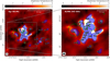 |
Fig. 1 Continuum emission toward Sgr B2(M) at 242 GHz. A close-up of the central part is presented in the right panel. The identified sources are shown as blue shaded polygons and are labeled with the corresponding source ID. The black points indicate the position of each core, described by Sánchez-Monge et al. (2017). The intensity color scale is shown in units of brightness temperature, and the synthesized beam of 0.″4 is in the lower left corner. The green ellipses are the H II regions identified by De Pree et al. (2015). |
2 Observations and data reduction
Sgr B2 was observed with the Atacama Large Millimeter/submillimeter Array ALMA (ALMA; ALMA Partnership 2015) during Cycle 2 in June 2014 and June 2015, using 34-36 antennas in an extended configuration with baselines in the range from 30 to 650 m, which results in an angular resolution of 0.″3 – 0.″7 (corresponding to ~3300 au). The observations were carried out in the spectral scan mode covering all of ALMA band 6 (211–275 GHz) with ten different spectral tunings, providing a resolution of 0.5–0.7 km s−1 across the full frequency band. The two sources Sgr B2(M) and Sgr B2(N) were observed in track-sharing mode, with phase centers at αJ2ooo = 17h47m20s.157, δJ2000 = −28°23′04.″53 for Sgr B2(M), and at αJ2000 = 17h47m19s.887, δJ2000 = −28°22′15.″76 for Sgr B2(N). Calibration and imaging were carried out with CASA1 version 4.4.0. Finally, all images were restored with a common Gaussian beam of 0.″4. Details of the observations, calibration and imaging procedures are described in Sánchez-Monge et al. (2017) and Schwörer et al. (2019).
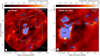 |
Fig. 2 Continuum emission toward Sgr B2(N) at 242 GHz. The right panel shows a close-up of the central part. The blue shaded polygons together with the corresponding source ID indicate the identified hot cores. The black points indicate the position of each core described by Sánchez-Monge et al. (2017). The intensity color scale is shown in units of brightness temperature, while the synthesized beam of 074 is indicated in the lower left corner. The green ellipses are the H II regions identified by De Pree et al. (2015). |
3 Data analysis
The spectra of each hot core and the corresponding surrounding envelope were modeled using the extended CASA Line Analysis Software Suite (XCLASS2; Möller et al. 2017) with additional extensions (Möller et al., in prep.). By solving the ID radiative transfer equation assuming local thermal equilibrium (LTE) conditions and an isothermal source, XCLASS enables the modeling and fitting of molecular lines
![Mathematical equation: $\matrix{ {{T_{{\rm{mb}}}}\left( \nu \right) = \sum\limits_{m,c \in i} {\left[ {\eta \left( {\theta _{{\rm{source}}}^{m,c}} \right)\left[ {{S^{m,c}}\left( \nu \right)\left( {1 - {e^{ - \tau _{{\rm{total}}}^{m,c}\left( \nu \right)}}} \right)} \right.} \right.} } \cr {\left. {\left. { + {I_{{\rm{bg}}}}\left( \nu \right)\left( {{e^{ - \tau _{{\rm{total}}}^{m,c}\left( \nu \right)}} - 1} \right)} \right]} \right]} \cr { + \left( {{I_{{\rm{bg}}}}\left( \nu \right) - {J_{{\rm{CMB}}}}} \right),} \cr } $](/articles/aa/full_html/2023/08/aa46903-23/aa46903-23-eq4.png) (1)
(1)
where the sums go over the indices m for molecule, and c for component. In Eq. (1), Tmb(v) represents the intensity in Kelvin, η(θm,c) the beam filling (dilution) factor, Sm,c(v) the source function (see Eq. (10)), and  the total optical depth of each molecule m and component c. Additionally, Ibg indicates the background intensity and JCMB the intensity of the cosmic microwave background. As Sgr B2(M) and (N) have high H2 densities (
 ), LTE conditions can be assumed (Mangum & Shirley 2015) and the kinetic temperature of the gas can be estimated from the rotation temperature: Trot ≈ Tkin For molecules, we assumed Gaussian line profiles, whereas Voigt line profiles were used for radio recombination lines (RRLs; see Sect. 3.1). Additionally, finite source size, dust attenuation, and optical depth effects were taken into account as well.
All molecular parameters (e.g., transition frequencies, Einstein A coefficients) were taken from an embedded SQLite database containing entries from the Cologne Database for Molecular Spectroscopy (CDMS; Müller et al. 2001, 2005) and the Jet Propulsion Laboratory database (JPL; Pickett et al. 1998) using the Virtual Atomic and Molecular Data Center (VAMDC; Endres et al. 2016). Additionally, the database used by XCLASS describes partition functions for more than 2500 molecules between 1.07 and 1000 K.
The contribution of each molecule is described by multiple emission and absorption components, where each component is specified by the source size θsource, the rotation temperature Trot, the column density Ntot, the line width Δv, and the velocity offset voffset from the source velocity (vLSR). Moreover, XCLASS offers the possibility to locate each component at a certain distance l along the line of sight. All model parameters can be fitted to observational data by using different optimization algorithms provided by the optimization package MAGIX (Möller et al. 2013). In order to reduce the number of fit parameters, the modeling can be done simultaneously with corresponding isotopologues and vibrationally excited states. The ratio with respect to the main species can be either fixed or used as an additional fit parameter (for details, see Möller et al. 2017).
3.1 Recombination lines
In addition to molecules, XCLASS can also analyze radio recombination lines. According to Quireza et al. (2006), who analyzed a large number of galactic H II regions, deviations from LTE are small, making LTE a reasonable assumption. Similar to molecules, the contribution of each RRL is described by a certain number of components, where each component is, in addition to source size θsource (in arcsec) and distance l (stacking parameter), defined by the electronic temperature Te (in K), the emission measure EM (in pc cm−6), the line width(s) Δυ (in km s−1), and the velocity offset voffset (in km s−1).
The optical depth of RRLs (in LTE) is given by (Gordon & Sorochenko 2002)
![Mathematical equation: $\matrix{ {{\tau _{{\rm{RRL}},\nu }} = \int {\kappa _{{n_1},{n_2},\nu }^{{\rm{ext}}}{\rm{d}}s} } \cr { = {{\pi {h^3}{e^2}} \over {{{\left( {2\pi {m_e}{k_{\rm{B}}}} \right)}^{3/2}}{m_e}c}} \cdot {\rm{EM}} \cdot {{n_1^2{f_{{n_1},{n_2}}}} \over {T_e^{3/2}}}} \cr { \times \exp \left[ {{{{Z^2}{E_{{n_1}}}} \over {{k_{\rm{B}}}{T_e}}}} \right]\left( {1 - {e^{ - h{\nu _{{n_1},{n_2}}}/{k_{\rm{B}}}{T_e}}}} \right){\phi _\nu }.} \cr } $](/articles/aa/full_html/2023/08/aa46903-23/aa46903-23-eq7.png) (2)
(2)
Here  indicates the oscillator strength
  , the transition frequency, n1 the main quantum number, and
  the energy of the lower state, which are taken from the embedded database. For each RRL the database contains oscillator strengths up to Δn = 6 (ζ-transitions) (i.e., all transitions of the RRL within the given frequency range up to ζ transitions are taken into account). In Eq. (2) the term φν represents the line profile function. XCLASS offers the possibility to use a Gaussian G(x) or a Voigt V(x, σ, γ) line profile function, which is a convolution of the Gaussian and the Lorentzian function (Gordon & Sorochenko 2002):
 (3)
(3)
Because the computation of the Voigt profile is computationally quite expensive, XCLASS uses the pseudo-Voigt profile  , which is an approximation of the Voigt profile V(x) using a linear combination of a Gaussian G(x) and a Lorentzian line profile function L(x), instead of their convolution. The mathematical definition of the normalized pseudoVoigt profile (i.e.,
  ) is given by
 (4)
(4)
with 0 < η < 1. There are several possible choices for the η parameter. XCLASS use the expression derived by Thompson et al. (1987),
 (5)
(5)
which is accurate to 1%. Here the expression
![Mathematical equation: $\matrix{ {f = \left[ {f_G^5 + 2.69269f_G^4{f_L} + 2.42843f_G^3f_L^2} \right.} \cr {{{\left. {\,\,\,\, + 4.47163f_G^2f_L^3 + 0.07842{f_G}f_L^4 + f_L^5} \right]}^{1/5}}} \cr } $](/articles/aa/full_html/2023/08/aa46903-23/aa46903-23-eq16.png) (6)
(6)
indicates the total full width at half maximum (FWHM), where fL and fG represents the Lorentzian and Gaussian full width at half maximum, respectively. The application of a Voigt line profile requires an additional parameter for each RRL and component. In addition to the Gaussian line width  , the Lorentzian line width
  (in km s−1) has to be specified as well. These line widths are related to the full widths at half maximum fL and fG by
 (7)
(7)
where  indicates the transition frequency of RRL m, component c, and transition t;
  the velocity offset; and υLSR the source velocity.
3.2 Free-free continuum
The hot plasma in H II regions gives rise to the emission of thermal bremsstrahlung, which causes a continuum opacity. The optical depth τff of this free-free contribution in terms of the classical electron radius  is given by (Beckert et al. 2000)
![Mathematical equation: $\matrix{ {{\tau _{{\rm{ff}}}} = {4 \over 3}{{\left( {{{2\pi } \over 3}} \right)}^{{1 \over 2}}}r_e^3Z{{Z_i^2{m^{3/2}}{c^5}} \over {\sqrt {{k_{\rm{B}}}{T_e}} h\,{\nu ^3}}}\left( {1 - {e^{ - {{h\nu } \over {{k_{\rm{B}}}Te}}}}} \right)\left\langle {{g_{{\rm{ff}}}}} \right\rangle \cdot {\rm{EM}}} \cr { = 1.13725 \cdot \left( {1 - {e^{ - {{h\nu } \over {{k_{\rm{B}}}Te}}}}} \right) \cdot \left\langle {{g_{{\rm{ff}}}}} \right\rangle } \cr {\,\,\,\, \times {{\left[ {{{{T_e}} \over K}} \right]}^{ - {1 \over 2}}}{{\left[ {{\nu \over {{\rm{GHz}}}}} \right]}^{ - 3}}\left[ {{{{\rm{EM}}} \over {{\rm{pc}}\,{\rm{c}}{{\rm{m}}^{ - 6}}}}} \right],} \cr } $](/articles/aa/full_html/2023/08/aa46903-23/aa46903-23-eq23.png) (8)
(8)
where Te indicates the electron temperature, EM the emission measure, and 〈gff〉 the thermal averaged free-free Gaunt coefficient. XCLASS makes use of the tabulated thermal averaged free-free Gaunt coefficients 〈gff〉 derived by van Hoof et al. (2015), which include relativistic effects as well. In order to model the free-free continuum contribution of a specific core we fitted the corresponding RRLs to obtain the electron temperatures Te and the emission measures EM (see Sect. 3.5).
3.3 Dust extinction
Extinction from dust is very important in Sgr B2 (see, e.g., Möller et al. 2021). Assuming that dust and gas are well mixed, the dust opacity τd(v) used by XCLASS is described by
![Mathematical equation: $\matrix{ {{\tau _d}\left( \nu \right) = {\tau _{d,{\rm{ref}}}} \cdot {{\left[ {{\nu \over {{\nu _{{\rm{ref}}}}}}} \right]}^\beta }} \cr { = \left[ {{N_{\rm{H}}} \cdot {\kappa _{{\nu _{{\rm{ref}}}}}} \cdot {m_{{{\rm{H}}_2}}} \cdot {1 \over {{\chi _{{\rm{gas}} - dust}}}}} \right] \cdot {{\left[ {{\nu \over {{\nu _{{\rm{ref}}}}}}} \right]}^\beta },} \cr } $](/articles/aa/full_html/2023/08/aa46903-23/aa46903-23-eq24.png) (9)
(9)
where NH indicates the hydrogen column density (in cm−2),  the dust mass opacity for a certain type of dust (in cm2 g−1, Ossenkopf & Henning 1994), and β the spectral index3. In addition, vref = 230 GHz represents the reference frequency for
  ,
,  the mass of a hydrogen molecule, and 1/χgas–dust the ratio of dust to gas, which is set here to 1/100 (Hildebrand 1983).
3.4 Local overlap
In line-crowded sources like Sgr B2(M) and (N), the line intensities from two neighboring lines that have central frequencies with (partly) overlapping width regions do not simply add up if at least one line is optically thick. Here photons emitted from one line were absorbed by the other line. XCLASS takes the local line overlap (described by Cesaroni & Walmsley 1991) from different components into account by computing an average source function Sl(v) at frequency ν and distance l
 (10)
(10)
where εl describes the emission and αl the absorption function,  the excitation temperature, and
  the optical depth of transition t and component c. Additionally, the optical depths of the individual lines included in Eq. (1) were replaced by their arithmetic mean at distance l,
![Mathematical equation: $\tau _{{\rm{total}}}^l\left( \nu \right) = \sum\limits_c {\left[ {\left[ {\sum\limits_t {\tau _t^c\left( \nu \right)} } \right] + \tau _d^c\left( \nu \right)} \right],} $](/articles/aa/full_html/2023/08/aa46903-23/aa46903-23-eq31.png) (11)
(11)
where the sums run over both components c and transitions t. Here  indicates the dust opacity, which was added as well. The iterative treatment of components at different distances, also takes nonlocal effects into account. The details of this procedure are described in Möller et al. (2021).
3.5 Fitting procedure
3.5.1 General model setup
In our analysis, we assume a two-layer model for all cores in Sgr B2(M) and (N), in which the first layer (hereafter the core layer) describes the contributions from the corresponding core. The second layer (hereafter the envelope layer) contains features from the local surrounding envelope of Sgr B2 and is located in front of the core layer. Here we assume that all components belonging to a layer have the same distance to the observer. Following Sánchez-Monge et al. (2017), a core is identified within the continuum emission maps of Sgr B2(M) and (N) if at least one closed contour (polygon) above the 3σ level is found (where σ indicates the rms noise level of the map of 8 mJy beam−1 for Sgr B2(M) and (N), respectively; see Figs. 1 and 2). The spectra for each core shown in Figs. 3 and 4 are obtained by averaging over all pixels contained in a polygon to improve the signal-to-noise ratio and the detection of weak lines.
As shown in Figs. 1 and 2, extended structures are clearly visible in addition to the identified compact sources; in other words, the dust is not concentrated in the cores only, but a non-negligible contribution is also contained in the envelope. Here we cannot distinguish between the contributions of the inner and outer envelope of Sgr B2. However, the outer envelope does not contribute significantly due to its much lower density. To obtain a reasonably consistent description of the continuum for each core spectrum, the dust parameters for each core and the local surrounding envelope have to be determined. In agreement with Sánchez-Monge et al. (2017), we assume a dust mass opacity of κ1300 μm = 1.11 cm2 g−1 (agglomerated grains with thin ice mantles in cores of densities 108 cm−3; Ossenkopf & Henning 1994) for both layers. For some hot cores, those for which we derive dust temperatures above 300 K, this may not be a good choice. Using a different dust mass opacity (e.g., κ1300 μm = 5.86 cm2 g−1; agglomerated grains without ice mantles in cores of densities 108 cm−3) results in hydrogen column densities that are lower by a factor of five.
In our analysis (see Fig. 5) we started by identifying molecules and, if contained, recombination lines in each core spectrum and determined a quantitative description of their respective contributions. Here we first used a phenomenological description of the corresponding continuum level and neglected dust and free-free contributions.
3.5.2 Envelope spectra
In the following we describe how we determined the dust parameters of the envelope by selecting pixels around each core that are not too close to another core or H II region4 (see Fig. 6). Here, we first selected points for each core that have the same distance to the core center, and then successively shifted outward those points that were still within the contour of the source or too close to a H II region. The spectra at these positions were used to compute an averaged envelope spectrum for each core (see Figs. 3 and 4), where we used STATCONT (Sánchez-Monge et al. 2018) to estimate the corresponding continuum level.
3.5.3 Dust parameters of the envelope
In order to compute the dust parameters for each envelope, we assumed that the gas temperature equals the dust temperature and estimated the gas temperature for each envelope by fitting CH3CN, H2CCO, H2CO, H2CS, HNCO, and SO in the corresponding spectra (see Fig. 7). These molecules were chosen because they show mostly isolated and nonblended transitions, and therefore they could be used to derive temperatures without requiring a full line survey analysis of the entire envelope spectrum. The final dust temperature for each envelope was computed by averaging over the obtained excitation temperatures. The corresponding hydrogen column density NH and spectral index β were determined by fitting the continuum level of each envelope spectrum using XCLASS.
3.5.4 Free-free parameters of the envelope
Some envelope spectra (A07, A09, A24, and A26 in Sgr B2(M)) contain RRLs, which we used to determine the free-free contribution to the corresponding continuum levels as well. The frequency ranges covered by our observation, contain two Hα (H29α and H30α), three Hβ (H36β, H37β H38β), three Ηγ (H41γ, H42γ, H43γ), four Hδ (Η44δ, Η46δ, Η47δ, Η48δ), five Hϵ (H47ϵ, H48ϵ, H49ϵ, H50ϵ, H51ϵ), and four Ηζ (Η50ζ, Η52ζ, Η53ζ, Η54ζ) transitions. Although the contributions of transitions with Δn ≥ 4 (δ-, ϵ-, and ζ-transitions) are very small, they can still help in determining the model parameters (electron temperature Te and the emission measure EM) because even very weak transitions contain useful information and provide additional constraints. In contrast to this procedure, we performed a full line survey analysis of each envelope spectrum containing RRLs taking local overlap into account (see Sect. 3.4) because the RRLs there contain nonnegligible admixtures of other molecules (see Fig. 8). In this analysis we started by modeling all molecules and RRLs using the new XCLASSGUI included in the extended XCLASS package, which offers the possibility to interactively model observational data and to describe molecules and recombination lines in LTE. The GUI can be used to generate synthetic spectra from input physical parameters, which can be overlaid on the observed spectra and/or fitted to the observations to obtain the best fit to the physical parameters. For all RRLs, we used a single emission component covering the full beam. Furthermore, for species where only one transition was included in the survey (e.g., CO and CS), a reliable quantitative description of their contribution was not possible. Since line overlap plays a major role for many sources, it was necessary to model the contributions of these molecules as well. Therefore, we fixed the excitation temperatures for components describing emission features to a value of 200 K5. For components describing absorption features, we assumed an excitation temperature of 2.7 K. In the next step we computed the average gas temperature from all identified molecules with more than one transition, where we took into account all components that describe emission features. After that, we performed one final fit, where all molecule and RRL parameters were fitted together with the hydrogen column density NH and spectral index β to achieve a self-consistent description of the molecular and recombination lines and the continuum level. Subsequently, we recomputed the average gas temperature to get the dust temperature of the envelope.
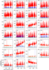 |
Fig. 3 Core (red line) and envelope (blue line) spectra for each core toward Sgr B2(M). The procedure used to calculate the envelope spectra is described in Sect. 3.5.2. The continuum level for each core spectrum is indicated by the orange dotted line, while the continuum level of each envelope spectrum is indicated by the green dotted line. |
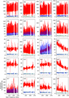 |
Fig. 4 Core (red line) and envelope (blue line) spectra for each core toward Sgr B2(N). The procedure used to calculate the envelope spectra is described in Sect. 3.5.2. The continuum level for each core spectrum is indicated by the orange dotted line, while the continuum level of each envelope spectrum is indicated by the green dotted line. |
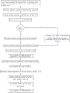 |
Fig. 5 Flow chart of fitting process. |
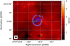 |
Fig. 6 Continuum emission toward Sgr B2(M) at 242 GHz around core A17 (blue shaded polygon). The positions used for the computation of the averaged envelope spectrum are indicated by blue crosses. The neighboring cores are indicated by blackcontours. The synthesized beam of 0.″4 is shown in the lower left corner. |
3.5.5 Continuum parameters of core
In the next step we estimated the continuum parameters for each core spectrum. Similarly to the procedure described above, we obtained the dust temperature for each core from the average gas temperature. We made use of the results of the analysis of the full molecular line survey. Here we modeled all RRLs with a single emission component, whose source size θcore is given by the diameter of a circle that has the same area Acore as the corresponding polygon describing the source6 (see Figs. 1 and 2), which means we determined the source size θcore (see Table 1) using
 (12)
(12)
For the temperature estimation we considered all the components of molecules that describe emission features in the corresponding core spectrum and that had more than one transition within the frequency ranges covered by the observation. Afterward, we used again XCLASS to derive the corresponding hydrogen column density NH and spectral index β, taking into account both the continuum contributions from the envelope layer and a possibly existing free-free contribution from the core layer (see Fig. 9). The obtained dust and free-free parameters for each layer and source are described in Tables 2–4. Additionally, we calculated the contribution y of each portion to the total continuum of the corresponding core spectrum by determining the ratio of the integrated intensity of each contribution and the total continuum. Here each contribution was calculated without taking the interaction with other contributions into account, which is why the ratios described in Tables 2–4 should be regarded as upper limits.
For some sources we were not able to derive a self-consistent description of the continuum of the corresponding core spectrum. For sources A10, A20, A25, and A27 in Sgr B2(M) and A07, A08, A10, A12, A13, and A20 in Sgr B2(N), we could not find RRLs despite negative slopes of the continuum levels. Additionally, the derived free-free parameters for source A16 in Sgr B2(N) cannot describe the observed slope. In addition, sources A18 in Sgr B2(M) and A11 in Sgr B2(N) show positive slopes that cannot be explained by optically thin dust emissions. As mentioned by Sánchez-Monge et al. (2017), for some faint sources the slope of the continuum levels might be falsified by calibration issues and the frequency-dependent filtering out of extended emission. For all sources where a self-consistent description of the core continuum was not possible, we applied a phenomenological description of the continuum and used averaged dust parameters for the core layers in sources in Sgr B2(M) and Sgr B2(N), respectively.
3.5.6 Errors of continuum parameters
The errors of the continuum parameters described in Tables 2–4 are derived by two different methods. The errors of the dust temperatures for spectra without RRLs describe the standard errors of the corresponding means, while the errors of the other parameters were estimated using the emcee7 package (Foreman-Mackey et al. 2013), which implements the affine-invariant ensemble sampler of Goodman & Weare (2010), to perform a Markov chain Monte Carlo (MCMC) algorithm approximating the posterior distribution of the model parameters by random sampling in a probabilistic space. Here, the MCMC algorithm starts at the estimated maximum of the likelihood function, which is the continuum model parameters described in Tables 2–4, and draws 30 samples (walkers) of model parameters from the likelihood function in a small ball around the a priori preferred position. For each parameter we used 500 steps to sample the posterior. The probability distribution and the corresponding highest posterior density (HPD) interval of each continuum parameter were calculated afterward. Details of the HPD interval are described in Möller et al. (2021). In order to get a more reliable error estimation, the errors for the hydrogen column densities and emission measures are calculated on log scale (i.e., these parameters are converted to their log10 values before applying the MCMC algorithm) and converted back to linear scale after finishing the error estimation procedure. For most sources, the log10 errors of the hydrogen column densities and spectral indices are tiny, so the linear values are usually on the order of one. Finally the errors of the ratios γ are calculated using the continuum parameters, where each parameter is reduced (enhanced) by the corresponding left (right) error value.
The posterior distributions of the continuum parameters of core A17 in Sgr B2(M) are shown in Fig. 10; the distributions for the other cores are shown in Appendix A. For all histograms we find a unimodal distribution, i.e. that the associated parameters are uniquely determined.
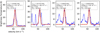 |
Fig. 7 Selected transitions of HNCO (red lines) contained in the envelope spectrum (blue lines) around core A08 in Sgr B2(M). The gray dashed line indicates the source velocity υlsr = 64 km s−1 of Sgr B2. |
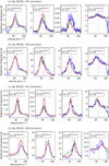 |
Fig. 8 Selected RRLs in the envelope spectra around core A07 (a), A09 (b), A24 (c), and A26 (d) in Sgr B2(M). The observational data is indicated by the blue line, the pure RRL contribution by the red line, and the model spectrum taking all identified molecules into account by the dashed green line. The vertical gray dashed line indicates the source velocity of Sgr B2(M). |
Physical parameters for each source in Sgr B2(M) and Sgr B2(N).
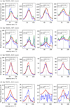 |
Fig. 9 Selected RRLs in core spectra of A01 (a), A07 (b), and A16 (c) in Sgr B2(M) and A16 (d) in Sgr B2(N). The observational data is described by the blue line, the pure RRL contribution by the red line, and the model spectrum taking all identified molecules into account by the dashed green line. The vertical gray dashed line indicates the source velocity of Sgr B2(M). |
Dust and free-free parameters for each envelope around sources in Sgr B2(M).
Dust and free-free parameters for each core in Sgr B2(M).
4 Results and discussion
4.1 Results
In the two regions, Sgr B2(M) and Sgr B2(N), most of the cores and their local envelopes are dominated by the contribution of thermal dust, where the dense dust-dominated cores are optically thick toward the center and optically thin in the outer regions (see Figs. 11 and 12). The greater number of H II regions in Sgr B2(M) cause strong thermal free-free emissions, which for some cores are the dominant continuum contributions to the total continuum levels. However, we also detect ionized gas localized between the sources, as we found in the envelope around cores A09 and A26 in Sgr B2(M).
4.1.1 Results of Sgr B2(M)
For local envelopes around the hot cores in Sgr B2(M) we found only a small variation in the dust parameters except for those envelopes containing RRLs (A07, A09, A24, and A26). The dust temperatures vary between 46 K (A19) and 88 K (A08) for envelopes whose spectra do not contain RRLs. For envelopes where free-free ionized gas emission has been found, the dust temperatures are in the range of 50 K (A24) and 162 K (A26). Additionally, the envelope around the central core A01 shows the highest hydrogen column density of 1.1 × 1025 cm−2, while the lowest hydrogen column densities are found for envelopes containing RRLs. For the majority of spectra we find spectral dust indices of β = 0.1 (α = 2.1) (A05, A08, A10, A11, A13, A14, A17, A18, A19, A21, A22, A23, A25), which are associated with optically thick dust emission (see, e.g., Schnee et al. 2014, Reach et al. 2015). For core A03, we derive an index of β = 2.0 (a = 4.0), which indicates optically thin dust emission. Envelopes containing free-free emission in their spectra have spectral dust indices between 0.2 and 0.4 (i.e., moderate optically thick dust emission). The contributions of the dust emission from the envelopes to the total continua observed toward the hot cores vary between 5.4 (A03) and 32.4% (A14). From the RRLs we obtain electronic temperatures between 2781 (A09) and 5817 Κ (A07), finding no correlation with dust temperatures. The corresponding emission measures are located within a small range between 8.8 × 10⁶ (pc cm−6) (A07) and 2.2 × 10⁷ (pc cm−6) (A24). The free-free emissions in the envelopes contribute almost nothing to the observed continuum and range from 0.5 (A07) to 2.2% (A26). Eight hot core spectra in Sgr B2(M) contain RRLs. For two other sources (A09, A26) we could not detect RRLs in the corresponding core spectra, although RRLs are found in their envelopes, which may be due to the fact that there is ionized gas localized between the sources and that we used averaged core spectra (see, e.g., Fig. 6, where possible contributions from individual pixels with a small RRL contribution were averaged out). For example, the polygon used to calculate the averaged core spectrum of A26 contains a small H II region identified by De Pree et al. (2015; see Fig. 1), but we could not detect any RRLs in the corresponding core spectrum. On the other hand, the identification of RRLs in the core spectrum of A17 in Sgr B2(M) is remarkable because De Pree et al. (2015) do not describe a H II region in the vicinity of this source. The hot cores in Sgr B2(M) have dust temperatures ranging from 195 (A26) to 342 Κ (A01), but unlike in the envelope spectra, we do not find a general correlation between cores containing RRLs and high dust temperatures, which again may be due to the use of averaged core spectra. Moreover, we obtain the highest hydrogen column density not for the central core A01, as Sánchez-Monge et al. (2017), but for core A03. This discrepancy could be due to the fact that, unlike Sánchez-Monge et al. (2017), we decompose the contributions from the envelope and core, where the envelope around core A01 has the highest hydrogen column density of all envelopes in Sgr B2(M). Furthermore, the continuum of core A01 contains strong free ionized gas emissions. In contrast to the envelopes, the majority of core spectra shows spectral dust indices above 0.4. Only three cores have spectral indices of β = 0.0 (α = 0.0). Half of all cores (A01, A04, A07, and A08) containing RRLs have spectral indices above 1.0, which are associated with optically thin dust emission. For cores whose spectra do not contain RRLs and for which we could derive a self-consistent description of the continuum level, we obtain approximately the same spectral indices as Sánchez-Monge et al. (2017).
The obtained electronic temperatures Te show a large variation between 3808 (A01) and 23 779 Κ (A17). Although electronic temperatures above 10 000 Κ are unusual for H II regions (Zuckerman et al. 1967, Gordon & Sorochenko 2002), the temperatures agree quite well with those derived by Quireza et al. (2006), where temperatures between 1850 and 21 810 Κ were found using high-precision radio recombination line and continuum observations of more than 100 H II regions in the Galactic disk. Taking non-LTE effects into account, Mehringer et al. (1995) derived an electronic temperature of Te = 23 700 Κ toward a source in Sgr B2(M), which is very close to the LTE temperature we determined for source A17. Additionally, Quireza et al. (2006) identified a Galactic H II region (G220.508–2.8) with an electronic temperature of Te = 21 810 K. Furthermore, the error estimation for A17 (see Fig. 10) shows that the best description of the free-free contribution occurs at the indicated temperature. Although we cannot rule out the possibility that the slope of the continuum level of core A17 is affected by interferometric filtering, this high temperature seems to actually exist, but it is unclear what mechanism heats the gas to such high temperatures. The electron temperature of a H II region in thermal equilibrium is determined by the balance of competing heating and cooling mechanisms. Among others, the electronic temperature Te can be influenced by the effective temperature of the ionizing star or by the electron density, which inhibits cooling and increases Te by collisional excitation in the high electron density H II regions. Additionally, Te is affected by the dust grains, which are involved in heating and cooling in complex ways (see, e.g., Mathis 1986; Baldwin et al. 1991; Shields & Kennicutt 1995). Photoelectric heating occurs due to the ejection of electrons from the dust grains, while the gas is cooled by collisions of fast particles with the grains. Furthermore, the electron temperature decreases with distance from the star because the field of ionizing radiation is attenuated by dust grains. However, the electron temperature also increases when coolants are depleted at the dust grains. According to Dyson & Williams (1980), photoionization is not able to heat the material to such a high temperature unless there is a strong depletion of metals in this region compared to other H II regions in Sgr B2. Since heavy elements cool photoionized gas, the electron temperatures of H II regions are directly related to the abundance of the heavy elements. A low electron temperature Te corresponds to a higher heavy element abundance due to the higher cooling rate and vice versa. Another possibility is that the heating is caused by a non-equilibrium situation at the edge of the expanding H II region. The electronic temperatures of the other cores correspond quite well to those obtained by Mehringer et al. (1993), suggesting that the metal abundance in most cores of Sgr B2 is similar to that of Orion.
The corresponding emission measures ranges from 4.7 × 10⁸ (pc cm−6) (A17) to 4.4 × 10⁹ (pc cm−6) (A01). The free-free contributions to the total continuum levels vary between 15.7 and 75.8%, where the high contributions are caused by the fact that seven of the hot cores in Sgr B2(M) contain one or more H II regions (see Fig. 1), while core A17 was not associated with H II regions before, which may be caused by the strong dust contribution (see Fig. 13).
Dust and free-free parameters for each source in Sgr B2(N).
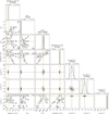 |
Fig. 10 Corner plot (Foreman-Mackey 2016) showing the 1D and 2D projections of the posterior probability distributions of the continuum parameters of core A17, in Sgr B2(M). At the top of each column the probability distribution for each free parameter is shown together with the 50% quantile (median) and the corresponding left and right errors. The left and right dashed lines indicate the lower and upper limits of the corresponding HPD interval, respectively. The blue line indicates the median of the distribution. The dashed orange lines indicate the parameter values of the best fit. The plots in the lower left corner describe the projected 2D histograms of two parameters. For a better estimation of the errors, the error of the hydrogen column density and the emission measure on log10 scale are determined and use the velocity offset (υoff) related to the source velocity of υLSR = 64 km s−1. |
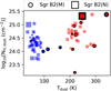 |
Fig. 11 Derived dust temperatures and hydrogen column densities for each envelope (blue) and core (red) layer in Sgr B2(M) (circles) and (N) (squares). Layers containing RRLs are indicated by a black border. The size of each scatter point corresponds to the corresponding source size. |
 |
Fig. 12 Derived dust temperatures and spectral indices for each envelope (blue) and core (red) layer in Sgr B2(M) (circles) and (N) (squares). Layers containing RRLs are indicated by a black border. The size of each scatter point corresponds to the corresponding source size. |
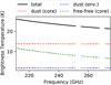 |
Fig. 13 Continuum contributions to core A17 in Sgr B2(M). Each contribution is computed without taking the interaction with other contributions into account. |
4.1.2 Results of Sgr B2(N)
As in Sgr B2(M), we found only a small variation in the dust parameters for the local envelopes around the hot cores in Sgr B2(N). The dust temperatures are located in a range between 35 Κ (A02) and 86 Κ (A15), while the column densities vary between 5.1 × 1023 cm−2 (A12) and 1.0 × 1025 cm−2 (A01). As for the envelope spectra around sources in Sgr B2(M), we find spectral dust indices for most of the envelopes (A04, A08, A09, A10, A12, A13, A14, A15, A18, A19, and A20) in Sgr B2(N) of 0.1. The highest dust index of β = 2.5 (α = 4.5) is found for the envelope around core A07. In contrast to Sgr B2(M), we did not find RRLs in the envelope spectra in Sgr B2(N). The dust emissions from the envelopes contribute between 6.6 (A03) and 71.2% (A17) to the total continuum level. The strong contribution of the envelope around source A17 shows that the contribution of the envelope is indispensable for a realistic modeling of a sources with low continuum levels. For the hot cores in Sgr B2(N) we derived dust temperatures between 190 (A09) and 282 Κ (A 14), where the high core dust temperature of source A 19 is noteworthy because this source is not associated with a H II region. However, we cannot exclude an influence of interferometric filtering on molecular lines used for temperature estimation. The column densities alter between 1.3 × 1024 (A17) and 2.1 × 1025 cm−2 (A01) and the spectral index between β = −0.1 (α = 1.9) (A 07) and β = 2.5 (α = 4.5) (A01). Only two cores contain RRLs with electronic temperatures of 9877 (A01) and 9921 Κ (A16). The corresponding emission measures are located in a range between 1.0 × 10⁸ (A 16) and 3.9 × 10⁸ (pc cm−6) (A01), which is almost an order of magnitude lower than the highest emission measure for core A01 in Sgr B2(M). For A01 the free-free contribution is 10.5%.
In the following we present in more detail the results obtained from the fitting toward the cores of Sgr B2(M) and (N).
4.2 Physical properties of the continuum sources
In Table 1, we summarize the physical parameters derived from the continuum parameters described above. Here we compute the (dust and gas) masses for each source determined from the expression (Hildebrand 1983)
 (13)
(13)
where Sv is the flux density at 242 GHz, D is the distance (8.34 kpc for Sgr B2),  is the Planck function at a core dust temperature
  , and κν is the absorption coefficient per unit of total mass (gas and dust) density. Assuming a spherical and homogeneous core, we use the following expression to estimate the hydrogen density
  from the hydrogen column density
  :
:
 (14)
(14)
Here dcore = D · θcore indicates the diameter and θcore the corresponding source size of the source. The electron density  is computed in a similar way using the derived emission measure EMcore,
 (15)
(15)
where we assume spherical and homogeneous H II regions.
The ionized gas mass  is estimated using the expression
 (16)
(16)
where mp indicates the proton mass. Finally, we calculate the number of ionizing photons per second  (Schmiedeke et al. 2016),
 (17)
(17)
where we assume a Strömgren sphere. Here  and
and  are the rate coefficients for recombinations to all levels and to the ground state, respectively. The term (
 ) describes the recombination coefficient to level 2 or higher, and can be described using the expression derived by Rubin (1968),
 (18)
(18)
which approximates the recombination coefficient given by Seaton (1959) for electron temperatures Te.
Unlike other cores containing H II regions, cores A15 and A24 in Sgr B2(M) each approximately match in position and size a single H II region identified by De Pree et al. (2015). In the following we estimate the age of these H II regions. We start by calculating the initial Strömgren radius (RSt) of a H II region, which is given by (Spitzer 1968)
![Mathematical equation: ${R_{{\rm{St}}}} = {\left( {{3 \over {16\,\pi \left( {\tilde \beta - {{\tilde \beta }_1}} \right)}} \cdot {{\dot N_i^{{\rm{core}}}} \over {{{\left[ {n_{{{\rm{H}}_2}}^{{\rm{core}}}} \right]}^2}}}} \right)^{{1 \mathord{\left/ {\vphantom {1 3}} \right. \kern-\nulldelimiterspace} 3}}},$](/articles/aa/full_html/2023/08/aa46903-23/aa46903-23-eq346.png) (19)
(19)
where  indicates the number of ionizing photons per second, Eq. (17);
  the hydrogen density, Eq. (14); and (
 ) the recombination coefficient, Eq. (18).
Assuming expansion into a homogeneous molecular cloud, the dynamical age of both regions can now be computed by using the following expansion equation (Spitzer 1968, Dyson & Williams 1980):
![Mathematical equation: ${t_{\exp }} = {4 \over 7}{{{R_{{\rm{St}}}}} \over {{c_s}}}\left[ {{{\left( {{{{r^{{\rm{core}}}}} \over {{R_{{\rm{St}}}}}}} \right)}^{{7 \mathord{\left/ {\vphantom {7 4}} \right. \kern-\nulldelimiterspace} 4}}} - 1} \right].$](/articles/aa/full_html/2023/08/aa46903-23/aa46903-23-eq350.png) (20)
(20)
Here rcore = dcore/2 describes the radius of the H II region and RSt the Strömgren radius, Eq. (19). In addition, cs indicates the isothermal sound speed, which is given by (Draine 2011)
 (21)
(21)
where mH is the hydrogen atomic mass.
Additionally, we compute the ratio of electron to molecular pressure (Tsuboi et al. 2019),
 (22)
(22)
where  represents the electron density, Eq. (15);
  the hydrogen density, Eq. (14);
  the dust; and
  the electronic temperature. A ratio higher than one means that the corresponding H II region is in the expansion phase since the pressure of the ionized gas exceeds the pressure of the neutral gas.
Compared to Sánchez-Monge et al. (2017), we find much lower dust and gas masses (between 27 and 57% of their masses), which is due to our elevated dust temperatures. Sánchez-Monge et al. (2017) assume a dust temperature of 100 K, while our core dust temperatures range from 190 to 342 K. However, the mass distribution of the most massive cores is almost unchanged for both regions. In addition, we obtain reduced H2 volume densities  for most sources in Sgr B2(M) and (N). For the central sources, our densities are in the range between 4 and 153% of the previous analysis results, while the volume densities for some outlying sources, especially in Sgr B2(M), exceed the results of Sánchez-Monge et al. (2017) by a factor of up to five (A26). These discrepancies are due to, among other factors, the different sizes of the sources used in our analysis compared to those described in Sánchez-Monge et al. (2017). Nevertheless, the highest hydrogen density, which we determine in our analysis is on the order of 108 cm−3, which corresponds to 106 M⊙ pc−3, still one order of magnitude higher than the typical stellar density found in super star clusters (e.g., ~105 M⊙ pc−3; Portegies Zwart et al. 2010).
Finally, we calculate the physical parameters of the ionized gas for the sources in which we identified RRLs. In Sgr B2(M) we find RRLs in all sources except A02, where Sánchez-Monge et al. (2017) had also found contributions from ionized gas. This is quite different for Sgr B2(N), in which we find RRLs only for the central source A01. In all other sources that were connected with H II regions by Sánchez-Monge et al. (2017), we do not find RRLs. However, we identify RRLs in A16 that were not associated with ionized gas by Sánchez-Monge et al. (2017). The H II regions we identify fit very well with the results of De Pree et al. (2015) for both regions. According to De Pree et al. (2015), only sources A01, A10, and A16 in Sgr B2(N) contain H II regions. The electron densities ne vary between 47 and 211% of the values derived from Sánchez-Monge et al. (2017); the differences are due to the different analysis techniques. In contrast to Sánchez-Monge et al. (2017), who found the highest electron density for core A01 in Sgr B2(M), we obtain the highest electron density for core A24, which is associated with a single bright H II region (see Fig. 1). All other cores containing RRLs show comparable densities. For core A15 and A24 in Sgr B2(M) we also determine the age of the corresponding H II region (A15: 3100 yr, A24: 7000 yr), which are comparable to the results obtained by Meng et al. (2022). Additionally, the gas pressure ratio of the observed ionized gas and the observed ambient molecular gas is close to unity for A24, which indicates that the pressure-driven expansion for the corresponding H II region is coming to a halt, while for core A15 we find a remarkable pressure-driven expansion for this H II region.
5 Conclusions
Many of the hot cores identified by Sánchez-Monge et al. (2017) include large amounts of dust. In addition, some cores contain one or more H II regions. In this work, which is the first of two papers on the complete analysis of the full spectral line surveys toward these hot cores, we quantify the dust and, if contained, the free-free contributions to the continuum levels. In contrast to previous analyses, we derived the corresponding parameters here not only for each core, but also for their local surrounding envelope, and determined their physical properties. Especially for some outlying sources, the contributions of these envelopes are not negligible. In general, the distribution of RRLs we found in the core spectra fits well with the distribution of H II regions described by De Pree et al. (2015). Only for core A02 in Sgr B2(M) and A10 in Sgr B2(N) we cannot identify RRLs in the corresponding spectra, although H II regions are contained in these sources. Additionally, we found RRLs in core A17 of Sgr B2(M), even though no H II region is known to be nearby. The average dust temperature for envelopes around sources in Sgr B2(M) is 73 K; in Sgr B2(N), however, we obtain only 59 K, which may be caused by the enhanced number of H II region in Sgr B2(M) compared to (N). For the cores we obtain average dust temperatures around 236 K (Sgr B2(M)) and 225 K (Sgr B2(N)), and we see no correlations between occurrence of RRLs and enhanced dust temperatures, although one would expect this in the presence of ionized gas. For the average hydrogen column densities we get 2.5 × 1024 cm−2 (2.6 × 1024 cm−2) for the envelopes and 7.8 × 1024 cm−2 (6.1 × 1024 cm−2) for Sgr B2(M) and (N), respectively. The derived electronic temperatures are located in a range between 2781 and 9921 K, while the two cores show electronic temperatures of 15 214 and 23 779 K. The highest emission measures in Sgr B2(M) are found in cores A01 and A24, while the two cores in Sgr B2(N) containing RRLs have almost the same emission measure. In Sgr B2(M), the three inner sources are the most massive, whereas in Sgr B2(N) the innermost core A01 dominates all other sources in mass and size. This analysis of the dust and ionized gas contribution to the continuum emission enables a full detailed analysis of the spectral line content which will be presented in a following paper (Möller et al., in prep.).
Acknowledgements
This work was supported by the Deutsche Forschungsgemeinschaft (DFG) through grant Collaborative Research Centre 956 (subproject A6 and C3, project ID 184018867) and from BMBF/Verbundforschung through the projects ALMA-ARC 05A14PK1 and ALMA-ARC 05A20PK1. A.S.M. acknowledges support from the RyC2021-032892-I grant funded by MCIN/AEI/10.13039/501100011033 and by the European Union ‘Next Genera-tionEU’/PRTR, as well as the program Unidad de Excelencia Maria de Maeztu CEX2020-001058-M. This paper makes use of the following ALMA data: ADS/JAO.ALMA#2013.1.00332.S. ALMA is a partnership of ESO (representing its member states), NSF (USA) and NINS (Japan), together with NRC (Canada), MOST and ASIAA (Taiwan), and KASI (Republic of Korea), in cooperation with the Republic of Chile. The Joint ALMA Observatory is operated by ESO, AUI/NRAO and NAOJ.
Appendix A Error estimation
A.1 Error estimation of continuum parameters for cores in Sgr B2(M)
Corner plots (Foreman-Mackey 2016) showing the 1D and 2D projections of the posterior probability distributions of the continuum parameters of each core in Sgr B2(M). At the top of each column the probability distribution for each free parameter is shown together with the value of the best fit and the corresponding left and right errors. The left and right dashed lines indicate the lower and upper limits of the corresponding highest posterior density (HPD) interval, respectively. The dashed line in the middle indicates the mode of the distribution. The blue lines indicate the parameter values of the best fit. The plots in the lower left corner show the projected 2D histograms of two parameters and the contours the HPD regions. In order to get a better estimation of the errors, we determine the error of the hydrogen column density and the emission measure on log scale and use the velocity offset (voff) related to the source velocity of vLSR = 64 km s−1.
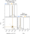 |
Figure A.1 Corner plot for source A01 in Sgr B2(M), envelope layer. |
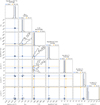 |
Figure A.2 Corner plot for source A01 in Sgr B2(M), core layer. |
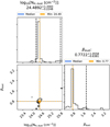 |
Figure A.3 Corner plot for source A02 in Sgr B2(M), envelope layer. |
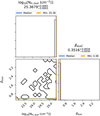 |
Figure A.4 Corner plot for source A02 in Sgr B2(M), core layer. |
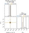 |
Figure A.5 Corner plot for source A03 in Sgr B2(M), envelope layer. |
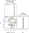 |
Figure A.6 Corner plot for source A03 in Sgr B2(M), core layer. |
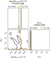 |
Figure A.7 Corner plot for source A04 in Sgr B2(M), envelope layer. |
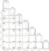 |
Figure A.8 Corner plot for source A04 in Sgr B2(M), core layer. |
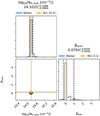 |
Figure A.9 Corner plot for source A05 in Sgr B2(M), envelope layer. |
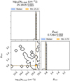 |
Figure A.10 Corner plot for source A05 in Sgr B2(M), core layer. |
 |
Figure A.11 Corner plot for source A06 in Sgr B2(M), envelope layer. |
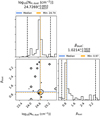 |
Figure A.12 Corner plot for source A06 in Sgr B2(M), core layer. |
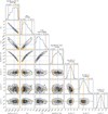 |
Figure A.13 Corner plot for source A07 in Sgr B2(M), envelope layer. |
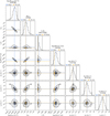 |
Figure A.14 Corner plot for source A07 in Sgr B2(M), core layer. |
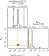 |
Figure A.15 Corner plot for source A08 in Sgr B2(M), envelope layer. |
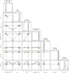 |
Figure A.16 Corner plot for source A08 in Sgr B2(M), core layer. |
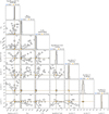 |
Figure A.17 Corner plot for source A09 in Sgr B2(M), envelope layer. |
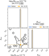 |
Figure A.18 Corner plot for source A09 in Sgr B2(M), core layer. |
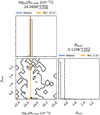 |
Figure A.19 Corner plot for source A10 in Sgr B2(M), envelope layer. |
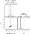 |
Figure A.20 Corner plot for source A11 in Sgr B2(M), envelope layer. |
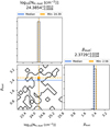 |
Figure A.21 Corner plot for source A11 in Sgr B2(M), core layer. |
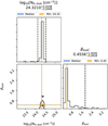 |
Figure A.22 Corner plot for source A12 in Sgr B2(M), envelope layer. |
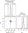 |
Figure A.23 Corner plot for source A12 in Sgr B2(M), core layer. |
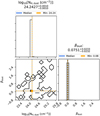 |
Figure A.24 Corner plot for source A13 in Sgr B2(M), envelope layer. |
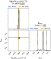 |
Figure A.25 Corner plot for source A13 in Sgr B2(M), core layer. |
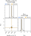 |
Figure A.26 Corner plot for source A14 in Sgr B2(M), envelope layer. |
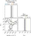 |
Figure A.27 Corner plot for source A14 in Sgr B2(M), core layer. |
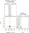 |
Figure A.28 Corner plot for source A15 in Sgr B2(M), envelope layer. |
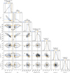 |
Figure A.29 Corner plot for source A15 in Sgr B2(M), core layer. |
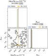 |
Figure A.30 Corner plot for source A16 in Sgr B2(M), envelope layer. |
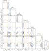 |
Figure A.31 Corner plot for source A16 in Sgr B2(M), core layer. |
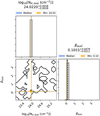 |
Figure A.32 Corner plot for source A17 in Sgr B2(M), envelope layer. |
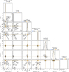 |
Figure A.33 Corner plot for source A17 in Sgr B2(M), core layer. |
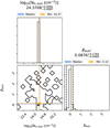 |
Figure A.34 Corner plot for source A18 in Sgr B2(M), envelope layer. |
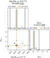 |
Figure A.35 Corner plot for source A19 in Sgr B2(M), envelope layer. |
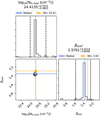 |
Figure A.36 Corner plot for source A19 in Sgr B2(M), core layer. |
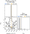 |
Figure A.37 Corner plot for source A20 in Sgr B2(M), envelope layer. |
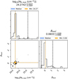 |
Figure A.38 Corner plot for source A21 in Sgr B2(M), envelope layer. |
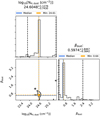 |
Figure A.39 Corner plot for source A21 in Sgr B2(M), core layer. |
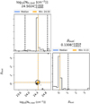 |
Figure A.40 Corner plot for source A22 in Sgr B2(M), envelope layer. |
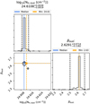 |
Figure A.41 Corner plot for source A22 in Sgr B2(M), core layer. |
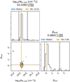 |
Figure A.42 Corner plot for source A23 in Sgr B2(M), envelope layer. |
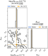 |
Figure A.43 Corner plot for source A23 in Sgr B2(M), core layer. |
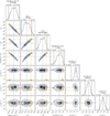 |
Figure A.44 Corner plot for source A24 in Sgr B2(M), envelope layer. |
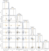 |
Figure A.45 Corner plot for source A24 in Sgr B2(M), core layer. |
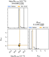 |
Figure A.46 Corner plot for source A25 in Sgr B2(M), envelope layer. |
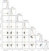 |
Figure A.47 Corner plot for source A26 in Sgr B2(M), envelope layer. |
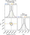 |
Figure A.48 Corner plot for source A26 in Sgr B2(M), core layer. |
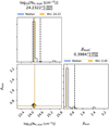 |
Figure A.49 Corner plot for source A27 in Sgr B2(M), envelope layer. |
A.2 Error estimation of continuum parameters for cores in Sgr B2(N)
The corner plots (Foreman-Mackey 2016) here show the 1D and 2D projections of the posterior probability distributions of the continuum parameters of each core in Sgr B2(N). At the top of each column the probability distribution for each free parameter is shown together with the value of the best fit and the corresponding left and right errors. The left and right dashed lines indicate the lower and upper limits of the corresponding highest posterior density (HPD) interval, respectively. The dashed line in the middle indicates the mode of the distribution. The blue lines indicate the parameter values of the best fit. The plots in the lower left corner show the projected 2D histograms of two parameters and the contours the HPD regions. In order to get a better estimation of the errors, we determine the error of the hydrogen column density and the emission measure on log scale and use the velocity offset (voff) related to the source velocity of VLSR = 64 km s−1.
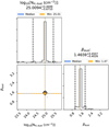 |
Figure A.50 Corner plot for source A01 in Sgr B2(N), envelope layer. |
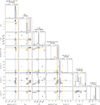 |
Figure A.51 Corner plot for source A01 in Sgr B2(N), core layer. |
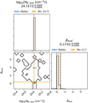 |
Figure A.52 Corner plot for source A02 in Sgr B2(N), envelope layer. |
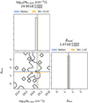 |
Figure A.53 Corner plot for source A02 in Sgr B2(N), core layer. |
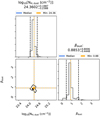 |
Figure A.54 Corner plot for source A03 in Sgr B2(N), envelope layer. |
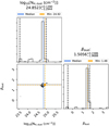 |
Figure A.55 Corner plot for source A03 in Sgr B2(N), core layer. |
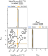 |
Figure A.56 Corner plot for source A04 in Sgr B2(N), envelope layer. |
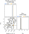 |
Figure A.57 Corner plot for source A04 in Sgr B2(N), core layer. |
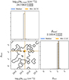 |
Figure A.58 Corner plot for source A05 in Sgr B2(N), envelope layer. |
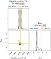 |
Figure A.59 Corner plot for source A05 in Sgr B2(N), core layer. |
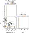 |
Figure A.60 Corner plot for source A06 in Sgr B2(N), envelope layer. |
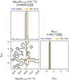 |
Figure A.61 Corner plot for source A06 in Sgr B2(N), core layer. |
 |
Figure A.62 Corner plot for source A07 in Sgr B2(N), envelope layer. |
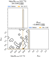 |
Figure A.63 Corner plot for source A07 in Sgr B2(N), core layer. |
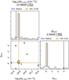 |
Figure A.64 Corner plot for source A08 in Sgr B2(N), envelope layer. |
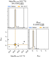 |
Figure A.65 Corner plot for source A09 in Sgr B2(N), envelope layer. |
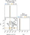 |
Figure A.66 Corner plot for source A09 in Sgr B2(N), core layer. |
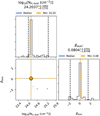 |
Figure A.67 Corner plot for source A10 in Sgr B2(N), envelope layer. |
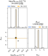 |
Figure A.68 Corner plot for source A11 in Sgr B2(N), envelope layer. |
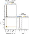 |
Figure A.69 Corner plot for source A12 in Sgr B2(N), envelope layer. |
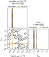 |
Figure A.70 Corner plot for source A13 in Sgr B2(N), envelope layer. |
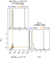 |
Figure A.71 Corner plot for source A14 in Sgr B2(N), envelope layer. |
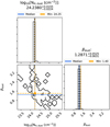 |
Figure A.72 Corner plot for source A14 in Sgr B2(N), core layer. |
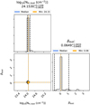 |
Figure A.73 Corner plot for source A15 in Sgr B2(N), envelope layer. |
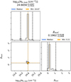 |
Figure A.74 Corner plot for source A15 in Sgr B2(N), core layer. |
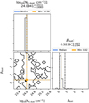 |
Figure A.75 Corner plot for source A16 in Sgr B2(N), envelope layer. |
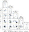 |
Figure A.76 Corner plot for source A16 in Sgr B2(N), core layer. |
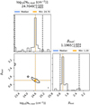 |
Figure A.77 Corner plot for source A17 in Sgr B2(N), envelope layer. |
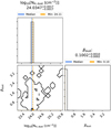 |
Figure A.78 Corner plot for source A17 in Sgr B2(N), core layer. |
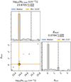 |
Figure A.79 Corner plot for source A18 in Sgr B2(N), envelope layer. |
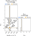 |
Figure A.80 Corner plot for source A18 in Sgr B2(N), core layer. |
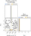 |
Figure A.81 Corner plot for source A19 in Sgr B2(N), envelope layer. |
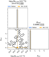 |
Figure A.82 Corner plot for source A19 in Sgr B2(N), core layer. |
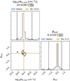 |
Figure A.83 Corner plot for source A20 in Sgr B2(N), envelope layer. |
References
- ALMA Partnership (Fomalont, E.B., et al.) 2015, ApJ, 808, L1 [NASA ADS] [CrossRef] [Google Scholar]
- Baldwin, J. A., Ferland, G. J., Martin, P. G., et al. 1991, ApJ, 374, 580 [Google Scholar]
- Beckert, T., Duschl, W. J., & Mezger, P. G. 2000, A&A, 356, 1149 [NASA ADS] [Google Scholar]
- Belloche, A., Müller, H. S. P., Menten, K. M., Schilke, P., & Comito, C. 2013, A&A, 559, A47 [NASA ADS] [CrossRef] [EDP Sciences] [Google Scholar]
- Cesaroni, R., & Walmsley, C. M. 1991, A&A, 241, 537 [NASA ADS] [Google Scholar]
- Cummins, S. E., Linke, R. A., & Thaddeus, P. 1986, ApJS, 60, 819 [NASA ADS] [CrossRef] [Google Scholar]
- de Pree, C. G., Gaume, R. A., Goss, W. M., & Claussen, M. J. 1995, ApJ, 451, 284 [NASA ADS] [CrossRef] [Google Scholar]
- de Pree, C. G., Gaume, R. A., Goss, W. M., & Claussen, M. J. 1996, ApJ, 464, 788 [NASA ADS] [CrossRef] [Google Scholar]
- De Pree, C. G., Peters, T., Mac Low, M. M., et al. 2014, ApJ, 781, L36 [NASA ADS] [CrossRef] [Google Scholar]
- De Pree, C. G., Peters, T., Mac Low, M. M., et al. 2015, ApJ, 815, 123 [Google Scholar]
- Draine, B. T. 2011, Physics of the Interstellar and Intergalactic Medium (Princeton: Princeton University Press) [Google Scholar]
- Dyson, J. E., & Williams, D. A. 1980, Physics of the Interstellar Medium (Cambridge: Cambridge University Press) [Google Scholar]
- Endres, C. P., Schlemmer, S., Schilke, P., Stutzki, J., & Müller, H. S. P. 2016, J. Mol. Spectr., 327, 95 [NASA ADS] [CrossRef] [Google Scholar]
- Foreman-Mackey, D. 2016, J. Open Source Softw., 1, 24 [Google Scholar]
- Foreman-Mackey, D., Hogg, D. W., Lang, D., & Goodman, J. 2013, PASP, 125, 306 [Google Scholar]
- Friedel, D. N., Snyder, L. E., Turner, B. E., & Remijan, A. 2004, ApJ, 600, 234 [NASA ADS] [CrossRef] [Google Scholar]
- Gaume, R. A., Claussen, M. J., de Pree, C. G., Goss, W. M., & Mehringer, D. M. 1995, ApJ, 449, 663 [Google Scholar]
- Goldsmith, P. F. 2001, ApJ, 557, 736 [Google Scholar]
- Goldsmith, P. F., Lis, D. C., Lester, D. F., & Harvey, P. M. 1992, ApJ, 389, 338 [Google Scholar]
- Goodman, J., & Weare, J. 2010, Commun. Appl. Math. Comput. Sci., 5, 65 [Google Scholar]
- Gordon, M. A., & Sorochenko, R. L. 2002, Radio Recombination Lines. Their Physics and Astronomical Applications (Berlin: Springer), 282 [Google Scholar]
- GRAVITY Collaboration (Abuter, R., et al.) 2019, A&A, 625, L10 [NASA ADS] [CrossRef] [EDP Sciences] [Google Scholar]
- Hildebrand, R. H. 1983, QJRAS, 24, 267 [NASA ADS] [Google Scholar]
- Hüttemeister, S., Wilson, T. L., Mauersberger, R., et al. 1995, A&A, 294, 667 [NASA ADS] [Google Scholar]
- Kruegel, E., & Walmsley, C. M. 1984, A&A, 130, 5 [NASA ADS] [Google Scholar]
- Lis, D. C., & Goldsmith, P. F. 1989, ApJ, 337, 704 [NASA ADS] [CrossRef] [Google Scholar]
- Mangum, J. G., & Shirley, Y. L. 2015, PASP, 127, 266 [Google Scholar]
- Mathis, J. S. 1986, PASP, 98, 995 [NASA ADS] [CrossRef] [Google Scholar]
- McMullin, J. P., Waters, B., Schiebel, D., Young, W., & Golap, K. 2007, ASP Conf. Ser., 376, 127 [Google Scholar]
- Mehringer, D. M., Palmer, P., Goss, W. M., & Yusef-Zadeh, F. 1993, ApJ, 412, 684 [Google Scholar]
- Mehringer, D. M., de Pree, C. G., Gaume, R. A., Goss, W. M., & Claussen, M. J. 1995, ApJ, 442, L29 [CrossRef] [Google Scholar]
- Meng, F., Sánchez-Monge, Á., Schilke, P., et al. 2019, A&A, 630, A73 [NASA ADS] [CrossRef] [EDP Sciences] [Google Scholar]
- Meng, F., Sánchez-Monge, Á., Schilke, P., et al. 2022, A&A, 666, A31 [NASA ADS] [CrossRef] [EDP Sciences] [Google Scholar]
- Möller, T., Bernst, I., Panoglou, D., et al. 2013, A&A, 549, A21 [NASA ADS] [CrossRef] [EDP Sciences] [Google Scholar]
- Möller, T., Endres, C., & Schilke, P. 2017, A&A, 598, A7 [NASA ADS] [CrossRef] [EDP Sciences] [Google Scholar]
- Möller, T., Schilke, P., Schmiedeke, A., et al. 2021, A&A, 651, A9 [NASA ADS] [CrossRef] [EDP Sciences] [Google Scholar]
- Müller, H. S. P., Thorwirth, S., Roth, D. A., & Winnewisser, G. 2001, A&A, 370, L49 [Google Scholar]
- Müller, H. S. P., Schlöder, F., Stutzki, J., & Winnewisser, G. 2005, J. Mol. Struc., 742, 215 [Google Scholar]
- Neill, J. L., Bergin, E. A., Lis, D. C., et al. 2014, ApJ, 789, 8 [Google Scholar]
- Nummelin, A., Bergman, P., Hjalmarson, Å., et al. 1998, ApJS, 117, 427 [NASA ADS] [CrossRef] [Google Scholar]
- Ossenkopf, V., & Henning, T. 1994, A&A, 291, 943 [NASA ADS] [Google Scholar]
- Pickett, H. M., Poynter, R. L., Cohen, E. A., et al. 1998, J. Quant. Spec. Radiat. Transf., 60, 883 [Google Scholar]
- Portegies Zwart, S. F., McMillan, S. L. W., & Gieles, M. 2010, ARA&A, 48, 431 [NASA ADS] [CrossRef] [Google Scholar]
- Qin, S. L., Schilke, P., Rolffs, R., et al. 2011, A&A, 530, L9 [NASA ADS] [CrossRef] [EDP Sciences] [Google Scholar]
- Quireza, C., Rood, R. T., Bania, T. M., Balser, D. S., & Maciel, W. J. 2006, ApJ, 653, 1226 [Google Scholar]
- Reach, W. T., Heiles, C., & Bernard, J.-P. 2015, ApJ, 811, 118 [NASA ADS] [CrossRef] [Google Scholar]
- Rubin, R. H. 1968, ApJ, 154, 391 [NASA ADS] [CrossRef] [Google Scholar]
- Sánchez-Monge, Á., Schilke, P., Schmiedeke, A., et al. 2017, A&A, 604, A6 [NASA ADS] [CrossRef] [EDP Sciences] [Google Scholar]
- Sánchez-Monge, Á., Schilke, P., Ginsburg, A., Cesaroni, R., & Schmiedeke, A. 2018, A&A, 609, A101 [Google Scholar]
- Schmiedeke, A., Schilke, P., Möller, T., et al. 2016, A&A, 588, A143 [NASA ADS] [CrossRef] [EDP Sciences] [Google Scholar]
- Schnee, S., Mason, B., Di Francesco, J., et al. 2014, MNRAS, 444, 2303 [NASA ADS] [CrossRef] [Google Scholar]
- Schwörer, A., Sánchez-Monge, Á., Schilke, P., et al. 2019, A&A, 628, A6 [NASA ADS] [CrossRef] [EDP Sciences] [Google Scholar]
- Seaton, M. J. 1959, MNRAS, 119, 81 [NASA ADS] [Google Scholar]
- Shields, J. C., & Kennicutt, Robert C.J. 1995, ApJ, 454, 807 [NASA ADS] [CrossRef] [Google Scholar]
- Spitzer, L.J., 1968, Interscience Tracts on Physics and Astronomy (New York, NY: John Wiley & Sons), 28 [Google Scholar]
- Sutton, E. C., Jaminet, P. A., Danchi, W. C., & Blake, G. A. 1991, ApJS, 77, 255 [NASA ADS] [CrossRef] [Google Scholar]
- Thompson, P., Cox, D. E., & Hastings, J. B. 1987, J. Appl. Crystallography, 20, 79 [CrossRef] [Google Scholar]
- Tsuboi, M., Kitamura, Y., Uehara, K., et al. 2019, PASJ, 71, 128 [NASA ADS] [CrossRef] [Google Scholar]
- Turner, B. E. 1989, ApJS, 70, 539 [NASA ADS] [CrossRef] [Google Scholar]
- van Hoof, P. A. M., Ferland, G. J., Williams, R. J. R., et al. 2015, MNRAS, 449, 2112 [NASA ADS] [CrossRef] [Google Scholar]
- Zuckerman, B., Palmer, P., Penfield, H., & Lilley, A. E. 1967, ApJ, 149, L61 [NASA ADS] [CrossRef] [Google Scholar]
The Common Astronomy Software Applications (CASA; McMullin et al. 2007) is available at https://casa.nrao.edu
We used temperature units for the fitting. The spectral indices for flux units α is given by α = β + 2.
Here we considered the H II regions described by De Pree et al. (2015).
A temperature of 200 K might be too high for molecules located in the envelope, but for molecules with only one transition a reliable temperature estimation is not possible. Here we used the indicated value only for a phenomenological description of the line shape of the corresponding molecule. The exact value has no further meaning for our analysis.
Here we assumed a common source size for all molecules and RRLs within a source since calculating each individual source size is too computationally expensive due to the calculation of the local overlap. Therefore, our derived column densities describe lower limits only.
All Tables
All Figures
|
Fig. 1 Continuum emission toward Sgr B2(M) at 242 GHz. A close-up of the central part is presented in the right panel. The identified sources are shown as blue shaded polygons and are labeled with the corresponding source ID. The black points indicate the position of each core, described by Sánchez-Monge et al. (2017). The intensity color scale is shown in units of brightness temperature, and the synthesized beam of 0.″4 is in the lower left corner. The green ellipses are the H II regions identified by De Pree et al. (2015). |
| In the text | |
|
Fig. 2 Continuum emission toward Sgr B2(N) at 242 GHz. The right panel shows a close-up of the central part. The blue shaded polygons together with the corresponding source ID indicate the identified hot cores. The black points indicate the position of each core described by Sánchez-Monge et al. (2017). The intensity color scale is shown in units of brightness temperature, while the synthesized beam of 074 is indicated in the lower left corner. The green ellipses are the H II regions identified by De Pree et al. (2015). |
| In the text | |
|
Fig. 3 Core (red line) and envelope (blue line) spectra for each core toward Sgr B2(M). The procedure used to calculate the envelope spectra is described in Sect. 3.5.2. The continuum level for each core spectrum is indicated by the orange dotted line, while the continuum level of each envelope spectrum is indicated by the green dotted line. |
| In the text | |
|
Fig. 4 Core (red line) and envelope (blue line) spectra for each core toward Sgr B2(N). The procedure used to calculate the envelope spectra is described in Sect. 3.5.2. The continuum level for each core spectrum is indicated by the orange dotted line, while the continuum level of each envelope spectrum is indicated by the green dotted line. |
| In the text | |
|
Fig. 5 Flow chart of fitting process. |
| In the text | |
|
Fig. 6 Continuum emission toward Sgr B2(M) at 242 GHz around core A17 (blue shaded polygon). The positions used for the computation of the averaged envelope spectrum are indicated by blue crosses. The neighboring cores are indicated by blackcontours. The synthesized beam of 0.″4 is shown in the lower left corner. |
| In the text | |
|
Fig. 7 Selected transitions of HNCO (red lines) contained in the envelope spectrum (blue lines) around core A08 in Sgr B2(M). The gray dashed line indicates the source velocity υlsr = 64 km s−1 of Sgr B2. |
| In the text | |
|
Fig. 8 Selected RRLs in the envelope spectra around core A07 (a), A09 (b), A24 (c), and A26 (d) in Sgr B2(M). The observational data is indicated by the blue line, the pure RRL contribution by the red line, and the model spectrum taking all identified molecules into account by the dashed green line. The vertical gray dashed line indicates the source velocity of Sgr B2(M). |
| In the text | |
|
Fig. 9 Selected RRLs in core spectra of A01 (a), A07 (b), and A16 (c) in Sgr B2(M) and A16 (d) in Sgr B2(N). The observational data is described by the blue line, the pure RRL contribution by the red line, and the model spectrum taking all identified molecules into account by the dashed green line. The vertical gray dashed line indicates the source velocity of Sgr B2(M). |
| In the text | |
|
Fig. 10 Corner plot (Foreman-Mackey 2016) showing the 1D and 2D projections of the posterior probability distributions of the continuum parameters of core A17, in Sgr B2(M). At the top of each column the probability distribution for each free parameter is shown together with the 50% quantile (median) and the corresponding left and right errors. The left and right dashed lines indicate the lower and upper limits of the corresponding HPD interval, respectively. The blue line indicates the median of the distribution. The dashed orange lines indicate the parameter values of the best fit. The plots in the lower left corner describe the projected 2D histograms of two parameters. For a better estimation of the errors, the error of the hydrogen column density and the emission measure on log10 scale are determined and use the velocity offset (υoff) related to the source velocity of υLSR = 64 km s−1. |
| In the text | |
|
Fig. 11 Derived dust temperatures and hydrogen column densities for each envelope (blue) and core (red) layer in Sgr B2(M) (circles) and (N) (squares). Layers containing RRLs are indicated by a black border. The size of each scatter point corresponds to the corresponding source size. |
| In the text | |
|
Fig. 12 Derived dust temperatures and spectral indices for each envelope (blue) and core (red) layer in Sgr B2(M) (circles) and (N) (squares). Layers containing RRLs are indicated by a black border. The size of each scatter point corresponds to the corresponding source size. |
| In the text | |
|
Fig. 13 Continuum contributions to core A17 in Sgr B2(M). Each contribution is computed without taking the interaction with other contributions into account. |
| In the text | |
|
Figure A.1 Corner plot for source A01 in Sgr B2(M), envelope layer. |
| In the text | |
|
Figure A.2 Corner plot for source A01 in Sgr B2(M), core layer. |
| In the text | |
|
Figure A.3 Corner plot for source A02 in Sgr B2(M), envelope layer. |
| In the text | |
|
Figure A.4 Corner plot for source A02 in Sgr B2(M), core layer. |
| In the text | |
|
Figure A.5 Corner plot for source A03 in Sgr B2(M), envelope layer. |
| In the text | |
|
Figure A.6 Corner plot for source A03 in Sgr B2(M), core layer. |
| In the text | |
|
Figure A.7 Corner plot for source A04 in Sgr B2(M), envelope layer. |
| In the text | |
|
Figure A.8 Corner plot for source A04 in Sgr B2(M), core layer. |
| In the text | |
|
Figure A.9 Corner plot for source A05 in Sgr B2(M), envelope layer. |
| In the text | |
|
Figure A.10 Corner plot for source A05 in Sgr B2(M), core layer. |
| In the text | |
|
Figure A.11 Corner plot for source A06 in Sgr B2(M), envelope layer. |
| In the text | |
|
Figure A.12 Corner plot for source A06 in Sgr B2(M), core layer. |
| In the text | |
|
Figure A.13 Corner plot for source A07 in Sgr B2(M), envelope layer. |
| In the text | |
|
Figure A.14 Corner plot for source A07 in Sgr B2(M), core layer. |
| In the text | |
|
Figure A.15 Corner plot for source A08 in Sgr B2(M), envelope layer. |
| In the text | |
|
Figure A.16 Corner plot for source A08 in Sgr B2(M), core layer. |
| In the text | |
|
Figure A.17 Corner plot for source A09 in Sgr B2(M), envelope layer. |
| In the text | |
|
Figure A.18 Corner plot for source A09 in Sgr B2(M), core layer. |
| In the text | |
|
Figure A.19 Corner plot for source A10 in Sgr B2(M), envelope layer. |
| In the text | |
|
Figure A.20 Corner plot for source A11 in Sgr B2(M), envelope layer. |
| In the text | |
|
Figure A.21 Corner plot for source A11 in Sgr B2(M), core layer. |
| In the text | |
|
Figure A.22 Corner plot for source A12 in Sgr B2(M), envelope layer. |
| In the text | |
|
Figure A.23 Corner plot for source A12 in Sgr B2(M), core layer. |
| In the text | |
|
Figure A.24 Corner plot for source A13 in Sgr B2(M), envelope layer. |
| In the text | |
|
Figure A.25 Corner plot for source A13 in Sgr B2(M), core layer. |
| In the text | |
|
Figure A.26 Corner plot for source A14 in Sgr B2(M), envelope layer. |
| In the text | |
|
Figure A.27 Corner plot for source A14 in Sgr B2(M), core layer. |
| In the text | |
|
Figure A.28 Corner plot for source A15 in Sgr B2(M), envelope layer. |
| In the text | |
|
Figure A.29 Corner plot for source A15 in Sgr B2(M), core layer. |
| In the text | |
|
Figure A.30 Corner plot for source A16 in Sgr B2(M), envelope layer. |
| In the text | |
|
Figure A.31 Corner plot for source A16 in Sgr B2(M), core layer. |
| In the text | |
|
Figure A.32 Corner plot for source A17 in Sgr B2(M), envelope layer. |
| In the text | |
|
Figure A.33 Corner plot for source A17 in Sgr B2(M), core layer. |
| In the text | |
|
Figure A.34 Corner plot for source A18 in Sgr B2(M), envelope layer. |
| In the text | |
|
Figure A.35 Corner plot for source A19 in Sgr B2(M), envelope layer. |
| In the text | |
|
Figure A.36 Corner plot for source A19 in Sgr B2(M), core layer. |
| In the text | |
|
Figure A.37 Corner plot for source A20 in Sgr B2(M), envelope layer. |
| In the text | |
|
Figure A.38 Corner plot for source A21 in Sgr B2(M), envelope layer. |
| In the text | |
|
Figure A.39 Corner plot for source A21 in Sgr B2(M), core layer. |
| In the text | |
|
Figure A.40 Corner plot for source A22 in Sgr B2(M), envelope layer. |
| In the text | |
|
Figure A.41 Corner plot for source A22 in Sgr B2(M), core layer. |
| In the text | |
|
Figure A.42 Corner plot for source A23 in Sgr B2(M), envelope layer. |
| In the text | |
|
Figure A.43 Corner plot for source A23 in Sgr B2(M), core layer. |
| In the text | |
|
Figure A.44 Corner plot for source A24 in Sgr B2(M), envelope layer. |
| In the text | |
|
Figure A.45 Corner plot for source A24 in Sgr B2(M), core layer. |
| In the text | |
|
Figure A.46 Corner plot for source A25 in Sgr B2(M), envelope layer. |
| In the text | |
|
Figure A.47 Corner plot for source A26 in Sgr B2(M), envelope layer. |
| In the text | |
|
Figure A.48 Corner plot for source A26 in Sgr B2(M), core layer. |
| In the text | |
|
Figure A.49 Corner plot for source A27 in Sgr B2(M), envelope layer. |
| In the text | |
|
Figure A.50 Corner plot for source A01 in Sgr B2(N), envelope layer. |
| In the text | |
|
Figure A.51 Corner plot for source A01 in Sgr B2(N), core layer. |
| In the text | |
|
Figure A.52 Corner plot for source A02 in Sgr B2(N), envelope layer. |
| In the text | |
|
Figure A.53 Corner plot for source A02 in Sgr B2(N), core layer. |
| In the text | |
|
Figure A.54 Corner plot for source A03 in Sgr B2(N), envelope layer. |
| In the text | |
|
Figure A.55 Corner plot for source A03 in Sgr B2(N), core layer. |
| In the text | |
|
Figure A.56 Corner plot for source A04 in Sgr B2(N), envelope layer. |
| In the text | |
|
Figure A.57 Corner plot for source A04 in Sgr B2(N), core layer. |
| In the text | |
|
Figure A.58 Corner plot for source A05 in Sgr B2(N), envelope layer. |
| In the text | |
|
Figure A.59 Corner plot for source A05 in Sgr B2(N), core layer. |
| In the text | |
|
Figure A.60 Corner plot for source A06 in Sgr B2(N), envelope layer. |
| In the text | |
|
Figure A.61 Corner plot for source A06 in Sgr B2(N), core layer. |
| In the text | |
|
Figure A.62 Corner plot for source A07 in Sgr B2(N), envelope layer. |
| In the text | |
|
Figure A.63 Corner plot for source A07 in Sgr B2(N), core layer. |
| In the text | |
|
Figure A.64 Corner plot for source A08 in Sgr B2(N), envelope layer. |
| In the text | |
|
Figure A.65 Corner plot for source A09 in Sgr B2(N), envelope layer. |
| In the text | |
|
Figure A.66 Corner plot for source A09 in Sgr B2(N), core layer. |
| In the text | |
|
Figure A.67 Corner plot for source A10 in Sgr B2(N), envelope layer. |
| In the text | |
|
Figure A.68 Corner plot for source A11 in Sgr B2(N), envelope layer. |
| In the text | |
|
Figure A.69 Corner plot for source A12 in Sgr B2(N), envelope layer. |
| In the text | |
|
Figure A.70 Corner plot for source A13 in Sgr B2(N), envelope layer. |
| In the text | |
|
Figure A.71 Corner plot for source A14 in Sgr B2(N), envelope layer. |
| In the text | |
|
Figure A.72 Corner plot for source A14 in Sgr B2(N), core layer. |
| In the text | |
|
Figure A.73 Corner plot for source A15 in Sgr B2(N), envelope layer. |
| In the text | |
|
Figure A.74 Corner plot for source A15 in Sgr B2(N), core layer. |
| In the text | |
|
Figure A.75 Corner plot for source A16 in Sgr B2(N), envelope layer. |
| In the text | |
|
Figure A.76 Corner plot for source A16 in Sgr B2(N), core layer. |
| In the text | |
|
Figure A.77 Corner plot for source A17 in Sgr B2(N), envelope layer. |
| In the text | |
|
Figure A.78 Corner plot for source A17 in Sgr B2(N), core layer. |
| In the text | |
|
Figure A.79 Corner plot for source A18 in Sgr B2(N), envelope layer. |
| In the text | |
|
Figure A.80 Corner plot for source A18 in Sgr B2(N), core layer. |
| In the text | |
|
Figure A.81 Corner plot for source A19 in Sgr B2(N), envelope layer. |
| In the text | |
|
Figure A.82 Corner plot for source A19 in Sgr B2(N), core layer. |
| In the text | |
|
Figure A.83 Corner plot for source A20 in Sgr B2(N), envelope layer. |
| In the text | |
Current usage metrics show cumulative count of Article Views (full-text article views including HTML views, PDF and ePub downloads, according to the available data) and Abstracts Views on Vision4Press platform.
Data correspond to usage on the plateform after 2015. The current usage metrics is available 48-96 hours after online publication and is updated daily on week days.
Initial download of the metrics may take a while.