| Issue |
A&A
Volume 627, July 2019
|
|
|---|---|---|
| Article Number | A27 | |
| Number of page(s) | 17 | |
| Section | Interstellar and circumstellar matter | |
| DOI | https://doi.org/10.1051/0004-6361/201935024 | |
| Published online | 27 June 2019 | |
The effects of ionization feedback on star formation: a case study of the M 16 H II region★
1
National Astronomical Observatories, Chinese Academy of Sciences,
Beijing
100101,
PR China
e-mail: xujl@bao.ac.cn
2
Aix-Marseille Université, CNRS, LAM, Laboratoire d’Astrophysique de Marseille, Marseille,
France
3
Purple Mountain Observatory, Chinese Academy of Sciences,
Nanjing
210008,
PR China
4
Tibet University,
Lhasa,
Tibet
850000,
PR China
5
Purple Mountain Observatory,
Qinghai Station,
Delingha
817000,
PR China
6
CAS Key Laboratory of FAST, National Astronomical Observatories, Chinese Academy of Sciences,
Beijing
100101,
PR China
7
Key Laboratory of Radio Astronomy, Chinese Academy of Sciences,
PR China
Received:
6
January
2019
Accepted:
5
May
2019
Aims. We aim to investigate the impact of the ionized radiation from the M 16 H II region on the surrounding molecular cloud and on its hosted star formation.
Methods. To present comprehensive multi-wavelength observations towards the M 16 H II region, we used new CO data and existing infrared, optical, and submillimeter data. The 12CO J = 1−0, 13CO J = 1−0, and C18O J = 1−0 data were obtained with the Purple Mountain Observatory (PMO) 13.7 m radio telescope. To trace massive clumps and extract young stellar objects (YSOs) associated with the M 16 H II region, we used the ATLASGAL and GLIMPSE I catalogs, respectively.
Results. From CO data, we discern a large-scale filament with three velocity components. Because these three components overlap with each other in both velocity and space, the filament may be made of three layers. The M 16 ionized gas interacts with the large-scale filament and has reshaped its structure. In the large-scale filament, we find 51 compact cores from the ATLASGAL catalog, 20 of them being quiescent. The mean excitation temperature of these cores is 22.5 K, while this is 22.2 K for the quiescent cores. This high temperature observed for the quiescent cores suggests that the cores may be heated by M 16 and do not experience internal heating from sources in the cores. Through the relationship between the mass and radius of these cores, we obtain that 45% of all the cores are massive enough to potentially form massive stars. Compared with the thermal motion, the turbulence created by the nonthermal motion is responsible for the core formation. For the pillars observed towards M 16, the H II region may give rise to the strong turbulence.
Key words: HII regions / ISM: clouds / stars: formation
CO data (FITS format) are only available at the CDS via anonymous ftp to cdsarc.u-strasbg.fr (130.79.128.5) or via http://cdsarc.u-strasbg.fr/viz-bin/qcat?J/A+A/627/A27
© ESO 2019
1 Introduction
Filamentary infrared dark clouds (IRDC) are regarded as the precursors of massive stars and star clusters (Egan et al. 1998; Carey et al. 2000; Rathborne et al. 2006). Jackson et al. (2010) outline the evolutive processes of a filamentary IRDC. When a massive star forms inside a filament, its ultraviolet (UV) radiation will ionize and heat the surrounding gas to create an H II region. The expanding H II region will reshape the surrounding molecular gas of the filament and even directly trigger star formation by collect-and-collapse and/or radiative driven implosion processes (e.g., Elmegreen & Lada 1977; Deharveng et al. 2003; Zavagno et al. 2006, 2007; Anderson et al. 2012; Dewangan & Ojha 2013; Xu & Ju 2014; Samal et al. 2015; Xu et al. 2016). On the other hand, in a filament, the formation of cores and clumps may be regulated by the interplay between gravity, turbulence, and magnetic field (Li et al. 2015). However, the turbulence has been shown to dissipate quickly (Stone et al. 1998; Mac Low 1999) if the external driving is stopped, resulting in the need to continuously drive turbulence via stellar feedback (Ostriker et al. 2010; Offner & Liu 2018). H II regions containing kinetic, ionization, and thermal energies can help to maintain the observed turbulence in a filamentary molecular cloud by means of injection of these energies (Narayanan et al. 2008; Arce et al. 2011; Xu et al. 2018). However, for an H II region, the ionization energy is one order of magnitude higher than the kinetic energy and thermal energy (Freyer et al. 2003; Xu et al. 2018). In the G47.06+0.26 filament, Xu et al. (2018) obtained that the ionization energy from H II regions is roughly equal to the turbulent energy, and it may help to maintain the observed turbulence. Hence, feedback by ionizing radiation provides one possible way to regulate star formation. This regulation is positive (increase in star formation) or negative (decrease in star formation), as shown by numerical simulations for the ionizing radiation (e.g., Geen et al. 2017; Kim et al. 2017; Haid et al. 2018). Although H II regions may play a significant role in the self-regulation of star formation (e.g., Norman & Silk 1980; Dewangan et al. 2016, 2018; Xu et al. 2017), it remains unclear which mechanisms from the feedback of a H II region dominate for cores, clumps, and even stars formation in a filament.
The Eagle Nebula, M 16, is an optically visible Galactic H II region located at a distance of ~2 kpc (Hillenbrand et al. 1993). This H II region is ionized by numerous O and B stars within an open cluster NGC 6611 (Hillenbrand et al. 1993). The age of the young stellar objects (YSOs) associated with NGC 6611 is estimated to be 0.25–3 Myr (Hillenbrand et al. 1993). An H I shell with the velocity component in the 20–30 km s−1 range is observed surrounding M 16 (Sofue et al. 1986). Using the Columbia 12CO-line survey, Handa et al. (1986) detected a giant molecular cloud (GMC) in contact with the northeastern edge of the shell. Hence, the expansion of the shell may be blocked by this GMC in the northeastern side. Using the Herschel data, Hill et al. (2012) revealed several filaments in the GMC. The M 16 H II region is also well known because the surrounding gas exhibits a number of spectacular pillars, with the heads faced towards the central part of NGC 6611 and the tails trailed towards the opposite side. Three of these pillars became famous as the Pillars of Creation (Hester et al. 1996). Sugitani et al. (2002) found that a number of YSO candidates are associated with these head–tail pillars, while Andersen et al. (2004) also identified some cores in one of the pillars and demonstrated that star formation is taking place in this pillar. Hence, M 16 is also known to be an active star-formingregion.
In this paper, we present new maps of 12CO J = 1−0, 13CO J = 1−0, and C18O J = 1−0 obtained with the Purple Mountain Observatory (PMO) 13.7 m radio telescope. Combining our data with existing infrared and submillimeter images and spectra, described in Sect. 2.2, we aim to study the impact of the ionized radiation from the M 16 H II region on the surrounding molecular cloud and on its hosted star formation. Our observations and data reduction are described in Sect. 2, and the results are presented in Sect. 3. In Sect. 4, we discuss gas structure associated with M 16, core properties and formation, and turbulent fragmentation in a clump and a southern filament, while our conclusions are summarized in Sect. 5.
2 Observation and data processing
2.1 CO-Lines data
We map a 45′ × 45′ region centered at l = 17.023°, b = 0.871° in the transitions of 12CO J = 1−0 (115.271 GHz), 13CO J = 1−0 (110.201 GHz), and C18O J = 1−0 (109.782 GHz) lines using the PMO 13.7 m radio telescope at De Ling Ha in western China, during April 2018. The 3 × 3 beam array receiver system in single-sideband (SSB) mode was used as front end. The back end is a Fast Fourier Transform Spectrometer (FFTS) of 16384 channels with a bandwidth of 1 GHz, corresponding to a velocity resolution of 0.16 km s−1 for 12CO J = 1−0, and 0.17 km s−1 for 13CO J = 1−0 and C18O J = 1−0. 12CO J = 1−0 was observed at upper sideband with a system noise temperature (Tsys) of 320 K, while 13CO J = 1−0 and C18O J = 1−0 were observed simultaneously at lower sideband with a system noise temperature of 162 K. The half-power beam width (HPBW) was 53′′ at 115 GHz and the main beam efficiency was 0.5. The pointing accuracy of the telescope was better than 5′′. Mapping observations use the on-the-fly mode with a constant integration time of 14 s at each point and with a 0.5′ × 0.5′ grid. The final data were recorded in brightness temperature scale of Tmb (K) and were reduced using the GILDAS/CLASS1 package.
2.2 Archival data
In order to obtain a complete view of the filament around M 16, we completed our observations with Galactic Ring Survey (GRS) data of 13CO J = 1−0 emission (Jackson et al. 2006). The survey covers a longitude range of ℓ = 18°–55.7° and a latitude range of |b| ≤1°, with an angular resolution of 46′′. At the velocity resolution of 0.21 km s−1, the typical rms sensitivity is 0.13 K.
The GLIMPSE survey observed the Galactic plane (65° < |l| < 10° for |b| < 1°) with the four IR bands (3.6, 4.5, 5.8, and 8.0 μm) of the Infrared Array Camera (IRAC) (Benjamin et al. 2003) on the Spitzer Space Telescope. We used these data to identify young stars and H ii regions. The spatial resolution in the four IR bands are from 1.5′′ to 1.9′′.
To explore the dust distribution, we used the 250 μm data from the Herschel Infrared Galactic Plane survey (Hi-GAL; Molinari et al. 2010) carried out by the Herschel Space Observatory. The initial survey covered a Galactic longitude region of 300° < ℓ < 60° and |b| < 1.0°. The angular resolution of the 250 μm band is 18.′′2. Additionally, we extracted 870 μm data from the ATLASGAL survey (Schuller et al. 2009). The survey was carried out with the Large APEX Bolometer Camera observing at 870 μm (345 GHz). The APEX telescope has a full width at half-maximum (FWHM) beam size of 19′′ at this wavelength.
To trace the ionized gas of M 16, we also used the Digitized Sky Survey (DSS1, Reid et al. 1991) and 90 cm radio continuum emission archival data. The 90 cm data is obtained from multiconfiguration Very Large Array survey of the Galactic Plane with a resolution of 42′′ (Brogan et al. 2006).
3 Results
3.1 Optical, infrared, and radio continuum images
Figure 1 shows a composite three-color image for the M 16 H II region. The three bands shown are the Herschel 250 μm (in red), Spitzer 8 μm (in green), and optical DSS1-red (in blue). The 8 μm emission displays several pillars with the heads faced toward the central part of M 16. In addition, the 8 μm emission also shows a small ring-like structure located on the northeastern edge of M 16. Generally, the 8 μm band can be used to trace polycyclic aromatic hydrocarbon (PAH) emission and delineates the H II region boundaries (Pomarès et al. 2009). Compared with the bubble catalog of Churchwell et al. (2006), we find that the ring-like structure is related to bubble N19. While the 250 μm emission originates from cool dust (Anderson et al. 2012). The cool dust emission (red color) also shows some small filament-like structures, which are mainly located on the northeastern edge of M 16. Moreover, the 250 μm emission shows a ring-like structure, which is delineated using a pink dashed circle. The optical DSS1-red image presents the ionized-gas emission of M 16, which is enclosed by the PAH and cool dust emission with an opening towards the northwest.
Figure 2 shows the 90 cm emission map (blue contours) overlaid with the 8 μm emission (grayscale). The 90 cm continuum emission is used to trace the ionized gas. In Fig. 2, the ionized gas is mainly coincident with the M 16 H II region. Evans et al. (2005) identified the O and B stars in the whole M16 region, as shown in Fig. 1. Two of these stars, which may be the ionizing stars of N19, are observed towards the bubble. Moreover, the ionized gas of N19 clearly shows a gas flow towards the west, which is spatially associated with the PAH emission. The RCW165 H II region (Dubout-Crillon 1976) is located on anorth-south (NS) filament. Adjacent to the northeast of M 16, we find some smaller dark filaments, marked in the pink dashed lines in Fig. 2, which are associated with smaller IRDCs (Peretto & Fuller 2009).
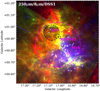 |
Fig. 1 Three-color composite image of M 16 using Herschel 250 μm (red), Spitzer-IRAC 8 μm (green), and DSS1-red (blue). The white circles indicate the positions of O and B stars (Evans et al. 2005). The pink and black dashed circles mark the 250 μm ring-like structure (M 16 H II region), and bubbles N19 and RCW165, respectively. |
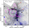 |
Fig. 2 90 cm emission (blue contours) superimposed on the Spitzer-IRAC 8 μm emission (grayscale). The pink dashed circles represent bubbles N19 and RCW165. The contour levels start from 0.021 Jy beam−1 (3σ) in steps of 3σ. The pink dashed lines indicate the dark IR clouds (Peretto & Fuller 2009), while the red arrows show two gas flows. The pink stars mark the positions of the two ionizing stars of N19 (Evans et al. 2005). |
3.2 Carbon monoxide molecular emission
The dust continuum emission only gives the distribution of the projected 2D gas around the M 16 H II region. To investigate in detail the gas structure associated with the M 16 H II region, we use 12CO J = 1−0, 13CO J = 1−0, and C18O J = 1−0 lines to trace the molecular gas. Figure 3 shows the averaged spectra of 12CO J = 1−0, 13CO J = 1−0, and C18O J = 1−0 over the entire M 16 H II region. All the 12CO J = 1−0, 13CO J = 1−0, and C18O J = 1−0 spectra show three peaks whose position is at 20.0 ± 0.4, 22.5 ± 0.4, and 25.0 ± 0.4 km s−1, which probably indicate different molecular components along the line of sight. Because the three components in the 12CO J = 1−0 and 13CO J = 1−0 spectra are too close, we are not able to see their distinct peaks, except for a few protrusions. The most obvious result is that the C18O J = 1−0 spectrum shows three clear peaks. Using the 12CO J = 1−0 data with an angular resolution of 180′′, Nishimura et al. (2017) also found three velocity components peaked at 19.5, 23.0, and 25.0 km s−1 through a latitude-velocity diagram for the M 16 region. Within the error range, our measured peak velocities for the three components are equal to those obtained by Nishimura et al. (2017). Compared with the 13CO J = 1−0 and C18O J = 1−0 spectral profiles, the optically thick 12CO line shows that there are two other velocity components, whose peak velocities are at 1.5 and 40.0 km s−1, respectively. These two velocity components may be related to background Galactic weak gas emission. Hence, the 13CO line is more suited to trace relatively dense gas. Using channel maps of the 13CO line, we further check the gas components which are associated with the M 16 H II region.
Figure 4 shows the 13CO J = 1−0 channel maps overlaid on the 8 μm emission, whose velocity ranges from 16 to 28 km s−1 in steps of 1 km s−1. Based on the morphology of the molecular gas associated with the previous identified bubble/ H II regions, pillars, and filaments, we find three velocity components. Component 1, which is located in velocity ranges from 16 to 24 km s−1, is mainly consistent with N19 and a massive gas clump identified in our data. The clump is situated in the northwest region of M 16. Component 2, observed from 20 to 24 km s−1, is associated with some pillars. Component 3, which is located in the velocity ranges from 23 to 28 km s−1, is mainly consistent with the NS filament. We suggest that these three components overlap and are connected to each other in velocity and space. To show the gas structure associated with each velocity component, we use the smaller integrated-velocity ranges to make the integrated-intensity images of 13CO J = 1−0. The three emissions are shown in Figs. 5a–c, overlaid on the 8 μm emission. The integrated-velocity ranges are shown on top of each map. The 13CO J = 1−0 emission of component 1 exhibits a small ring-like shape with an opening at the southwest, which just surrounds bubble N19. In addition, from component 1 to component 3, we find that some 13CO J = 1−0 emission with pillars is distributed around M 16, and the other emission towards the interior of the M 16 H II region. In component 3, we find two gas flows marked with red arrows, which are also seen in Fig. 2. Figures 5d–f show the C18O integrated-intensity images of the different velocity components overlaid with the 870 μm (red contours) and 8 μm emission (gray). The spatial distribution of the C18O J = 1−0 emission is similar to that of the 870 μm dust emission. The 870 μm emission also displays the NS filament.
Additionally, to construct a large-scale CO picture for the M 16 H II region, we also use the GRS 13CO J = 1−0 data. Figure 6 shows the13CO J = 1−0 integrated-intensity maps overlaid on the Herschel 250 μm emission. Each velocity component coincides well with its counterpart in the 250 μm emission. Both
emissions show a filamentary structure (large-scale filament). The G17.037+0.320 HII region (Anderson et al. 2014) is shown in Fig. 6. This expansion of the H II region might have divided the large-scale filament into two parts.
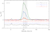 |
Fig. 3 Averaged spectra of 12CO J = 1− 0, 13CO J = 1− 0, and C18O J = 1− 0 over the entire M 16. We note that the intensities of 13CO J = 1− 0, and C18O J = 1− 0 are multiplied by a factor of 2 and 5 for clarity, respectively. The green lines represent the Gaussian fitted lines, with the resulting residuals shown below. The black vertical dashed lines mark the different velocity components. |
 |
Fig. 4 13CO J = 1− 0 channel maps from the integrated emission in step of 1 km s−1 overlaid on the Spitzer-IRAC 8 μm emission (gray). Central velocities are indicated in each image. The green arrows represent the pillars. |
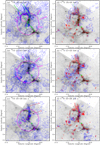 |
Fig. 5 Panels a–c: 13CO integrated intensity maps (blue contours) superimposed on the Spitzer-IRAC 8 μm emission (gray). The integrated-velocity ranges are shown on top of each image. The pink arrows mark the pillars, while the red dashed arrows indicate two gas flows. The blue contour levels start from 0.2 K km s−1(5σ) in a step of 1.6 K km s−1. The pink dashed circles represent M 16, N19, and RCW165. The green star marks the NGC 6611 cluster ionizing M 16. Panels d–f: C18O integrated intensity images overlaid with the ATLASGAL 870 μm (red contours) and 8 μm emission (gray). The blue contour levels start from 0.15 K km s−1(5σ) in a step of 0.75 K km s−1, while the redcontour levels start from 0.06 Jy beam−1 (3σ) in a step of 0.3 Jy beam−1. The green dashed lines mark the directions of position–velocity diagrams in Fig. 10. |
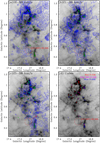 |
Fig. 6 Panels a–c: the 13CO J = 1− 0 emission in blue contours overlaid on the Herschel 250 μm emission in grayscale. The integrated-velocity ranges are shown on top of each image. The green circles represent the 870 μm dust cores, while the red dashed circle shows the position and size of G17.037+0.320 H II region from Anderson et al. (2014). The red arrow may present the shock direction. The two white dashed boxes indicate the compact region with six dust cores. Panel d: the ellipses also mark the positions, sizes, and position angles of the 870 μm dust cores, which are given in Table 1. The different colors mark the cores with different temperatures (T). If T > 24 K, the cores are marked in red, for 10 K < T < 24 K and T < 10 K in pinkand blue, respectively. |
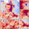 |
Fig. 7 870 μm emission (blue contours) superimposed on the Spitzer-IRAC 8 μm emission (red). The typical pillars and compact cores also are shown in the zoomed image. The white dashed circle outlines the M 16 H II region. The blue contour levels start from 0.06 Jy beam−1 (3σ) in steps of 0.3 Jy beam−1. |
3.3 The selected cores
Using the ATLASGAL catalog (Csengeri et al. 2014), we extract 51 dust cores in the large-scale filament. These cores are mainly distributed along the large-scale filament in Fig. 6, but more cores are located on the northern part of the large-scale filament. Since the 870 μm emission traces the distribution of dense cold dust, the northern part is likely to be the densest in the large-scale filament, which is associatedwith the M 16 H II region. We also present a zoomed image for the northern part of the large-scale filament to show the relation between M 16 and these cores, as shown in Fig. 7. There is a large compact clump located at the northwest ofM 16. We extracted six dust cores in the large clump from the catalog of Csengeri et al. (2014). Particularly, there are some cores that are situated in the heads of the pillars. Figure 7 also shows four typical pillars associated with the 870 μm cores. The parameters of the selected cores are listed in Table 1.
3.3.1 Excitation temperature, optical depth, and velocity dispersion
The CO molecular gas associated with M 16 has three different velocity components. The dust cores only show the 2D projected structure. We therefore need to determine to which component each core is linked. Within the effective radius of each core, we search for 12CO J = 1−0, 13CO J = 1−0, and C18O J = 1−0 spectra thatare located at or near the peak positions of the cores. We use three-velocity Gaussian components to fit the spectra. Considering whether the peak position of each core is associated with those of 13CO J = 1−0 and/or C18O J = 1−0 emissions, we lastly select a fitted component as the spectral parameters of the core. Compared with other components, we found that the strongest CO components are often associated with the cores. For part of the cores for which PMO CO data is not available, we use GRS 13CO J = 1−0 and JCMT 12CO J = 1−0 survey data to obtain the parameters. The fitted parameters are listed in Table 2, including brightness temperature (Tmb), FWHMspec, and centroid velocity (VLSR). For some cores, we cannot give the effective spectral value because of the weak signal (≤ 3σ). Since the cores are spatially unresolved by the CO data, the spectra used for each core also cover the surrounding matter. Hence, the fitted parameters may be underestimated for each core.
As 12CO emission is considered to be opticalthick, we use 12CO to calculate Tex via following the equation (Garden et al. 1991)
![\begin{equation*} {T_{\textrm{ex}}}=\frac{5.53}{{\textrm{ln}[1+5.53/(T_{\textrm{mb}}+0.82)]}}, \vspace*{-1pt}\end{equation*}](/articles/aa/full_html/2019/07/aa35024-19/aa35024-19-eq1.png) (1)
(1)
where Tmb is the corrected main-beam brightness temperature of 12CO. The derivedexcitation temperature in these cores ranges from 9.0 to 37.8 K with a mean value of 22.5 K. Figure 6d shows the positional distribution of the cores with different temperatures. The cores with temperature >20 K are mainly located in the northern part of the large-scale filament, which is interacting with the M 16 H II region. In addition, we assume that the excitation temperatures of 12CO and 13CO have the same values in both cores. The optical depth (τ) can be obtained by the following equation (Garden et al. 1991)
![\begin{equation*} {\tau(^{13}\textrm{CO})}=-\textrm{ln}\left[1-\frac{T_{\textrm{mb}}}{5.29/[\textrm{exp}(5.29/T_{\textrm{ex}}) -1]-0.89}\right]. \vspace*{-1pt}\end{equation*}](/articles/aa/full_html/2019/07/aa35024-19/aa35024-19-eq2.png) (2)
(2)
The derived optical depth is 0.2–1.9 with a median value of 0.5, indicating that the 13CO emission is optically thin in most of the cores. Hence, we use the 13CO VLSR to determine the distance of each core. The distances to the cores are estimated using the Bayesian Distance Calculator 4 (Reid et al. 2016). We obtain that the distance of these cores is about 1.85 ± 0.2 kpc. The distance to NGC 6611 is estimated to be in the range 1.75–2.00 kpc (Hillenbrand et al. 1993; Loktin & Beshenov 2003; Guarcello et al. 2007; Wolff et al. 2007; Gvaramadze & Bomans 2008). M 16 is excited by numerous O and B stars within the open cluster NGC 6611. By comparing the distances obtained for the cores, we demonstrate that the cores are associated with the M 16 H II region.
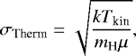
The 1D thermal velocity dispersion in each core, συ, is determined by
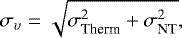 (3)
(3)
where σTherm and σNT are the thermal and nonthermal 1D velocity dispersions. For all the cores, σNT and σTherm can be obtained using, respectively,
![\begin{equation*} {\sigma_{\textrm{NT}}}=\left[\sigma_{\textrm{C}^{18}\textrm{O}}^{2}-\frac{kT_{\textrm{kin}}}{m_{\textrm{C}^{18}\textrm{O}}\mu}\right]^{1/2} ,\end{equation*}](/articles/aa/full_html/2019/07/aa35024-19/aa35024-19-eq4.png) (4)
(4)
 (5)
(5)
where Tkin is the kinetic temperature in the core. If the densities of the cores are high enough so that LTE conditions hold, Tex can be adopted as Tkin (Fehér et al. 2017). For the dense ATLASGAL cores, here we take Tex as Tkin. Further, μ = 2.72 is the mean atomic weight, mH is the mass of an H atom,  = (
= ( ) is the 1D velocity dispersion of C18O J = 1−0, and
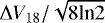
  is the mass of C18O J = 1−0. For the 51 cores, only 35 cores have C18O J = 1−0 emission above 3σ. Their derived parameters are summarized in Table 3. The mean thermal 1D velocity dispersion of these cores ranges from 0.22 to 0.33 km s−1 with a mean value of 0.27 km s−1. The nonthermal 1D velocity dispersion of these cores ranges from 0.34 to 1.34 km s−1 with a mean value of 0.84 km s−1. The mean 1D velocity dispersion συ ranges from 0.52 to 1.36 km s−1 with a mean value of 0.87 km s−1. Figure 8 shows the distributions of excitation temperature, optical depth, and velocity dispersion; we obtain that the nonthermal motion is dominating for the velocity dispersion.
Parameters of the selected dust cores (Csengeri et al. 2014).
3.3.2 Mass, size, and volume density
We use the 870 μm flux of the cores to estimate their mass. Assuming optically thin emission, the mass is given by (Hildebrand 1983)
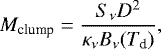 (6)
(6)
where Sν and D correspond to the flux density at the frequency ν and the distance to the cores. The ratio of gas to dust was adopted as 100 (Schuller et al. 2009), κν is the dust opacity, which is adopted as 0.01 cm2 g−1 at 870 μm (Ossenkopf & Henning 1994), and Bv(Td) is the Planck function for the dust temperature Td and frequency ν. The gas and dust temperatures are coupled if the gas densities are higher than 2 × 104 cm−3 (Goldsmith 2001; Galli et al. 2002). Csengeri et al. (2014) obtained that the mean gas density of the ATLASGAL clumps associated with GMCs is ~3 × 105 cm−3. Hence, we take the excitation temperature as a dust temperature to estimate the mass of these cores.
Assuming that the cores have roughly spherical shapes, the average volume density of each core was calculated as
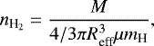 (7)
(7)
where Reff is the effective radius of each core, which is determined by
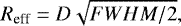 (8)
(8)
where FWHM is the deconvolved size of the cores, respectively. The obtained Reff are listed in Col. 3 of Table 3. Core radius ranges from 0.09 to 0.25 pc. The masses of these cores range from 11.9 ± 1.8 to 357.3 ± 53.6 M⊙ with a total mass of 2716 M⊙, while the average volume density ranges from 2.5 × 10⁴ to 5.9 × 105 cm−3. The typical uncertainties of the parameters largely originate from the uncertainties in flux estimation. The final flux uncertainty for the compact cores should be lower than 15% (Schuller et al. 2009), which can propagate to other parameters.
3.4 Young stellar objects associated with the larger filament
Since the Spitzer-IRAC bands are highly sensitive to the emission from the circumstellar disks and envelopes, the IRAC color–color diagrams are used to identify young stellar objects (YSOs) with infrared excess in star-formingregions and categorizing them according to evolutionary stages (Allen et al. 2004). In order to study the YSO population within the large-scale filament, we use the GLIMPSE I Spring’07 catalog to search for YSOs. Based on the criteria of Allen et al. (2004), we selected near-infrared sources with 3.6, 4.5, 5.8, and 8.0 μm detections from the catalogue. All selected sources have photometric uncertainties <0.2 mag in all four IRAC bands. In the large-scale filament associated with the M 16 H II region, we found 267 Class I YSOs and 886 Class II YSOs. Class I YSOs are protostars with circumstellar envelopes and a timescale of the order of ~ 105 yr, while Class II YSOs are disk-dominated objects with a ~106 yr (André & Montmerle 1994). The Class III YSOs are the pre-main sequence stars. Figure 9shows the spatial distribution of these Class I and Class II YSOs. To investigate the positional relation of YSOs with the large-scale filament, we also overlaid the selected Class I and Class II YSOs on the 13CO J = 1 − 0 emission (contours) and 250 μm emission (gray scale). Here the integrated-velocity range (16–24 km s−1) of 13CO J = 1 − 0 covers all the components. Class I sources in Fig. 9a are found to be mostly concentrated in two regions, which are marked by two white dashed circles. One region is associated with the NGC 6611 cluster responsible for the ionization of M 16, the other region is situated at the edge of M 16. Although most of the Class II YSOs in Fig. 9b appear to be dispersedly distributed across the selected region, there are still some Class II YSOs concentrated in the position of the NGC 6611 cluster. Since the whole region has many Class III YSOs, we do not show the distribution of these YSOs in Fig. 9 to avoid confusion.
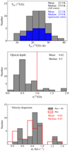 |
Fig. 8 Distributions of excitation temperature, optical depth, and velocity dispersion for the selected cores. |
Fitted parameters of 12CO J = 1− 0, 13CO J = 1− 0, and C18O J = 1− 0 spectra for the selected cores.
Calculated parameters of the selected dust cores.
4 Discussion
4.1 Gas structure associated with M 16
The CO molecular gas and cool dust emissions are mainly located in the northeastern part of the M 16 H II region. The expansion of M 16 is likely to be blocked by the molecular gas along this direction. The western CO and dust emission of M 16 are very weak, allowing the expansion of M 16 to break the molecular gas and create a cavity. On large scale, the 13CO J = 1−0 emission consists of three velocity components. Each component shows a filamentary structure extended along the north-south direction. The spatial overlap of these three components along the line of sight suggests that the large-scale filament has three layers. From component 1 to component 3, we find that several pillars, revealed by their 13CO J = 1−0 emission, are distributed over the edges of the entire M 16 region. The northeastern part of the large-scale filament may be disrupted into some small IRDCs because of the expansion of the M 16 H II region, which is similar to the case of the filamentary IRDC G34.43+0.24 (Xu et al. 2016). The presence of several smaller IRDCs and pillars suggests that M 16 is interacting with the large-scale filament and has reshaped its structure. Both the large-scale filament associated with M 16 and the filamentary IRDC G34.43+0.24 show the 8 μm IR dark and bright parts. The bright parts of the IRDC are associated with H II regions and IR bubbles. Hence, the associated H II regions may illuminate the dark parts of the large-scale filament.
Moreover, to investigate the dynamic structure of the molecular gas surrounding the N19 bubble, we made a position–velocity (PV) diagram along the northwestern direction towards the NGC 6611 cluster. The cutting direction goes through N19. In Fig. 10a, the two red vertical lines mark the edges of N19. The diameter of the bubble is obtained from Fig. 5. The green arrows are assumed to indicate the direction of the shock from the M 16 H II region, while the blue dashed line marks the compressed surface of the molecular cloud. From Fig. 10a, we can see that the M 16 H II region is probably interacting with three molecular layers. Furthermore, we also observe the CO emission that peaks at 16 km s−1 towards N19, which is likely to be the front or back side of the bubble if the bubble is a sphere. A molecular pillar marked by a blue arrow at the edge of N19 might have been created by the expansion of N19. In Fig. 5, the 870 μm emission delineates the NS filament. To explore the structure of this NS filament, we use two directions to make the PV diagram along the NS filament constructed from the 13CO J = 1−0 emission. These directions are shown in Fig. 5. As seen in Fig. 10, the northern part of the NS filament shows a single component, suggesting a single coherent object which is associated with component 1 in velocity. The remaining part contains three different velocity components. Hence, we conclude that the whole NS filament seen in the Herschel data and on the ATLASGAL 870 μm emission is the projection effect from the molecular gas of the different velocity components.
 |
Fig. 9 13CO J = 1− 0 emission (blue contours) and 870 μm emission (red contours) superimposed on the Herschel 250 μm emission in grayscale. The green circles represent the identified class I and II YSOs. The white circles outline the regions of YSO accumulation. Panel a: distribution of the Class I YSOs. Panel b: distribution of Class II YSOs. |
4.2 Cores properties
In the large-scale filament, we found 51 dust cores. The excitation temperatures in these cores range from 9.0 to 37.8 K with a mean value of 22.5 K. Generally, dust is heated by UV and IR emission, while gas is heated only by UV through photo-electric heating (Hollenbach & Tielens 1997). Previous observations indicated that cold dark cores may have a typical excitation temperature of ~10.0 K (Du & Yang 2008; Meng et al. 2013; Liu et al. 2014). Compared to the cold dark cores, the dust cores in the large-scale filament are likely to be heatedby the UV emission from the M 16 H II region. Guzmán et al. (2015) studied about 3000 molecular clumps from ATLASGAL data at 870 μm. They obtained a mean dust temperature of 16.8 K for the quiescent clumps, 18.6 K for protostellar clumps, and 23.7 K and 28.1 K for clumps associated with H II and PDR, respectively. Through visual inspection of Spitzer images at 3.6, 4.5, 8.0, and 24 μm, Foster et al. (2011) developed a criterion for classification of core evolution. Specifically, cores which are dark at GLIMPSE wavelengths (3.6-8 μm) are identified as quiescent, cores with a MIPSGAL 24 μm point source are identified as protostellar, and cores with extended 8 μm flux are identified as H II regions. Based on the criterion of Foster et al. (2011), we classify the 51 cores in the large-scale filament into three evolutionary stages. Column 12 in Table 3 gives the classification of the cores, as quiescent (20 cores), protostellar (3 cores), H II/PDR (28 cores). Because some cores are distributed close to the M 16 H II region, the H II/PDR classification carries significant uncertainty. The excitation temperatures of the 20 identified quiescent cores in the large-scale filament range from 14.2 to 30.8 K with a mean value of 22.2 K. Some of the quiescent cores are also called IR dark cores in Guzmán et al. (2015). Assuming that dust and gas temperatures are similar (see Sect. 3.3.2), the mean value (22.2 K) of the temperature for quiescent cores in the large-scale filament is higher than that (16.8 K) of Guzmán et al. (2015), suggesting that the cores in the large-scale filament are heated by the radiation of the M 16 H II region, not by an internal heating due to sources in the cores. At a temperature < 20 K, the molecular gas is cold (Guzmán et al. 2015; Egan et al. 1998; Carey et al. 1998). In the large-scale filament, there are 34 cores whose excitation temperature is higher than 20.0 K, meaning that at least 67% of the cores have been heated. From Fig. 6d, we also see that the majority of the heated cores is spatially close to the M 16 HII region.
To determine whether these cores have sufficient mass to form massive stars, we can use the mass–size relation given by Kauffmann & Pillai (2010). The radii of the cores range from 0.09 to 0.25 pc, while the masses range from 12 to 357 M⊙. Figure 11 presents a mass-versus-radius plot for all the cores. The surface density of 0.024 g cm−2 gives the average surface density thresholds for efficient star formation. The thresholds, shown as green lines in Fig. 11, are derived by Lada et al. (2010) and Heiderman et al. (2010), respectively. As can be seen from Fig. 11, 51 cores (100%) are located above the lower surface density limit of 0.024 g cm−2. Krumholz & McKee (2008) suggested that the cores with a mass surface density of >1 g cm−2 can avoid further fragmentation and form massive stars. Moreover, Kauffmann & Pillai (2010) investigatedthe mass–radius relationship of cores and found the empirical relationship 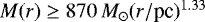 as the threshold to determine whether cores can potentially form massive stars. We note that when deriving their relationship, Kauffmann & Pillai (2010) reduced the dust opacities of Ossenkopf & Henning (1994) by a factor of 1.5. Because this correction has not been applied here, we have rescaled the relationship
 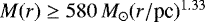 , which is also given by Urquhart et al. (2013). We find that about 45% of all the identified cores are above the rescaled threshold, indicating that these cores are dense and massive enough to potentially form massive stars. In the bubble-shaped nebula Gum 31, 37% of the 870 μm clumps lie in or above the massive-star formation threshold (Duronea et al. 2015). We suggest that HII regions can help in creating a larger number of massive clumps and cores, but more examples are needed to make a firm conclusion.
 |
Fig. 10 Panel a: position–velocity diagram of the 13CO J = 1− 0 emission along the northwest of the N19 bubble (see the green dashed lines in Fig. 5a panel). The red dashed lines mark the edges of the N19 bubble. The green arrows show the direction of the interaction between the HII region of M 16 and the molecular gas. The blue arrow shows the high-velocity gas, whileblue dashed lines indicate the compressed positions. Panel b: position–velocity diagram of the 13CO J = 1− 0 emission along the NS filament (see the green dashed lines in Fig. 5 a panel). The blue dashed lines shows the three velocity components, which are mentioned in Sect. 3.2. We refer to the discussion about the PV diagrams in Sect. 4.1 |
 |
Fig. 11 Mass–radius distributions for the ATLASGAL 870 μm cores. The green dots show the six cores in the small filament, while the red dots show the six cores in the large clump. The surface density of 0.024 g cm−2 shown in green lines gives the average surface density thresholds for efficient star formation, which are derived by Lada et al. (2010) and Heiderman et al. (2010), respectively. A core with a mass surface density of >1 g cm−2 (shown as a green line) can avoid further fragmentation and form massive stars (Krumholz & McKee 2008). We refer to the discussion about the lines in the Sect. 4.2. |
4.3 Core formation
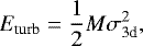
In a filament, core formation may be regulated by the interplay between gravity, turbulence, and magnetic field (Li et al. 2015). Several pillars are found in the large-scale filament associated with M 16. Particularly, there are some cores that are situated in the heads of the pillars. With the expansion of an H II region, Schneider et al. (2012) suggested that when the ionized gas pressure dominates the ram pressure of the initial turbulence in the molecular cloud, this leads to the formation of the cores and pillars. This is a strong indication that the pillars in M 16 are produced by the interplay of pre-existing turbulent structures and ionizing radiation (Gritschneder et al. 2010). Here at least 67% of the cores in the large-scale filament have been heated by the M 16 H II region. However, compared with the thermal motion, we suggest thatthe nonthermal motion may dominate the velocity dispersion in the cores of the large-scale filament. The nonthermal motions in the cores are generally interpreted as being due to supersonic turbulence (e.g., Zuckerman & Evans 1974; McKee & Ostriker 2007), which is responsible for the core formation in the large-scale filament. Using C18O J = 1−0, the nonthermal 1D velocity dispersion σNT is 0.27 km s−1 for the Taurus molecular cloud (TMC), and 0.35 km s−1 for the California molecular cloud (CMC) (Meng et al. 2013). The TMC is a typical site of low-mass star formation. The CMC is in an early state of evolution and has not achieved the internal physical conditions to promote more active star formation (Lada et al. 2009). Hence, both TMC and CMC have less star-forming activity compared to M 16. The mean σNT of these cores is 0.84 km s−1 for C18O J = 1−0 in the large-scale filament associated with the M 16 H II region. Compared with the TMC and CMC, the higher σNT in the large-scale filament may be created by the feedback from the M 16 H II region. As the pillars are seen adjacent to M 16, the H II region may give rise to the strong turbulence in the large-scale filament.
In molecular clouds, turbulence has been shown to dissipate quickly (Stone et al. 1998; Mac Low 1999; Orkisz et al. 2017) if the external driving is stopped, resulting in the need to continuously drive turbulence via stellar feedback (Ostriker et al. 2010; Offner & Liu 2018). Here we can estimate the turbulent energy of the large-scale filament, which is given by
 (9)
(9)
where 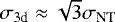 , which is the 3D turbulent velocity dispersion. In the large-scale filament, we found the mean σNT to be 0.84 km s−1, which is obtained from Sect. 3.3. The mass of the filament can be obtained by
 (10)
(10)
where  is the column density, and S is the area of the large-scale filament, which can be determined by the Herschel 250 μm data in Fig. 6. Using the Herschel data and spectral energy distribution (SED) fitting, Hill et al. (2012) obtained that the column density of the dense large-scale filament associated with M 16 is (3–7) × 1022 cm−2. We derive a mass of (4.3–9.9) × 105 M⊙ for the large-scale filament and estimate the turbulent energy of the large-scale filament to be about (1.8–4.2) × 1049 erg. The formation of the M 16 shell may be attributed to the expansion of the M 16 H II region that is ionized by a few O and B stars. Sofue et al. (1986) obtained that the total kinetic energy ejected from these O and B stars is evaluated as about 7 × 1050 erg, which is one order of magnitude higher than the obtained turbulent energy in the large-scale filament. For an H II region, Freyer et al. (2003) and Xu et al. (2018) indicated that the ionization energy is one order of magnitude higher than the kinetic energy and thermal energy. Hence, the energies from the M 16 H II region can help to maintain the strong turbulence in the large-scale filament via energy injection.
 |
Fig. 12 870 μm emission (blue contours) superimposed on the 8 μm emission (gray). The two regions are as also shown in the two white dashed boxes in Fig. 6. The blue contour levels start from 3σ (0.15 Jy beam−1) and rise in steps of 2σ. The green ellipses represent the 870 μm cores. The red stars mark the positions of the MSX6C G016.9270+00.9599 and MSX6C G016.9261+00.2854 H II regions (Urquhart et al. 2011). The red squares indicate IRAS sources, while the red triangle shows the water maser (Braz & Epchtein 1983). The ATLASGAL beam (19′′) is shown as the green filled circle in the bottom right-hand corner. |
4.4 Turbulent fragmentation
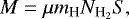
In the large-scale filament, there are six different compact cores in a large clump and in a small filament (southern filament), as shown in Figs. 12a and b, respectively. The large clump is associated with the dark IR cloud SDC G16.955+0.960, while the southern filament is consistent with SDC G16.925+0.279 (Peretto & Fuller 2009). Because both the clump and filament are also associated with an H II region (Urquhart et al. 2011) and an IRAS source, they are massive star-forming regions. In the large clump, the mean excitation temperature and σv of the six cores are 19.9 K and 0.93 km s−1, respectively. Adopting the mean excitation temperature as the dust temperature (see Sect. 3.3.2), we obtained a mass of 2569 M⊙ for the large clump. Figure 11 shows that five of the six cores (red dots) in the large clump are dense and massive enough to potentially form massive stars. Particularly, the mass surface density of core 14 is higher than 1 g cm−2. According to Krumholz & McKee (2008), this means that because of the prevention through radiative feedback, this core will not further fragment into low-mass cores, thus allowing high-mass star formation. Moreover, core 14 is also associated with the MSX6C G016.9270+00.9599 H II region in space (Urquhart et al. 2011), as shown in Fig. 12a, therefore further supporting the results of Krumholz & McKee (2008). Assuming that the clump is governed by Jeans instability, we estimate the Jeans mass, which is given as  (Wang et al. 2014). From Eq. (7), we derive the number density n = 9450 cm −3. Taking the mean excitation temperature (19.9 K) of the six cores as that of the clump, we determine MJ ~ 8.0 M⊙. The masses of the six cores in the clump range from 19 to 357 M⊙, which is larger than the Jeans mass (8.0 M⊙), indicating that these cores may have formed in the clump through the turbulent core model (McKee & Tan 2002).
For the southern filament, the mean excitation temperature of the six cores is 19.9 K, which is the same as that in the clump. From Fig. 11, we see that only one core is massive enough to form massive stars in the southern filament, which is different from that in the clump. If the turbulence dominates in the southern filament, the critical linear mass density can be estimated as  = 84
= 84 M⊙ pc−1 (Jackson et al. 2010), where ΔV is the linear width in units of km s−1. We did not observe the southern filament in C18O. The mean ΔV of 13CO in the southern filament is 2.4 km s−1, while the mean C18O ΔV of the large-scale filament is also 2.4 km s−1. Adopting a mean ΔV of 2.4 km s−1 for the southern filament, we obtain
 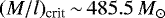 pc−1. From Fig. 12, we measure the length of the southern filament to be 5.6 pc. Using Eq. (6), the derived mass of the southern filament is 1613 M⊙. Using the mass and length, we derive a linear mass density of M∕l = 289.6 M⊙ pc−1, which is roughly consistent with (M∕l)crit. Considering the uncertainties of the FWHM, the turbulent motion may help to stabilize the southern filament against radial collapse (Jackson et al. 2010; Beuther et al. 2015).
In addition, we can calculate a core formation efficiency (CFE) for the compact clump and the southern filament, which is given by Mcore/Mclump. The total mass of the cores in the clump is 552 ± 26 M⊙, while this is 260 ± 8 M⊙ in the southern filament. We obtain that the CFE for the clump is 22 ± 3%, while this value is 16 ± 2% in the southern filament. The southern filament is likely to be compressed by the G17.037+0.320 H II region (Anderson et al. 2014), as shown in Fig. 6. Compared with the southern filament, the clump is closer to the M 16 H II region. The strong feedback from M 16 may create the higher CFE. The CFE in the GMC of the Milky Way is about 11.0% (Battisti & Heyer 2014). In the W3 GMC, the CFE in the filament compressed by the H II region is in the range 26–37%, while this value is 5–13% in the diffuse region (Moore et al. 2007). Eden et al. (2013) also gave a CFE in the region associated with H II regions of about 40%. The obtained clump formation efficiency in the filament G47.06+0.26 associated with bubbles/H II regions is ~15% (Xu et al. 2018). From the above analysis, we conclude that the molecular clouds associated with H II regions have a higher CFE. The higher CFE may be created by the ionization feedback from the H II regions.
4.5 The NGC6611 cluster and YSO formation
We have shown that the M 16 H II region interacts with a large-scale filament with three layers. M 16 is ionized by numerous O and B stars within the open cluster NGC 6611. Because the large-scale filament is associated with some IRDCs, as shown in the pink dashed lines in Fig. 2, the NGC 6611 cluster may form in a dark IR filament. The age of the YSOs in NGC 6611 is estimated to be 0.25–3 Myr (Hillenbrand et al. 1993). We also use the Spitzer-IRAC data to identify Class I and Class II YSOs. Class I YSOs have an age of ~ 105 yr, while this is ~106 yr for Class II YSOs (André & Montmerle 1994). The selected YSOs (Class I and Class II) are also concentrated in NGC 6611. Furthermore, Hillenbrand et al. (1993) found that the stars of 3 M⊙ < mass < 8 M⊙ have ages ranging from 0.25 to at least 1 Myr, while the mean age of the stars with a mass of >9 M⊙ is 2 ± 1 Myr. The stars with the ages from 0.25 to 1 Myr may belong to Class I and Class II YSOs. From the ages and masses of the cluster NGC 6611 members, the massive stars may form before low-mass stars in a cluster.
Additionally, a high density of Class I YSOs is also found to be located at the edges of the M 16 H II region. Since some of the selected Class I and Class II YSOs are clustered, it is unlikely that they are all simply foreground and background stars. It is more likely that most of the clustered Class I and Class II YSOs are physically associated with the large-scale filament. Through the Hertzprung-Russell (HR) diagram, Hillenbrand et al. (1993) obtained that the age of NGC 6611 is likely to be about 2 ± 1 Myr. Because M 16 is excited by the O and B stars within the open cluster NGC 6611, we assume that the dynamical age of M 16 is the same as that of NGC 6611. Comparing the dynamical age of the M 16 H II region with those of the Class I YSOs, we conclude that the formation of these Class I YSOs might have been triggered by the H II region M 16. Moreover, the IR bubble N19 and RCW165 are located in the dense region of the large-scale filament, and interact with the filament. The ionized stars of N19 and RCW165 may be second-generation massive stars, whose formation was triggered by the expansion of the M 16 H II region.
5 Conclusions
Using the PMO molecular 12CO J = 1−0, 13CO J = 1−0, and C18O J = 1−0 data combined with IR and radio archival data, we present a comprehensive large-scale picture of the gas and dust towards the M 16 H II region. The main findings are summarized as follows.
- 1.
The H II region M 16 shows an irregular ionized-gas cavity, which is enclosed by the cool dust traced by the 250 μm emission, and PAH emission traced by the 8 μm emission. From CO data, we observe a large-scale filament with three main velocity components, whose peak velocities are 20.0, 22.5, and 25.0 km s−1. These three components overlap with each other, both in velocity and space, suggesting that the large-scale is made of three layers.Because the large-scale filament is associated with some IRDCs, the NGC 6611 cluster may have formed in a dark IR filament. The presence of pillars associated with each velocity component indicates that the M 16 H II region is interacting with the large-scale filament and has reshaped the structure of the surrounding gas.
- 2.
In the whole large-scale filament, we find 51 dust cores from the ATLASGAL catalog and classify the cores into three evolutionarystages, as quiescent (20 cores), protostellar (3 cores), and H II/PDR (28 cores). We find that 45% of all the identified cores are dense and massive enough to potentially form massive stars. The excitation temperature in these cores of the filament range from 9.0 to 37.8 K with a mean value of 22.5 K. The mean excitation temperature of the identified quiescent cores is 22.2 K. The mean temperature for the quiescent cores suggests that the cores are externally heated by the M 16 H II region and not internally due to sources in the cores. If the temperature of the heated cores is >20 K, here at least 67% of the cores have been heated. The majority of the heated cores is spatially close to the M 16 H II region.
- 3.
Compared with the thermal motion, the turbulence created by the nonthermal motion leads to the formation of the cores. Compared with the TMC and CMC, the higher nonthermal velocity dispersions in the large-scale filament may be created by the M 16 H II region. Compared with the large-scale turbulent energy (1.8–4.2 × 1049 erg), the energies of the M 16 H II region can help to maintain the strong turbulence by injecting energy. A large clump and a southern filament contain six compact cores. The clump and the filament have been formed through the gas turbulence.
- 4.
In the large-scale filament, we find that the CFE for the clump is 22 ± 3%, while this value is 16 ± 2% in the southern filament. The higher CFE may be created by feedback from the nearby H II regions.
- 5.
Comparing the dynamical age of the M 16 H II region with the Class I YSOs located at its edges, we suggest that the formation of these YSOs may have been triggered by the expansion of the M 16 H II region. The ionized stars of N19 and RCW165 may also be second-generation massive stars.
Acknowledgements
We thank the referee for insightful comments which improved the clarity of this manuscript. We thank the Key Laboratory for Radio Astronomy, CAS, for partly supporting the telescope operation. This work has made use of data from the Spitzer Space Telescope, which is operated by the Jet Propulsion Laboratory, California Institute of Technology under a contract with NASA. The ATLASGAL project is a collaboration between the Max-Planck-Gesellschaft, the European Southern Observatory (ESO) and the Universidad de Chile. This includes projects E-181.C-0885, E-078.F-9040(A), M-079.C-9501(A), M-081.C-9501(A) plus Chilean data. This work was supported by the National Natural Science Foundation of China (Grant Nos. 11673066, 11703040, and 11847309), the Youth Innovation Promotion Association of CAS, the young researcher grant of national astronomical observatories, Chinese academy of sciences, and also supported by the Open Project Program of the Key Laboratory of FAST, NAOC, Chinese Academy of Sciences. A.Z. thanks the support of the Institut Universitaire de France.
References
- Allen, L. E., Calvet, N., & D’Alessio, P. 2004, ApJS, 154, 363 [NASA ADS] [CrossRef] [Google Scholar]
- André, P., & Montmerle, T. 1994, ApJ, 420, 837 [NASA ADS] [CrossRef] [Google Scholar]
- Andersen, M., Knude, J., Reipurth, B., et al. 2004, A&A, 414, 969 [NASA ADS] [CrossRef] [EDP Sciences] [Google Scholar]
- Anderson, L. D., Zavagno, A., Deharveng, L., et al. 2012, A&A, 542, A10 [NASA ADS] [CrossRef] [EDP Sciences] [Google Scholar]
- Anderson, L. D., Bania, T. M., Balser, D. S., et al. 2014, ApJS, 212, 1 [NASA ADS] [CrossRef] [Google Scholar]
- Arce, H. G., Borkin, M. A., Goodman, A. A., Pineda, J. E., & Beaumont, C. N. 2011, ApJ, 742, 105 [NASA ADS] [CrossRef] [Google Scholar]
- Battisti, A. J.,& Heyer, M. H. 2014, ApJ, 780, 173 [NASA ADS] [CrossRef] [EDP Sciences] [Google Scholar]
- Benjamin, R. A., Churchwell, E., & Babler, B. L. 2003, PASP, 115, 953 [NASA ADS] [CrossRef] [Google Scholar]
- Beuther, H., Ragan, S. E., Johnston, K., et al. 2015, A&A, 584, A67 [NASA ADS] [CrossRef] [EDP Sciences] [Google Scholar]
- Braz, M. A., & Epchtein, N. 1983, A&AS, 54, 167 [NASA ADS] [Google Scholar]
- Brogan, C. L., Gelfand, J. D., Gaensler, B. M., et al. 2006, ApJ, 639, L25 [NASA ADS] [CrossRef] [Google Scholar]
- Carey, S. J., Clark, F. O., Egan, M. P., et al. 1998, ApJ, 508, 721 [NASA ADS] [CrossRef] [Google Scholar]
- Carey, S. J., Feldman, P. A., Redman, R. O., et al. 2000, ApJ, 543, L157 [NASA ADS] [CrossRef] [Google Scholar]
- Churchwell, E., Povich, M. S., Allen, D., et al. 2006, ApJ, 649, 759 [NASA ADS] [CrossRef] [Google Scholar]
- Csengeri, T., Urquhart, J. S., Schuller, F., et al. 2014, A&A, 565, A75 [NASA ADS] [CrossRef] [EDP Sciences] [Google Scholar]
- Csengeri, T., Bontemps, S., Wyrowski, F., et al. 2017, A&A, 601, A60 [NASA ADS] [CrossRef] [EDP Sciences] [Google Scholar]
- Deharveng, L., Lefloch, B., Zavagno, A., et al. 2003, A&A, 408, 25 [NASA ADS] [CrossRef] [EDP Sciences] [Google Scholar]
- Dewangan, L. K., & Ojha, D. K. 2013, MNRAS, 429, 1386 [NASA ADS] [CrossRef] [Google Scholar]
- Dewangan, L. K., Ojh, D. K., Luna, A., et al. 2016, ApJ, 819, 66 [NASA ADS] [CrossRef] [Google Scholar]
- Dewangan, L. K., Baug, T., Ojha, D. K., Zinchenko, I., & Luna, A. 2018, ApJ, 864, 54 [NASA ADS] [CrossRef] [Google Scholar]
- Du, F., & Yang, J. 2008, ApJ, 686, 384 [NASA ADS] [CrossRef] [Google Scholar]
- Dubout-Crillon, R. 1976, ApJ, 25, 25 [NASA ADS] [Google Scholar]
- Duronea, N. U., Vasquez, J., Gómez, L., et al. 2015, A&A, 682, A2 [NASA ADS] [CrossRef] [EDP Sciences] [Google Scholar]
- Eden, D. J., Moore, T. J. T., Morgan, L. K., Thompson, M. A., & Urquhart, J. S. 2013, MNRAS, 431, 1587 [NASA ADS] [CrossRef] [Google Scholar]
- Egan, M. P., Shipman, R. F., Price, S. D., et al. 1998, ApJ, 495, L199 [NASA ADS] [CrossRef] [Google Scholar]
- Elmegreen, B. G., & Lada, C. J. 1977, ApJ, 214, 725 [NASA ADS] [CrossRef] [Google Scholar]
- Evans, C. J., Smartt, S. J., Lee, J.-K., et al. 2005, A&A, 437, 467 [NASA ADS] [CrossRef] [EDP Sciences] [Google Scholar]
- Faimali, A., Thompson, M. A., Hindson, L., et al. 2012, MNRAS, 426, 402 [NASA ADS] [CrossRef] [Google Scholar]
- Fehér, O., Juvela, M., Lunttila, T., et al. 2017, A&A, 606, A102 [NASA ADS] [CrossRef] [EDP Sciences] [Google Scholar]
- Foster, J. B., Jackson, J. M., Barnes, P. J., et al. 2011, ApJS, 197, 25 [NASA ADS] [CrossRef] [Google Scholar]
- Freyer, T., Hensler, G., & Yorke, H. W. 2003, ApJ, 594, 888 [NASA ADS] [CrossRef] [Google Scholar]
- Galli, D., Walmsley, M., & Gonçalves, J. 2002, A&A, 394, 275 [NASA ADS] [CrossRef] [EDP Sciences] [Google Scholar]
- Garden, R. P., Hayashi, M., Hasegawa, T., et al. 1991, ApJ, 374, 540 [NASA ADS] [CrossRef] [Google Scholar]
- Geen, S., Soler, J. D., & Hennebelle, P. 2017, MNRAS, 471, 4844 [NASA ADS] [CrossRef] [Google Scholar]
- Goldsmith, P. F. 2001, ApJ, 557, 736 [NASA ADS] [CrossRef] [MathSciNet] [Google Scholar]
- Gritschneder, M., Burkert, A., Naab, T., & Walch, S. 2010, ApJ, 723, 971 [NASA ADS] [CrossRef] [Google Scholar]
- Guarcello, M. G., Prisinzano, L., Micela, G., et al. 2007, A&A, 462, 245 [NASA ADS] [CrossRef] [EDP Sciences] [Google Scholar]
- Guzmán, A. E., Sanhueza, P., Contreras, Y., et al. 2015, ApJ, 815, 130 [NASA ADS] [CrossRef] [Google Scholar]
- Gvaramadze, V. V., & Bomans, D. J. 2008, A&A, 490, 1071 [NASA ADS] [CrossRef] [EDP Sciences] [Google Scholar]
- Haid, S., Walch, S., Seifried, D., et al. 2018, MNRAS, 478, 4799 [NASA ADS] [CrossRef] [Google Scholar]
- Handa, T., Sofue, Y., Reich, W., et al. 1986, PASJ, 38, 347 [NASA ADS] [Google Scholar]
- Heiderman, A., Evans, II, N. J., Allen, L. E., Huard, T., & Heyer, M. 2010, ApJ, 723, 1019 [NASA ADS] [CrossRef] [Google Scholar]
- Hester, J. J., Scowen, P. A., Sankrit, R., et al. 1996, AJ, 111, 2349 [NASA ADS] [CrossRef] [Google Scholar]
- Hill, T., Motte, F., Didelon, P., et al. 2012, A&A, 542, A114 [NASA ADS] [CrossRef] [EDP Sciences] [Google Scholar]
- Hildebrand, R. H. 1983, QJRAS, 24, 267 [NASA ADS] [Google Scholar]
- Hillenbrand, L. A., Massey, P., Strom, S. E., & Merrill, K. M. 1993, AJ, 106, 1906 [NASA ADS] [CrossRef] [Google Scholar]
- Hollenbach, D. J., & Tielens, A. G. G. M. 1997, ARA&A, 35, 179 [NASA ADS] [CrossRef] [Google Scholar]
- Jackson, J. M., Rathborne, J. M., Shah, R. Y., et al. 2006, ApJS, 163, 145 [NASA ADS] [CrossRef] [Google Scholar]
- Jackson, J. M., Finn, S. C., Chambers, E. T., et al. 2010, ApJ, 719, L185 [NASA ADS] [CrossRef] [Google Scholar]
- Kauffmann, J., & Pillai, T. 2010, ApJ, 723, L7 [NASA ADS] [CrossRef] [Google Scholar]
- Kim, J.-G., Kim, W.-T., Ostriker, E. C., & Skinner, M. A. 2013, ApJ, 851, 93 [Google Scholar]
- Krumholz, M. R., & McKee, C. F. 2008, Nature, 451, 1082 [NASA ADS] [CrossRef] [PubMed] [Google Scholar]
- Lada, C. J., Lombardi, M., & Alves, J. F. 2009, ApJ, 703, 52 [NASA ADS] [CrossRef] [Google Scholar]
- Lada, C. J., Lombardi, M., & Alves, J. F. 2010, ApJ, 724, 687 [NASA ADS] [CrossRef] [Google Scholar]
- Li, H.-B., Yuen, K. H., Otto, F., et al. 2015, Nature, 520, 518 [CrossRef] [Google Scholar]
- Liu, X.-L., Wang, J.-J., & Xu, J.-L., 2014, MNRAS, 443, 2264 [NASA ADS] [CrossRef] [Google Scholar]
- Loktin, A. V., & Beshenov, G. V. 2003, Astron. Rep., 47, 6 [NASA ADS] [CrossRef] [Google Scholar]
- Mac Low, M.-M. 1999, ApJ, 524, 169 [NASA ADS] [CrossRef] [Google Scholar]
- McKee, C. F., & Ostriker, E. C. 2007, ARA&A, 45, 565 [NASA ADS] [CrossRef] [Google Scholar]
- McKee, C. F., & Tan, J. C. 2002, Nature, 416, 59 [NASA ADS] [CrossRef] [PubMed] [Google Scholar]
- Meng, F., Wu,Y.-F., & Liu, T. 2013, ApJS, 209, 37 [NASA ADS] [CrossRef] [Google Scholar]
- Molinari, S., Swinyard, B., Bally, J., et al. 2010, PASP, 122, 314 [NASA ADS] [CrossRef] [Google Scholar]
- Moore, T. J. T., Bretherton, D. E., Fujiyoshi, T., et al. 2007, MNRAS, 379, 663 [NASA ADS] [CrossRef] [Google Scholar]
- Narayanan, G., Heyer, M. H., Brunt, C., et al. 2008, ApJS, 177, 341 [NASA ADS] [CrossRef] [Google Scholar]
- Nishimura, A., Costes, J., Inaba, T., et al. 2017, PASJ, submitted [arXiv:1706.06002] [Google Scholar]
- Norman, C., & Silk, J. 1980, ApJ, 238, 158 [NASA ADS] [CrossRef] [Google Scholar]
- Offner, S. S. R., & Liu, Y. 2018, Nat. Astron., 2, 896 [NASA ADS] [CrossRef] [Google Scholar]
- Orkisz, J. H., Pety, J., Gerin, M., et al. 2017, A&A, 599, A99 [NASA ADS] [CrossRef] [EDP Sciences] [Google Scholar]
- Ossenkopf, V.,& Henning, T. 1994, A&A, 291, 943 [NASA ADS] [Google Scholar]
- Ostriker, J. P., Choi, E., Ciotti, L., Novak, G. S., & Proga, D. 2010, ApJ, 722, 642 [NASA ADS] [CrossRef] [Google Scholar]
- Peretto, N., & Fuller, G. A. 2009, A&A, 505, 405 [NASA ADS] [CrossRef] [EDP Sciences] [Google Scholar]
- Pomarès, M., Zavagno, A., Deharveng, L., et al. 2009, A&A, 496, 177 [NASA ADS] [CrossRef] [EDP Sciences] [Google Scholar]
- Rathborne, J. M., Jackson, J. M., & Simon, R. 2006, ApJ, 641, 389 [NASA ADS] [CrossRef] [Google Scholar]
- Reid, I. N., Brewer, C., Brucato, R. J., et al. 1991, PASP, 103, 661 [NASA ADS] [CrossRef] [Google Scholar]
- Reid, M. J., Dame, T. M., Menten, K. M., & Brunthaler, A. 2016, ApJ, 823, 77 [NASA ADS] [CrossRef] [Google Scholar]
- Samal, M. R., Ojha, D. K., Jose, J., et al. 2015, A&A, 581, A5 [NASA ADS] [CrossRef] [EDP Sciences] [Google Scholar]
- Schneider, N., Güsten, R., Tremblin, P., et al. 2012, A&A, 542, A18 [NASA ADS] [CrossRef] [EDP Sciences] [Google Scholar]
- Schuller, F., Menten, K. M., Contreras, Y., et al. 2009, A&A, 504, 415 [NASA ADS] [CrossRef] [EDP Sciences] [Google Scholar]
- Sofue, Y., Handa, T., Fuerst, E., Reich, W., & Reich, P. 1986, PASJ, 38, 347 [NASA ADS] [Google Scholar]
- Stone, J. M., Ostriker, E. C., & Gammie, C. F. 1998, ApJ, 508, L99 [NASA ADS] [CrossRef] [Google Scholar]
- Sugitani, K., Tamura, M., Nakajima, Y., et al. 2002, ApJ, 565, L25 [NASA ADS] [CrossRef] [Google Scholar]
- Urquhart, J. S., Morgan, L. K., Figura, C. C., et al. 2011, MNRAS, 418, 1689 [NASA ADS] [CrossRef] [Google Scholar]
- Urquhart, J. S., Moore, T. J. T., Schuller, F., et al. 2013, MNRAS, 431, 1752 [Google Scholar]
- Wang, K., Zhang, Q., Testi, L., et al. 2014, MNRAS, 439, 3275 [NASA ADS] [CrossRef] [Google Scholar]
- Wolff, S. C., Strom, S. E., Dror, D., & Venn, K. 2007, AJ, 133, 1092 [NASA ADS] [CrossRef] [Google Scholar]
- Xu, J.-L., & Ju, B.-G. 2014, A&A, 569, A36 [NASA ADS] [CrossRef] [EDP Sciences] [Google Scholar]
- Xu, J.-L., Li, D., Zhang, C.-P., et al. 2016, ApJ, 819, 117 [NASA ADS] [CrossRef] [Google Scholar]
- Xu, J.-L., Xu, Y., Yu, N., et al. 2017, ApJ, 849, 140 [NASA ADS] [CrossRef] [EDP Sciences] [Google Scholar]
- Xu, J.-L., Xu, Y., Zhang, C.-P., et al. 2018, A&A, 609, A43 [NASA ADS] [CrossRef] [EDP Sciences] [Google Scholar]
- Zavagno, A., Deharveng, L., Comerón, F., et al. 2006, A&A, 446, 171 [NASA ADS] [CrossRef] [EDP Sciences] [Google Scholar]
- Zavagno, A., Pomarès, M., Deharveng, L., et al. 2007, A&A, 472, 835 [NASA ADS] [CrossRef] [EDP Sciences] [Google Scholar]
- Zuckerman, B., & Evans, N. J., II. 1974, ApJ, 192, L149 [NASA ADS] [CrossRef] [Google Scholar]
All Tables
Fitted parameters of 12CO J = 1− 0, 13CO J = 1− 0, and C18O J = 1− 0 spectra for the selected cores.
All Figures
|
Fig. 1 Three-color composite image of M 16 using Herschel 250 μm (red), Spitzer-IRAC 8 μm (green), and DSS1-red (blue). The white circles indicate the positions of O and B stars (Evans et al. 2005). The pink and black dashed circles mark the 250 μm ring-like structure (M 16 H II region), and bubbles N19 and RCW165, respectively. |
| In the text | |
|
Fig. 2 90 cm emission (blue contours) superimposed on the Spitzer-IRAC 8 μm emission (grayscale). The pink dashed circles represent bubbles N19 and RCW165. The contour levels start from 0.021 Jy beam−1 (3σ) in steps of 3σ. The pink dashed lines indicate the dark IR clouds (Peretto & Fuller 2009), while the red arrows show two gas flows. The pink stars mark the positions of the two ionizing stars of N19 (Evans et al. 2005). |
| In the text | |
|
Fig. 3 Averaged spectra of 12CO J = 1− 0, 13CO J = 1− 0, and C18O J = 1− 0 over the entire M 16. We note that the intensities of 13CO J = 1− 0, and C18O J = 1− 0 are multiplied by a factor of 2 and 5 for clarity, respectively. The green lines represent the Gaussian fitted lines, with the resulting residuals shown below. The black vertical dashed lines mark the different velocity components. |
| In the text | |
|
Fig. 4 13CO J = 1− 0 channel maps from the integrated emission in step of 1 km s−1 overlaid on the Spitzer-IRAC 8 μm emission (gray). Central velocities are indicated in each image. The green arrows represent the pillars. |
| In the text | |
|
Fig. 5 Panels a–c: 13CO integrated intensity maps (blue contours) superimposed on the Spitzer-IRAC 8 μm emission (gray). The integrated-velocity ranges are shown on top of each image. The pink arrows mark the pillars, while the red dashed arrows indicate two gas flows. The blue contour levels start from 0.2 K km s−1(5σ) in a step of 1.6 K km s−1. The pink dashed circles represent M 16, N19, and RCW165. The green star marks the NGC 6611 cluster ionizing M 16. Panels d–f: C18O integrated intensity images overlaid with the ATLASGAL 870 μm (red contours) and 8 μm emission (gray). The blue contour levels start from 0.15 K km s−1(5σ) in a step of 0.75 K km s−1, while the redcontour levels start from 0.06 Jy beam−1 (3σ) in a step of 0.3 Jy beam−1. The green dashed lines mark the directions of position–velocity diagrams in Fig. 10. |
| In the text | |
|
Fig. 6 Panels a–c: the 13CO J = 1− 0 emission in blue contours overlaid on the Herschel 250 μm emission in grayscale. The integrated-velocity ranges are shown on top of each image. The green circles represent the 870 μm dust cores, while the red dashed circle shows the position and size of G17.037+0.320 H II region from Anderson et al. (2014). The red arrow may present the shock direction. The two white dashed boxes indicate the compact region with six dust cores. Panel d: the ellipses also mark the positions, sizes, and position angles of the 870 μm dust cores, which are given in Table 1. The different colors mark the cores with different temperatures (T). If T > 24 K, the cores are marked in red, for 10 K < T < 24 K and T < 10 K in pinkand blue, respectively. |
| In the text | |
|
Fig. 7 870 μm emission (blue contours) superimposed on the Spitzer-IRAC 8 μm emission (red). The typical pillars and compact cores also are shown in the zoomed image. The white dashed circle outlines the M 16 H II region. The blue contour levels start from 0.06 Jy beam−1 (3σ) in steps of 0.3 Jy beam−1. |
| In the text | |
|
Fig. 8 Distributions of excitation temperature, optical depth, and velocity dispersion for the selected cores. |
| In the text | |
|
Fig. 9 13CO J = 1− 0 emission (blue contours) and 870 μm emission (red contours) superimposed on the Herschel 250 μm emission in grayscale. The green circles represent the identified class I and II YSOs. The white circles outline the regions of YSO accumulation. Panel a: distribution of the Class I YSOs. Panel b: distribution of Class II YSOs. |
| In the text | |
|
Fig. 10 Panel a: position–velocity diagram of the 13CO J = 1− 0 emission along the northwest of the N19 bubble (see the green dashed lines in Fig. 5a panel). The red dashed lines mark the edges of the N19 bubble. The green arrows show the direction of the interaction between the HII region of M 16 and the molecular gas. The blue arrow shows the high-velocity gas, whileblue dashed lines indicate the compressed positions. Panel b: position–velocity diagram of the 13CO J = 1− 0 emission along the NS filament (see the green dashed lines in Fig. 5 a panel). The blue dashed lines shows the three velocity components, which are mentioned in Sect. 3.2. We refer to the discussion about the PV diagrams in Sect. 4.1 |
| In the text | |
|
Fig. 11 Mass–radius distributions for the ATLASGAL 870 μm cores. The green dots show the six cores in the small filament, while the red dots show the six cores in the large clump. The surface density of 0.024 g cm−2 shown in green lines gives the average surface density thresholds for efficient star formation, which are derived by Lada et al. (2010) and Heiderman et al. (2010), respectively. A core with a mass surface density of >1 g cm−2 (shown as a green line) can avoid further fragmentation and form massive stars (Krumholz & McKee 2008). We refer to the discussion about the lines in the Sect. 4.2. |
| In the text | |
|
Fig. 12 870 μm emission (blue contours) superimposed on the 8 μm emission (gray). The two regions are as also shown in the two white dashed boxes in Fig. 6. The blue contour levels start from 3σ (0.15 Jy beam−1) and rise in steps of 2σ. The green ellipses represent the 870 μm cores. The red stars mark the positions of the MSX6C G016.9270+00.9599 and MSX6C G016.9261+00.2854 H II regions (Urquhart et al. 2011). The red squares indicate IRAS sources, while the red triangle shows the water maser (Braz & Epchtein 1983). The ATLASGAL beam (19′′) is shown as the green filled circle in the bottom right-hand corner. |
| In the text | |
Current usage metrics show cumulative count of Article Views (full-text article views including HTML views, PDF and ePub downloads, according to the available data) and Abstracts Views on Vision4Press platform.
Data correspond to usage on the plateform after 2015. The current usage metrics is available 48-96 hours after online publication and is updated daily on week days.
Initial download of the metrics may take a while.