Radio continuum size evolution of star-forming galaxies over 0.35 < z < 2.25

E. F. Jiménez-Andrade; B. Magnelli; A. Karim; G. Zamorani; M. Bondi; E. Schinnerer; M. Sargent; E. Romano-Díaz; M. Novak; P. Lang; F. Bertoldi; E. Vardoulaki; S. Toft; V. Smolčić; K. Harrington; S. Leslie; J. Delhaize; D. Liu; C. Karoumpis; J. Kartaltepe; A. M. Koekemoer

doi:10.1051/0004-6361/201935178

Home

All issues

Volume 625 (May 2019)

A&A, 625 (2019) A114

Full HTML

Free Access

Issue		A&A Volume 625, May 2019


Article Number		A114
Number of page(s)		20
Section		Extragalactic astronomy
DOI		https://doi.org/10.1051/0004-6361/201935178
Published online		22 May 2019

A&A 625, A114 (2019)

Radio continuum size evolution of star-forming galaxies over 0.35 < z < 2.25^⋆

E. F. Jiménez-Andrade¹^,2, B. Magnelli¹, A. Karim¹, G. Zamorani³, M. Bondi⁴, E. Schinnerer⁵, M. Sargent⁶, E. Romano-Díaz¹, M. Novak⁵^,7, P. Lang⁵, F. Bertoldi¹, E. Vardoulaki¹, S. Toft⁸, V. Smolčić⁷, K. Harrington¹^,2, S. Leslie⁵, J. Delhaize⁷^,9, D. Liu⁵, C. Karoumpis¹^,2, J. Kartaltepe¹⁰ and A. M. Koekemoer¹¹

¹ Argelander Institut für Astronomie, Universität Bonn, Auf dem Hügel 71, 53121 Bonn, Germany
e-mail: ericja@astro.uni-bonn.de
² International Max Planck Research School of Astronomy and Astrophysics at the Universities of Bonn and Cologne, Bonn, Germany
³ INAF – Osservatorio di Astrofisica e Scienza dello Spazio di Bologna, Via Gobetti 93/3, 40129 Bologna, Italy
⁴ INAF – Istituto di Radioastronomia, Via Gobetti 101, 40129 Bologna, Italy
⁵ Max Planck Institute for Astronomy, Königstuhl 17, 69117 Heidelberg, Germany
⁶ Astronomy Centre, Department of Physics and Astronomy, University of Sussex, Brighton BN1 9QH, UK
⁷ Department of Physics, University of Zagreb, Bijenička cesta 32, 10002 Zagreb, Croatia
⁸ Cosmic Dawn Center (DAWN), Niels Bohr Institute, University of Copenhagen, Lyngbyvej 2, Cøpenhagen 2100, Denmark
⁹ Department of Astronomy, University of Cape Town, Private Bag X3, Rondebosch 7701, South Africa
¹⁰ School of Physics and Astronomy, Rochester Institute of Technology, 84 Lomb Memorial Drive, Rochester, NY 14623, USA
¹¹ Space Telescope Science Institute, 3700 San Martin Dr., Baltimore, MD 21218, USA

Received: 31 January 2019
Accepted: 28 March 2019

Abstract

To better constrain the physical mechanisms driving star formation, we present the first systematic study of the radio continuum size evolution of star-forming galaxies (SFGs) over the redshift range 0.35 < z < 2.25. We use the VLA COSMOS 3 GHz map (noise rms = 2.3 μJy beam⁻¹, θ_beam = 0.75 arcsec) to construct a mass-complete sample of 3184 radio-selected SFGs that reside on and above the main sequence (MS) of SFGs. We constrain the overall extent of star formation activity in galaxies by applying a 2D Gaussian model to their radio continuum emission. Extensive Monte Carlo simulations are used to validate the robustness of our measurements and characterize the selection function. We find no clear dependence between the radio size and stellar mass, M_⋆, of SFGs with 10.5 ≲ log(M_⋆/M_⊙) ≲ 11.5. Our analysis suggests that MS galaxies are preferentially extended, while SFGs above the MS are always compact. The median effective radius of SFGs on (above) the MS of R_eff = 1.5 ± 0.2 (1.0 ± 0.2) kpc remains nearly constant with cosmic time; a parametrization of the form R_eff ∝ (1 + z)^α yields a shallow slope of only α = −0.26 ± 0.08 (0.12 ± 0.14) for SFGs on (above) the MS. The size of the stellar component of galaxies is larger than the extent of the radio continuum emission by a factor ∼2 (1.3) at z = 0.5 (2), indicating star formation is enhanced at small radii. The galactic-averaged star formation rate surface density (Σ_SFR) scales with the distance to the MS, except for a fraction of MS galaxies (≲10%) that harbor starburst-like Σ_SFR. These “hidden” starbursts might have experienced a compaction phase due to disk instability and/or a merger-driven burst of star formation, which may or may not significantly offset a galaxy from the MS. We thus propose to use Σ_SFR and distance to the MS in conjunction to better identify the galaxy population undergoing a starbursting phase.

Key words: galaxies: evolution / galaxies: high-redshift / galaxies: structure / galaxies: starburst / radio continuum: galaxies

^⋆

A catalog including the flux and size measurements is only available at the CDS via anonymous ftp to cdsarc.u-strasbg.fr (130.79.128.5) or via http://cdsarc.u-strasbg.fr/viz-bin/qcat?J/A+A/625/A114

© ESO 2019

1. Introduction

Most galaxies follow a tight correlation in the star formation rate (SFR) – stellar mass (M_⋆) plane known as the main sequence (MS) of star-forming galaxies (SFGs; e.g., Brinchmann et al. 2004; Noeske et al. 2007; Elbaz et al. 2007; Salim et al. 2007; Daddi et al. 2007; Pannella et al. 2009, 2015; Magdis et al. 2010; Peng et al. 2010; González et al. 2010; Rodighiero et al. 2011; Karim et al. 2011; Wuyts et al. 2011; Bouwens et al. 2012; Whitaker et al. 2012, 2014; Rodighiero et al. 2014; Renzini & Peng 2015; Schreiber et al. 2015, 2017). This relation holds over ∼90% of the cosmic history of the Universe (e.g., Stark et al. 2013; González et al. 2014; Steinhardt et al. 2014; Salmon et al. 2015) and has a slope and normalization that increase with redshift, while its dispersion of only 0.3 dex remains nearly constant throughout cosmic time (see Speagle et al. 2014; Pearson et al. 2018, and references therein).

Although most galaxies have an implied SFR that scatters within a factor two around the MS, some do show a significantly higher SFR. Those objects also exhibit a higher gas content, shorter gas depletion times (e.g., Genzel et al. 2015; Schinnerer et al. 2016; Tacconi et al. 2013, 2018), and higher dust temperatures (e.g., Magnelli et al. 2014). Likewise, the stellar-light radial distribution is different in these two galaxy populations; while MS galaxies are closely approximated by exponential disks (e.g., Bremer et al. 2018), those above (and below) it exhibit a higher central mass concentration (e.g., Wuyts et al. 2011). Based on this dichotomy and the parametrization of the MS over cosmic time, a scenario has been proposed to explain the evolutionary path of galaxies along the MS. Since the normalization of the MS, the gas fraction of galaxies, and cosmic molecular gas density decrease from z ∼ 2.5 to 0 at a similar pace (e.g., Speagle et al. 2014; Decarli et al. 2016; Tacconi et al. 2018), it is thought that MS galaxies evolved through a steady mode of star formation, possibly regulated by the accretion of cool gas from the intergalactic medium (e.g., Dekel et al. 2009; Kereš et al. 2009; Davé et al. 2010; Hodge et al. 2012; Romano-Díaz et al. 2014, 2017; Feng et al. 2015; Anglés-Alcázar et al. 2017). From theoretical predictions, the scatter of the MS could thus be explained as the result of a fluctuating gas inflow rate that is different in each galaxy (e.g., Tacchella et al. 2016; Mitra et al. 2017). In this context, a galaxy enhances its SFR and moves towards the upper envelope of the MS due to gas compaction. As the gas is depleted, the SFR decreases and the galaxy falls below the MS. As long as a SFG is replenished with fresh gas within a timescale shorter than its depletion time, it will be confined within the MS (Tacchella et al. 2016). On the other hand, the enhanced star formation efficiency of galaxies above the MS has been linked to mergers (e.g., Walter et al. 2009; Narayanan et al. 2010; Hayward et al. 2011; Alaghband-Zadeh et al. 2012; Riechers et al. 2013, 2014) and instability episodes in gas-rich disks (particularly at high redshift; e.g., Davé et al. 2010; Hodge et al. 2012; Wang et al. 2019).

A crucial parameter for verifying these scenarios is the size of a galaxy. Recent studies have explored the structural properties of SFGs by mapping their stellar component (e.g., van der Wel et al. 2014; Shibuya et al. 2015; Mowla et al. 2018). However, the size of the overall star-forming component has been poorly explored. This is partially due to observationally expensive high-resolution infrared (IR)/radio observations, which have been limited to relatively small samples of SFGs (e.g., Rujopakarn et al. 2016; Miettinen et al. 2017; Murphy et al. 2017; Elbaz et al. 2018). While large and representative samples of SFGs can be obtained from ultraviolet (UV)/optical observations, they are affected by dust extinction, rendering size measurement difficult (e.g., Elbaz et al. 2011; Nelson et al. 2016a). To better understand the mechanisms that regulate star formation in galaxies we need a statistically significant, mass-complete sample of radio-selected SFGs over cosmic time, and a dust-unbiased measure of the size of the star formation activity in galaxies.

The centimeter wavelength radio emission has been established as a proxy for the massive SFR in galaxies, both locally and at high redshift (e.g., Bell 2003; Garn et al. 2009). Empirically, this is evidenced by a strong correlation between the radio flux density and the far-infrared (FIR) flux (e.g., Helou et al. 1985; Yun et al. 2001; Murphy et al. 2006a,b, 2012; Murphy 2009; Sargent et al. 2010; Magnelli et al. 2015; Delhaize et al. 2017). This can be understood in that the stellar UV radiation is mostly absorbed by dust that re-emits this energy in the FIR. On the other hand, supernova explosions of the same massive stars give rise to relativistic electrons emitting radio synchrotron radiation (Helou & Bicay 1993). This radio emission is not affected by extinction, and with radio interferometers it can be imaged over wide fields at a resolution much better than is currently possible at FIR or submillimeter wavelengths.

The reliability of synchrotron emission as a star formation tracer has motivated the VLA COSMOS 3 GHz imaging survey (Smolčić et al. 2017a). This has reached an unprecedented resolution and sensitivity (θ_beam = 0.75 arcsec, noise rms = 2.3 μJy beam⁻¹) over the two square degrees of the COSMOS field, enabling size measurements for a large number of radio sources in the μJy regime (Bondi et al. 2018). Over the redshift range explored here, this survey allows us to sample the rest-frame frequency range 4 ≲ ν ≲ 10 GHz, which is dominated by the steep-spectrum of synchrotron radiation of SFGs (e.g., Murphy 2009). In combination with reliable photometric redshifts and stellar mass content measurements accumulated in the COSMOS 2015 catalog (Laigle et al. 2016), we are able to study the radio size evolution over 0.35 < z < 2.25 of a mass-complete sample of radio-selected SFGs.

Here, we report how the radio continuum size of a SFG relates to its stellar mass, size of its stellar component, and distance to the MS

$\begin{matrix} Δ log {(SSFR)}_{MS} = log [{SSFR}_{galaxy} / {SSFR}_{MS} (M_{⋆}, z)], \end{matrix}$ $\begin{aligned} \Delta \log (\mathrm{SSFR})_{\rm MS}=\log [\mathrm{SSFR}_{\rm galaxy}/\mathrm{SSFR}_{\rm MS}(M_\star ,z)] ,\end{aligned}$ (1)

where SSFR = SFR/M_⋆ is the specific SFR of a galaxy. In particular, by exploring the relation between the galactic-averaged star formation surface density (Σ_SFR) and Δ log(SSFR)_MS, our aim is to verify whether galaxies harboring intense star formation activity experience a compaction phase, as predicted by cosmological simulations (e.g., Tacchella et al. 2016) and observed in small samples of SFGs (e.g., Rujopakarn et al. 2016; Elbaz et al. 2018).

This paper is structured as follows. In Sect. 2 we present the VLA COSMOS 3 GHz map and the COSMOS2015 catalog, both used to identify the SFGs studied in this work. The sample selection and the methodology to test the robustness of our measurements are given in Sect. 3. In Sect. 4, we present the relations of radio size−stellar mass, radio size−Δ log(SSFR)_MS, and Σ_SFR − Δ log(SSFR)_MS, as well as the redshift evolution of the radio continuum size of SFGs with 10.5 ≲ log(M_⋆/M_⊙) ≲ 11.5. The results are discussed in Sect. 5, while a summary is given in Sect. 6. Throughout, we assume a cosmology of h₀ = 0.7, Ω_M = 0.3, and Ω_Λ = 0.7.

2. Data

2.1. VLA COSMOS 3 GHz Large Project

The VLA COSMOS 3 GHz survey (Smolčić et al. 2017a) consists of 384 hr of observations (A array – 324 h, C array – 60 h) with the Karl G. Jansky Very Large Array. A total of 192 individual pointings (half-power beamwidth = 15 arcmin) were performed to achieve a uniform rms over the two square degrees COSMOS field. Data calibration was performed with AIPSLite (Bourke et al. 2014). The imaging was done via the multiscale multifrequency synthesis (MSMF) algorithm in CASA, using a robust parameter of 0.5 to obtain the best possible combination between resolution and sensitivity. Given the large data volume of the observations, joint deconvolution of the 192 pointings was not practical. Therefore, each pointing was imaged individually using a circular restored beam with a full width at half maximim (FWHM) of 0.75 arcsec. The final mosaic was produced using a noise-weighted mean of all the individually imaged pointings, reaching a median rms of 2.3 μJy beam⁻¹.

2.2. COSMOS2015 catalog

The COSMOS2015 catalog includes photometric redshifts and stellar masses for more than half a million galaxies over the two square degrees of the COSMOS field (Laigle et al. 2016). This near-IR-selected catalog combines extensive deep photometric information from the YJHKs images of the UltraVISTA (McCracken et al. 2012) DR2 survey, Y-band images from Subaru/Hyper-Suprime-Cam (Miyazaki et al. 2012), and infrared data from the Spitzer Large Area Survey (SPLASH) within the Hyper-Suprime-Cam Spitzer legacy program.

Photometric redshifts were derived with LEPHARE (Arnouts et al. 2002; Ilbert et al. 2006) using a set of 31 templates of spiral and elliptical galaxies from Polletta et al. (2007), and 12 templates of young blue SFGs using the Bruzual & Charlot (2003) models. Through a comparison with spectroscopic redshift samples in the COSMOS field, Laigle et al. (2016) derived a photometric redshift precision of σ_{Δ_z}/(1 + z_s)=0.007 and a small catastrophic failure fraction of η = 0.5% for z_s < 3.

Stellar masses were also derived with LEPHARE using a library of synthetic spectra from the Stellar Population Synthesis model of Bruzual & Charlot (2003). A Chabrier (2003) initial mass function, an exponentially declining and delayed star formation history (SFH) and solar/half-solar metallicities were considered. The stellar masses used here correspond to the median of the inferred probability distribution function. A 90% completeness limit of 10^8.5 (10¹⁰) M_⊙ was achieved up to z = 0.35 (2.25).

3. Data analysis

We measure the size and flux density of radio sources directly from the VLA COSMOS 3 GHz mosaic, i.e., in the image plane, and further revise those estimates using extensive Monte Carlo simulations. While these sizes and fluxes could also be estimated in the uv-plane, this is impractical due to the large data volume of the VLA COSMOS 3 GHz survey.

3.1. Source extraction

The advent of large radio astronomical surveys has stimulated the development of robust source extraction algorithms such as blobcat (Hales et al. 2012) and PyBDSF (Mohan & Rafferty 2015). Here, we use PyBDSF as it provides parametric information of the source morphology such as the deconvolved major axis FWHM (θ_M), that is,

$\begin{matrix} θ_{M} = {({(θ_{M}^{obs})}^{2} - {(θ_{beam})}^{2})}^{\frac{1}{2}}, \end{matrix}$ $\begin{aligned} \theta _{M}=\left( \left(\theta _{M}^\mathrm{obs}\right)^2-\left(\theta _{\rm beam}\right)^2 \right)^{\frac{1}{2}}, \end{aligned}$ (2)

where θ_beam is the FWHM of the synthesized beam of the VLA COSMOS 3 GHz map (0.75 arcsec) and $θ_{M}^{obs}$ $\theta_M^{\rm obs}$ the observed/convolved major axis FWHM.

The PyBDSF algorithm characterizes the radio source properties as follows. First, it identifies peaks of emission above a given threshold (thresh_pix) that are surrounded by contiguous pixels, i.e., islands, with emission greater than a minimum value (thresh_isl). Second, it fits multiple Gaussians to each island depending on the number of the peaks identified within it. Finally, Gaussians are grouped into sources if (a) their centers are separated by a distance less than half of the sum of their FWHMs and (b) all the pixels on the line joining their centers have a value greater than thresh_isl. The total flux of the sources is estimated by adding those from the individual Gaussians, while the central position and source size are determined via moment analysis. The error of each fitted parameter is computed using the formulae in Condon (1997).

We run PyBDSF over the VLA COSMOS 3 GHz mosaic adopting thresh_pix = 5σ, thresh_isl = 3σ, and a minimum number of pixels in an island (minpix_isl) of 9 pixels (as in Smolčić et al. 2017a). By selecting sources within the inner two square degrees of the COSMOS field, where the rms remains homogeneous, we find 10 078 sources. Within the same area, there are 10 689 sources in the catalog presented by Smolčić et al. (2017a), of which 9223 are also retrieved by PyBDSF. In the subsequent analysis, we use these matched sources to enhance the pureness of our radio source catalog.

3.2. AGN rejection

To identify galaxies in which the radio continuum emission is associated with an active galactic nucleus (AGN), and not star formation, we rely on the results from Smolčić et al. (2017b). They characterized the host galaxy of radio sources in the VLA COSMOS 3 GHz map by identifying their optical/near-IR/mid-IR counterparts from the i-band selected catalog (optical; Capak et al. 2007), the COSMOS2015 catalog (near-IR; Laigle et al. 2016), and the Spitzer COSMOS (S-COSMOS) Infrared Array Camera (3.6 μm-selected, IRAC; Sanders et al. 2007). Based on this multiwavelength counterpart association, a sample of AGN and SFGs was assembled.

AGN host galaxies were identified as such, and excluded from our sample, if the following criteria were met:

the intrinsic [0.5–8] keV X-ray luminosity is greater than L_X = 10⁴² erg s⁻¹ (e.g., Szokoly et al. 2004);
the flux throughout the four IRAC bands (3.6, 4.5, 5.8, and 8) displays a monotonic rise and follows the criterion proposed by Donley et al. (2012);
an AGN component significantly improves the fitting of their optical to millimeter spectral energy distribution (SED, as in Da Cunha et al. 2008; Berta et al. 2013; Delvecchio et al. 2014, 2017);
M_NUV − M_r, i.e., rest-frame near-ultraviolet (NUV) minus r+ band, is greater than 3.5 (Ilbert et al. 2010);
the observed radio emission L_1.4GHz exceeds that expected from the host galaxy SFR_IR (estimated via IR SED fitting, Delvecchio et al. 2017).

Excluding AGN hosts through all these criteria yields a highly clean sample of SFGs. Within the redshift range probed in this work (0.35 < z < 2.25), we find that 4216 galaxies match with our catalog of 9223 radio sources and have available stellar mass estimates in the COSMOS2015 catalog. While most of them (3248, i.e., 77%) are classified as SFGs, 968 galaxies (23%) exhibit one or more of the above-mentioned signatures of AGN activity. Since comparing the radio size evolution of AGN and SFGs is beyond the scope of this work, we refer the reader to Bondi et al. (2018) who presented a similar analysis using the VLA COSMOS 3 GHz map and following the same AGN-SFGs classification scheme used here.

We note that out of the 3248 radio-selected SFGs, 64 (2%) of them are fitted with multiple Gaussians by PyBDSF, suggesting a more complex and/or extended morphology. Since modeling such systems in our Monte Carlo simulations (Sect. 3.3) is challenging, we exclude them from the analysis. We verified, however, that none of the relations/results reported thereafter are affected, within the uncertainty, by the inclusion of these multicomponent sources. Our final sample, therefore, comprises 3184 radio-selected SFGs over the redshift range 0.35 < z < 2.25, in which a mass-complete sample of log(M_⋆/M_⊙)≳10.5 SFGs can be assembled (Sect. 3.5).

3.3. Accuracies and limitations of our size and flux density measurements

In this section, we describe the Monte Carlo (MC) simulations used to characterize the biases associated with size and flux determination of SFGs in the sample. This approach is based on the injection of mock sources, following a realistic flux and size distribution, into noise maps that accurately represent the original dataset (e.g., Casey et al. 2014, Sect. 3.2). After retrieving these sources from the maps with PyBDSF, we compare the input and output properties and hence address these particular questions: (a) what are the minimum/maximum source sizes we can detect in the VLA COSMOS 3 GHz mosaic at a given flux density? and (b) how reliable are our measurements for a given intrinsic flux density and FWHM?

These MC simulations require a mock sample that follows the intrinsic, yet unknown, flux density (S_int) and angular size (θ_M) distributions of SFGs. For this purpose, we use previous constraints on the μJy radio source population as presented in Smolčić et al. (2017a). First, we approximate the observed flux density distribution of this mock sample with a single power-law model ( $N \propto S_{int}^{- 0.8}$ $N\propto S_{\mathrm{int}}^{-0.8}$ ). Second, we assume that their angular size is linked to their total flux density (Windhorst et al. 1990; Richards 2000) as $θ_{median} [arcsec] = 1.8 S_{int}^{0.6} [mJy]$ $\theta_{\mathrm{median}}\,[\mathrm{arcsec}]=1.8 S_{\mathrm{int}}^{0.6} \, [\mathrm{mJy}]$ (Bondi et al. 2003; Smolčić et al. 2017a).

The input sample comprises ∼7 × 10⁵ sources modeled with a single Gaussian component. We explore the parameter space where $θ_{M}^{in}$ $\theta_M^{\rm in}$ ranges from 0.03−12 arcsec (with ellipticity e = 0.25, 0.5, 0.75, 1 and random position angle) and 10⁻⁵ Jy < S_int < 10^−1.5 Jy, which is the observed range of retrieved VLA-COSMOS 3 GHz galaxies (see Fig. 1). These mock galaxies were convolved with the synthesized beam and randomly injected into the mosaic in purely noise dominated regions, i.e., those areas where no original source is found within 36 × 36 arcsec². They were subsequently retrieved with PyBDSF using the same parameters described in Sect. 3.1 and cross-matched with the input mock catalog (within a circle of 1 arcsec radius). The ratio of the number of successfully retrieved mock sources to the original mock sources injected in the map, in each $[S_{int}^{in}, θ_{M}^{in}]$ $[S_{\mathrm{int}}^{\mathrm{in}},\, \theta_M^{\mathrm{in}}]$ bin, represents the completeness (see Fig. 1).

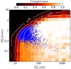Fig. 1.

Completeness in the $θ_{M}^{in}$ $\theta_M^{\rm in}$ versus $S_{int}^{in}$ $S_{\mathrm{int}}^{\mathrm{in}}$ plane as inferred from extensive MC simulations. The completeness given by the color scale represents the fraction of sources recovered by PyBDSF (resolved and unresolved) over the original number of mock sources. The blue points show the position of resolved SFGs in the VLA COSMOS 3 GHz map studied in this work. White contours represent a completeness levels of 5, 25, 50 and 75%.

3.3.1. Selection function, maximum recovered size

To constrain the maximum detectable size of a galaxy as a function of redshift, stellar mass, and Δ log(SSFR)_MS, we explore the angular size of mock sources that were resolved by PyBDSF. The completeness levels in the $θ_{M}^{in}$ $\theta_M^{\rm in}$ versus $S_{int}^{in}$ $S_{\mathrm{int}}^{\mathrm{in}}$ plane (Fig. 1) reveal that the maximum recovered deconvolved FWHM ( $θ_{M}^{max}$ $\theta_M^{\rm max}$ ), for sources within $10^{- 5} Jy < S_{int}^{in} < 10^{- 3} Jy$ $10^{-5}\, {\text{ Jy}} < S_{\text{ int}}^{\text{ in}} < 10^{-3}\,{\text{ Jy}}$ , strongly depends on $S_{int}^{in}$ $S_{\mathrm{int}}^{\mathrm{in}}$ ; i.e., a higher flux density increases the possibility of detecting extended sources¹. Thus, at a given redshift, faint galaxies are preferentially detected if they are compact, while bright starbursting systems are detected even if they are extended. This selection function (i.e., completeness level of 10%) is further discussed in Sects. 4.1 and 4.2.

3.3.2. Upper limit for the size of unresolved sources

A total of 665 SFGs (21%) from our sample are unresolved $(θ_{M}^{out} = 0 arcsec)$ $(\theta_M^{\rm out} = 0 \,{\rm arcsec})$ by PyBDSF. In order to assign an upper limit to their intrinsic angular size $θ_{M}^{in} < θ_{lim}$ $\theta_M^{\rm in} < \theta_{\rm lim}$ , we explore the input size of mock sources retrieved as unresolved in the MC simulations. In Fig. 2, we plot their distribution in the $θ_{M}^{in} - S_{int}^{in}$ $\theta_M^{\mathrm{in}}{-}S_{\mathrm{int}}^{\mathrm{in}}$ plane. Most of the sources retrieved as unresolved by PyBDSF are, as expected, at the faint and compact end of the parameter space tested here. Based on their angular size distribution (Fig. 2, right panel), we find that around 90% of them satisfy the condition: $θ_{M}^{in} \leq θ_{beam}$ $\theta_M^{\rm in} \leq \theta_{\rm beam}$ (blue line). We thus define θ_beam = 0.75 arcsec as the upper limit for the size of the 665 unresolved SFGs in our sample.

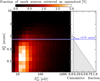Fig. 2.

Left panel: fraction of mock sources retrieved by PyBDSF as unresolved in the $θ_{M}^{in} - S_{int}^{in}$ $\theta_{M}^{\mathrm{in}}{-}S_{\mathrm{int}}^{\mathrm{in}}$ plane showing the ratio of the number of unresolved sources per bin to the total number of unresolved sources in the entire parameter space. Right panel: cumulative size distribution of mock sources retrieved as unresolved, which represent 29% of the total number of sources injected in our MC simulations. Around 90% of them lie below θ_beam = 0.75 arcsec (blue line), hence we use this value as the upper limit for the size of unresolved SFGs in the VLA COSMOS 3 GHz map.

3.3.3. How reliable are the retrieved FWHM and flux density?

It is well known that noise fluctuations boost the flux of faint sources detected in sensitivity-limited astronomical surveys (e.g., Hogg & Turner 1998; Coppin et al. 2005; Casey et al. 2014). It is expected that a similar effect takes place when determining the size of faint and compact sources. Therefore, in a pioneering effort, we use the MC simulations to correct both the FWHM and flux density (and associated uncertainties) provided by PyBDSF. We proceeded as follows:

We create a catalog containing all mock sources retrieved by PyBDSF. Hence, it contains information about the input ( $S_{int}^{in}$ $S_{\mathrm{int}}^{\mathrm{in}}$ , $θ_{M}^{in}$ $\theta_M^{\rm in}$ ) and output parameters ( $S_{int}^{out}$ $S_{\mathrm{int}}^{\mathrm{out}}$ , $θ_{M}^{out}$ $\theta_M^{\rm out}$ ).
All the sources in the catalog are binned in the $S_{int}^{out} - θ_{M}^{out}$ $S_{\mathrm{int}}^{\mathrm{out}} {-} \theta_M^{\mathrm{out}}$ plane (as shown in Fig. 1). For all objects in each bin, we estimate $r_{θ} \equiv (θ_{M}^{out} - θ_{M}^{in}) / σ_{θ}$ $r_{\theta}\equiv(\theta_M^{\rm out}-\theta_M^{\rm in})/\sigma_{\theta}$ and/or $r_{S} \equiv (S_{M}^{out} - S_{M}^{in}) / σ_{S}$ $r_{S}\equiv(S_{\mathrm{M}}^{\mathrm{out}}-S_M^{\mathrm{in}})/\sigma_{S}$ , where σ_θ and σ_S are the uncertainties provided by PyBDSF.
We derive the mean ( μ) and standard deviation (σ) of the r_θ and r_S distributions (Fig. 3). While the value of μ quantifies systematic biases (e.g., “flux boosting”), σ evaluates whether the uncertainties given by PyBDSF are under- or overestimated. In the ideal case where the measured properties and uncertainties are an appropriate description of the input mock sources, the mean ( μ) and standard deviation (σ) of the distribution should be 0 and 1, respectively. Nevertheless, for both FWHM and flux density, μ is generally greater than zero (Fig. 3), meaning that PyBDSF tends to overestimate the size and flux density of mock sources. The value of σ is also heterogeneous across the $θ_{M}^{out} - S_{int}^{out}$ $\theta_M^{\mathrm{out}} {-} S_{\mathrm{int}}^{\mathrm{out}}$ plane (Fig. 3); $σ_{θ}^{ij}$ $\sigma^{ij}_{\theta}$ and/or $σ_{S}^{ij}$ $\sigma^{ij}_{S}$ higher (lower) than 1 suggests that the uncertainty provided by PyPDSF is being underestimated (overestimated).
Under the condition that all r_θ and r_S distributions should have a mean of zero and dispersion of 1, the corrected source properties $(θ_{M}^{' out}, S_{int}^{' out})$ $( \theta_M^{\mathrm{\prime out}},\, S_{\mathrm{int}}^{\mathrm{\prime out}} )$ and associated uncertainties $(σ_{θ}^{'}, σ_{S}^{'})$ $(\sigma_{\theta}^\prime,\, \sigma_{S}^\prime)$ are given by

$\begin{matrix} \begin{matrix} θ_{M}^{' out} = θ_{M}^{out} - μ_{θ}^{ij} \times σ_{θ}, \\ S_{int}^{' out} = S_{int}^{out} - μ_{S}^{ij} \times σ_{S}, \end{matrix}} \end{matrix}$ $\begin{aligned} \left. \begin{aligned} \theta _M^\mathrm{\prime out}=\theta _M^\mathrm{out} - \mu ^{ij}_{\theta }\times \sigma _{\theta }, \\ S_{\rm int}^\mathrm{\prime out}=S_{\rm int}^\mathrm{out} - \mu ^{ij}_{S}\times \sigma _{S}, \end{aligned} \right\} \end{aligned}$ (3)

and

$\begin{matrix} \begin{matrix} σ_{θ}' = σ_{θ}^{ij} \times σ_{θ}, \\ σ_{S}' = σ_{S}^{ij} \times σ_{S}, \end{matrix}}, \end{matrix}$ $\begin{aligned} \left. \begin{aligned} \sigma _{\theta }\prime =\sigma _{\theta }^{ij}\times \sigma _{\theta }, \\ \sigma _{S}\prime =\sigma _{S}^{ij}\times \sigma _{S}, \end{aligned} \right\} ,\end{aligned}$ (4)

where $μ_{θ}^{ij}, μ_{S}^{ij}, σ_{θ}^{ij}$ $\mu^{ij}_{\theta}, \, \mu^{ij}_{S}, \sigma^{ij}_{\theta}$ , and $σ_{S}^{ij}$ $\sigma^{ij}_{S}$ are the mean and standard deviations of the r_θ and r_S distributions in each bin; here i = 1…m and j = 1…n, with m and n the numbers of columns and rows used to grid the $θ_{M}^{out} - S_{int}^{out}$ $\theta_M^{\mathrm{out}} {-} S_{\mathrm{int}}^{\mathrm{out}}$ plane.
After applying our corrections to all mock resolved sources, we retrieve the distribution of r_θ and r_S. By fitting a single-Gaussian component, we find μ = 0.0 and σ = 1.0 for both distributions (Fig. 4). This assures that the corrected flux densities and FWHM, as well as their associated uncertainties, are a good description of the input mock sources. It should be noted that for a small fraction of mock sources, our corrected FWHM is still being underestimated; this gives rise to a wing in the r_θ distribution (Fig. 4). We verified that these outliers are mainly located at the extended and bright end of the $θ_{M}^{out} - S_{int}^{out}$ $\theta_M^{\mathrm{out}} {-} S_{\mathrm{int}}^{\mathrm{out}}$ plane ( $θ_{M}^{out} > 0.75 arcsec$ $\theta_M^{\rm out} > 0.75\,{\rm arcsec}$ and $S_{int}^{out} > 0.1 mJy$ $S_{\mathrm{int}}^{\mathrm{out}} > 0.1\mathrm{mJy}$ ) where less than 1% of SFGs in our final sample reside (see Fig. 1).
To correct the measured flux density of unresolved sources, we compare the input and output flux density of mock sources retrieved as unresolved by PyBDSF (see Fig. A.1). We then derive flux boosting factors as a function of S/N; at S/N = 5 the flux density is overestimated by 17%, while at S/N > 7 the effect of flux boosting is negligible.
We verified that the corrections and the completeness do not strongly depend on the input angular size and flux density distribution used in the MC simulations. A uniform distribution (equal number of sources per bin in the $θ_{M}^{in} - S_{int}^{in}$ $\theta_M^{\mathrm{in}} {-} S_{\mathrm{int}}^{\mathrm{in}}$ plane) yields correction factors that are consistent with those obtained from a realistic input distribution.

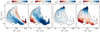Fig. 3.

Systematic errors and uncertainties for the FWHM (left two panels) and flux density (right two panels) of mock sources in the $θ_{M}^{out} - S_{int}^{out}$ $\theta_{M}^{\mathrm{out}}{-}S_{\mathrm{int}}^{\mathrm{out}}$ plane covered by 2519 resolved SFGs studied in this work. Contour levels showing the distribution of these sources are at 1, 5, 50, 250 sources per bin. Positive (negative) values of $μ_{θ}^{ij}$ $\mu^{ij}_{\theta}$ and $μ_{S}^{ij}$ $\mu^{ij}_{S}$ indicate that the measured quantity is overestimated (underestimated). Values of $σ_{θ}^{ij}$ $\sigma^{ij}_{\theta}$ and/or $σ_{S}^{ij}$ $\sigma^{ij}_{S}$ higher (lower) than 1 suggest that the uncertainty of the measured parameter is being underestimated (overestimated).

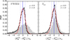Fig. 4.

Distribution of sigma deviations for the FWHM (left panel) and integrated flux density (right panel) of all mock sources. The distribution that is produced from the corrected quantities is shown in black, while in gray that obtained from the measured quantities given by PyBDSF. A single-component Gaussian fit is shown in red. For both corrected distributions, we find the best fitting parameters of μ = 0 and σ = 1 (blue solid and dashed lines), which indicates that the corrected flux density and FWHM (and associated uncertainties) are a proper description of the mock sources. Blue solid (dashed) lines illustrate the locus of μ = 0 (σ = 1).

After validating our method, we then derived the corrected flux density and size of SFGs in our sample. In Fig. 5, we compare the flux and FWHM before and after revision in order to illustrate the effect of our corrections. Both flux and size measurements appear to be overestimated for faint radio sources. This result is expected as positive noise fluctuations enhance the flux density on a pixel-by-pixel basis and, consequently, the amplitude and variance of a 2D Gaussian model are magnified. This phenomenon translates into a flux boosting factor of ∼20% at the faint end (see right panel of Fig. 5), which is comparable with the uncertainty on the flux density of a 5σ radio source detection. On the other hand, “size boosting” seems to be ubiquitous for faint and compact sources that have a deconvolved FWHM smaller than the size of the synthesized beam (see left panel of Fig. 5). This can be attributed to the large uncertainties associated with the deconvolution process of slightly resolved and faint radio sources.

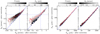Fig. 5.

Comparison between observed and corrected source parameters of SFGs in the sample. Left panels: FWHM of 2519 resolved sources before and after correction, color-coded by number counts and median flux density. The red solid (dashed) lines show the 50th (16th, 84th) percentile of the FWHM values prior correction, using a 0.05 dex bin width along the x-axis. The dotted blue lines illustrate the FWHM of the synthesized beam (0.75 arcsec), while the 1:1 relation is shown by the blue dashed line. Right panels: flux density of 3184 SFGs (resolved and unresolved) before and after correction, color-coded by number counts and median FWHM. The red solid (dashed) lines show the 50th (16th, 84th) percentile of the flux density values prior correction, using a 0.1 dex bin width along the x-axis. The 1:1 relation is shown by the blue dashed line.

As a consistency test, we compare our corrected flux density measurements with those reported by Smolčić et al. (2017b), which were derived following a non-parametric approach with blobcat. By considering both resolved and unresolved sources (see Fig. A.2), we found that the two quantities are, on average, consistent.

3.4. From flux and size measurements to SFR and effective size estimates

We estimate the total SFR by adding the estimates from the infrared (SFR_IR) and uncorrected UV emission (SFR_UV), allowing us to account for the dust obscured and unobscured star formation activity. We use the Kennicutt (1998) calibration and the infrared–radio correlation (e.g., Magnelli et al. 2015; Delhaize et al. 2017) to derive SFR_IR as

$\begin{matrix} {SFR}_{IR} [M_{⊙} {yr}^{- 1}] = f_{IMF} 10^{- 24} 10^{q_{IR}} L_{1.4 GHz} [W {Hz}^{- 1}], \end{matrix}$ $\begin{aligned} \mathrm{SFR}_{\rm IR} \, [M_\odot \,\mathrm{yr}^{-1}]= f_{\rm IMF}10^{-24}10^{q_{\rm IR}}L_{\rm 1.4\,GHz} \, [\mathrm{W\,Hz^{-1}}], \end{aligned}$ (5)

where f_IMF = 1.72 for a Salpeter initial mass function (IMF) and q_IR is parametrized as a function of redshift (for SFGs only) as q_IR = (2.83 ± 0.02) × (1 + z)^{−0.15 ± 0.01} (Delhaize et al. 2017). The value of L_1.4 GHz, on the other hand, can be derived from the observer-frame 3 GHz fluxes (S_{ν_3 GHz} [W Hz⁻¹ m⁻²]) through

$\begin{matrix} L_{1.4 GHz} = \frac{4 π D_{L} {(z)}^{2}}{{(1 + z)}^{1 - α}} {(\frac{1.4}{3})}^{- α} S_{3 GHz}, \end{matrix}$ $\begin{aligned} L_{\rm 1.4\,GHz}=\frac{4\pi D_{\rm L}(z)^2}{(1+z)^{1-\alpha }}\left(\frac{1.4\,}{3}\right)^{-\alpha }S_{3\, \mathrm{GHz}}, \end{aligned}$ (6)

where D_L is the luminosity distance in meters and α is the spectral index of the synchrotron power law (S_ν ∝ ν^−α) of 0.8 (Condon 1992).

We also use the near-UV (NUV) emission of galaxies from the COSMOS2015 catalog (Laigle et al. 2016) to estimate SFR_UV as follows (Kennicutt & Evans 2011):

$\begin{matrix} {SFR}_{UV} = 10^{- 43.17} L_{NUV} [erg s^{- 1}] . \end{matrix}$ $\begin{aligned} \mathrm{SFR_{UV}}= 10^{-43.17} L_{\rm NUV} \, [\mathrm{erg\, s^{-1}}]. \end{aligned}$ (7)

Finally, to compare our radio continuum size estimates with those derived from the optical/UV, we convert our θ_M measurements into effective radius (R_eff), i.e., the radius enclosing half of the total flux density. To this end, we assume that most of our galaxies are star-forming disks with an exponentially declining surface brightness distribution. This is consistent with the average Sérsic index of n ∼ 1 for MS galaxies (e.g., Nelson et al. 2016b) and luminous sub-mm selected galaxies (SMGs; Hodge et al. 2016), preferentially located above the MS. Under this assumption, Murphy et al. (2017) have analytically proven that for slightly resolved radio sources (with R_eff ≲ θ_beam) θ_M and R_eff can be related by

$\begin{matrix} θ_{M} \approx 2.430 R_{eff} . \end{matrix}$ $\begin{aligned} \theta _M\approx 2.430 R_{\rm eff}. \end{aligned}$ (8)

3.5. Final sample

We distributed the 3184 SFGs in our sample in five redshift bins following those presented by Laigle et al. (2016): [0.35, 0.65], [0.65, 0.9], [0.9, 1.35], [1.35, 1.7], and [1.75, 2.25]. This allows us to directly use the stellar mass completeness limits (per redshift bin) of the COSMOS2015 catalog, and hence assemble a mass-complete sample of radio-selected SFGs in the COSMOS field. The number of SFGs per redshift bin is nearly homogeneous (with a median of ∼650 sources). Given the small comoving volume probed by COSMOS at low redshift and the selection function that restricts our parameter space to compact starburst galaxies, we are not able to explore the size evolution of SFGs in the redshift regime below z = 0.35.

In Fig. 6, we present the sample of 3184 SFGs in the SFR−M_⋆−z plane. The bulk of the radio-selected SFGs is consistent with the position and dispersion of the MS of SFGs, as given by Schreiber et al. (2015). At the low-mass end, however, our radio detection limit biases our sample towards the starburst population. Since we aim to statistically analyze the size distribution of SFGs on and above the MS, we need to focus on the high-mass end. For this purpose, we define a mass-limit ( $M_{⋆}^{lim}$ $M_\star^{\rm lim}$ ) for each redshift bin, above which we are able to consistently probe both SFGs on (−0.3 ≤ Δ log(SSFR)_MS ≤ 0.3) and above the MS (Δ log(SSFR)_MS > 0.3). By considering systems with $M_{⋆} > M_{⋆}^{lim}$ $M_\star > M_\star^{\rm lim}$ we are also able to assemble a mass-complete sample of radio-selected SFGs, given that in all redshift bins $M_{⋆}^{lim}$ $M_\star^{\rm lim}$ is higher than the stellar mass completeness limit of the COSMOS2015 catalog.

4. Results

In this section, we explore the dependence of the radio continuum size (R_eff) on the stellar mass, distance to the MS and redshift. We carefully address these relations while keeping in mind the completeness and size biases mentioned in Sect. 3.3 and that our analysis is restricted to $M_{⋆} > M_{⋆}^{lim}$ $M_\star > M_\star^{\rm lim}$ , i.e., the part of the parameter space where the sample of SFGs on and above the MS is complete. We also verified that the trends presented below remain even if we use uncorrected measurements (see Appendix B).

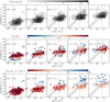Fig. 6.

Upper panels: sample of 3184 SFGs in the SF–M_⋆ − z plane, color-coded for the number of sources per bin. Shown are the positions of the MS of SFGs (black lines) and the associated dispersion (dashed black lines) given by Schreiber et al. (2015). Vertical red lines show the mass limit above which we consistently probe SFGs on and above the MS. Middle and lower panels: median size and star formation surface density, respectively, of the 3184 SFGs in the sample. We use 1000 MC realizations to include the values for unresolved sources, which are drawn from the distributions described in Sects. 4.2 and 4.4.

4.1. Radio continuum size versus stellar mass

The stellar mass-size relation in galaxies (e.g., Furlong et al. 2017; Allen et al. 2017) is thought to be linked to the physical processes that regulate galaxy assembly, such as galaxy minor and major mergers and gas accretion (e.g., Khochfar & Silk 2006, 2009; Dekel et al. 2009; Oser et al. 2010; Gómez-Guijarro et al. 2018). Thus, it is a fundamental ingredient to understand galaxy evolution.

Here, we attempt to characterize the stellar mass–radio size relation up to z = 2.25. We thus explore the scatter of SFGs in the R_eff−M_⋆ plane by deriving their density distribution per stellar mass bin (0.5 dex width; Fig. 7). We use 10 000 Monte Carlo trial model runs to take into account the dispersion introduced by the uncertainties and upper limits of R_eff for resolved and unresolved sources, respectively. Based on our MC simulations (Fig. 2), the size of unresolved sources can be drawn from a uniform distribution in log space within the range $[0.1, R_{eff}^{\lim}] kpc$ $[0.1, R_{\mathrm{eff}}^{\mathrm{lim}}]\, \mathrm{kpc}$ , where $R_{eff}^{\lim}$ $R_{\mathrm{eff}}^{\mathrm{lim}}$ is the upper limit for the source size. We also derived the median size of SFGs through the Kaplan–Meier (KM) estimator (Kaplan & Meier 1958), which allows us to take into account the upper limits for the size of unresolved sources. We find that the two methods, MC realizations and KM estimator, yield consistent results (Fig. 7). In all redshift bins, the size distribution of SFGs remains constant over the range of stellar mass probed here, where the median size differs by less than 25% (see Table C.1). Qualitatively, this result is consistent with the shallow slope (α_opt/UV) of the stellar mass and optical/UV size relation of SFGs (α_opt/UV ∼ 0.2; e.g., van der Wel et al. 2014; Mowla et al. 2018). Finally, we checked that this relation remains if we use two separate samples of SFGs: one composed of galaxies on the MS (−0.3 ≤ Δ log(SSFR)_MS ≤ 0.3) and another above it (Δ log(SSFR)_MS > 0.3).

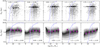Fig. 7.

Upper panels: sample of 3184 SFGs in the R_eff−M_⋆−z plane. The blue solid line shows the maximum size, corresponding to the 10% completeness level, that can be observed for a galaxy with Δ log(SSFR)=0 evaluated at the central redshift value per bin. Blue dashed lines show the mass limit above which we consistently probe SFGs on and above the MS. Black arrows show the upper limits for the size of unresolved sources. Lower panels: density distribution per stellar mass bin (0.5 dex width) of SFGs in the R_eff−M_⋆−z plane. Contour levels are at the 10, 20, 30, 40, 50, 60, 70, 80, and 90th percentiles. The median size derived via the KM estimator is shown by the dark magenta circles, the error bars correspond to the 16th and 86th percentiles of the distribution.

We still have to consider that the last result might be affected by our selection function. As mentioned in Sect. 3.3, galaxies are preferentially detected if they are compact, especially at the faint end. This could yield a misleading stellar mass–radio size relation, as low-mass SFGs are fainter than their massive counterparts (due to the MS slope, Fig. 6). To quantify this possible bias, we use the output of our MC simulation to estimate the maximum recoverable size as a function of stellar mass as follows. At a given redshift bin and for each mass, we infer the SFR of a galaxy with Δ log(SSFR)_MS = 0. Then we convert this SFR into flux density using the central redshift of the bin. Finally, this flux is associated with a maximum recoverable size using our 10% completeness limit in the $θ_{M}^{in} - S_{int}^{in}$ $\theta_M^{\mathrm{in}}{-}S_{\mathrm{int}}^{\mathrm{in}}$ plane (Sect. 3.3.1). As observed in Fig. 7, this selection function hinders the detection of extended SFGs with stellar mass below and near $M_{⋆}^{\lim}$ $M_{\star}^{\mathrm{lim}}$ ; however, it does not affect the parameter space above log(M_⋆/M_⊙) = 10.5. Hence, the negligible dependence of the stellar mass on the radio size of SFGs with log(M_⋆/M_⊙) > 10.5 remains unaffected by our selection.

4.2. Radio continuum size of SFGs on and above the main sequence

Since both the size and Δ log(SSFR)_MS of SFGs can be discussed within the context of gas accretion and merger-driven star formation (e.g., Elbaz et al. 2011, 2018; Lang et al., in prep.), it is essential to characterize their interplay in detail. We therefore take advantage of our mass-complete sample of radio-selected SFGs to systematically explore their size distribution as a function of Δ log(SSFR)_MS and cosmic time (Fig. 8). We recall that we consider SFGs with $M_{⋆} > M_{⋆}^{lim}$ $M_\star > M_\star^{\rm lim}$ , which is the region of the parameter space where we can consistently probe galaxies on and above the MS.

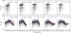Fig. 8.

Upper panels: star-forming galaxies with $M_{⋆} > M_{⋆}^{lim}$ $M_\star > M_\star^{\rm lim}$ in the size−Δ log(SSFR)−z plane. The blue solid line shows the maximum size, corresponding to the 10% completeness level, that can be observed for a galaxy with $M_{⋆} = M_{⋆}^{lim}$ $M_\star\,{=}\,M_\star^{\rm lim}$ evaluated at the central redshift value per bin. Black arrows show the upper limits for the size of unresolved sources. Lower panels: density distribution per Δ log(SSFR) bin (0.5 dex width) of SFGs in the size−Δ log(SFSR)−z plane. Contour levels are at the 10, 20, 30, 40, 50, 60, 70, 80, and 90th percentiles. The median size derived via the KM estimator is shown by the dark magenta circles, the error bars correspond to the 16th and 86th percentiles of the distribution.

Similarly to the previous section, we derive the median size of SFGs per Δ log(SSFR)_MS bin following a MC approach and using the KM estimator. As observed in Fig. 8, the two methods agree well and reveal a trend where SFGs with higher Δ log(SSFR)_MS values are compact, in particular at lower redshifts where this tendency is more pronounced. The median size of z ∼ 0.5 (z ∼ 2) MS galaxies is 4 (2) times larger than those with Δ log(SSFR)_MS > 0.9 (see Table C.2). We note that although SFGs on the MS are preferentially extended (median R_eff ∼ 1.5 ± 0.2 kpc), some can be as compact as galaxies with elevated Δ log(SSFR)_MS.

To verify that our selection function does not bias these trends, we estimate the maximum recoverable size as a function of Δ log(SSFR)_MS. At a given redshift bin and for each Δ log(SSFR)_MS, we infer the SFR of a galaxy with $M_{⋆} = M_{⋆}^{lim}$ $M_\star\,{=}\,M_\star^{\rm lim}$ evaluated at the central redshift of the bin. We then convert this SFR into flux density and associate it to a maximum recoverable size using our completeness in the $θ_{M}^{in} - S_{int}^{in}$ $\theta_M^{\mathrm{in}}{-}S_{\mathrm{int}}^{\mathrm{in}}$ plane (Sect. 3.3.1). As inferred from Fig. 8, while the selection function does not affect the size distribution of SFGs above the MS, it does hamper the detection of extended SFGs on and below the MS. We note that retrieving these missing systems would only strengthen the anti-correlation between the median size of SFGs and Δ log(SSFR)_MS.

The size dichotomy of SFGs on and above the MS is consistent with the results of Elbaz et al. (2011) and Rujopakarn et al. (2016). They did not report, however, that compact galaxies can be “hidden” within the MS (Fig. 8), which is in agreement with recent high-resolution observations of z ∼ 2 SFGs (e.g., Elbaz et al. 2018; Lang et al. in prep.). This effect is related to the stacking approach followed by Elbaz et al. (2011), which can only provide median quantities, and the small sample of Rujopakarn et al. (2016), which might be affected by incompleteness.

In general, these findings support the emerging consensus where the global star-forming region of SFGs on the MS is preferentially but not exclusively extended, while SFGs above the MS are always more compact systems.

4.3. Size of SFGs in different wavelengths and its evolution with redshift

We now explore the radio continuum size evolution of SFGs over the redshift range 0.35 < z < 2.25 to better constrain the processes regulating the growth of galaxies. In addition, through the comparison of the size–redshift relation as traced by stellar light, dust, and supernova remnants, we investigate where and how new stars are formed in galaxies. To this end, we select galaxies from our final sample (Sect. 3.5) with log(M_⋆/M_⊙)> 10.5, which is the only mass bin consistently probed across the redshift range explored here. For all the redshift bins, we then derive the median R_eff (via the KM estimator) of SFGs on and above the MS, i.e., −0.3 ≤ Δ log(SSFR)_MS ≤ 0.3), and (Δ log(SSFR)_MS > 0.3), respectively. As illustrated in Fig. 9, the radio continuum size of both SFG populations remains nearly constant across cosmic time. By using a parametrization of the form R_eff ∝ (1 + z)^α, we find a slope of only −0.26 ± 0.08 (0.12 ± 0.14) for SFGs on (above) the MS. As expected from the results in Sect. 4.2, the median size of SFGs on the MS (R_eff = 1.5 ± 0.2 kpc) is significantly larger than for those above it (R_eff = 1.0 ± 0.2 kpc).

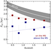Fig. 9.

Radio continuum size (in terms of half-light radius, R_eff) of galaxies on and above the MS as a function of redshift. Only SFGs with log(M_⋆/M_⊙) > 10.5 are included. Filled data points (squares and circles) show the median size for SFGs (above and on the MS) in the different redshift bins probed in this work. Vertical bars show the 95% interval confidence of the median, while horizontal bars represent the redshift bin width. Gray shaded region illustrates the growth curve derived in the UV-optical for UV-luminous SFGs given by R_eff/kpc = (4.78 ± 0.68)(1 + z)^{(−0.84 ± 0.11)} (Shibuya et al. 2015). Red and blue dotted lines show the linear fit to parametrize the redshift evolution of the median radio continuum size as R_eff/kpc = (2.1 ± 0.2)(1 + z)^{(−0.26 ± 0.08)} and R_eff/kpc = (0.6 ± 0.4)(1 + z)^{(0.12 ± 0.14)} for SFGs on and above the MS, respectively.

The size evolution presented here is still influenced by two factors that cannot be characterized with the available data:

First, our radio continuum size estimates trace different rest-frame frequencies, from 4 GHz at z = 0.35 to 9.7 GHz at z = 2.25. Since higher energy electrons lose energy more rapidly, their propagation throughout the galaxy is more limited than their low-energy counterparts (e.g., Kobayashi et al. 2004); 3 GHz emitting electrons, in particular, are expected to diffuse ∼25% farther into the ISM than those at 10 GHz (Murphy et al. 2017). Thus, the observed radio continuum synchrotron emission would tend to be more concentrated as the redshift increases. This phenomenon does not significantly affect the trends presented above as a 25% larger radio size at z = 2.25 would lead to α ∼ −0.10 (∼0.25) for SFGs on (above) the MS.
Second, given the limited number of resolution elements across the SFGs in the sample, we cannot assess their radio continuum surface brightness distribution and determine R_eff. Therefore, we converted the deconvolved FWHM to R_eff (following Murphy et al. 2017) assuming that most of our SFGs follow an exponentially declining surface brightness distribution (with Sérsic index n = 1). Naturally, such a conversion might deviate from the true R_eff on a galaxy-by-galaxy basis, especially for SFGs above the MS that tend to have cuspier light profiles (e.g., Wuyts et al. 2011). For slightly resolved sources, like the ones presented here, we do not expect major changes in R_eff if the Sérsic index is larger than 1. For example, even for 0.2 arcsec resolution dust-continuum observations, Elbaz et al. (2018) report that R_1/2 ≡ 0.5 × FWHM and R_eff are both equally good proxies for the half-light radius, either leaving the index free or fixed to 1.

4.3.1. Comparison with other radio continuum size estimates

Bondi et al. (2018) have independently derived the R_eff of radio sources detected in the VLA COSMOS 3 GHz map (Smolčić et al. 2017a), including AGN and SFGs up to z ∼ 3. They assembled a sample of SFGs that is complete in L_3 GHz over 0.8 < z < 3 with median log(M_⋆/M_⊙)=10.6; no distinction was made between on and off MS galaxies. For this sample, the size of SFGs marginally increases with cosmic time, from median ∼1.4 kpc at z = 2.1 to R_eff ∼ 1.6 kpc at z = 0.8. This is in agreement with the shallow size evolution of MS galaxies in our sample (which corresponds to ∼90% of all SFGs) with median R_eff = 1.5 ± 0.1 kpc, within the same redshift range and comparable stellar mass. We note that despite the independent methodologies used to measure radio sizes in the μJy regime, and different selection criteria, our median sizes are consistent. Bondi et al. (2018) used, in particular, the original and convolved images (up to a resolution of 2.2 arcsec) of the VLA COSMOS 3 GHz mosaic and took the flux density provided by blobcat as a prior in their 2D Gaussian fitting procedure. This flux prior limits the effect of size boosting, leading to comparable size measurement between our two studies. On the other hand, by using the VLA COSMOS 3 GHz map, Miettinen et al. (2017) reported a median R_eff ∼ 1.9 kpc for 152 SMGs over the redshift range of 1 ≲ z ≲ 6. The discrepancy of ∼35% between the Miettinen et al. (2017) value of R_eff and that reported here at z = 2.25 and in Bondi et al. (2018) is likely driven by the different selection criteria.

The angular size of the μJy radio sources has also been recently explored in different extragalactic deep fields. At the same frequency, 3 GHz, it was found that z ∼ 1 SFGs in the Lockman-Hole have a median effective radius of ∼1.0 kpc (Cotton et al. 2018), which agrees with the median size of SFGs above the MS derived here (see Fig. 9). Murphy et al. (2017) have reported that z ∼ 1.2 GOODS-N SFGs have a median R_eff of only ∼0.5 kpc at 10 GHz. This small size could be associated with selection effects as the high-resolution 10 GHz observations (0.22 arcsec) are sensitive to smaller angular scales. Additionally, as stated by Murphy et al. (2017), the discrepancy between 3 GHz and 10 GHz radio sizes is driven by the frequency-dependent cosmic ray diffusion. This physical phenomenon could partially explain the large median R_eff of 2.3 ± 0.6 kpc at 1.4 GHz of z ∼ 1.5 SFGs (in the Hubble Deep Field; Lindroos et al. 2018), which is ∼1.5 times larger than the median size at 3 GHz of galaxies in our sample. On the contrary, the larger energy loss rate at higher frequencies cannot explain the large median R_eff of ∼2.7 kpc (FWHM ∼ 0.8 arcsec) at 5.5 GHz reported for SFGs at similar redshift (in GOODS-N; Guidetti et al. 2017). Finally, we note that (apart from the frequency and resolution of the observations) a more general issue about size determination is related to the surface brightness limit of each survey. As inferred from Fig. 1, a lower rms sensitivity hampers the maximum detectable angular size, biasing the sample towards more compact radio sources.

4.3.2. Comparison with FIR, optical, and Hα sizes

It has been reported that the FIR size of z ∼ 2 SFGs is, on average, ∼1.5 kpc (e.g., Rujopakarn et al. 2016; Elbaz et al. 2018, Lang et al. in prep.), which is consistent with the median radio size of SFGs reported here. Extinction-corrected Hα radial profiles tracing the global star-forming region of z ∼ 1.4 SFGs yield a median effective radius of <1 kpc (with 9.8 < log(M_⋆/M_⊙) < 11; Nelson et al. 2016a), comparable with the radio continuum sizes of SFGs above the MS. In contrast, the median effective radius derived from uncorrected Hα emission is 4.2 ± 0.1 kpc for SFGs at z ∼ 1 and similar stellar mass (Nelson et al. 2012). This disparity is related to the high dust content in massive galaxies; if star formation is highly obscured at small radii, Hα emission would appear less centrally concentrated, and the inferred effective radius will thus be larger (e.g., Möllenhoff et al. 2006; Nelson et al. 2016a,b).

In Fig. 9, we also present a comparison of the size of SFGs as observed from radio continuum and optical to UV throughout cosmic time. We use the size evolution derived by Shibuya et al. (2015) via broadband optical imaging with the Hubble Space Telescope (HST). In this case, we adopt the median fit obtained for the UV bright galaxies (−24 < M_UV < −21) corresponding to the stellar mass range of 10 < log(M_⋆/M_⊙) < 11, which is consistent with the mass range of SFGs used in this work. Given that Shibuya et al. (2015) masked star-forming clumps, their size estimates can be used as a proxy for the stellar mass distribution of galaxies. As revealed by Fig. 9, the overall star-forming region of SFGs (on and above the MS) is more compact than their stellar component. In particular, at z = 0.5 (2) the optical to UV emission is ∼2 (1.3) times more extended than the radio continuum. Since these HST-based estimates are not corrected for extinction, it is likely that (similar to what has been shown for Hα sizes) the optical to UV effective radius is overestimated. Given that dust extinction becomes substantial in high-redshift galaxies (e.g., Leslie et al. 2018), we would expect that their optical to UV size is overestimated by a larger fraction than those galaxies at lower redshifts. Correcting for this effect could alleviate the discrepancy between the extent of the stellar and star-forming component of galaxies at high redshift.

In summary, radio continuum, FIR, and extinction-corrected Hα emission suggest that star formation occurs in smaller regions relative to the total stellar component (e.g., Simpson et al. 2015; Rujopakarn et al. 2016; Fujimoto et al. 2017; Elbaz et al. 2018; Karoumpis et al., in prep.). Here, in particular, we find that while the radio continuum size remains nearly constant, that inferred from optical to UV emission increases with cosmic time. In Sect. 5.2, we discuss this finding further within the context of bulge growth.

4.4. Cosmic evolution of Σ_SFR

From numerical simulations, SFGs are expected to experience a compaction phase while the SFR increases and they move towards the upper end of the MS (e.g., Tacchella et al. 2016). This scenario can now be tested through our radio continuum size estimates. We thus derive the galactic-average SFR surface density, $Σ_{SFR} = SFR / 2 π R_{eff}^{2}$ $\Sigma_{\rm SFR}={\rm SFR}/2\pi R_{\rm eff}^2$ , and use it to evaluate how concentrated the star formation activity in galaxies is as they evolve across the MS (see Figs. 6 and 10). In calculating Σ_SFR we assume that the total SFR (SFR_IR + SFR_UV) is confined within the radio continuum-based R_eff. This simplification is valid as the UV-based SFR is considerably low for massive, high-redshift SFGs (e.g., Buat et al. 2012); therefore, the star formation activity is mainly traced by the radio continuum (unobscured) emission.

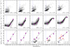Fig. 10.

Upper panels: star-forming galaxies with $M_{⋆} > M_{⋆}^{lim}$ $M_\star > M_\star^{\rm lim}$ in the Σ_SFR − Δ log(SSFR)−z plane. Dashed blue lines show the Δ log(SSFR) limit of −0.3 above which our sample of SFGs is complete in terms of distance to the MS. Black arrows show the upper limits for the size of unresolved sources. Middle panels: density distribution per Δ log(SSFR) bin (0.4 dex width) of SFGs in the Σ_SFR−Δ log(SSFR)−z plane. Contour levels are at the 10, 20, 30, 40, 50, 60, 70, 80, and 90th percentiles. The median size derived via the KM estimator is shown by the dark magenta circles; the error bars correspond to the 16th and 86th percentiles of the distribution. Lower panels: power law describing the Σ_SFR−Δ log(SSFR) relation (dotted black line). The slope and normalization are given in the lower right corner. The median size derived via the KM estimator is also shown by the dark magenta circles. For comparison, we present the compilation of SFGs from Genzel et al. (2010, black filled circles), Tacconi et al. (2013, black empty squares), Elbaz et al. (2018, red pentagons), and Lang et al. (in prep., orange triangles). The black arrow illustrates the factor to be considered when comparing Σ_SFR of galaxies in our sample with that reported by Genzel et al. (2010) and Tacconi et al. (2013) (see text for details).

As in Sects. 4.1 and 4.2, we follow a MC approach to derive the distribution of Σ_SFR per Δ log(SSFR)_MS bin (Fig. 10); again, only galaxies with $M_{⋆} > M_{⋆}^{lim}$ $M_\star > M_\star^{\rm lim}$ are included in the analysis. In this case, the Σ_SFR for unresolved sources is drawn from a uniform logarithmic distribution within the range [Σ_SFR(R_lim), Σ_SFR(0.1 kpc)]. We verify the reliability of this approach by using the KM estimator (Table C.3). At all redshifts and for both methods, there is a positive relation between Σ_SFR and Δ log(SSFR)_MS that can be described with a power law,

$\begin{matrix} log (Σ_{SFR}) = α \times Δ log {(SSFR)}_{MS} + β, \end{matrix}$ $\begin{aligned} \log (\Sigma _{\rm SFR})=\alpha \times \Delta \log (\mathrm{SSFR})_{\rm MS}+\beta , \end{aligned}$ (9)

where α and β are the slope and normalization, respectively. We use a least-squares (Levenberg–Marquardt) algorithm to fit a linear function to Δ log(SSFR)_MS and derive the best-fitting values for α and β. This procedure is done for each MC realization, while restricting our parameter space to Δ log(SSFR)_MS > −0.3 where our sample is complete. The final values for α and β, shown in Fig. 10, correspond to the median (and 16th and 84th percentiles) after executing 1000 MC trial model runs. While the normalization of the log(Σ_SFR)−Δ log(SSFR)_MS relation decreases with redshift, the value of α reveals that this trend becomes shallower at higher redshift. At z ∼ 2, the difference between Σ_SFR of galaxies on and above the MS is smaller than in the local Universe.

Spatially resolved studies of local SFGs have also reported more centrally peaked radial profiles of Σ_SFR as the distance to the MS increases (Ellison et al. 2018). It has been found that the FIR surface density evolves across the MS with a logarithmic slope of 2.6 (Lutz et al. 2016), which is consistent with the value we derived at z ∼ 0.5 (α = 2.6) using the radio continuum emission. Likewise, from Hα resolved maps it has been shown that z ∼ 1 SFGs follow this relation with α ∼ 1.1 (Magdis et al. 2016), which is ∼50% lower than that reported in this work. This tendency can also be inferred from the Σ_SFR, M_⋆, and SFR of 1 ≲ z ≲ 3 SFGs reported by Genzel et al. (2010) and Tacconi et al. (2013). As presented in Fig. 10, these SFGs also exhibit higher Σ_SFR as the distance to the MS increases, yet their Σ_SFR values appear systematically lower than those reported here. This could be a consequence of the optical-/UV-/Hα-/CO-based size estimates used by the authors, which are larger than those obtained from radio continuum emission (Sect. 4.3.2). If we scale their Σ_SFR values by using our R_opt/R_radio ratios, they increase by a factor of ∼0.7 (0.4) dex at redshift 1.5 (2), which would alleviate this observed discrepancy. Finally, in Fig. 10 we present the sample of SFGs from Elbaz et al. (2018) and Lang et al. (in prep.). Although z ∼ 1.5 SFGs also follow a positive relation between log(Σ_SFR) and Δ log(SSFR)_MS, those at z ∼ 2 are widely scattered. As reported by Elbaz et al. (2018), z ∼ 2 SFGs with starburst-like Σ_SFR are also found close to or within the MS. According to our results, there is a fraction of MS galaxies for which Σ_SFR is significantly higher than expected from the log(Σ_SFR)−Δ log(SSFR)_MS relation. These high-Σ_SFR MS galaxies are present at all redshifts and comprise less than 10% of the MS galaxy population (see contour levels of Fig. 10).

5. Discussion

5.1. Cold gas accretion versus merger mode of star formation

We revealed that most SFGs (log(M_⋆/M_⊙) > 10.5) follow a linear relation in the log(Σ_SFR)−Δ log(SSFR)_MS plane over the redshift range 0.35 < z < 2.25. To the first order, these results can be discussed within the context of the Kennicutt–Schmidt (KS) relation (Σ_SFR−Σ_gas; Kennicutt 1998). We therefore use the scaling relations of Genzel et al. (2015) to derive the typical molecular gas mass of galaxies at three different Δ log(SSFR)_MS bins, namely [−0.3,0.3], [0.3,0.6], and [0.9, 2.0] (see Fig. 10). Then we assume that our radio size estimates (Table C.2) also trace the extent of the molecular gas reservoir; these estimates are subsequently used to approximate the galactic averaged molecular gas density (Σ_mol gas = M_mol gas/2πR_eff). This information is combined with the Σ_SFR values presented in Table C.3, allowing us to approximate the shape of the KS relation (see Fig. 11). It is reassuring that our data points, which cover a wide range in redshift and Δ log(SSFR)_MS, agree within the uncertainties with the KS relation presented by Genzel et al. (2010). Moreover, our data points are consistent with the scenario wherein low- and high-redshift SFGs follow a similar molecular gas–star formation relation (Bouché et al. 2007; Genzel et al. 2010). By considering SFGs with −0.3 ≲ Δ log(SSFR)_MS ≲ 0.9, we derive a super-linear slope of 1.3 ± 0.1. If SFGs with Δ log(SSFR)_MS > 0.9 are included, the slope becomes steeper (1.5 ± 0.1), which indicates that SFGs evolve towards a more efficient regime of star formation as Δ log(SSFR)_MS increases. This is consistent with the small size, and hence higher Σ_SFR, of galaxies above the MS (Fig. 8), which could be the result of gas-rich mergers (e.g., Moreno et al. 2015; Wellons et al. 2015) and/or violent disk instability (VDI; e.g., Dekel & Burkert 2014; Tacchella et al. 2016; Wang et al. 2019).

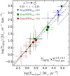Fig. 11.

Star formation rate surface density (Σ_SFR) as a function of the molecular gas surface density (Σ_mol gas). The data points show the locus of the median Σ_SFR and Σ_mol gas of galaxies binned in Δ log(SSFR)_MS and redshift (see Fig. 10). The symbol size increases with redshift, while the color indicates the median Δ log(SSFR)_MS. The solid gray line shows the KS relation reported by Genzel et al. (2010), adapted for a Salpeter IMF. The dotted black line illustrates the best linear fit to all the data points; the dashed thin line shows the best linear fit when we exclude SFGs with Δ log(SSFR)_MS > 0.9. Error bars represent the 16th and 84th percentiles of the inferred Σ_SFR and Σ_mol gas distributions. The molecular gas mass has been approximated by using the prescription of Genzel et al. (2015, see Table 4), where M_mol gas = M_mol gas(z, SSFR, M_⋆ = 10^{10.5 ± 0.5}M_⊙).

Beyond the broad picture of galaxy evolution discussed above, we also reported the discovery of MS galaxies harboring starburst-like Σ_SFR conditions (Fig. 10). This result echoes, in particular, that of Elbaz et al. (2018), who reported the presence of hidden starbursts within the MS at z ∼ 2. Then the fundamental question arises: what is the physical mechanism responsible for high-Σ_SFR MS galaxies? First, these systems could be a result of large cold gas reservoirs distributed over small disk radii (Wang et al. 2019) that, due to disk instability episodes (e.g., Dekel & Burkert 2014), yield high Σ_SFR. If the gas replenishment occurs when a galaxy lies at the lower envelope of the MS (i.e., Δ log(SSFR)_MS ∼ −0.3), the SFR enhancement might not suffice to bring the galaxy above the MS. Second, high-Σ_SFR MS galaxies could be explained in the context of merger-driven bursts of star formation where, depending on the gas content, mergers could not significantly increase the SFR and offset the galaxy from the MS. (e.g., Fensch et al. 2017; Wang et al. 2019). This is in agreement with the observational evidence of merging activity in galaxies on and above the MS (e.g., Kartaltepe et al. 2012; Ellison et al. 2018; Calabrò et al. 2018; Wang et al. 2019; Cibinel et al. 2019; Karteltepe, priv. comm.).

In light of these findings, Σ_SFR arises as a remarkable proxy for identifying starburst galaxies, where star formation is triggered by either mergers or VDI that lead to high Σ_SFR. As an illustrative case, here we evaluate $Σ_{SFR}^{\lim} \equiv M d n [Σ_{SFR} (Δ log {(SSFR)}_{MS} = 0.7)]$ $\Sigma_{\mathrm{SFR}}^{\mathrm{lim}}\,{\equiv}\,Mdn[\Sigma_{\mathrm{SFR}}(\Delta\log(\mathrm{SSFR})_{\mathrm{MS}}\,{=}\,0.7)]$ ² at each redshift bin (Sect. 4.4), and adopt it as a threshold to identify starbursting systems. Under this definition, it is possible to decompose the bimodal distribution of SFGs along Δ log(SSFR)_MS (e.g., Sargent et al. 2012) into main sequence ( $< Σ_{SFR}^{\lim}$ ${ < }\Sigma_{\mathrm{SFR}}^{\mathrm{lim}}$ ) and starburst ( $> Σ_{SFR}^{\lim}$ ${ > }\Sigma_{\mathrm{SFR}}^{\mathrm{lim}}$ ) contribution (see Fig. 12). The first, and more dominant, distribution is centered at Δ log(SSFR)_MS = 0 and represents the population of galaxies forming stars through a secular mode of star formation (e.g., Dekel et al. 2009; Sellwood 2014). The distribution of non-merger-induced and merger-induced starbursts exhibits an enhanced tail at high Δ log(SSFR)_MS and, consequently, its median lies at Δ log(SSFR)_MS > 0. We note that this $Σ_{SFR}^{\lim}$ $\Sigma_{\mathrm{SFR}}^{\mathrm{lim}}$ -based scheme brings the galaxy-pair and merger rate in better agreement with the fraction of high-redshift starbursts (see Fig. 13), given that a Δ log(SSFR)_MS-based definition misses the merger-induced starbursts hidden within the MS (Elbaz et al. 2018; Cibinel et al. 2019).

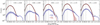Fig. 12.

Distribution of SFGs along Δ log(SSFR)_MS (black solid line). In this illustrative case, we separate the main sequence (red line) and starburst (blue) contribution using $Σ_{SFR}^{\lim} \equiv M d n [Σ_{SFR} (Δ log {(SSFR)}_{MS} = 0.7)]$ $\Sigma_{\mathrm{SFR}}^{\mathrm{lim}}\equiv Mdn[\Sigma_{\mathrm{SFR}}(\Delta\log(\mathrm{SSFR})_{\mathrm{MS}}=0.7)]$ for SFGs with log(M_⋆/M_⊙)> 10.5. The red and blue shaded regions show the scatter (16th and 84th percentiles) introduced by the uncertainties and upper limits of our measurements. The gray region indicates the parameter space where our sample is not complete.

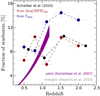Fig. 13.

Redshift evolution of the starburst fraction from the mass-complete sample of radio-selected SFGs used in this work. We adopt two definitions of a starburst galaxy, (a) systems with Δ log(SSFR) > 0.39 and (b) $Σ_{SFR} > Σ_{SFR}^{\lim}$ $\Sigma_{\mathrm{SFR}} > \Sigma_{\mathrm{SFR}}^{\mathrm{lim}}$ (see Sect. 5.1), in both cases log(M_⋆/M_⊙) > 10.5. For comparison, we present the starburst fraction for log(M_⋆/M_⊙) > 10.5 and Δ log(SSFR) > 0.39 UV-/FIR-selected SFGs from Schreiber et al. (2015). The redshift evolution of the observed galaxy pair fraction is shown by the magenta shaded region (Kartaltepe et al. 2007). The gray region shows the major merger fraction predicted by Hopkins et al. (2010).

5.2. Is the centrally concentrated star formation in galaxies evidence of bulge growth?

The finding of compact radio continuum emission of SFGs on and above the MS further support the evidence of star formation enhancement at small radii (e.g., Simpson et al. 2015; Rujopakarn et al. 2016; Nelson et al. 2016a; Fujimoto et al. 2017; Elbaz et al. 2018). Interestingly, while the extent of the stellar component increases with cosmic time, the overall region where most stars are formed remains nearly constant (see Fig. 9). This might indicate that fresh star-forming gas is constantly fueled towards the center of galaxies, either due to VDI, minor or major mergers, and/or tidal interactions (e.g., Larson 2003; Rupke et al. 2010; Sillero et al. 2017; Ellison et al. 2018; Muñoz-Elgueta et al. 2018). Regardless of the dominant mechanism driving the formation of stars in galaxies (on and above the MS), violent and secular galaxy evolutionary channels lead to the formation of a bulge (e.g., Kormendy & Kennicutt 2004; Fisher 2006; Hopkins et al. 2009; Brooks et al. 2016; Tonini et al. 2016). Ultimately, the presence of a dominant bulge could stabilize the gas disk against gravitational instabilities, and thus prevent the formation of stars (e.g., Lang et al. 2014, and references therein).

In this context, we hypothesize that the centrally concentrated star formation activity of most SFGs in the sample might reflect the growth of the bulge, which might precede the quenching of the galaxy from the inside out (e.g., Ellison et al. 2018). At this late evolutionary stage the bulge of massive galaxies is fully quenched, while star formation activity still takes place at large radii (e.g., Tacchella et al. 2015; Rowlands et al. 2018). Spatially resolved studies of low- and high-mass SFGs at high redshift are needed to verify such a scenario, and will allow us to understand how star formation, and hence stellar mass, is distributed in galaxies across cosmic time.

6. Summary

We presented the first systematic study of the radio continuum size evolution of SFGs over 0.35 < z < 2.25. We used a mass-complete sample of 3184 radio-selected SFGs, detected in the VLA COSMOS 3 GHz map (Smolčić et al. 2017a), and performed extensive Monte Carlo simulations to characterize our selection function and validate the robustness of our measurements. We found the following:

The radio continuum size shows no clear dependence on the stellar mass of SFGs with 10.5 ≲ log(M_⋆/M_⊙)≲11.5, which is the mass range where our sample is not affected by our selection function;
MS galaxies are preferentially (but not exclusively) extended, while SFGs above the MS are more compact systems; the median size of SFGs on (above) the MS is R_eff = 1.5 ± 0.2 (1.0 ± 0.2) kpc. Using the parametrization of the form R_eff ∝ (1 + z)^α, we found that the median size remains nearly constant with cosmic time, with α = −0.26 ± 0.08 (0.12 ± 0.14) for SFGs on (above) the MS;
The median radio size of SFGs is smaller (by a factor 1.3−2) than that inferred from optical to UV emission that traces their stellar component (Shibuya et al. 2015). Overall, these results are consistent with compact radio continuum, FIR, and extinction-corrected Hα emission (≲1.5 kpc; e.g., Nelson et al. 2016a; Rujopakarn et al. 2016; Murphy et al. 2017; Cotton et al. 2018; Elbaz et al. 2018; Lindroos et al. 2018);
Most SFGs follow a linear relation in the log(Σ_SFR)−Δ log(SSFR)_MS plane, consistent with previous studies of SFGs in the local Universe (Lutz et al. 2016) and at z ∼ 1 (Magdis et al. 2016). While its normalization increases with redshift, its slope becomes steeper at lower redshifts (from α = 1.5 at z ∼ 2 to 2.6 at z ∼ 0.5);
There is a fraction (≲10%) of MS galaxies harboring starburst-like Σ_SFR, consistent with recent evidence of hidden starbursts within the MS at z ∼ 2 (Elbaz et al. 2018).

Overall, our results suggest that SFGs with enhanced star formation undergo a compaction phase. These systems could be explained in the context of disk instability and/or merger-driven burst of star formation that, depending on the gas content, offset the galaxy from the MS in different proportions (e.g., Fensch et al. 2017; Wang et al. 2019). Since using Δ log(SSFR) alone prevents us from identifying those starburst galaxies hidden within the MS, we recommend using Σ_SFR as well to better identify starbursting systems. Having constraints on Σ_SFR is the first step towards the characterization of the KS relation at high redshift. Exploring in detail the gas content and optical morphology of SFGs in our sample is the subject of an upcoming manuscript.

¹

Not all bins at the bright/compact end exhibit a 100% completeness. We attribute this result to the minimum number of pixels in an island (minpix_isl = 9) used to retrieve the radio sources with PyBDSF. Negative noise fluctuations might hinder the detection of islands of emission above this threshold. Certainly, we verified that using minpix_isl = 6 yields a higher completeness at the bright/compact end. Even so, we adopted minpix_isl = 9 to be consistent with the original VLA COSMOS 3 GHz catalog (Smolčić et al. 2017a).

²

We use this threshold as the number of z ∼ 0.35 starbursts, which is consistent with that derived from the standard Δ log(SSFR)_MS-based definition (see Fig. 13). A different threshold in Σ_SFR also yields a larger starburst fraction at high redshift.

Acknowledgments

E.F.J.A, B.M., A.K, F.B., E.V., E.R.D., K.H., and C.K. acknowledge the support of the Collaborative Research Center 956, subproject A1, funded by the Deutsche Forschungsgemeinschaft (DFG). E.F.J.A. thanks A. Mikler and J. Erler for their encouragement and insightful comments. E.V. acknowledges funding from the DFG grant BE 1837/13-1. P.L. acknowledges funding from the European Research Council (ERC) under the European Union’s Horizon 2020 Research and Innovation Programme (grant agreement No. 694343). S.T. acknowledges support from the ERC Consolidator Grant funding scheme (project ConTExt, grant No. 648179). The Cosmic Dawn Center is funded by the Danish National Research Foundation. J.D. acknowledges the financial assistance of the South African Radio Astronomy Observatory (SARAO; www.ska.ac.za). This work is based on observations with the National Radio Astronomy Observatory, which is a facility of the National Science Foundation operated under cooperative agreement by Associated Universities, Inc., and is also based on data products from observations made with ESO Telescopes at the La Silla Paranal Observatory under ESO program ID 179.A-2005 and on data products produced by TERAPIX and the Cambridge Astronomy Survey Unit on behalf of the UltraVISTA consortium.

References

Alaghband-Zadeh, S., Chapman, S. C., Swinbank, A. M., et al. 2012, MNRAS, 424, 2232 [NASA ADS] [CrossRef] [Google Scholar]
Allen, R. J., Kacprzak, G. G., Glazebrook, K., et al. 2017, ApJ, 834, L11 [NASA ADS] [CrossRef] [Google Scholar]
Anglés-Alcázar, D., Faucher-Giguère, C.-A., Kereš, D., et al. 2017, MNRAS, 470, 4698 [NASA ADS] [CrossRef] [Google Scholar]
Arnouts, S., Moscardini, L., Vanzella, E., et al. 2002, MNRAS, 329, 355 [NASA ADS] [CrossRef] [Google Scholar]
Bell, E. F. 2003, ApJ, 586, 794 [Google Scholar]
Berta, S., Lutz, D., Santini, P., et al. 2013, A&A, 551, A100 [NASA ADS] [CrossRef] [EDP Sciences] [Google Scholar]
Bondi, M., Ciliegi, P., Zamorani, G., et al. 2003, A&A, 403, 857 [NASA ADS] [CrossRef] [EDP Sciences] [Google Scholar]
Bondi, M., Zamorani, G., Ciliegi, P., et al. 2018, A&A, 618, L8 [NASA ADS] [CrossRef] [EDP Sciences] [Google Scholar]
Bouché, N., Cresci, G., Davies, R., et al. 2007, ApJ, 671, 303 [NASA ADS] [CrossRef] [Google Scholar]
Bourke, S., Mooley, K., & Hallinan, G. 2014, ASP Conf. Ser., 485, 367 [NASA ADS] [Google Scholar]
Bouwens, R. J., Illingworth, G. D., Oesch, P., et al. 2012, ApJ, 754, 83 [NASA ADS] [CrossRef] [Google Scholar]
Bremer, M. N., Phillipps, S., Kelvin, L. S., et al. 2018, MNRAS, 476, 12 [NASA ADS] [CrossRef] [Google Scholar]
Brinchmann, J., Charlot, S., White, S. D. M., et al. 2004, MNRAS, 351, 1151 [NASA ADS] [CrossRef] [Google Scholar]
Brooks, A., & Christensen, C. 2016, Astrophys. Space Sci. Lib., 418, 317 [Google Scholar]
Bruzual, G., & Charlot, S. 2003, MNRAS, 344, 1000 [NASA ADS] [CrossRef] [Google Scholar]
Buat, V., Noll, S., Burgarella, D., et al. 2012, A&A, 545, A141 [NASA ADS] [CrossRef] [EDP Sciences] [Google Scholar]
Calabrò, A., Daddi, E., Cassata, P., et al. 2018, ApJ, 862, L22 [NASA ADS] [CrossRef] [Google Scholar]
Capak, P., Aussel, H., Ajiki, M., et al. 2007, ApJS, 172, 99 [NASA ADS] [CrossRef] [Google Scholar]
Casey, C. M., Narayanan, D., & Cooray, A. 2014, Phys. Rev, 541, 45 [Google Scholar]
Chabrier, G. 2003, PASP, 115, 763 [NASA ADS] [CrossRef] [Google Scholar]
Cibinel, A., Daddi, E., Sargent, M. T., et al. 2019, MNRAS, 485, 5631 [NASA ADS] [CrossRef] [Google Scholar]
Condon, J. J. 1992, ARA&A, 30, 575 [NASA ADS] [CrossRef] [MathSciNet] [Google Scholar]
Condon, J. J. 1997, PASP, 109, 166 [NASA ADS] [CrossRef] [Google Scholar]
Coppin, K., Halpern, M., Scott, D., Borys, C., & Chapman, S. 2005, MNRAS, 357, 1022 [NASA ADS] [CrossRef] [Google Scholar]
Cotton, W. D., Condon, J. J., Kellermann, K. I., et al. 2018, ApJ, 856, 67 [NASA ADS] [CrossRef] [Google Scholar]
Da Cunha, E., Charlot, S., & Elbaz, D. 2008, MNRAS, 388, 1595 [NASA ADS] [CrossRef] [Google Scholar]
Daddi, E., Dickinson, M., Morrison, G., et al. 2007, ApJ, 670, 156 [NASA ADS] [CrossRef] [Google Scholar]
Davé, R., Finlator, K., Oppenheimer, B. D., et al. 2010, MNRAS, 404, 1355 [NASA ADS] [Google Scholar]
Decarli, R., Walter, F., Aravena, M., et al. 2016, ApJ, 833, 69 [Google Scholar]
Dekel, A., & Burkert, A. 2014, MNRAS, 438, 1870 [NASA ADS] [CrossRef] [Google Scholar]
Dekel, A., Birnboim, Y., Engel, G., et al. 2009, Nature, 457, 451 [NASA ADS] [CrossRef] [PubMed] [Google Scholar]
Delhaize, J., Smolčić, V., Delvecchio, I., et al. 2017, A&A, 602, A4 [NASA ADS] [CrossRef] [EDP Sciences] [Google Scholar]
Delvecchio, I., Gruppioni, C., Pozzi, F., et al. 2014, MNRAS, 439, 2736 [NASA ADS] [CrossRef] [Google Scholar]
Delvecchio, I., Smolčić, V., Zamorani, G., et al. 2017, A&A, 602, A3 [NASA ADS] [CrossRef] [EDP Sciences] [Google Scholar]
Donley, J. L., Koekemoer, A. M., Brusa, M., et al. 2012, ApJ, 748, 142 [NASA ADS] [CrossRef] [Google Scholar]
Elbaz, D., Daddi, E., Le Borgne, D., et al. 2007, A&A, 468, 33 [NASA ADS] [CrossRef] [EDP Sciences] [Google Scholar]
Elbaz, D., Dickinson, M., Hwang, H. S., et al. 2011, A&A, 533, A119 [NASA ADS] [CrossRef] [EDP Sciences] [Google Scholar]
Elbaz, D., Leiton, R., Nagar, N., et al. 2018, A&A, 616, A110 [NASA ADS] [CrossRef] [EDP Sciences] [Google Scholar]
Ellison, S. L., Sánchez, S. F., Ibarra-Medel, H., et al. 2018, MNRAS, 474, 2039 [NASA ADS] [CrossRef] [Google Scholar]
Feng, Y., Matteo, T. D., Croft, R., et al. 2015, ApJ, 808, L17 [NASA ADS] [CrossRef] [Google Scholar]
Fensch, J., Renaud, F., Bournaud, F., et al. 2017, MNRAS, 465, 1934 [NASA ADS] [CrossRef] [Google Scholar]
Fisher, D. B. 2006, ApJ, 642, L17 [NASA ADS] [CrossRef] [Google Scholar]
Fujimoto, S., Ouchi, M., Shibuya, T., & Nagai, H. 2017, ApJ, 850, 83 [NASA ADS] [CrossRef] [Google Scholar]
Furlong, M., Bower, R. G., Crain, R. A., et al. 2017, MNRAS, 465, 722 [NASA ADS] [CrossRef] [Google Scholar]
Garn, T., Green, D. A., Riley, J. M., & Alexander, P. 2009, MNRAS, 397, 1101 [NASA ADS] [CrossRef] [Google Scholar]
Genzel, R., Tacconi, L. J., Gracia-Carpio, J., et al. 2010, MNRAS, 407, 2091 [NASA ADS] [CrossRef] [Google Scholar]
Genzel, R., Tacconi, L. J., Lutz, D., et al. 2015, ApJ, 800, 20 [NASA ADS] [CrossRef] [Google Scholar]
Gómez-Guijarro, C., Toft, S., Karim, A., et al. 2018, ApJ, 856, 121 [NASA ADS] [CrossRef] [Google Scholar]
González, V., Labbé, I., Bouwens, R. J., et al. 2010, ApJ, 713, 115 [NASA ADS] [CrossRef] [Google Scholar]
González, V., Bouwens, R., Illingworth, G., et al. 2014, ApJ, 781, 34 [NASA ADS] [CrossRef] [Google Scholar]
Guidetti, D., Bondi, M., Prandoni, I., et al. 2017, MNRAS, 471, 210 [NASA ADS] [CrossRef] [Google Scholar]
Hales, C. A., Murphy, T., Curran, J. R., et al. 2012, MNRAS, 425, 979 [NASA ADS] [CrossRef] [Google Scholar]
Hayward, C. C., Kereš, D., Jonsson, P., et al. 2011, ApJ, 743, 159 [CrossRef] [Google Scholar]
Helou, G., & Bicay, M. D. 1993, ApJ, 415, 93 [NASA ADS] [CrossRef] [Google Scholar]
Helou, G., Soifer, B. T., & Rowan-Robinson, M. 1985, ApJ, 298, 7 [Google Scholar]
Hodge, J. A., Carilli, C. L., Walter, F., et al. 2012, ApJ, 760, 11 [Google Scholar]
Hodge, J. A., Swinbank, A. M., Simpson, J. M., et al. 2016, ApJ, 833, 103 [Google Scholar]
Hogg, D. W., & Turner, E. L. 1998, PASP, 110, 727 [NASA ADS] [CrossRef] [Google Scholar]
Hopkins, P. F., Cox, T. J., Younger, J. D., & Hernquist, L. 2009, ApJ, 691, 1168 [Google Scholar]
Hopkins, P. F., Croton, D., Bundy, K., et al. 2010, ApJ, 724, 915 [NASA ADS] [CrossRef] [Google Scholar]
Ilbert, O., Arnouts, S., McCracken, H. J., et al. 2006, A&A, 457, 841 [NASA ADS] [CrossRef] [EDP Sciences] [Google Scholar]
Ilbert, O., Salvato, M., Floc’h, E. L., et al. 2010, ApJ, 709, 644 [NASA ADS] [CrossRef] [Google Scholar]
Kaplan, E. L., & Meier, P. 1958, J. Am. Stat. Assoc., 53, 457 [Google Scholar]
Karim, A., Schinnerer, E., Martínez-Sansigre, A., et al. 2011, ApJ, 730, 61 [NASA ADS] [CrossRef] [Google Scholar]
Kartaltepe, J. S., Sanders, D. B., Scoville, N. Z., et al. 2007, ApJS, 172, 320 [NASA ADS] [CrossRef] [Google Scholar]
Kartaltepe, J. S., Dickinson, M., Alexander, D. M., et al. 2012, ApJ, 757, 23 [CrossRef] [Google Scholar]
Kennicutt, J. R. C. 1998, ARA&A, 36, 189 [Google Scholar]
Kennicutt, R. C., & Evans, N. J. 2011, ARA&A, 50, 531 [Google Scholar]
Kereš, D., Katz, N., Fardal, M., Davé, R., & Weinberg, D. H. 2009, MNRAS, 395, 160 [NASA ADS] [CrossRef] [Google Scholar]
Khochfar, S., & Silk, J. 2006, ApJ, 648, L21 [NASA ADS] [CrossRef] [Google Scholar]
Khochfar, S., & Silk, J. 2009, MNRAS, 397, 506 [NASA ADS] [CrossRef] [Google Scholar]
Kobayashi, T., Komori, Y., Yoshida, K., & Nishimura, J. 2004, ApJ, 601, 340 [NASA ADS] [CrossRef] [Google Scholar]
Kormendy, J., & Kennicutt, R. C. 2004, ARA&A, 42, 603 [NASA ADS] [CrossRef] [Google Scholar]
Laigle, C., McCracken, H. J., Ilbert, O., et al. 2016, ApJS, 224, 24 [NASA ADS] [CrossRef] [Google Scholar]
Lang, P., Wuyts, S., Somerville, R. S., et al. 2014, ApJ, 788, 11 [NASA ADS] [CrossRef] [Google Scholar]
Larson, R. 2003, in Mass-Transfer Induced Activity in Galaxies, ed. I. Shlosman (Cambridge: Cambridge University Press) [Google Scholar]
Leslie, S., Sargent, M. T., Schinnerer, E., et al. 2018, A&A, 615, A7 [NASA ADS] [CrossRef] [EDP Sciences] [Google Scholar]
Lindroos, L., Knudsen, K. K., Stanley, F., et al. 2018, MNRAS, 476, 3544 [NASA ADS] [CrossRef] [Google Scholar]
Lutz, D., Berta, S., Contursi, A., et al. 2016, A&A, 591, A136 [NASA ADS] [CrossRef] [EDP Sciences] [Google Scholar]
Magdis, G. E., Rigopoulou, D., Huang, J. S., & Fazio, G. G. 2010, MNRAS, 401, 1521 [NASA ADS] [CrossRef] [Google Scholar]
Magdis, G. E., Bureau, M., Stott, J. P., et al. 2016, MNRAS, 456, 4533 [NASA ADS] [CrossRef] [Google Scholar]
Magnelli, B., Lutz, D., Saintonge, A., et al. 2014, A&A, 561, A86 [NASA ADS] [CrossRef] [EDP Sciences] [Google Scholar]
Magnelli, B., Ivison, R. J., Lutz, D., et al. 2015, A&A, 573, A45 [NASA ADS] [CrossRef] [EDP Sciences] [Google Scholar]
McCracken, H. J., Milvang-Jensen, B., Dunlop, J., et al. 2012, A&A, 544, A156 [NASA ADS] [CrossRef] [EDP Sciences] [Google Scholar]
Miettinen, O., Delvecchio, I., Smolčić, V., et al. 2017, A&A, 597, A5 [NASA ADS] [CrossRef] [EDP Sciences] [Google Scholar]
Mitra, S., Davé, R., Simha, V., & Finlator, K. 2017, MNRAS, 464, 2766 [NASA ADS] [CrossRef] [Google Scholar]
Miyazaki, S., Komiyama, Y., Nakaya, H., et al. 2012, Proc. SPIE, 8446, 84460Z [NASA ADS] [CrossRef] [Google Scholar]
Mohan, N., & Rafferty, D. 2015, Astrophysics Source Code Library [record ascl:1502.007] [Google Scholar]
Möllenhoff, C., Popescu, C. C., & Tuffs, R. J. 2006, A&A, 456, 941 [NASA ADS] [CrossRef] [EDP Sciences] [Google Scholar]
Moreno, J., Torrey, P., Ellison, S. L., et al. 2015, MNRAS, 448, 1107 [NASA ADS] [CrossRef] [Google Scholar]
Mowla, L., van Dokkum, P., Brammer, G., et al. 2018, ApJ, submitted [arXiv:1808.04379] [Google Scholar]
Muñoz-Elgueta, N., Torres-Flores, S., Amram, P., et al. 2018, MNRAS, 480, 3257 [NASA ADS] [CrossRef] [Google Scholar]
Murphy, E. J. 2009, ApJ, 706, 482 [NASA ADS] [CrossRef] [Google Scholar]
Murphy, E. J., Braun, R., Helou, G., et al. 2006a, ApJ, 638, 157 [NASA ADS] [CrossRef] [Google Scholar]
Murphy, E. J., Helou, G., Braun, R., et al. 2006b, ApJ, 651, L111 [NASA ADS] [CrossRef] [Google Scholar]
Murphy, E. J., Bremseth, J., Mason, B. S., et al. 2012, ApJ, 761, 97 [NASA ADS] [CrossRef] [Google Scholar]
Murphy, E. J., Momjian, E., Condon, J. J., et al. 2017, ApJ, 839, 35 [NASA ADS] [CrossRef] [Google Scholar]
Narayanan, D., Hayward, C. C., Cox, T. J., et al. 2010, MNRAS, 401, 1613 [NASA ADS] [CrossRef] [MathSciNet] [Google Scholar]
Nelson, E. J., van Dokkum, P. G., Brammer, G., et al. 2012, ApJ, 747, L28 [NASA ADS] [CrossRef] [Google Scholar]
Nelson, E. J., van Dokkum, P. G., Momcheva, I. G., et al. 2016a, ApJ, 817, L9 [NASA ADS] [CrossRef] [Google Scholar]
Nelson, E. J., van Dokkum, P. G., Schreiber, N. M. F., et al. 2016b, ApJ, 828, 27 [NASA ADS] [CrossRef] [Google Scholar]
Noeske, K. G., Weiner, B. J., Faber, S. M., et al. 2007, ApJ, 660, L43 [Google Scholar]
Oser, L., Ostriker, J. P., Naab, T., Johansson, P. H., & Burkert, A. 2010, ApJ, 725, 2312 [NASA ADS] [CrossRef] [Google Scholar]
Pannella, M., Carilli, C. L., Daddi, E., et al. 2009, ApJ, 698, L116 [Google Scholar]
Pannella, M., Elbaz, D., Daddi, E., et al. 2015, ApJ, 807, 141 [NASA ADS] [CrossRef] [Google Scholar]
Pearson, W. J., Wang, L., Hurley, P. D., et al. 2018, A&A, 615, A146 [NASA ADS] [CrossRef] [EDP Sciences] [Google Scholar]
Peng, Y.-J., Lilly, S. J., Kovač, K., et al. 2010, ApJ, 721, 193 [NASA ADS] [CrossRef] [Google Scholar]
Polletta, M., Tajer, M., Maraschi, L., et al. 2007, ApJ, 663, 81 [NASA ADS] [CrossRef] [Google Scholar]
Renzini, A., & Peng, Y.-J. 2015, ApJ, 801, L29 [NASA ADS] [CrossRef] [Google Scholar]
Richards, E. A. 2000, ApJ, 533, 611 [NASA ADS] [CrossRef] [Google Scholar]
Riechers, D. A., Bradford, C. M., Clements, D. L., et al. 2013, Nature, 496, 329 [Google Scholar]
Riechers, D. A., Carilli, C. L., Capak, P. L., et al. 2014, ApJ, 796, 84 [NASA ADS] [CrossRef] [Google Scholar]
Rodighiero, G., Daddi, E., Baronchelli, I., et al. 2011, ApJ, 739, L40 [NASA ADS] [CrossRef] [Google Scholar]
Rodighiero, G., Renzini, A., Daddi, E., et al. 2014, MNRAS, 443, 19 [NASA ADS] [CrossRef] [Google Scholar]
Romano-Díaz, E., Shlosman, I., Choi, J.-H., & Sadoun, R. 2014, ApJ, 790, L32 [NASA ADS] [CrossRef] [Google Scholar]
Romano-Díaz, E., Garaldi, E., Borzyszkowski, M., & Porciani, C. 2017, MNRAS, 469, 1809 [NASA ADS] [CrossRef] [Google Scholar]
Rowlands, K., Heckman, T., Wild, V., et al. 2018, MNRAS, 480, 2544 [NASA ADS] [CrossRef] [Google Scholar]
Rujopakarn, W., Dunlop, J. S., Rieke, G. H., et al. 2016, ApJ, 833, 12 [NASA ADS] [CrossRef] [Google Scholar]
Rupke, D. S. N., Kewley, L. J., & Barnes, J. E. 2010, ApJ, 710, L156 [NASA ADS] [CrossRef] [Google Scholar]
Salim, S., Rich, R. M., Charlot, S., et al. 2007, ApJS, 173, 267 [NASA ADS] [CrossRef] [Google Scholar]
Salmon, B., Papovich, C., Finkelstein, S. L., et al. 2015, ApJ, 799, 183 [NASA ADS] [CrossRef] [Google Scholar]
Sanders, D. B., Salvato, M., Aussel, H., et al. 2007, ApJS, 172, 86 [Google Scholar]
Sargent, M. T., Schinnerer, E., Murphy, E., et al. 2010, ApJS, 186, 341 [NASA ADS] [CrossRef] [Google Scholar]
Sargent, M. T., Béthermin, M., Daddi, E., & Elbaz, D. 2012, ApJ, 747, L31 [NASA ADS] [CrossRef] [Google Scholar]
Schinnerer, E., Groves, B., Sargent, M. T., et al. 2016, ApJ, 833, 112 [NASA ADS] [CrossRef] [Google Scholar]
Schreiber, C., Pannella, M., Elbaz, D., et al. 2015, A&A, 575, A74 [NASA ADS] [CrossRef] [EDP Sciences] [Google Scholar]
Schreiber, C., Pannella, M., Leiton, R., et al. 2017, A&A, 599, A134 [NASA ADS] [CrossRef] [EDP Sciences] [Google Scholar]
Sellwood, J. A. 2014, Rev. Mod. Phys., 86, 1 [NASA ADS] [CrossRef] [Google Scholar]
Shibuya, T., Ouchi, M., & Harikane, Y. 2015, ApJS, 219, 15 [NASA ADS] [CrossRef] [Google Scholar]
Sillero, E., Tissera, P. B., Lambas, D. G., & Michel-Dansac, L. 2017, MNRAS, 472, 4404 [NASA ADS] [CrossRef] [Google Scholar]
Simpson, J. M., Smail, I., Swinbank, A. M., et al. 2015, ApJ, 799, 81 [CrossRef] [Google Scholar]
Smolčić, V., Novak, M., Bondi, M., et al. 2017a, A&A, 602, A1 [NASA ADS] [CrossRef] [EDP Sciences] [Google Scholar]
Smolčić, V., Delvecchio, I., Zamorani, G., et al. 2017b, A&A, 602, A2 [NASA ADS] [CrossRef] [EDP Sciences] [Google Scholar]
Speagle, J. S., Steinhardt, C. L., Capak, P. L., & Silverman, J. D. 2014, ApJS, 214, 15 [NASA ADS] [CrossRef] [Google Scholar]
Stark, D. P., Schenker, M. A., Ellis, R., et al. 2013, ApJ, 763, 129 [NASA ADS] [CrossRef] [Google Scholar]
Steinhardt, C. L., Speagle, J. S., Capak, P., et al. 2014, ApJ, 791, L25 [Google Scholar]
Szokoly, G. P., Bergeron, J., Hasinger, G., et al. 2004, ApJS, 155, 271 [NASA ADS] [CrossRef] [Google Scholar]
Tacchella, S., Carollo, C. M., Renzini, A., et al. 2015, Science, 348, 314 [NASA ADS] [CrossRef] [Google Scholar]
Tacchella, S., Dekel, A., Carollo, C. M., et al. 2016, MNRAS, 457, 2790 [NASA ADS] [CrossRef] [Google Scholar]
Tacconi, L. J., Neri, R., Genzel, R., et al. 2013, ApJ, 768, 74 [Google Scholar]
Tacconi, L. J., Genzel, R., Saintonge, A., et al. 2018, ApJ, 853, 179 [NASA ADS] [CrossRef] [Google Scholar]
Tonini, C., Mutch, S. J., Croton, D. J., & Wyithe, J. S. B. 2016, MNRAS, 459, 4109 [NASA ADS] [CrossRef] [Google Scholar]
van der Wel, A., Franx, M., van Dokkum, P. G., et al. 2014, ApJ, 788, 28 [NASA ADS] [CrossRef] [Google Scholar]
Walter, F., Riechers, D., Cox, P., et al. 2009, Nature, 457, 699 [NASA ADS] [CrossRef] [PubMed] [Google Scholar]
Wang, L., De Lucia, G., Fontanot, F., & Hirschmann, M. 2019, MNRAS, 482, 4454 [NASA ADS] [CrossRef] [Google Scholar]
Wellons, S., Torrey, P., Ma, C.-P., et al. 2015, MNRAS, 449, 361 [NASA ADS] [CrossRef] [Google Scholar]
Whitaker, K. E., van Dokkum, P. G., Brammer, G., & Franx, M. 2012, ApJ, 754, L29 [NASA ADS] [CrossRef] [Google Scholar]
Whitaker, K. E., Franx, M., Leja, J., et al. 2014, ApJ, 795, 104 [NASA ADS] [CrossRef] [MathSciNet] [Google Scholar]
Windhorst, R. A., Mathis, D., & Neuschaefer, L. 1990, in Evolution of the Universe of Galaxies, ASP Conf. Ser., 10, 389 [NASA ADS] [Google Scholar]
Wuyts, S., Schreiber, N. M. F., van der Wel, A., et al. 2011, ApJ, 742, 96 [NASA ADS] [CrossRef] [Google Scholar]
Yun, M. S., Reddy, N. A., & Condon, J. J. 2001, ApJ, 554, 803 [NASA ADS] [CrossRef] [Google Scholar]

Appendix A: Flux boosting

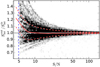Fig. A.1.

Flux boosting for unresolved sources as a function of S/N estimated from MC simulations. The solid and dashed red lines show the 50th percentile, and the 14th and 84th percentiles of the distribution as a function of S/N. The vertical blue dashed line indicates our detection threshold (S/N = 5).

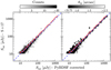Fig. A.2.

Comparison between the flux density of 3184 SFGs in the sample (resolved and unresolved) derived from PyBDSF (corrected) and those reported by Smolčić et al. (2017a). The solid and dashed red lines show the 50th percentile, and 14th and 84th percentiles of the distribution as a function of the flux density reported in this study.

Appendix B: Size evolution of SFGs using uncorrected FWHM and flux density

The extensive Monte Carlo simulations performed in this work indicate that the FWHM and flux density are being overestimated for most of the radio sources in the sample (see Fig. 5). Using these values, however, does not systematically affect the trends and relations presented in this work, as initially inferred from Fig. B.1. First, this approach also leads to a flat relation between the median radio size and stellar mass of SFGs (Fig. B.2). Second, we find a similar radio size and Σ_SFR dichotomy between SFGs on and above the MS (Figs. B.1 and B.3). Using uncorrected measurements leads to a smaller fraction of MS galaxies with starburst-like Σ_SFR (Fig. B.4), given that the size of faint MS galaxies is overestimated and, consequently, Σ_SFR becomes smaller. We note that regardless of the use of corrected or uncorrected values, the fraction of starburst-like Σ_SFR systems remains unclear, due to the presence of MS galaxies that are unresolved in the VLA COSMOS 3 GHz map.

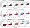Fig. B.1.

Upper panels: sample of 3184 SFGs in the SFR−M_⋆−z plane color-coded for the number of sources per bin. Solid and dashed black lines show the position of the MS of SFGs and the associated dispersion given by Schreiber et al. (2015). Vertical red solid lines show the mass-limit above which we consistently probe SFGs on and above the MS. Middle and lower panels: median size and star formation surface density, respectively, of the 3184 SFGs in the sample. We use 1000 MC realizations to include the values for unresolved sources, which are drawn from the distributions described in Sects. 4.2 and 4.4.

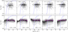Fig. B.2.

Sample of 3184 SFGs in the R_eff−M_⋆−z plane. The blue solid line shows the maximum size, corresponding to the 10% completeness level, that can be observed for a galaxy with Δ log(SSFR) = 0 evaluated at the central redshift value per bin. Blue dashed lines show the mass-limit above which we consistently probe SFGs on and above the MS. Black arrows show the upper limits for the size of unresolved sources. Lower panels: density distribution per stellar mass bin (0.5 dex width) of SFGs in the R_eff−M_⋆−z plane. Contour levels are at the 10, 20, 30, 40, 50, 60, 70, 80, and 90th percentiles. The median size derived via the KM estimator is shown by the dark magenta circles; the error bars correspond to the 16th and 86th percentiles of the distribution.

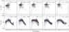Fig. B.3.

Upper panels: star-forming galaxies with $M_{⋆} > M_{⋆}^{lim}$ $M_\star > M_\star^{\rm lim}$ in the size−Δ log(SSFR)−z plane. The blue solid line shows the maximum size, corresponding to the 10% completeness level, that can be observed for a galaxy with $M_{⋆} = M_{⋆}^{lim}$ $M_\star=M_\star^{\rm lim}$ evaluated at the central redshift value per bin. Black arrows show the upper limits for the size of unresolved sources. Lower panels: density distribution per Δ log(SSFR) bin (0.5 dex width) of SFGs in the size−Δ log(SSFR)−z plane. Contour levels are at the 10, 20, 30, 40, 50, 60, 70, 80, and 90th percentiles. The median size derived via the KM estimator is shown by the dark magenta circles; the error bars correspond to the 16th and 86th percentiles of the distribution.

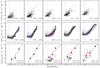Fig. B.4.

Upper panels: star-forming galaxies with $M_{⋆} > M_{⋆}^{lim}$ $M_\star > M_\star^{\rm lim}$ in the Σ_SFR−Δ log(SSFR)−z plane. Dashed blue lines show the Δ log(SSFR) limit of −0.3 above which our sample of SFGs is complete in terms of distance to the MS. Black arrows show the lower limits for the size of unresolved sources. Middle panels: density distribution per Δ log(SSFR) bin (0.4 dex width) of SFGs in the Σ_SFR−Δ log(SSFR)−z plane. Contour levels are at the 10, 20, 30, 40, 50, 60, 70, 80, and 90th percentiles. The median size derived via the KM estimator is shown by the dark magenta circles; the error bars correspond to the 16th and 86th percentiles of the distribution. Lower panels: power law describing the Σ_SFR−Δ log(SSFR) relation (dotted black line). The slope and normalization are given in the lower right corner. The median size derived via the KM estimator is also shown by the dark magenta circles. For comparison, we present the compilation of SFGs from Genzel et al. (2010, black filled circles), Tacconi et al. (2013, black empty squares), Elbaz et al. (2018, red pentagons), and Lang et al. (in prep., orange triangles). Black arrow illustrates the factor to be considered when comparing Σ_SFR of galaxies in our sample with that reported by Genzel et al. (2010) and Tacconi et al. (2013).

Appendix C: Tables

Table C.1.

Radio continuum size as a function of the stellar mass of SFGs.

Table C.2.

Radio continuum size as a function of distance to the MS of SFGs.

Table C.3.

Star formation surface density (Σ_SFR) as a function of distance to the MS of SFGs.

All Tables