| Issue |
A&A
Volume 625, May 2019
|
|
|---|---|---|
| Article Number | A17 | |
| Number of page(s) | 23 | |
| Section | Planets and planetary systems | |
| DOI | https://doi.org/10.1051/0004-6361/201935019 | |
| Published online | 01 May 2019 | |
The SOPHIE search for northern extrasolar planets
XIV. A temperate (Teq ~ 300 K) super-earth around the nearby star Gliese 411★,★★
1
Facultad de Ciencias Exactas y Naturales, Universidad de Buenos Aires,
Buenos Aires, Argentina
e-mail: rodrigo.diaz@unige.ch
2
CONICET – Universidad de Buenos Aires, Instituto de Astronomía y Física del Espacio (IAFE),
Buenos Aires, Argentina
3
CNRS, IPAG, Université Grenoble Alpes,
38000
Grenoble, France
4
CNRS, Aix-Marseille Université, CNES,
LAM,
Marseille, France
5
Departamento de Astronomía, Universidad de Concepción,
Casilla 160-C,
Concepción, Chile
6
Center of Excellence in Information Systems, Tennessee State University,
Nashville,
TN 37209, USA
7
Observatoire de Haute Provence, CNRS, Aix-Marseille Université, Institut Pythéas UMS 3470,
04870
Saint-Michel-l’Observatoire, France
8
Observatoire Astronomique de l’Université de Genève,
51 Chemin des Maillettes,
1290
Versoix, Switzerland
9
Institut d’Astrophysique de Paris, UMR7095 CNRS, Université Pierre & Marie Curie,
98bis boulevard Arago,
75014
Paris, France
10
Instituto de Astrofísica e Ciências do Espaço, Universidade do Porto, CAUP, Rua das Estrelas,
4150-762
Porto, Portugal
11
Departamento de Física e Astronomia, Faculdade de Ciências, Universidade do Porto, Rua do Campo Alegre,
4169-007
Porto, Portugal
12
Canada-France-Hawaii Telescope Corporation,
65-1238 Mamalahoa Hwy,
Kamuela,
HI 96743, USA
13
Department of Physics, University of Warwick,
Coventry CV4 7AL, UK
14
Centre for Exoplanets and Habitability, University of Warwick,
Coventry CV4 7AL, UK
Received:
4
January
2019
Accepted:
13
February
2019
Periodic radial velocity variations in the nearby M-dwarf star Gl 411 are reported, based on measurements with the SOPHIE spectrograph. Current data do not allow us to distinguish between a 12.95-day period and its one-day alias at 1.08 days, but favour the former slightly. The velocity variation has an amplitude of 1.6 m s−1, making this the lowest-amplitude signal detected with SOPHIE up to now. We have performed a detailed analysis of the significance of the signal and its origin, including extensive simulations with both uncorrelated and correlated noise, representing the signal induced by stellar activity. The signal is significantly detected, and the results from all tests point to its planetary origin. Additionally, the presence of an additional acceleration in the velocity time series is suggested by the current data. On the other hand, a previously reported signal with a period of 9.9 days, detected in HIRES velocities of this star, is not recovered in the SOPHIE data. An independent analysis of the HIRES dataset also fails to unveil the 9.9-day signal. If the 12.95-day period is the real one, the amplitude of the signal detected with SOPHIE implies the presence of a planet, called Gl 411 b, with a minimum mass of around three Earth masses, orbiting its star at a distance of 0.079 AU. The planet receives about 3.5 times the insolation received by Earth, which implies an equilibrium temperature between 256 and 350 K, and makes it too hot to be in the habitable zone. At a distance of only 2.5 pc, Gl 411 b, is the third closest low-mass planet detected to date. Its proximity to Earth will permit probing its atmosphere with a combination of high-contrast imaging and high-dispersion spectroscopy in the next decade.
Key words: planetary systems / techniques: radial velocities / stars: low-mass / stars: individual: Gl 411
Full Table 2 is only available at the CDS via anonymous ftp to cdsarc.u-strasbg.fr (130.79.128.5) or via http://cdsarc.u-strasbg.fr/viz-bin/qcat?J/A+A/625/A17
© ESO 2019
1 Introduction
It is usually stated that low-mass stars are prime targets for extrasolar planet searches. Their relative low masses and small radii permit detecting smaller planets than on their hotter counterparts. M dwarfs also present the advantage that planets orbiting in the habitable zone are much easier to detect, because in addition to the advantages due to their masses and radii, the habitable zone lies much closer to the star than in solar-type stars. In addition, the atmospheres of planets transiting close M dwarfs could be amenable to characterisation in the coming decade by the James Webb Space Telescope (Doyon et al. 2014; Beichman et al. 2014), or on the ground with stabilised high-resolution spectrographs on medium to large-size telescopes (e.g. Snellen et al. 2008; Wyttenbach et al. 2017; Allart et al. 2018). Another favourable aspect is that the majority of the closest neighbours to the solar system are low-mass stars. This opens the possibility of the characterisation of the atmospheres of non-transiting planets around low-mass stars by a combination of high-dispersion spectroscopy and high contrast imaging (Sparks & Ford 2002; Snellen et al. 2015). These observations will be plausible with the next-generation large-aperture telescopes, such as the E-ELT, but even with the current instrumentation, this is possible for the most favourable cases (Lovis et al. 2017). Similar planets around solar type stars will only be accessible for characterisation with highly ambitious space missions, which will not be in operation before the middle of the century.
Besides theoretical advantages, recent results show that rocky planets orbiting low-mass stars are abundant: based on results from the HARPS velocity survey, Bonfils et al. (2013) reported an occurrence rate above 50% for super-Earth planets on orbits with periods between 10 and 100 days; using Kepler photometry Dressing & Charbonneau (2015) reported an average of 2.5 planets with radii between one and four Earth radii per M-star host, on orbits with periods shorter than 200 days; Gaidos et al. (2016) concluded that M stars host an average of 2.2 planets per star with periods between 1.5 and 180 days. Furthermore, planets orbiting in the habitable zone of low-mass stars are also relatively common. Dressing & Charbonneau (2015) reported an average between 0.16–0.24 Earth-sized planets in the habitable zone of M dwarfs, based on Kepler photometry. Bonfils et al. (2013) reported a fraction  , although this number is probably slightly overestimated, as it included a planet candidate later shown to be likely produced by activity (Robertson et al. 2014).
The SOPHIE search for northern extrasolar planets is a radial velocity survey operating since 2006 (Bouchy et al. 2009a), and is divided in a number of sub-programmes, each targeting different stars and/or planets. In particular, the sub-programme three (SP3) is dedicated to finding planets around low-mass stars. A sample of relatively bright northern M-dwarf stars is observed systematically in order to constrain the presence of planets and also to find targets amenable to detailed characterisation, either now or using future observing facilities.
Gl 411 is one of the brightest M-dwarf stars in the sky (Lépine & Gaidos 2011; Gaidos et al. 2014). As such, it has been intensively observed formany years. In a number of opportunities, detections of orbiting companions were reported, starting with the astrometric study by van de Kamp & Lippincott (1951), who reported a 1.14-yr period object on an eccentric orbit, with a minimum mass as low as 0.03 M⊙. The result was later revised by Lippincott (1960), who concluded that the orbiting companion is on an eigth-year orbit, with a mass as low as 0.01 M⊙, that is around ten Jupiter masses. More recently, Gatewood (1996) reported the detection of an astrometric signal with a period of 5.8 yr, which implies a companion mass as low as 0.9 MJup. These detections remain unconfirmed to this day, as far as we are aware. Using radial velocity observations from the HIRES spectrograph, Butler et al. (2017) recently reported the presence of a periodic signal with a period of 9.9 days, and an amplitude compatible with a planetary companion with a minimum mass of 3.8 M⊕.
In this article, we report the detection of a 3-Earth-minimum-mass companion on a 12.95-day period orbit around the nearby star Gl 411 (Lalande 21185, HD 95735), based on almost seven years of measurements from the SOPHIE SP3. Interestingly, Gl 411 was initially chosen as a possible SOPHIE standard star because of its brightness and of its reported relative low variability level of 10 m s−1 (Butler et al. 2004). Before the upgrade of SOPHIE in 2011 (see Sect. 3), the low velocity scatter was confirmed and therefore Gl 411 was continued to be observed as a standard star. The low velocity rms was further confirmed during our first season of observation with the upgraded instrument. The consequently large number of measurements obtained on this target finally revealed a periodic 1.6-m s−1 variation with a period of around 12.95 days.
In Sect. 2 of this article, the stellar parameters of Gl 411 are presented, possible values of the rotational period of the star are discussed, and the detection of the rotational modulation using photometric ground-based observations is described. In Sect. 3 we present the spectroscopic observations as well as the measurement of the radial velocities and ancillary observables. In Sect. 4 the physical and probability model used to describe the data is presented, and the analysis of the data is described. The detection of a periodic signal, together with the validation of its planetary origin, are also presented here. In Sect. 5 we present a few discussions on the planetary companion detected, and the analysis of the HIRES data. In particular, in Sect. 5.2 we show that the 9.9-day period signal announced by Butler et al. (2017) is not found in the SOPHIE data, and that an independent analysis of the HIRES velocity also fails to recover the reported signal. In Sect. 6 we present some brief conclusions.
2 Stellar characterisation
The star Gl 411 is an early M dwarf (M1.9; Mann et al. 2015) located in the constellation of Ursa Major. It is the sixth star from the Sun, after the three-star Alpha Centauri system, Barnard’s star, and CN Leonis (van Altena et al. 1995). With apparent visual magnitude of 7.5 (J = 4.2; Cutri et al. 2003), it is one of the brightest M-dwarf stars in the sky (Lépine & Gaidos 2011; Gaidos et al. 2014). The stellar parameters were determined by Mann et al. (2015) and are listed in Table 1. The mass was computed by these authors using the mass-luminosity relation by Delfosse et al. (2000) and the radius was obtained from the Teff and the bolometric flux, the latter estimated from optical and near-infrared flux-calibrated spectra, and the former from comparing the spectra to the BT-SETTL atmosphere models (Allard et al. 2012, 2013).
The X-ray flux of Gl 411 was measured by the XMM-Newton satellite (Jansen et al. 2001) and presented in the third XMM-Newton serendipitous source catalogue (Rosen et al. 2016). The value of the flux measured in 2001 (Fx = (6.59 ± 0.13) × 10−13 erg cm−2 s−1), according to the DR8 of the catalogue implies Rx = Lx∕Lbol = (6.09 ± 0.13) × 10−6, using the bolometric flux from Mann et al. (2015), and where the uncertainties were obtained by propagating the errors in the X-ray count rate, the bolometric flux and the stellar parallax, assuming normal errors in all cases.
Regarding the rotational velocity and period, Delfosse et al. (1998) reported an upper limit for the velocity, vsini⋆ < 2.9 km s−1. Using SOPHIE spectra, Houdebine (2010) measured it to be vsin i⋆ = 0.61 km s−1, with a general uncertainty of 0.3 km s−1. However, this value is at the limit of their detection sensitivity. Using a value of the stellar radius based on V-band photometry, they measured a rotational period, P∕sini⋆ = 36.4 d. With theradius determination from Mann et al. (2015), the rotational period is P∕ sini⋆ = 32.3 d. These determinations based on the vsini⋆ suffer from a relative uncertainty of around 51%, if a 10% uncertainty on the stellar radius is assumed.
On the other hand, the rotation-activity calibration for low-mass stars of Astudillo-Defru et al. (2017a) indicates a rotational period Prot = 91 ± 18 days, roughly twice the value reported by Noyes et al. (1984), for the measured value of the activity index,  = − 5.51 ± 0.13. The activity-rotation calibration based on X-ray luminosity by Kiraga & Stepien (2007) produces a rotational period of 72.5 ± 8.4 days for the XMM-Newton X-ray flux, and using the “low mass” calibration, obtained using stars with masses between 0.33 M⊙ and 0.39 M⊙. Gl 411 is close to the upperbound of the calibration stars, and therefore the “medium mass” calibration of Kiraga & Stepien (2007), using stars with masses between 0.43 M⊙ and 0.52 M⊙, may also be considered. The medium-mass calibration produces a rotational period of 57 ± 12 days.
Finally, Noyes et al. (1984) reported the rotational period to be 48 days, based on modulation detected in the S-index measured by the H-K programme (Vaughan et al. 1978). This value implies a rotational velocity between v = 0.41−0.46 km s−1, depending on the adopted stellar radius. Because of the large uncertainties in rotational velocity and those associated with the activity calibrations, these values of rotational period are formally in agreement with each other (differences below 3 σ).
Stellar parameters of Gl 411.
Photometric observations
The stellar rotational period is a key element in the validation of the planetary nature of periodic signals detected in RV. To measure a precise rotational period, we analysed photometric observations of Gl 411 acquired contemporaneously with our SOPHIE radial-velocity measurements during the 2011 through 2018 observing seasons with the Tennessee State University (TSU) T3 0.40 m automatic photoelectric telescope (APT) at Fairborn Observatory in southern Arizona. Details on the instrument, observing strategy, and data analysis are given in Appendix B.
A frequency spectrum, computed as the reduction in total variance of the data versus trial frequency, was performed on the V and B data from each of the eight observing seasons. The frequency analyses spanned a frequency range of 0.005–0.95 cycles day−1 (c d−1), corresponding to a period-search range of 1–200 days. The results of our analysis of the photometric data are summarized in Table B.1. The resulting periods and peak-to-peak amplitudes are given in Cols. 6 and 7. Periodic variations were found in seven of the eight observing seasons, at least for the B data sets. The weighted mean of the 12 detected periods is 56.15 ± 0.27 days. The peak-to-peak amplitudes ranged between 0.002 and 0.008 mag. We take the 56.15-day period to be the stellar rotation period revealed by rotational modulation in the visibility of small star spots on the stellar surface. A sample frequency spectrum from 2012, covering a limited part of the total frequency range, is shown in Fig. 1.
3 Observations and data reduction
Radial velocity measurements of Gl 411 were obtained with the SOPHIE spectrograph, mounted on the 1.93-m telescope of the Observatoire de Haute-Provence, in France. SOPHIE is a fibre-fed, cross-dispersed echelle spectrograph whose dispersive elements are kept at constant pressure. It is installed in a temperature stabilised environment (Perruchot et al. 2008) to provide high-precision radial velocity measurements over long timescales.
Observations were carried out in the high-resolution mode of the instrument, which provides resolving power R = 75 000. Calibration spectra of either a ThAr lamp or a Fabry-Perot étalon – starting on January 2018 – were recorded simultaneously using the second optical fibre. This allows monitoring for velocity drifts in the observations with respect to the baseline wavelength calibrations, which are performed every around two hours throughout a typical observing night.
The star Gl 411 was observed with SOPHIE 178 times since the beginning of the instrument operation in 2006. However, we will only use the data acquired over the 157 visits between October 2011 and June 2018, performed after the instrument upgrade in 2011, when the fibre links were partially replaced by an octagonal-section fibre (Perruchot et al. 2011; Bouchy et al. 2013). Velocities obtained before the fibre upgrade are affected by a systematic effect, described in detail by Boisse et al. (2010, 2011), Díaz et al. (2012), and Bouchy et al. (2013), which hindered the detection of low-amplitude signals. The dispersion of the raw velocitymeasurements – that is without correction of the zero-point changes described below – is 11.4 and 3.9 m s−1, before and after the fibre upgrade, respectively.
Exposure time was generally 900 s, but it was augmented in 17 visits (with a maximum of 1800 s) to acquire the required signal-to-noise ratio (S/N) under degraded weather conditions. The median S/N per pixel at 550 nm was 132. One visit (JD = 2457 728.657) had an extremely low S/N and was discarded. An additional visit (JD = 2 457 105.475) produced a clear outlier and was also discarded, leaving a total number of 155 visits for the analysis detailed below.
Although four observations were performed with the Moon less than 30° away from the target, and close to the full phase, the velocity of the Moon is always far from the measured mean velocity of the target, which is around −84.6 km s−1. Therefore, no systematic effect on the SOPHIE velocities of the target are expected from moonlight contamination (see Sect 4.2).
The spectra were reduced using the SOPHIE pipeline described by Bouchy et al. (2009a), and corrected from the charge transfer inefficiency effect using the method by Bouchy et al. (2009b). The radial velocity (RV) was measured from the extracted 2D spectra using a template-matching procedure described in detail by Astudillo-Defru et al. (2015, 2017c) and by Hobson et al. (2018). The mean estimated uncertainty due to photon noise and calibration error is 1.38 m s−1. The instrumental velocity drifts measured simultaneously using the second spectrograph fibre were subtracted from the measured velocities1. The resulting radial velocities are listed in Table 2, and plotted in the upper left panel of Fig. 2.
Additional observables are obtained from the SOPHIE spectra. The extracted two-dimensional spectra are cross-correlated with a spectral mask constructed based on high-resolution HARPS spectra of Gl 581, convolved with a PSF to degrade the resolution to the SOPHIE level. The full-width at half-maximum (FWHM) and bisector velocity span (BIS; Queloz et al. 2001) are measured from the resulting cross-correlation function (CCF). Their uncertainties are set to twice the velocity error and to 10 m s−1, for the BIS and FWHM, respectively. Besides, activity proxies based on the Ca II H & K line fluxes and the Hα line flux are obtained following the procedure described by Astudillo-Defru et al. (2017a) and Boisse et al. (2009), respectively. These data are provided as well in Table 2.
SOPHIE measurements.
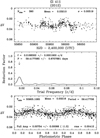 |
Fig. 1 Top panel: Johnson V photometry of Gl 411 from the 2012 observing season, acquired with the TSU T3 0.40 m APT at Fairborn Observatory. Middle panel: frequency spectrum of the 2012 V observations of Gl 411. The best frequency occurs at 0.01683 ± 0.00019 cycles day−1, corresponding to a best period of 59.42 ± 0.67 days. Bottom panel: 2012 V observationsphased with the best period of 59.42 days. The phase curve shows coherent variability with a peak-to-peak amplitude of 0.0075 mag, which we take to be rotational modulation of photospheric spots. Seven of the eight observing seasons exhibit similar modulation (see Table B.1). |
4 Data analysis
4.1 The model
Given an observed velocity time series, {ti, vi, σi}, for i = {1, …, N}, the model for the velocity measurement taken at time ti, vi, can be written, in a very general manner, as:

where mi is the model prediction at time ti and ϵi is the error term. The variation in the radial velocity seen in Fig. 2 is caused by, at least, a combination of instrumental systematics, and a velocity projection effect. These will be the first elements in our model. We will investigate the possibility that either an additional physical acceleration or the effect of an orbiting sub-stellar companion, or both, are also necessary components of the model.
Even after the installation of the octagonal-section fibre in 2011, SOPHIE suffers from a well-observed zero-point change. This effect is monitored by a set of constant stars that are observed regularly, and make up the zero-point velocity “master” (see Courcol et al. 2015; Hobson et al. 2018, for more details). Here, the zero-point master is constructed leaving out Gl 411, which was considered up to now a constant star. Instead of subtracting the measured master from the observations directly, a linear dependence with the zero-point velocity master, vc (ti), was included in the model. In this way, variations which are covariate with the zero-point velocity changes, such as long-term velocity variations, are correctly taken into account. To be able to evaluate vc (ti) at the epochs of the observations of Gl 411, we interpolate the velocities of the constant stars using quadratic splines. In the lower left corner of Fig. 2 the spline interpolation is plotted as a thin red line, and the values at the epochs of the observations of Gl 411 are shown as grey points. In the lower right panel of Fig. 2, a Generalised Lomb Scargle (GLS; Zechmeister & Kürster 2009) of the interpolated zero-point values is presented. The zero-point variations are dominated by a low-frequency variability with period of around 2000 days, followed by peaks at around 450, 300, and and 190 days.
The secular acceleration produced by the changing projection of the star’s velocity vector can be computed using the measured distance, proper motion and absolute radial velocity listed in Table 1 (Kürster et al. 2003). We include this term in the model as well, vp(ti; π, μ, δ), using informative priors on the parallax and proper motion measured at the epoch of the HIPPARCOS catalog, J1991.25, JD = 2 448 349.0625 (Perryman et al. 1997)2, and fixing the star’s declination, δ, to the value in Table 1. For the mean value of the prior distribution, the secular acceleration has an amplitude of about 1.34 m s−1 yr−1. We will call k0d0 the model containing only these two terms, and the expression for the model prediction is then

for model parameters ac, π, μ, and γ0, the systemic velocity at Hipparccos epoch.
We also allow for the possibility of additional variation coming from a secular acceleration, which we model by a linear (d1) or quadratic (d2) term, which produces the model:

where tref is a reference time, taken as JD = 2 457 180, close to the mean time of the SOPHIE time series. The resulting model is called k0d1 if γ2 = 0, and k0d2 otherwise.
Finally, we include the effect of orbiting companions. We assume the effect of multiple companions is simply the sum of the effects of the individual companions (i.e. we neglect mutual interactions between planets). We denote the effect of the individual companions at time ti as vk(ti;θ), where θ is the model parameter vector. vk(ti;θ) is assumed to be a Keplerian function parametrised by the orbital period, P, the amplitude of the radial velocity signal, K, the orbital eccentricity, e, the argument of pericentre, ω, and the mean longitude at a given epoch, L0. Under this parametrisation (see, e.g. Murray & Dermott 2000):
![\begin{equation*} v_k(t_i; \mathbf{\theta}) \,{=}\, K \left[\textrm{cos}\,\left(f_i + \omega\right) + e \textrm{cos}\,(\omega)\right], \end{equation*}](/articles/aa/full_html/2019/05/aa35019-19/aa35019-19-eq6.png)
where fi = f(ti;P, e, ω, L0) is the true anomaly at time ti.
We canthen produce an additional family of models, whose predictions at time ti are:
where n is the number of orbiting companions assumed, and m is the degree of the polynomial assumed for the additional long-term velocity term.
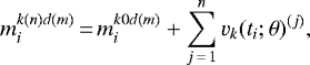
For the error terms ϵi we explored two possibilities. In the first, the error terms are distributed according to a zero-centred multivariate normal with a covariance matrix whose elements are 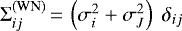 , where σi is the internal uncertainty of the measurement at time ti, σJ is a nuisance parameter called jitter, and δij is the Kronecker delta. In other words, we assume the errors are independent. We call this the white noise (WN) model. Of course, this is strictly not true. Unaccounted-for effects, such as the rotational modulation of the star will translate to correlated errors in our model. Therefore, we also explored the possibility that the error terms are distributed according to a zero-centred multivariate normal with covariance function with elements given by:
where kSE(ti, tj) is the squared exponential kernel function,
with A and τ the covariance amplitude and characteristic timescale, respectively. We call this hypothesis the red noise (RN) model. The chosen kernel function is general enough to describe a wide variety of temporal variations.
Under either of the two possibilities, the likelihood is a multivariate normal centred at the model prediction and with covariance Σ, whose natural logarithm is written
![\begin{equation*} \log\mathcal{L}(\boldsymbol{\theta}) \,{=}\, -\frac{1}{2} \left[ N\log(2\pi) + \log|\Sigma| + \left(\bm{v} - \bm{m}\right)^T \Sigma \left(\bm{v} - \bm{m}\right) \right]\end{equation*}](/articles/aa/full_html/2019/05/aa35019-19/aa35019-19-eq11.png) (1)
(1)
where v and m are N-length vectors containing the velocity measurements and model predictions, respectively.
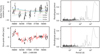 |
Fig. 2 SOPHIE velocities and zero-point offset (upper left and lower left panels, respectively) with their corresponding GLS periodograms (right panels). Upper left panel: the solid and dashed curves represent the additional acceleration and secular (projection) acceleration terms under the three models with largest Bayesian evidence. Lower left panel: the thin red line is the spline interpolation of the zero-point shifts measured on a number of standard stars (see text for details), while the points represent the interpolation evaluated at the epochs of the velocity measurements. Right panels: in the periodograms of SOPHIE raw radial velocities of Gl 411 and zero-point offset of the spectrograph, the vertical red lines mark the frequency of the detected periodic signal. |
4.2 Posterior distribution sampling
The posterior distributions of the model parameters were sampled using the emcee algorithm (Goodman & Weare 2010; Foreman-Mackey et al. 2013), with 300 walkers. The prior distributions are listed in Table A.1. For the parameters  and
and  we added an additional condition so that the eccentricity cannot acquire values above one. The algorithm was run for 25 000 iterations for each model, and we discarded the first 5000 iterations for all models. The chains exhibit adequate mixing and were checked for non-convergence. Summary statistics of the sampled posterior for individual models are presented in Tables C.1–C.4.
The stellar parameters are in excellent agreement between different models, except for the systemic velocity at Hipparccos epoch, γ0, which changes slightly between models with different degree of polynomial acceleration, as expected. The posterior distributions of the stellar proper motion and parallax are dominated by the priors provided by the HIPPARCOS data.
The parameters of the Keplerian curve are also in good agreement across models, but the WN models produce a slightly larger amplitude and shorter period (Fig. 3). The measured maximum-a-posteriori (MAP)-estimates of the RV amplitude range between 1.70 and 1.91 m s−1 – the mean is slightly smaller (see Table 4). The MAP-estimates of the orbital period range from 12.9439 to 12.9477 days.
Concerning the acceleration terms, models with at least a constant additional acceleration are favoured by the data, as shown in Sect. 4.4. The amplitude of the constant acceleration, γ1, depends only slightly on whether a higher degree polynomial is used to describe the data. The MAP-estimates for γ1 under RN models range between −0.49 and −0.37 m s−1 yr−1, which roughly implies companions with periods larger than around 13 yr (twice the observation time span), and with minimum masses above 0.1 Jupiter masses.
The covariance parameters change significantly between models with and without a Keplerian curve. Besides the obvious fact that the additional white noise term is much larger in WN models than in RN models, RN model without a Keplerian curve exhibit a shorter covariance timescale – MAP estimates around 3.8 days for k0 models, and between 8.2 and 9.0 days for k1 models. This is reasonable: the models without a Keplerian curve require the increased flexibility provided by a shorter timescale (Rasmussen & Williams 2005) to explain the full variability present in the time series. In the same sense, models without a Keplerian component also result in slightly larger covariance and white noise amplitudes.
To test the effects of moonlight contamination, we repeated the posterior sampling for the k1d1rn model, but removing either the four observations taken with the Moon closer than 30°, or the 16 measurements acquired with the Moon closer than 35° from Gl 411. In both cases, the results are in excellent agreement with those using the full dataset. We therefore confirm that moonlight contamination is not relevant for this bright target.
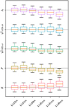 |
Fig. 3 Box plots for Keplerian parameter under all models tested. The boxes extend from the lower to upper quartiles, and the whiskers extend between the 5th and 95th percentiles. The red horizontal lines mark the position of the median. The grey horizontal lines have been chosen conveniently at the median values of the k1d2rn model. |
4.3 Periodogram analysis
Figure 4 presents a series of GLS periodograms of the RV residuals of models of increasing complexity. In every case, the MAP model is subtracted from the RV data presented in Table 2, and the MAP estimate of the additional white noise term, σJ was added in quadrature to the velocity uncertainties. The MAP parameters of each model are listed in Tables C.2 and C.4. In the residuals of the model including only the zero-point correction and a secular acceleration term (k0d0; top periodogram in Fig. 4) powerful peaks are seen at P = 12.945 days and at the frequencies corresponding to the one-day aliases (aliases of one solar day and one sidereal day, 1.0837 and 1.08048 days, respectively). No significance difference is seen between the white and red noise models at this point. Including a linear acceleration term (k0d1) does not reduce the peak powers significantly, as seen in the middle panel of Fig. 4, but slightly changes the frequency at which the maximum occurs to P = 12.959 days.
The peak-to-peak variations of the instrumental zero-point are of the order of 15 m s−1, and mask the presence of the planetary candidate signal (upper right panel of Fig. 2). In the lower right panel of Fig. 2 we show the GLS of the zero-point offset, interpolated at the epoch of observations, which does not show power at the period of the putative signal. It is therefore unlikely that the variability at the P = 12.96 days is introduced by either the zero-point correction or by a coupling of the low-frequency variations and the window function. We nevertheless explore this possibility in much more detail in Sect. 4.5.2.
The largest periodogram power is commonly used as a test statistic to evaluate the significance of the maximum peak in the periodogram. We estimate the corresponding p-values3 by shuffling the residuals 10 000 times (solid horizontal lines in Fig. 4) and computing the maximum peak power in each realisation. The full distribution is estimated by means of a Gaussian kernel density method4, using the resulting powers as input. Under the red noise models, the p-value of the observed maximum peak is estimated to be 9 × 10⁻⁵ under the k0d0 model and 3 × 10⁻⁴, under the k0d1 model. These values are low enough to warrant further investigation.
The third periodogram in Fig. 4 represents the GLS of the residuals of a model including a Keplerian curve (k1d0), with a period around 12.94 days (see Table C.4 for its MAP estimate). Neither of the peaks are present in this figure, and no other peak is seen with power above the 1% p-value level. Some residual power is seen around 55 days, probably related to stellar activity and in agreement with the adopted rotational period, Prot = 56.15 ± 0.27 days, but also possibly due to another planetary companion. However, this peak disappears when a model with a Keplerian curve and a linear acceleration term is considered (k1d1; bottom panel). A long-term periodicity (~ 2000 days) is seen in the bottom panel, but with peak power below the 1% p-value level.
Although the peak at around P = 12.95 days is the strongest one, its 1-day aliases have similar power. The procedure described by Dawson & Fabrycky (2010) was employed in an attempt to identify the real periodicity. The method consists in simulating datasets using the time stamps of the real data, and injecting a sinusoidal signal at each of the candidate periodicities. The amplitudes and phases of the peaks in the periodogram of the resulting synthetic data are compared to the actual observations. The results are shown in Fig. 5, where each row corresponds to a different tested periodicity, indicated by a vertical grey line. The two relevant regions of the periodograms are presented. The blue periodograms are computed for the actual data, and are identical in all three rows. The orange one is computed on each simulated data set. On top of each relevant peak, we present a dial representing the phase of the signal. It seems clear that the peak at 1.0837 days is not a real one; on the other hand, some doubt still remains between thepeak at 12.9478 days and the one at 1.0805 days. The former case reproduces the amplitude of the aliases structure and its phases correctly, in particular the peaks around 1.0835 days and 12.5 days, which are not correctly reproduced with the simulated sinusoid at 1.0805 days. On the other hand, the simulation with a sinusoid at 12.9478 days does not reproduce the peak observed at 1.077 days. The phases do not seem to provide much additional information in this case. In light of this, we assume the real period of the signal to be around P = 12.9478 days, but warn that the other option cannot be fully discarded at this time. In Sect. 6 we present further evidence for the 12.95-day period. In any case, additional high-cadence observations should permit distinguishing between both periods more precisely.
 |
Fig. 4 Radial velocity residuals of the MAP-estimate k0d0rn model (top panel), and generalised Lomb Scargle periodograms under the red noise models. The horizontal lines in the periodogram panels correspond to p-value levels of 0.5, 0.1, 0.01, and 1 × 10⁻³, from bottom to top, and are computed for each dataset by bootstrapping (see text for details). Second from top panel: GLS of radial velocities after zero-point correction and removal of secular acceleration term, that is the residuals of the k0d0model shown in the top panel; third from top panel: residuals of k0d1 model, containing an additional constant acceleration; second from bottom panel: residuals of the k1d0 model, with a Keplerian curve of period P = 12.9438 days; bottom panel: as above, but including also a linear acceleration term in the model (model k1d1). A version of the periodograms using a linear frequency scale in the x-axis is provided in Appendix A (Fig. A.1). |
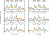 |
Fig. 5 Aliases evaluation. Peak amplitudes and phases in two regions of period space related by daily aliases (left and right columns). Each row contains simulations assuming a given sinusoid period (marked as a grey vertical line in each row) is present in the data. The dials on top of selected peaks indicate the phase at that period. The orange curves and dials correspond to the simulations, while the blue curves and dials are the periodograms computed on the real data, and are identical in all three rows. The simulated data containing a sinusoid at 1.084-day period does not reproduce the amplitudes of the peaks at 1.0805 and 12.95 day. This period is therefore discarded. |
Ancillary observables
Here we study the variability of selected ancillary observables, the bisector velocity span, the FWHM of the CCF, and the activity proxies based on the Hα and Ca II H& K line fluxes. The FWHM and bisector span exhibit a long-term variation that is seen in other stars of the SP3 sample as well. Therefore, we corrected these observables from this effect by subtracting a quadratic fit from the time series.
In Fig. 6 we present the time series and GLS periodograms of these ancillary observables. None of the periodograms exhibit power at the frequency detected in the radial velocity time series. No variation is seen either at the expected rotational period reported in Table 1, around 56 days, nor at the periods of the other estimated rotational periods discussed above. On the other hand, the activity indices based on the Ca II ( ) and Hα lines exhibit some power at periods around 31 days, but with large p-values. Peaks close to one year are also seen in the FWHM time series as well as in the activity proxies, indicating some sort of systematic error still present in SOPHIE data, or an incomplete treatment of the telluric line contamination. In the case of the FWHM, this variability could also be a residual of the window function, due to an incorrect correction for the long-term variation described above. When the 1-year period is subtracted from the data, no other significant periodicities are detected.
Finally, a long-term activity variation is seen, specially in the Hα index, with a maximum in the second to last season. However, other stars observed intensively by the SP3 exhibit a similar increase in the Hα level at this time. In the bottom panel of Fig 6 we also present the time series for Gl 686 (red squares) and Gl 514 (blue triangles), two standard stars used in the SP3, offset to the mean value of the Gl 411 time series. The increase in the Hα level between JD = 2 457 000 and JD = 2 458 000 is seen in all three stars and point to a not-yet-understood systematic effect. We tried to perform a similar analysis for the  time series, but the noise in the
  time-series of these stars is too large to allow us to draw meaningful conclusions. We therefore do not claim detecting a long-term activity variation.
The ancillary observations therefore give no reason to confer an activity or systematic origin to the radial velocity peak at P ~ 12.9 days.
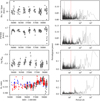 |
Fig. 6 Time series (left panels) and GLS periodograms (right panels) of selected ancillary observables. The best-fit second order polynomials were subtracted from the Bisector Velocity Span and the FWHM time series. The red vertical lines in the periodograms indicate the frequency of the detected planet candidate. In the Hα time series, we also present the data corresponding to two other SP3 targets (see text for details): blue triangles for Gl 514and red squares for Gl 686. A version of the periodograms using a linear frequency scale in the x-axis is provided in Appendix A (Fig. A.2). |
4.4 Model comparison
The periodogram analysis of Sect. 4.3 suggests a periodic component is present in the data with a period of 12.945 days. However, the presence of strong power at this frequency does not provide definitive evidence for the 1-Keplerian model5. Instead, the Bayesian approach allows us to compute the posterior probability of different models and to compare them directly. In particular, the posterior odds ratio between two competing models reduces to the ratio of their marginal likelihoods if equal prior probabilities are assumed.
We used the posterior samples from different models to estimate the corresponding marginal likelihoods via the importance sampling estimator introduced by Perrakis et al. (2014), as implemented by Díaz et al. (2016). This estimate was shown to provide results in agreement with a number of other estimators of the marginal likelihood (Nelson et al. 2018). We further compared the results from preliminary computations with the models employed in this paper using the nested sampling algorithm polychord (Handley et al. 2015). The uncertainty in this determination was estimated through a Monte Carlo approach repeating the computation 100 times. More details on our implementation of the algorithm are given in Appendix A.6 of Nelson et al. (2018).
Although the estimator is known to be biased (Perrakis et al. 2014), it was shown previously that the bias is negligible for sample sizes larger than a few thousands (e.g. Bonfils et al. 2018; Hobson et al. 2018). We verified this by computing the estimator of the marginal likelihood for an increasing number of samples from the joint posterior (Fig. 7). We reach the same conclusion as in previous works. For sample sizes above 1000 or 2000 the bias does not seem significant. The results based on a sample of size 8192 are reported in Table 3.
Overall, it is seen that models containing a Keplerian curve are favoured over models without a Keplerian component. The evidence for models with one Keplerian is much stronger under the red noise models, with Bayes factors above 900. Under the white noise hypothesis, Bayes factors for the k1d1 and k1d0 models are around 48 and 4, respectively, when compared with model k0d1. These are still considered as “strong” and “positive” evidence, respectively, against models without Keplerians (Kass & Raftery 1995). In any case, models accounting for correlation in the data (red noise models) are largely favoured over white noise models, with Bayes factors exceeding 105 for models with one Keplerian. Finally, this computation shows that the data are not sufficient to distinguish between models k1d0, k1d1, and k1d2, but provide a slight preference for the model with a constant acceleration (k1d1). The posterior marginal distributions are similar under all three models with a Keplerian component (Fig. 3).
In view of these results, we decided to produce a sample of the parameter posterior distribution averaged over models, as we did in Bonfils et al. (2018). For this, we resampled the posterior samples obtained for each individual model using the Bayes factors as weights. In Table 4 we provide summary statistics of the marginal distributions of the model parameters and a few additional quantities of interest. In this manner, the Keplerian parameters reported are independent of whether the additional acceleration exists or not, or on the chosen noise model, although in practice, given the strong support for the red noise model, no samples from the white noise models are present in the final merged posterior sample.
In Fig. 2 we present the slowly-varying components of all three models, that is the components remaining after removing the Keplerian contribution. Figure 8 represents the SOPHIE radial velocities, corrected from the MAP-estimate of slowly-varying terms in the model and phase-folded to the MAP period estimate, together with the Keplerian curve (MAP and mean) and its confidence intervals under the most probable hypothesis (k1d1, with correlated noise). The dispersion of the residuals of the MAP model is 2.18 m s−1, which according to our model is produced in almost equal parts by the photon noise plus calibration error, whose mean value is 1.4 m s−1, and the covariance amplitude, whose MAP value is 1.85 m s−1.
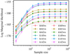 |
Fig. 7 Estimation of the marginal likelihood as a function of the sample size used to compute it. Dashed lines correspond to white noise models, continuous lines to red noise models. The estimator is defined in Perrakis et al. (2014), and the details of the implemention are given in Díaz et al. (2016), Bonfils et al. (2018) and in the Appendix of Nelson et al. (2018). |
4.5 Validation of planetary model
The detected radial velocity signal has the smallest-amplitude detected by the SOPHIE spectrograph so far. We are therefore inclined to be particularly cautious about its origin. In this section, we present a series of tests to validate its planetary origin.
4.5.1 Stacked periodograms
In Sect. 4.3 we showed that none of the activity proxies present clear variability at periods related to the planet candidate signal. Another useful diagnostic for activity is the stacked periodograms, which consists in studying the evolution of the power ofa periodogram peak as the number of observations in the time series is increased (for details, see Mortier & Collier Cameron 2017). A planetary signal should increase its power monotonically, within the limits of the noise, with the number of observations, given that a proper normalisation for the noise level under different sample sizes is taken into account.
In Fig. 9 we present the evolution as the number of data points considered increases of the peak power computed on the residuals of model k0d1, with correlated noise, and normalised according to Eq. (22) in Zechmeister & Kürster (2009). The maximum peak between 12.9 and 13.0 days was considered, to allow for the possibility that the peak position may vary as new data are included. The data points were added chronologically (grey curve and points) or randomly. For the latter case, we produced 10 000 realisations for each number of data points6, changing randomly the order in which the data points were included in the analysed set. The shaded light blue area encompasses the area between the 5th- and 95th-pecentile of the obtained distribution, and the black curve is the mean of the distribution. The normalised peak power increases with the number of points considered, lending support to the hypothesis that the variation is produced byan authentic periodic signal. Additionally, adding the measurements chronologically produces a curve with similar features as the ones obtained by randomly shuffling the data order (thin grey curves), supporting the idea that the signal is not produced by an effect – systematic or activity – occurring at a given moment in the time series.
Log Marginal likelihood ( ) for different models, and Bayes factor with respect to model k1d1 for SOPHIE data.
4.5.2 Possible sampling artefact
Periodicities introduced by the observational sampling can produce spurious detections in radial velocity data (e.g. Rajpaul et al. 2015). In particular, as our model contains low-frequency terms, one may worry that if they are incorrectly accounted for, the window function (Roberts et al. 1987) will be imprinted in the RV time series, producing spurious signals. In this section, we explore if this effect can produce a signal at the frequency of the putative companion.
As a first step, we studied the window function in detail. Besides the strong peaks at and around 1-day and 1-sidereal day, the largest power at periods shorter than 200 days is at a group of peaks around 29.55 days, the Moon synodic period7 (see Fig. 10). The region around the frequency corresponding to the planetary candidate is devoid of strong power. It is therefore unlikely that the low-frequency terms induce a signal at the candidate period.
White noise simulations
To verify this, we generated synthetic data sets sampled at the observing dates of the real SOPHIE observations. The synthetic data contain the effect of the secular acceleration and zero-point correction, but no planet or additional long-term velocity variations were included. The parameters of these effects were randomly drawn from the joint posterior sample of the k1d1rn model, obtained in Sect. 4.2. We added random white noise with a variance equal to the sum of the internal observational error and the inferred jitter (white and correlated), 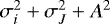 . We generated in this manner 10 000 synthetic radial velocity time series. For each, we fitted the parameters of the k0d0 model using a variation of the Levenberg–Marquardt algorithm implemented in scipy, starting at the MAP-estimate. A GLS was performed on the residuals of the fit, scanning periods between 2 and 200 days, to avoid the obvious peaks coming from the window function. This is similar to what was done to obtain the periodogram in the upper panel of Fig. 4. The maximum power within 0.1 days of the MAP period estimate, 12.947 days, is 0.14. This is to be compared to the value of 0.21 found in the real dataset. Additionally, the number of times the largest peak power appeared in this region was in agreement with what would be expected from white noise. Therefore, a combination of white noise and sampling cannot explain the observed peak at the candidate period. This is actually expected as the long-term variability can be correctly taken into account under these conditions (see discussion in Rajpaul et al. 2015).
Correlated noise simulations
The question remains whether correlated noise could produce a spurious detection. In this case, one may expect the low-frequency variations due to zero-point shifts and the secular acceleration to be masked by correlated noise, leading to an incorrect determination, and hence a residual of the sampling function present in the time series. To explore this, we repeated the experiment described above but including correlated Gaussian noise with a covariance produced by a kernel function of the quasi-periodic type:
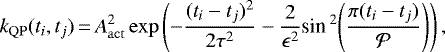
where the four hyper-parameters are the amplitude of the covariance term (Aact), the rotational period of the star ( ), the covariance decay time (τ) and a shape parameter (ϵ). This kernel is known to correctly represent the covariance produced by active regions rotating in and out of view (e.g. Haywood et al. 2014; Rajpaul et al. 2015). To the covariance produced by this kernel, we added a diagonal matrix with the square of the internal data point uncertainties.
For each of the 10 000 synthetic velocity time series produced, the values of the hyper-parameters were drawn from distributions which we claim represent fairly well our knowledge on Gl 411, and the evolution of active regions in general. The parameter representing the rotational period,  , was drawn from a normal distribution with mean 56.15 days, and variance
  , in agreement to our conclusion from Sect. 2. The typical lifetime of the active regions, represented by the parameter τ is
  , where k is randomly drawn from a N(3, 0.22) distribution; the structure parameter ϵ is randomly chosen between 0.5 and 1. For the amplitude Aact, we resorted to the posterior samples of the k0d1 model, for which we computed the quadratic sum of the covariance amplitude – with the squared-exponential kernel – and the additional white noise term:
  . Our ansatz is that Aact is drawn from a normal distribution with mean and standard deviation taken from the covariance diagonal under the k0d1 model, N(2.1 m s−1;0.0484 m2 s-2). In this manner, the simulations will have a similar dispersion around the k0 models as real data does.
None ofthe 10 000 simulations exhibit power in the vicinity of the detected signal as strong as the one observed in the data (Fig. 4). In Fig. 11 the original GLS periodogram8 is presented together with the ten simulated periodograms exhibiting the strongest power within 0.1 days of the MAP-estimate period, 12.948 days. It can be seen that the simulated periodograms are not able to reproduce the observed peak.
Additionally, following Ribas et al. (2018), the distribution of the frequency and power of the largest peaks in the 10 000 simulated periodograms was studied (Fig. 12). As expected, strong power is seen at and around the simulated rotational periods. This is not observed in the real data, suggesting an overestimation of the amplitude of simulated noise. None of the simulated periodograms exhibit the strongest peak at a frequency equal or greater (i.e. farther from the expected rotational signal) than the real peak with as much power. We can therefore provide a conservative upper limit for the p-value for the detected signal under the hypothesis of correlated noise of 1 × 10⁻⁴. Finally, no peak was found – irrespective of whether it constitutes the largest peak in the simulated periodogram or not – at frequencies higher than the detected one and with larger power.
We conclude that correlated noise is extremely unlikely to be the cause of the detected signal, which we therefore attribute to a planetary-mass companion in orbit around Gl 411.
Model parameters averaged over tested models.
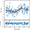 |
Fig. 8 SOPHIE velocities, after subtraction of MAP-estimate model for the zero-point offset, secular acceleration and additional acceleration terms, and phase folded to the MAP-estimate of the Keplerian period, under the k1d1 hypothesis with correlated noise. The black and red curves represent the MAP-estimate and mean Keplerian model over the posterior samples obtained with the MCMC algorithm. The shaded region extends between the 5th- and 95th-percentile model curves, computed over 10 000 randomly chosen posterior samples. |
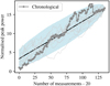 |
Fig. 9 Evolution of the normalised power of the periodogram peak around the planetary candidate period. The GLS periodogram is normalised assuming Gaussian noise remains after removing the signal (Eq. (22) in Zechmeister & Kürster 2009). The grey curve and points correspond to the case where the measurements are added chronologically, while the light blue shaded area encompasses the range between the 5th- and 95th-percentile of the distribution obtained when the data are included in random order. The black curve is the mean of the distribution, and the thin curves are ten draws from the distribution. |
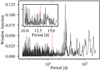 |
Fig. 10 Window function of the SOPHIE observations for periods between 2 and 200 days. The largest peaks in the main panel correspond to the Moon synodic period. In the inset panel we present a zoom around the MAP planet period, indicated in both axes by a vertical dashed line. |
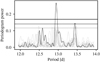 |
Fig. 11 Comparison of the actual GLS periodogram of SOPHIE data (dark curve) and the periodograms obtained from simulated data sets not including a signal at that period. The ten periodograms exhibiting the strongest power at the vicinity of the detected signal among the 10 000 simulated cases are plotted in light grey. The horizontal lines are the 0.5, 0.1 and 0.01 p-value levels, computed as for Fig. 4. |
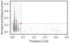 |
Fig. 12 Distribution of the power and frequency of the largest periodogram peaks for 10 000 datasets simulated including only correlated noise. The rotational period and its two first harmonics are indicated by light blue solid and dashed lines, respectively. The red diamond represents the largest peak observed in the real dataset. |
5 Discussion
The analysis from the previous section indicates that the detected signal is produced by a bona fide planetary-mass companion. We discuss here the implications of this result.
5.1 A temperate super-Earth around a nearby star.
Assuming the stellar parameters listed in Table 1, the companion around Gl 411, Gl 411 b, has a minimum mass of 2.99 ± 0.46 M⊕, and the semi-major axis of its orbit is 0.0785 ± 0.0027 AU. This impliesthat the equilibrium temperatures assuming Earth-like and Venus-like Bond albedos (0.3 and 0.8, respectively) are around 350 and 256 K, which are higher than required for the planet to be in the habitable zone (Kopparapu et al. 2013). In Fig. 13 we present a sketch representation of the orbit of Gl 411 b and the location of the habitable zone (Kopparapu et al. 2013). With the current data, a significant eccentricity is not detected. The MAP-estimate eccentricity is around 0.35, but the 95%-HDI for the orbital eccentricity reported in Table 1 includes zero.
Being one of the brightest M-dwarf stars in the sky, Gl 411 is particularly prone for follow-up studies. Searching for transits of Gl 411 b is particularly relevant. Given the relatively small stellar radius, transits of Earth-size planets would produce a decrease of 0.05% in the stellar flux. An educated guess of the planet radius of Gl 411 b can be obtained based on its mass, using the formalism from Chen & Kipping (2017). This gives a radius for the planet of 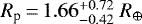 , where the minimum mass was multiplied by 1.15, to account for the unknown orbital inclination angle (Lovis et al. 2017). The posterior transit probability9 is of 2.9%. At the present time, the transit time is known with a precision of over ten hours, and the width of the 95%-HDI for the time of inferior conjunction is around 1.7 days. Therefore, transit search from the ground may be impractical. On the other hand, the Transiting Exoplanet Survey Satellite (TESS; Ricker et al. 2014) and the Characterising Exoplanet Satellite (CHEOPS; Broeg et al. 2013) could search for transits of the planetary companion down to Earth-size objects. However, the former will not observe Gl 411 before late 2019, and the latter is currently scheduled to launch in 2019.
Even in the absence of transits, the proximity of Gl 411 to the Solar system makes its companion an ideal target for atmosphericcharacterisation. In Fig. 14 we place Gl 411 b in the context of the planets detected to date around main sequence stars within 5 pc of the Solar System. It can be seen that Gl 411 b is the second closest planet with a temperate equilibrium temperature, after Proxima Centauri b (Anglada-Escudé et al. 2016), but it is too close to its star to have liquid water on its surface (Kopparapu et al. 2013).
The maximum angular distance between the planet and its star, a(AU)∕d(pc) (Lovis et al. 2017), is around 0.031 arcsec, not unlike Proxima b, which appears at a distance of 0.037 arcsec (Lovis et al. 2017). The planet is therefore not easily resolved by the adaptive optics system on a 10-m class telescope. However, 0.031 arc seconds corresponds to approximately 6 λ∕D at λ = 750 nm, on a 30-m telescope. Additionally, the flux contrast in the visible, estimated as in Lovis et al. (2017) is  , at orbital quadrature, for a geometric albedo of 0.4 and an estimate planetary radius of 1.66 R⊕ (see above). Therefore, the technique of combining high-dispersion spectroscopy and high contrast imaging proposed originally by Sparks & Ford (2002) and demonstrated by, for example, Snellen et al. (2014), Schwarz et al. (2016), and Birkby et al. (2017) should be able to probe the atmosphere of this planet when the next-generation 30-m class telescopes become operational.
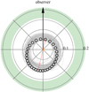 |
Fig. 13 Sketch of the orbit of Gl 411 b, seen from above the orbital plane. The maximum-a-posteriori orbit is indicated with the empty black points that are equally spaced in time over the orbit, and the corresponding major axis is represented by the thin dotted red line. The thin grey lines are a hundred random samples from the merged posterior distributions (see text for details). The host star is at the centre, represented by an orange circle, whose size is to scale. The concentric circles are labelled in astronomical units and the black thick arrow points towards the observer. The filled green area is the inner region of the habitable zone, computed according to Kopparapu et al. (2013). The planet orbits the star too close to be habitable. |
5.2 Previous planet claims
The SOPHIE radial velocities presented here are clearly incompatible with the claims of companions by van de Kamp & Lippincott (1951) and Lippincott (1960), which would produce radial velocity variations of at least 1 km s−1 and of 265 m s−1, respectively. Concerning the companion reported by Gatewood (1996), no information is given on the inclination of the orbit, but assuming the inclination to be i = 45° would produce a radial velocity variation of 18.5 m s−1 over the orbital period of 5.8 yr. No such variation seems possible from the inspection of the RV time series in Fig. 2.
On the other hand, Butler et al. (2017) reported a planet candidate around Gl 411 with a period of 9.8693 days and a mass of 3.8 M⊕, based on long-term monitoring with the HIRES instrument. This signal is absent in the SOPHIE time series, in spite of having sufficient precision to detect it.
We recovered the HIRES radial velocities available from the Vizier catalogue access tool, in order to further explore the missing signal. These are 256 measurements obtained over 17 yr. After removal of a probable outlier velocity acquired on JD = 2 456 494, the measurements have a mean uncertainty of 1.37 m s−1, and a dispersion of3.41 m s−1. We also explored the HIRES data corrected by Tal-Or et al. (2019), who account for a jump due to the instrument upgrade in 2004 and a slow zero-point variation. There are five additional points in this set, at the end of the series, which we disregarded for the analyses. The corrected velocities scatter around the mean with a standard deviation of 3.35 m s−1. The raw periodograms of the HIRES data (Fig. 15) do not show any clear periodicity at the reported period. There existsa forest of peaks between around 5 and 100 days, particularly present in the Vizier version of the data, but no clear predominant variability is observed, not the one reported by Butler et al. (2017) nor the one reported here. With the corrected version of the data, the peak forest is reduced, as well as the peaks at 108 and 185 days. A peak is seen above the noise level at around 34 days.
The absence of the signal at 9.9-day period could be explained by the different model used by the authors, who decorrelated from the activity index based on the Ca II lines, and used a moving average model to reveal the planet. However, no predominant peak is observed in the HIRES residuals of the k0d1 model with correlated noise, described in Sect. 4.1, which should somehow take into account correlated variability as the one produced by activity (the resulting periodograms are very similar to those in Fig. 15).
Nevertheless, we decided to perform an independent analysis in the same line as done for the SOPHIE dataset. Two models with a linear acceleration term and a Keplerian component (k1d1) were explored, one in which the emcee walkers are started in a small region around the period reported by Butler et al. (2017) – although the rest of the parameters were chosen randomly from the prior – and a second one started close to the period detected in the SOPHIE data. We included correlated noise through a squared-exponential kernel and included an additional white-noise term, exactly as done in our analysis above. Irrespective of the data version used, in the first case, the walkers remain around the initial period of about 9.867 days, and the MAP-estimate covariance amplitude and timescale are around 2.65 m s−1, and 2.03 days, respectively, which hint to additional variability in the data not explained by the Keplerian component. Under the model with a Keplerian variability initially set around the period found in SOPHIE data, the walkers expand in period space to occupy all prior space. In other words, no clear preference for the SOPHIE period is found in the HIRES data. It is puzzling that no sign of the signal reported here is seen in the HIRES data. However, no support is provided by the HIRES data for the other period either, independently of the version of the data considered. When the marginal likelihood is computed10 for the model without a Keplerian curve and for the k1d1 model containing a companion at the period reported by Butler et al. (2017), we find that the model without a Keplerian curve exhibits the largest marginal likelihood. If equal prior probability is assumed for the models, this means that, under the current noise model, the model without a Keplerian signal has the largest posterior probability. The marginal likelihoods are reported in Table 5. We decided not to compute the evidence for the model with the period reported in this article, because the corresponding MCMC algorithm, on whose results the computation depends, has clearly not converged.
Of course, under a different noise model, conclusions may change. As mentioned above, the analysis of Butler et al. (2017) differs from ours significantly. A detailed study of the discrepancy found and the missing signal in the SOPHIE data is deferred to a future work. We simply note that the window function of the HIRES data contains a peak exactly at the frequency of the putative planet reported by Butler et al. (2017). Although far from being the most important peak in the window function, the result by Rajpaul et al. (2015) on Alpha Centauri B should cast doubts on the nature of the reported signal, specially when the velocities are known to contain low-frequency terms, such as the secular acceleration, which is here subtracted from the data before performing the analysis.
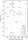 |
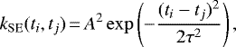
Fig. 14 Equilibrium temperature and distance to the Sun for planets currently known within 5 pc from the Solar System. Equilibrium temperatures were computed assuming circular orbits for all objects, and a Bond albedo of 0.3. Data were obtained from the exoplanets.eu (Schneider et al. 2011) website whenever available. The parameters of the planets are reported in Anglada-Escudé et al. (2014, 2016), Ribas et al. (2018), Hatzes et al. (2000), Benedict et al. (2006), Bonfils et al. (2018), Howard et al. (2014), Feng et al. (2017, 2018), Astudillo-Defru et al. (2017b,c), Burt et al. (2014), Correia et al. (2010), Rivera et al. (2010), Jenkins et al. (2014), Wittenmyer et al. (2014). The limits of thehabitable zone for a star like Gl 411 are indicated by green dotted lines. The symbol sizes are proportional to the natural logarithm of the minimum mass. |
Log Marginal likelihood ( ) for different models, and Bayes factor with respect to model k0d1 for HIRES data.
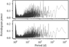 |
Fig. 15 GLS periodograms for HIRES data. Top panel: raw HIRES data obtained from the Vizier catalogue access tool; bottom panel: data corrected by Tal-Or et al. (2019). |
6 Conclusion
Long-term monitoring with the SOPHIE spectrograph revealed a 2.99-Earth-mass planet around the nearby M-dwarf Gl 411 (Lalande 21185, HD 95735) on a 12.95-day period orbit. Gl 411 was one of the standard stars used to follow instrumental velocity systematics before it exhibited a periodic velocity variation. The signal is significantly detected in the SOPHIE data, and ancillary observationsof the line bisector and width, and activity proxies failed to reveal any variability at or around the period of the putative planet. Besides, a series of simulations, assuming both correlated and uncorrelated noise show that the observed signal cannot be produced by a combination of sampling and imperfect consideration of slowly-varying terms in the model. These pieces of evidence point towards the planetary nature of the detected signal.
The alias period at around 1.08 days is also significant, and the current data set is not fully conclusive on which is thereal periodicity. However, the measured occurrence rate of very-short-period planets around low-mass stars is much lower than that of Super-earth planets on 10-day period orbits (Sanchis-Ojeda et al. 2014; Bonfils et al. 2013), which further support our conclusion that the real period of the detected signal is ~ 12.9 days. Nevertheless, additional high-cadence observations would be useful to distinguish between both periods more precisely.
A key component in the validation of the planetary nature of the detected signal is knowledge of the stellar rotational period. Ground-based photometric observations revealed the rotational period of Gl 411 to be around 56 days. Simulations using correlated noise show that the rotational frequency is too different from that of the planetary signal to affect its detection. The planetary signal cannot be reproduced by quasi-periodic variability at the rotational frequency.
Gl 411 b orbits its M2 host star at a distance of approximately 0.079 AU, which implies equilibrium temperatures between 256 and 350 K. The planet orbits inside the inner limit of the habitable zone, and therefore seems too hot to support liquid water on its surface.
The distance to Gl 411 is about 2.55 pc, making the planet Gl 411 b the third closest confirmed exoplanet. The proximity of the system, and its brightness make it an ideal target for future follow-up studies, such as searching for transits of the planet from space. Interestingly, studying the atmosphere of Gl 411 b by combining high-resolution spectroscopy and high-contrast imaging, seems to be in reach of future or even current instrumentation. With the construction of 30-m class telescopes in the northern hemisphere, Gl411 b will become one of the best-suited targets for atmospheric characterisation.
Acknowledgements
We thank all the staff of Haute-Provence Observatory for their support at the 1.93-m telescope and on SOPHIE. We are grateful to J.F. Albacete Colombo for his help with the XMM-Newton observations of Gl 411. This work has been supported by a grant from Labex OSUG@2020 (Investissements d’avenir – ANR10 LABX56). This work is supported by the French National Research Agency in the framework of the Investissements d’Avenir programme (ANR-15-IDEX-02). This work is supported by the French Programme National de Physique Stellaire (PNPS) and the Programme National de Planetologie (PNP). N.A-D. acknowledges the support of FONDECYT project 3180063. X.B. acknowledges funding from the European Research Council under the ERC Grant Agreement n. 337591-ExTrA. G.W.H. acknowledges long-term support from NASA, NSF, Tennessee State University, the State of Tennessee through its Centers of Excellence programme. We acknowledge the support by FCT – Fundação para a Ciência e a Tecnologia through national funds and by FEDER through COMPETE2020 – Programa Operacional Competitividade e Internacionalização by these grants: UID/FIS/04434/2013 & POCI-01-0145-FEDER-007672; PTDC/FIS-AST/28953/2017 & POCI-01-0145-FEDER-028953 and PTDC/FIS-AST/32113/2017 & POCI-01-0145-FEDER-032113. This work has been carried out within the frame of the National Centre for Competence in Research “PlanetS” supported by the Swiss National Science Foundation (SNSF). V.B. and N.H. acknowledge the financial support by the Swiss National Science Foundation (SNSF) in the frame of the National Centre for Competence in Research PlanetS. V.B. has received funding from the European Research Council (ERC) under the European Union’s Horizon 2020 research and innovation programme (project Four Aces; grant agreement No 724427). This research has made use of the SIMBAD database, and of the VizieR catalogue access tool, CDS, Strasbourg, France. The original description of the VizieR service was published in A&AS 143, 23. This work used the python packages scipy (Oliphant 2007; Millman & Aivazis 2011), pandas (McKinney 2010), and matplotlib (Hunter 2007).
Appendix A Additional plots and tables
Parameter prior distributions.
Appendix B Details on the ground-based APT photometry
The 0.40 m automatic photoelectric telescope (APT) at Fairborn Observatory in southern Arizona uses a temperature-stabilized EMI 9924B photomultiplier tube to measure stellar count rates successively through Johnson B and V filters. Gl 411 was measured each clear night in the following sequence, termed a group observation: K,S,C,V,C,V,C,V,C,S,K, in which K is the check star HD 94497 (V = 5.73, B− V = 1.03, G7III:), C is the comparison star HD 95485 (V = 7.45, B− V = 0.40, F0V), V is Gl 411 (V = 7.45, B− V = 0.40, F0V), and S is a sky reading. Three V −C and two K−C differential magnitudes are formed from each sequence and averaged together to create group means. Group mean differential magnitudes with internal standard deviations greater than 0.01 mag were rejected to filter observations taken under non-photometric conditions. The surviving group means were corrected for differential extinction and transformed to the Johnson system. Theexternal precision of these group means, based on standard deviations for pairs of constant stars, is typically ~0.003–0.005 mag on good nights.
Results of the photometric analysis of Gl 411.
Further information on the observations are given in Table B.1, which presents the date range of observations for each season as well as the number of measurements obtained in Cols. 3 and 4, respectively.
Column 5 lists the mean differential magnitudes for each observing season. The V and B seasonal means scatter about their grand means with standard deviations of 0.0021 and 0.0026 mag, respectively. This suggests small brightness variations from year to year may be occurring, but our data set is not long enough to comment on possible brightness (magnetic) cycles.
Finally, the seasonal mean differential magnitudes of the check minus comparison star (K−C) and the seasonal standard deviations are given in Cols. 8 and 9, respectively. The seasonal standard deviations in Col. 9 are consistent with our measurement precision, indicating both the comparison and check stars are constant from night to night. The standard deviations of the V and B seasonal mean magnitudes in Col. 8 scatter about their grand mean with a standard deviation of only 0.0015 mag in both pass bands, indicating the comparison and checks stars are also constant over longer time scales. Further information on the operation of our APTs and processing of the data can be found in Henry (1995a,b, 1999) and Eaton et al. (2003).
Appendix C Posterior summaries for individual models
In this section, we present tables with posterior summaries for all individual models tested. For each model, the maximum-a-posteriori estimate is reported. The number after the ± symbol is the standard deviation for each model. Additionally, the 95%-highest density interval computed on the marginal samples from each parameter is reported in a separate line.
Posterior summaries for individual models without a Keplerian component and assuming white noise.
Posterior summaries for individual models without a Keplerian component and assuming correlated noise.
Posterior summaries for individual models with a Keplerian component and assuming white noise.
Posterior summaries for individual models without a Keplerian component and assuming correlated noise.
References
- Allard, F., Homeier, D., & Freytag, B. 2012, Roy. Soc. London Philos. Trans. Ser. A, 370, 2765 [Google Scholar]
- Allard, F., Homeier, D., Freytag, B., et al. 2013, Mem. Soc. Astron. It. Suppl, 24, 128 [NASA ADS] [Google Scholar]
- Allart, R., Bourrier, V., Lovis, C., et al. 2018, Science, 362, 6421 [Google Scholar]
- Anglada-Escudé, G., Arriagada, P., Tuomi, M., et al. 2014, MNRAS, 443, L89 [NASA ADS] [CrossRef] [Google Scholar]
- Anglada-Escudé, G., Amado, P. J., Barnes, J., et al. 2016, Nature, 536, 437 [NASA ADS] [CrossRef] [PubMed] [Google Scholar]
- Astudillo-Defru, N., Bonfils, X., Delfosse, X., et al. 2015, A&A, 575, A119 [NASA ADS] [CrossRef] [EDP Sciences] [Google Scholar]
- Astudillo-Defru, N., Delfosse, X., Bonfils, X., et al. 2017a, A&A, 600, A13 [NASA ADS] [CrossRef] [EDP Sciences] [Google Scholar]
- Astudillo-Defru, N., Díaz, R. F., Bonfils, X., et al. 2017b, A&A, 605, L11 [Google Scholar]
- Astudillo-Defru, N., Forveille, T., Bonfils, X., et al. 2017c, A&A, 602, A88 [NASA ADS] [CrossRef] [EDP Sciences] [Google Scholar]
- Beichman, C., Benneke, B., Knutson, H., et al. 2014, PASP, 126, 1134 [NASA ADS] [CrossRef] [Google Scholar]
- Benedict, G. F., McArthur, B. E., Gatewood, G., et al. 2006, AJ, 132, 2206 [NASA ADS] [CrossRef] [Google Scholar]
- Birkby, J. L., de Kok, R. J., Brogi, M., Schwarz, H., & Snellen, I. A. G. 2017, AJ, 153, 138 [NASA ADS] [CrossRef] [Google Scholar]
- Boisse, I., Moutou, C., Vidal-Madjar, A., et al. 2009, A&A, 495, 959 [NASA ADS] [CrossRef] [EDP Sciences] [Google Scholar]
- Boisse, I., Eggenberger, A., Santos, N. C., et al. 2010, A&A, 523, A88 [NASA ADS] [CrossRef] [EDP Sciences] [Google Scholar]
- Boisse, I., Bouchy, F., Chazelas, B., et al. 2011, Research, Science and Technology of Brown Dwarfs and Exoplanets: Proceedings of an International Conference held in Shangai on Occasion of a Total Eclipse of the Sun, eds. E. L. Martin, J. Ge, & W. Lin, EPJ Web Conf., 16, 2003 [CrossRef] [Google Scholar]
- Bonfils, X., Delfosse, X., Udry, S., et al. 2013, A&A, 549, A109 [NASA ADS] [CrossRef] [EDP Sciences] [Google Scholar]
- Bonfils, X., Astudillo-Defru, N., Díaz, R., et al. 2018, A&A, 613, A25 [NASA ADS] [CrossRef] [EDP Sciences] [Google Scholar]
- Bouchy, F., Hébrard, G., Udry, S., et al. 2009a, A&A, 505, 853 [NASA ADS] [CrossRef] [EDP Sciences] [Google Scholar]
- Bouchy, F., Isambert, J., Lovis, C., et al. 2009b, EAS Pub. Ser., 37, 247 [CrossRef] [EDP Sciences] [Google Scholar]
- Bouchy, F., Díaz, R. F., Hébrard, G., et al. 2013, A&A, 549, A49 [NASA ADS] [CrossRef] [EDP Sciences] [Google Scholar]
- Broeg, C., Fortier, A., Ehrenreich, D., et al. 2013, EPJ Web Conf., 47, 03005 [CrossRef] [EDP Sciences] [Google Scholar]
- Burt, J., Vogt, S. S., Butler, R. P., et al. 2014, ApJ, 789, 114 [NASA ADS] [CrossRef] [Google Scholar]
- Butler, R. P., Vogt, S. S., Marcy, G. W., et al. 2004, ApJ, 617, 580 [NASA ADS] [CrossRef] [Google Scholar]
- Butler, R. P., Vogt, S. S., Laughlin, G., et al. 2017, AJ, 153, 208 [NASA ADS] [CrossRef] [Google Scholar]
- Chen, J., & Kipping, D. 2017, ApJ, 834, 17 [Google Scholar]
- Correia, A. C. M., Couetdic, J., Laskar, J., et al. 2010, A&A, 511, A21 [NASA ADS] [CrossRef] [EDP Sciences] [Google Scholar]
- Courcol, B., Bouchy, F., Pepe, F., et al. 2015, A&A, 581, A38 [NASA ADS] [CrossRef] [EDP Sciences] [Google Scholar]
- Cutri, R. M., Skrutskie, M. F., van Dyk, S., et al. 2003, 2MASS All Sky Catalog of Point Sources [Google Scholar]
- Dawson, R. I., & Fabrycky, D. C. 2010, ApJ, 722, 937 [NASA ADS] [CrossRef] [Google Scholar]
- Delfosse, X., Forveille, T., Perrier, C., & Mayor, M. 1998, A&A, 331, 581 [NASA ADS] [Google Scholar]
- Delfosse, X., Forveille, T., Ségransan, D., et al. 2000, A&A, 364, 217 [NASA ADS] [Google Scholar]
- Díaz, R. F., Santerne, A., Sahlmann, J., et al. 2012, A&A, 538, A113 [NASA ADS] [CrossRef] [EDP Sciences] [Google Scholar]
- Díaz, R. F., Ségransan, D., Udry, S., et al. 2016, A&A, 585, A134 [NASA ADS] [CrossRef] [EDP Sciences] [Google Scholar]
- Doyon, R., Lafrenière, D., Albert, L., et al. 2014, in Search for Life Beyond the Solar System. Exoplanets, Biosignatures & Instruments, eds. D. Apai & P. Gabor, 3.6 [Google Scholar]
- Dressing, C. D., & Charbonneau, D. 2015, ApJ, 807, 45 [NASA ADS] [CrossRef] [Google Scholar]
- Eaton, J. A., Henry, G. W., & Fekel, F. C. 2003, in Astrophys. Space Sci. Lib., 288, 189 [NASA ADS] [Google Scholar]
- Feng, F., Tuomi, M., Jones, H. R. A., et al. 2017, AJ, 154, 135 [NASA ADS] [CrossRef] [Google Scholar]
- Feng, F., Tuomi, M., & Jones, H. R. A. 2018, MNRAS, submitted [arXiv:1803.08163] [Google Scholar]
- Foreman-Mackey, D., Hogg, D. W., Lang, D., & Goodman, J. 2013, PASP, 125, 306 [CrossRef] [Google Scholar]
- Gaia Collaboration (Brown, A. G. A., et al.) 2018, A&A, 616, A1 [NASA ADS] [CrossRef] [EDP Sciences] [Google Scholar]
- Gaidos, E., Mann, A. W., Lépine, S., et al. 2014, MNRAS, 443, 2561 [NASA ADS] [CrossRef] [Google Scholar]
- Gaidos, E., Mann, A. W., Kraus, A. L., & Ireland, M. 2016, MNRAS, 457, 2877 [NASA ADS] [CrossRef] [Google Scholar]
- Gatewood, G. 1996, American Astronomical Society Meeting Abstracts, 188, 40.11 [Google Scholar]
- Goodman, J., & Weare, J. 2010, Comm. App. Math. Comp. Sci., 5, 65 [Google Scholar]
- Handley, W. J., Hobson, M. P., & Lasenby, A. N. 2015, MNRAS, 453, 4384 [NASA ADS] [CrossRef] [Google Scholar]
- Hatzes, A. P., Cochran, W. D., McArthur, B., et al. 2000, ApJ, 544, L145 [NASA ADS] [CrossRef] [Google Scholar]
- Haywood, R. D., Collier Cameron, A., Queloz, D., et al. 2014, MNRAS, 443, 2517 [NASA ADS] [CrossRef] [Google Scholar]
- Henry, G. W. 1995a, in Robotic Telescopes. Current Capabilities, Present Developments, and Future Prospects for Automated Astronomy, eds. G. W. Henry & J. A. Eaton, ASP Conf. Ser., 79, 44 [NASA ADS] [Google Scholar]
- Henry, G. W. 1995b, in Robotic Telescopes. Current Capabilities, Present Developments, and Future Prospects for Automated Astronomy, eds. G. W. Henry & J. A. Eaton, ASP Conf. Ser., 79, 37 [NASA ADS] [Google Scholar]
- Henry, G. W. 1999, PASP, 111, 845 [NASA ADS] [CrossRef] [Google Scholar]
- Hobson, M. J., Díaz, R. F., Delfosse, X., et al. 2018, A&A, 618, A103 [NASA ADS] [CrossRef] [EDP Sciences] [Google Scholar]
- Houdebine, E. R. 2010, MNRAS, 407, 1657 [NASA ADS] [CrossRef] [Google Scholar]
- Howard, A. W., Marcy, G. W., Fischer, D. A., et al. 2014, ApJ, 794, 51 [Google Scholar]
- Hunter, J. D. 2007, Comput. Sci. Eng., 9, 90 [NASA ADS] [CrossRef] [Google Scholar]
- Jansen, F., Lumb, D., Altieri, B., et al. 2001, A&A, 365, L1 [NASA ADS] [CrossRef] [EDP Sciences] [Google Scholar]
- Jenkins, J. S., Yoma, N. B., Rojo, P., Mahu, R., & Wuth, J. 2014, MNRAS, 441, 2253 [NASA ADS] [CrossRef] [Google Scholar]
- Kass, R. E., & Raftery, A. E. 1995, J. Am. Stat. Assoc., 90, 773 [Google Scholar]
- Kiraga, M., & Stepien, K. 2007, Acta Astron., 57, 149 [NASA ADS] [Google Scholar]
- Kopparapu, R. K., Ramirez, R., Kasting, J. F., et al. 2013, ApJ, 765, 131 [NASA ADS] [CrossRef] [Google Scholar]
- Kürster, M., Endl, M., Rouesnel, F., et al. 2003, A&A, 403, 1077 [NASA ADS] [CrossRef] [EDP Sciences] [Google Scholar]
- Lépine, S., & Gaidos, E. 2011, AJ, 142, 138 [NASA ADS] [CrossRef] [Google Scholar]
- Lippincott, S. L. 1960, AJ, 65, 445 [NASA ADS] [CrossRef] [Google Scholar]
- Lovis, C., Snellen, I., Mouillet, D., et al. 2017, A&A, 599, A16 [NASA ADS] [CrossRef] [EDP Sciences] [Google Scholar]
- Mann, A. W., Feiden, G. A., Gaidos, E., Boyajian, T., & von Braun, K. 2015, ApJ, 804, 64 [NASA ADS] [CrossRef] [Google Scholar]
- McKinney, W. 2010, in Proceedings of the 9th Python in Science Conference, eds. S. van der Walt & J. Millman, 51 [Google Scholar]
- Millman, K. J., & Aivazis, M. 2011, Comput. Sci. Eng., 13, 9 [CrossRef] [Google Scholar]
- Mortier, A., & Collier Cameron, A. 2017, A&A, 601, A110 [NASA ADS] [CrossRef] [EDP Sciences] [Google Scholar]
- Murray, C. D., & Dermott, S. F. 2000, Solar System Dynamics (Cambridge: Cambridge University Press) [CrossRef] [Google Scholar]
- Nelson, B. E., Ford, E. B., Buchner, J., et al. 2018, AAS Journals, submitted [arXiv:1806.04683] [Google Scholar]
- Noyes, R. W., Hartmann, L. W., Baliunas, S. L., Duncan, D. K., & Vaughan, A. H. 1984, ApJ, 279, 763 [NASA ADS] [CrossRef] [Google Scholar]
- Oliphant, T. E. 2007, Comput. Sci. Eng., 9, 10 [CrossRef] [PubMed] [Google Scholar]
- Perrakis, K., Ntzoufras, I., & Tsionas, E. G. 2014, Comput. Stat. Data Anal., 77, 54 [CrossRef] [Google Scholar]
- Perruchot, S., Kohler, D., Bouchy, F., et al. 2008, SPIE Conf. Ser., 7014, 70140J [Google Scholar]
- Perruchot, S., Bouchy, F., Chazelas, B., et al. 2011, in Techniques and Instrumentation for Detection of Exoplanets V, SPIE, 8151, 815115 [Google Scholar]
- Perryman, M. A. C., Lindegren, L., Kovalevsky, J., et al. 1997, A&A, 323, L49 [NASA ADS] [Google Scholar]
- Queloz, D., Henry, G. W., Sivan, J. P., et al. 2001, A&A, 379, 279 [NASA ADS] [CrossRef] [EDP Sciences] [Google Scholar]
- Rajpaul, V., Aigrain, S., Osborne, M. A., Reece, S., & Roberts, S. 2015, MNRAS, 452, 2269 [NASA ADS] [CrossRef] [Google Scholar]
- Rasmussen, C. E., & Williams, C. K. I. 2005, Gaussian Processes for Machine Learning: Adaptive Computation and Machine Learning (Cambridge: The MIT Press) [Google Scholar]
- Ribas, I., Tuomi, M., Reiners, A., et al. 2018, Nature, 563, 365 [NASA ADS] [CrossRef] [Google Scholar]
- Ricker, G. R., Winn, J. N., Vanderspek, R., et al. 2014, in Space Telescopes and Instrumentation 2014: Optical, Infrared, and Millimeter Wave, Proc. SPIE, 9143, 914320 [Google Scholar]
- Rivera, E. J., Laughlin, G., Butler, R. P., et al. 2010, ApJ, 719, 890 [Google Scholar]
- Roberts, D. H., Lehar, J., & Dreher, J. W. 1987, AJ, 93, 968 [NASA ADS] [CrossRef] [Google Scholar]
- Robertson, P., Mahadevan, S., Endl, M., & Roy, A. 2014, Science, 345, 440 [NASA ADS] [CrossRef] [Google Scholar]
- Rosen, S. R., Webb, N. A., Watson, M. G., et al. 2016, A&A, 590, A1 [NASA ADS] [CrossRef] [EDP Sciences] [Google Scholar]
- Sanchis-Ojeda, R., Rappaport, S., Winn, J. N., et al. 2014, ApJ, 787, 47 [NASA ADS] [CrossRef] [Google Scholar]
- Schneider, J., Dedieu, C., Le Sidaner, P., Savalle, R., & Zolotukhin, I. 2011, A&A, 532, A79 [NASA ADS] [CrossRef] [EDP Sciences] [Google Scholar]
- Schwarz, H., Ginski, C., de Kok, R. J., et al. 2016, A&A, 593, A74 [NASA ADS] [CrossRef] [EDP Sciences] [Google Scholar]
- Sellke, T., Bayarri, M., & Berger, J. O. 2001, Am. Stat., 55, 62 [CrossRef] [Google Scholar]
- Snellen, I. A. G., Albrecht, S., de Mooij, E. J. W., & Le Poole R. S. 2008, A&A, 487, 357 [NASA ADS] [CrossRef] [EDP Sciences] [Google Scholar]
- Snellen, I. A. G., Brandl, B. R., de Kok, R. J., et al. 2014, Nature, 509, 63 [NASA ADS] [CrossRef] [Google Scholar]
- Snellen, I., de Kok, R., Birkby, J. L., et al. 2015, A&A, 576, A59 [NASA ADS] [CrossRef] [EDP Sciences] [Google Scholar]
- Sparks, W. B., & Ford, H. C. 2002, ApJ, 578, 543 [NASA ADS] [CrossRef] [Google Scholar]
- Tal-Or, L., Trifonov, T., Zucker, S., Mazeh, T., & Zechmeister, M. 2019, MNRAS, 484, L8 [NASA ADS] [CrossRef] [Google Scholar]
- van Altena, W. F., Lee, J. T., & Hoffleit, E. D. 1995, The General Catalogue of Trigonometric [Stellar] Parallaxes (New Haven, CT: Yale University Observatory) [Google Scholar]
- van de Kamp, P., & Lippincott, S. L. 1951, AJ, 56, 49 [NASA ADS] [CrossRef] [Google Scholar]
- van Leeuwen F. 2007, Hipparcos, the New Reduction of the Raw Data: Astrophysics and Space Science Library (Berlin: Springer Science+Business Media), 350 [Google Scholar]
- Vaughan, A. H., Preston, G. W., & Wilson, O. C. 1978, PASP, 90, 267 [NASA ADS] [CrossRef] [Google Scholar]
- Wittenmyer, R. A., Tuomi, M., Butler, R. P., et al. 2014, ApJ, 791, 114 [NASA ADS] [CrossRef] [Google Scholar]
- Wyttenbach, A., Lovis, C., Ehrenreich, D., et al. 2017, A&A, 602, A36 [NASA ADS] [CrossRef] [EDP Sciences] [Google Scholar]
- Zechmeister, M., & Kürster, M. 2009, A&A, 496, 577 [NASA ADS] [CrossRef] [EDP Sciences] [Google Scholar]
Gl 411 is not included in the latest Gaia data release, probably because of its brightness and/or its high proper motion, which are both cited as sources of incompleteness (see Gaia Collaboration 2018, Sect. 6.2).
For a discussion of common misinterpretations of the p-values and associated issues, see, for example, Sellke et al. (2001).
Because of their relative faintness, SP3 targets are usually avoided around the full moon. Gl 411 is too bright and has a velocity too far from the Moon to be affected, but as this target was considered as a standard star for the SP3, it was not observed when observations of the programme were not performed.
To make a fair comparison, the additional noise term is not added to the uncertainties in this plot. This is the reason why the plot is not identical to the one presented in Fig. 4.
Exactly the same procedure employed in the analysis of the SOPHIE data and described in Sect. 4 was followed here.
All Tables
Log Marginal likelihood () for different models, and Bayes factor with respect to model k1d1 for SOPHIE data.
Log Marginal likelihood () for different models, and Bayes factor with respect to model k0d1 for HIRES data.
Posterior summaries for individual models without a Keplerian component and assuming white noise.
Posterior summaries for individual models without a Keplerian component and assuming correlated noise.
Posterior summaries for individual models with a Keplerian component and assuming white noise.
Posterior summaries for individual models without a Keplerian component and assuming correlated noise.
All Figures
|
Fig. 1 Top panel: Johnson V photometry of Gl 411 from the 2012 observing season, acquired with the TSU T3 0.40 m APT at Fairborn Observatory. Middle panel: frequency spectrum of the 2012 V observations of Gl 411. The best frequency occurs at 0.01683 ± 0.00019 cycles day−1, corresponding to a best period of 59.42 ± 0.67 days. Bottom panel: 2012 V observationsphased with the best period of 59.42 days. The phase curve shows coherent variability with a peak-to-peak amplitude of 0.0075 mag, which we take to be rotational modulation of photospheric spots. Seven of the eight observing seasons exhibit similar modulation (see Table B.1). |
| In the text | |
|
Fig. 2 SOPHIE velocities and zero-point offset (upper left and lower left panels, respectively) with their corresponding GLS periodograms (right panels). Upper left panel: the solid and dashed curves represent the additional acceleration and secular (projection) acceleration terms under the three models with largest Bayesian evidence. Lower left panel: the thin red line is the spline interpolation of the zero-point shifts measured on a number of standard stars (see text for details), while the points represent the interpolation evaluated at the epochs of the velocity measurements. Right panels: in the periodograms of SOPHIE raw radial velocities of Gl 411 and zero-point offset of the spectrograph, the vertical red lines mark the frequency of the detected periodic signal. |
| In the text | |
|
Fig. 3 Box plots for Keplerian parameter under all models tested. The boxes extend from the lower to upper quartiles, and the whiskers extend between the 5th and 95th percentiles. The red horizontal lines mark the position of the median. The grey horizontal lines have been chosen conveniently at the median values of the k1d2rn model. |
| In the text | |
|
Fig. 4 Radial velocity residuals of the MAP-estimate k0d0rn model (top panel), and generalised Lomb Scargle periodograms under the red noise models. The horizontal lines in the periodogram panels correspond to p-value levels of 0.5, 0.1, 0.01, and 1 × 10⁻³, from bottom to top, and are computed for each dataset by bootstrapping (see text for details). Second from top panel: GLS of radial velocities after zero-point correction and removal of secular acceleration term, that is the residuals of the k0d0model shown in the top panel; third from top panel: residuals of k0d1 model, containing an additional constant acceleration; second from bottom panel: residuals of the k1d0 model, with a Keplerian curve of period P = 12.9438 days; bottom panel: as above, but including also a linear acceleration term in the model (model k1d1). A version of the periodograms using a linear frequency scale in the x-axis is provided in Appendix A (Fig. A.1). |
| In the text | |
|
Fig. 5 Aliases evaluation. Peak amplitudes and phases in two regions of period space related by daily aliases (left and right columns). Each row contains simulations assuming a given sinusoid period (marked as a grey vertical line in each row) is present in the data. The dials on top of selected peaks indicate the phase at that period. The orange curves and dials correspond to the simulations, while the blue curves and dials are the periodograms computed on the real data, and are identical in all three rows. The simulated data containing a sinusoid at 1.084-day period does not reproduce the amplitudes of the peaks at 1.0805 and 12.95 day. This period is therefore discarded. |
| In the text | |
|
Fig. 6 Time series (left panels) and GLS periodograms (right panels) of selected ancillary observables. The best-fit second order polynomials were subtracted from the Bisector Velocity Span and the FWHM time series. The red vertical lines in the periodograms indicate the frequency of the detected planet candidate. In the Hα time series, we also present the data corresponding to two other SP3 targets (see text for details): blue triangles for Gl 514and red squares for Gl 686. A version of the periodograms using a linear frequency scale in the x-axis is provided in Appendix A (Fig. A.2). |
| In the text | |
|
Fig. 7 Estimation of the marginal likelihood as a function of the sample size used to compute it. Dashed lines correspond to white noise models, continuous lines to red noise models. The estimator is defined in Perrakis et al. (2014), and the details of the implemention are given in Díaz et al. (2016), Bonfils et al. (2018) and in the Appendix of Nelson et al. (2018). |
| In the text | |
|
Fig. 8 SOPHIE velocities, after subtraction of MAP-estimate model for the zero-point offset, secular acceleration and additional acceleration terms, and phase folded to the MAP-estimate of the Keplerian period, under the k1d1 hypothesis with correlated noise. The black and red curves represent the MAP-estimate and mean Keplerian model over the posterior samples obtained with the MCMC algorithm. The shaded region extends between the 5th- and 95th-percentile model curves, computed over 10 000 randomly chosen posterior samples. |
| In the text | |
|
Fig. 9 Evolution of the normalised power of the periodogram peak around the planetary candidate period. The GLS periodogram is normalised assuming Gaussian noise remains after removing the signal (Eq. (22) in Zechmeister & Kürster 2009). The grey curve and points correspond to the case where the measurements are added chronologically, while the light blue shaded area encompasses the range between the 5th- and 95th-percentile of the distribution obtained when the data are included in random order. The black curve is the mean of the distribution, and the thin curves are ten draws from the distribution. |
| In the text | |
|
Fig. 10 Window function of the SOPHIE observations for periods between 2 and 200 days. The largest peaks in the main panel correspond to the Moon synodic period. In the inset panel we present a zoom around the MAP planet period, indicated in both axes by a vertical dashed line. |
| In the text | |
|
Fig. 11 Comparison of the actual GLS periodogram of SOPHIE data (dark curve) and the periodograms obtained from simulated data sets not including a signal at that period. The ten periodograms exhibiting the strongest power at the vicinity of the detected signal among the 10 000 simulated cases are plotted in light grey. The horizontal lines are the 0.5, 0.1 and 0.01 p-value levels, computed as for Fig. 4. |
| In the text | |
|
Fig. 12 Distribution of the power and frequency of the largest periodogram peaks for 10 000 datasets simulated including only correlated noise. The rotational period and its two first harmonics are indicated by light blue solid and dashed lines, respectively. The red diamond represents the largest peak observed in the real dataset. |
| In the text | |
|
Fig. 13 Sketch of the orbit of Gl 411 b, seen from above the orbital plane. The maximum-a-posteriori orbit is indicated with the empty black points that are equally spaced in time over the orbit, and the corresponding major axis is represented by the thin dotted red line. The thin grey lines are a hundred random samples from the merged posterior distributions (see text for details). The host star is at the centre, represented by an orange circle, whose size is to scale. The concentric circles are labelled in astronomical units and the black thick arrow points towards the observer. The filled green area is the inner region of the habitable zone, computed according to Kopparapu et al. (2013). The planet orbits the star too close to be habitable. |
| In the text | |
|
Fig. 14 Equilibrium temperature and distance to the Sun for planets currently known within 5 pc from the Solar System. Equilibrium temperatures were computed assuming circular orbits for all objects, and a Bond albedo of 0.3. Data were obtained from the exoplanets.eu (Schneider et al. 2011) website whenever available. The parameters of the planets are reported in Anglada-Escudé et al. (2014, 2016), Ribas et al. (2018), Hatzes et al. (2000), Benedict et al. (2006), Bonfils et al. (2018), Howard et al. (2014), Feng et al. (2017, 2018), Astudillo-Defru et al. (2017b,c), Burt et al. (2014), Correia et al. (2010), Rivera et al. (2010), Jenkins et al. (2014), Wittenmyer et al. (2014). The limits of thehabitable zone for a star like Gl 411 are indicated by green dotted lines. The symbol sizes are proportional to the natural logarithm of the minimum mass. |
| In the text | |
|
Fig. 15 GLS periodograms for HIRES data. Top panel: raw HIRES data obtained from the Vizier catalogue access tool; bottom panel: data corrected by Tal-Or et al. (2019). |
| In the text | |
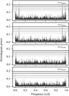 |
Fig. A.1 Same as Fig. 4 but using a linear scale in frequency in the x-axis. |
| In the text | |
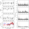 |
Fig. A.2 Same as Fig. 6 but using a linear scale in frequency in the x-axis. |
| In the text | |
Current usage metrics show cumulative count of Article Views (full-text article views including HTML views, PDF and ePub downloads, according to the available data) and Abstracts Views on Vision4Press platform.
Data correspond to usage on the plateform after 2015. The current usage metrics is available 48-96 hours after online publication and is updated daily on week days.
Initial download of the metrics may take a while.