| Issue |
A&A
Volume 622, February 2019
|
|
|---|---|---|
| Article Number | A70 | |
| Number of page(s) | 18 | |
| Section | Stellar structure and evolution | |
| DOI | https://doi.org/10.1051/0004-6361/201833966 | |
| Published online | 29 January 2019 | |
Supernovae from blue supergiant progenitors: What a mess!
1
Unidad Mixta Internacional Franco-Chilena de Astronomía (CNRS UMI 3386), Departamento de Astronomía, Universidad de Chile, Camino El Observatorio 1515, Las Condes, Santiago, Chile
e-mail: This email address is being protected from spambots. You need JavaScript enabled to view it.
2
Department of Physics and Astronomy & Pittsburgh Particle Physics, Astrophysics, and Cosmology Center (PITT PACC), University of Pittsburgh, 3941 O’Hara Street, Pittsburgh, PA 15260, USA
Received:
26
July
2018
Accepted:
11
December
2018
Abstract
Supernova (SN) 1987A was classified as a peculiar Type II SN because of its long rising light curve and the persistent presence of H I lines in optical spectra. It was subsequently realized that its progenitor was a blue supergiant (BSG), rather than a red supergiant (RSG) as for normal, Type II-P, SNe. Since then, the number of Type II-pec SNe has grown, revealing a rich diversity in photometric and spectroscopic properties. In this study, using a single 15 M⊙ low-metallicity progenitor that dies as a BSG, we have generated explosions with a range of energies and 56Ni masses. We then performed the radiative transfer modeling with CMFGEN, from 1 d until 300 d after explosion for all ejecta. Our models yield light curves that rise to optical maximum in about 100 d, with a similar brightening rate, and with a peak absolute V-band magnitude spanning −14 to −16.5 mag. All models follow a similar color evolution, entering the recombination phase within a few days of explosion, and reddening further until the nebular phase. Their spectral evolution is analogous, mostly differing in line width. With this model set, we study the Type II-pec SNe 1987A, 2000cb, 2006V, 2006au, 2009E, and 2009mw. The photometric and spectroscopic diversity of observed SNe II-pec suggests that there is no prototype for this class. All these SNe brighten to maximum faster than our limited set of models, except perhaps SN 2009mw. The spectral evolution of SN 1987A conflicts with other observations in this set and conflicts with model predictions from 20 d until maximum: Hα narrows and weakens while Ba II lines strengthen faster than expected, which we interpret as signatures of clumping. SN 2000cb rises to maximum in only 20 d and shows weak Ba II lines. Its spectral evolution (color, line width and strength) is well matched by an energetic ejecta but the light curve may require strong asymmetry. The persistent blue color, narrow lines, and weak Hα absorption, seen in SN 2006V conflicts with expectations for a BSG explosion powered by 56Ni and may require an alternative power source. In contrast with theoretical expectations, observed spectra reveal a diverse behavior for lines like Ba II 6142 Å, Na I D, and Hα. In addition to diversity arising from different BSG progenitors, we surmise that their ejecta are asymmetric, clumped, and, in some cases, not solely powered by 56Ni decay.
Key words: radiative transfer / hydrodynamics / supernovae: general / supernovae: individual: SN1987A
© ESO 2019
1. Introdution
Although the majority of Type II supernovae (SNe) exhibit a declining bolometric light curve after shock breakout, compatible with the explosion of a red-supergiant (RSG) star, a few per cent of Type II SNe exhibit instead a long rise to optical (and generally bolometric) maximum (Woosley et al. 1988; Kleiser et al. 2011; Pastorello et al. 2012; Taddia et al. 2012, 2016). Owing to this light curve peculiarity, these SNe are classified as Type II-peculiar. While some SNe with a long-rising optical or bolometric light curve can be very luminous at maximum (see, e.g., Terreran et al. 2017), numerous SNe II-pec reach a modest peak V-band brightness, even when characterized by optical spectra with broad (Doppler-broadened) lines.
For SN 1987A, the founding member of the Type II-pec SN class, the Hα line absorption at one day is maximum at about −18000 km s−1 from line center (Phillips et al. 1988; this is amongst the largest values ever recorded for a Type II SN), but the SN peaks about 80 d after explosion with a maximum V-band brightness of only −16 mag (Catchpole et al. 1987; Hamuy et al. 1988; this is fainter than for typical Type II SNe). The basic characteristic that distinguishes SN 1987A and Type II-peculiar SNe from Type II-P SNe is their smaller progenitor radii (Woosley et al. 1988; Woosley 1988; Shigeyama & Nomoto 1990; Utrobin 1993; Blinnikov et al. 2000; Utrobin et al. 2015; Taddia et al. 2016). These works also emphasize that the morphology of SN 1987A and of Type II-pec SN light curves generally requires mixing of 56Ni into the outer progenitor envelope as well as mixing of envelope material (rich in H and He) deep into the progenitor He core. Such mixing is expected theoretically, inferred from nebular phase spectral modeling, and seen in multidimensional hydrodynamical simulations of blue-supergiant (BSG) star explosions (Ebisuzaki et al. 1989; Fryxell et al. 1991; Liu et al. 1992; Li et al. 1993; Kozma & Fransson 1998; Kifonidis et al. 2000, 2003; Wongwathanarat et al. 2013, 2015). While these works present compelling evidence that we can reproduce the observations of SNe II-pec, the modeling has been limited to the photometry, and sometimes only to the bolometric light curve. Radiation hydrodynamical codes employ a variety of techniques for radiation transport, usually treating the gas and the radiation as two separate fluids (see, e.g., discussion in Blinnikov et al. 2000). The gas is however always assumed to be in local thermodynamic equilibrium (LTE) and in steady state.
Spectroscopic modeling of SN 1987A has been done extensively, with successes and problems, using a steady-state non-LTE approach. Hoeflich (1988) finds evidence for departures from LTE as well as evidence for mixing. Eastman & Kirshner (1989) note a problem with the reproduction of He I lines. Schmutz et al. (1990) discuss the difficulty of matching both the absorption and emission parts of Balmer lines, alluding to the presence of clumping. Mitchell et al. (2001) discuss the importance of 56Ni mixing for reproducing Balmer lines at early times, as early as four days after explosion. Mazzali et al. (1992) suggest the need for an overabundance of Ba to reproduce the Ba II lines in the optical at 20–30 days after explosion. Nebular phase spectra also suggest strong macroscopic mixing and a clumpy ejecta (Fransson & Chevalier 1989; Spyromilio et al. 1990; Li et al. 1993; Jerkstrand et al. 2011, 2012).
More recently, simulations have shown that time-dependent effects in the non-LTE rate equations have a critical impact on the strength of Balmer lines and Ba II lines (Utrobin & Chugai 2005). Because of its impact on the ionization, time dependence has been found to impact the formation of all lines and the whole spectrum (Dessart & Hillier 2008). With time dependence, the regions at and above the photosphere are predicted to be more ionized than when steady state is assumed. The assumption of steady state is therefore a shortcoming of older radiative transfer calculations, whose consequences on the conclusions of these works is not known. For example, Schmutz et al. (1990) suggest that clumping may be at the origin of their underestimate of the Hα emission, but this may be attributed to the neglect of time-dependent terms in the non-LTE rate equations. Dessart et al. (2018) find that clumping tends to reduce the Hα line strength, which is the opposite effect proposed by Schmutz et al. (1990). The dominant effect of clumping seen in the simulations of Dessart et al. (2018) is the reduction of the ionization (and therefore the density of free electrons) at and above the photosphere, and the reduction of the Hα emission flux. Mitchell et al. (2001) argue for the need of 56Ni mixing to reproduce Balmer lines at early times but strong Balmer lines can be explained exclusively from a time-dependent effect (Utrobin & Chugai 2005; Dessart & Hillier 2008). These conflicting conclusions about the spectral properties of SN 1987A suggest that the consensus about this SN is at best superficial. It is not clear whether these spectral peculiarities (and our interpretation of their origin) impact the inferences from light curve modeling or alter our understanding of the progenitor and explosion physics. Right now, SN spectral properties are largely ignored (essentially limited to estimating the expansion rate and classifying the SN) when inferring the SN properties. As we emphasize in this paper, the differences in spectral properties for events sharing the same classification as Type II-pec reveal a rich diversity of explosion properties, perhaps even of power sources. So, there is more to Type II-pec SN progenitors than just a reduced radius.
The advantage of performing simulations of the bolometric light curve using radiation hydrodynamics, or of the spectra using steady-state radiative transfer, is the speed at which one can generate results and iterate until a good match is obtained. This advantage is however offset by the lower level of consistency of the approach since the successful model only reproduces a fraction of the constraints. In Dessart & Hillier (2010) and Li et al. (2012), we presented non-LTE time-dependent simulations for one ejecta model and compared to the observations of SN 1987A. With our approach, we could reproduce H I and He I lines at early times, even in the absence of non-thermal processes. At the recombination epoch, the time dependent treatment captured the ionization freeze-out and allowed us to reproduce H I lines. At late times, non-thermal processes (combined with strong inward mixing of H) are essential to retain a strong Hα line. But our studies were limited to one ejecta model. They were also started at 0.3 d when the ejecta was not in homologous expansion. To accommodate the assumption of homology in CMFGEN, we had to force it, which affected the initial structure of our simulations. Overall, these simulations yielded significant departures from the observations of SN 1987A, although qualitatively, its basic photometric and spectroscopic properties were satisfactorily reproduced in our ab-initio approach.
Here we revisit our previous modeling of BSG star explosions. We present simulations based on one BSG progenitor model whose characteristics are close to those proposed for the prototypical Type II-pec SN 1987A (in particular, its progenitor radius of about 50 R⊙; Arnett et al. 1989). However, this model is now used to generate a wide range of ejecta models characterized by different explosion energies, 56Ni mass, H to He abundance ratio, or chemical mixing. We confront our results to SN 1987A as well as other Type II-pec SNe observed since, including 2000cb, 2006V, 2006au, 2009E, and 2009mw (Kleiser et al. 2011; Pastorello et al. 2012; Taddia et al. 2012, 2016; Takáts et al. 2016). This sample of SNe II-pec allows us to step back from SN 1987A and consider the SN II-pec class at large. Our simulations, based on smooth and spherically-symmetric ejecta, allow us to gauge how clumpy and asymmetric each SN ejecta may be, as well as discuss the power source at the origin of the SN luminosity.
In the next section, we present the set of observations used in this study. In Sect. 3, we present our numerical approach, describing how the progenitor model was produced, how the explosion was generated, and how we compute the radiative properties of the resulting ejecta. We then present the results from our simulations, starting with the UVOIR light curves (Sect. 4), followed by the V-band and optical color evolution (Sect. 5), and the spectral properties (Sect. 6). In Sect. 7, we comment on the structure of the photospheric layers, and in particular on the offset between the location of the photosphere and the location of the recombination front in our Type II-pec SN ejecta. We then compare our model results with the observed photometric and spectroscopic properties of Type II-pec SNe (Sect. 8). Finally, we present our conclusions in Sect. 9.
2. Observations
To compare our models to observations, we use photometric and spectroscopic data for a sample of Type II SNe having an optical or bolometric light curve with a long rise to maximum. In practice, we selected SNe 1987A, 2000cb, 2006V, 2006au, 2009E, and 2009mw (this is not meant to be an exhaustive list). Below, we summarize the basic characteristics of each SN (see also Table 1) and the source of the observational data used. The data was downloaded from the SN catalog (Guillochon et al. 2017)1 and from WISEREP (Yaron & Gal-Yam 2012)2.
2.1 SN 1987A
For SN 1987A, we used spectra from Phillips et al. (1988) for the first 130 d and from Phillips et al. (1990) for later times. For the inferred bolometric light curve, we used both the results of Hamuy et al. (1988) and Catchpole et al. (1987; which differ, in part, from the different values of the adopted reddening, i.e., 0.15 and 0.2 mag). For the photometry, we use the data from these papers. We adopted the time of the neutrino burst at MJD 46849.82 as the time of explosion for SN 1987A (Hirata et al. 1987; Bionta et al. 1987). We used a recession velocity of 286.5 km s−1 (redshift of 0.00096), from Meaburn et al. (1995). We adopted a reddening E(B – V) = 0.15 mag and a distance modulus of 18.5 mag (equivalent to a distance of 50 kpc).
2.2 SN 2000cb
Following Kleiser et al. (2011), we adopted a distance of 30.0 Mpc, a reddening E(B – V) of 0.114 mag, and a redshift of 0.0064. We adopt the explosion date MJD 51657.0 (i.e., one day later than the value adopted by Kleiser et al. 2011) since it yields a better match to the early time spectra and optical color of model a5 (Sect. 8.1).
2.3 SN2006V
For SN 2006V, we use the photometric and spectroscopic data from Taddia et al. (2012). We adopted a distance of 72.70 Mpc, a redshift of 0.0158, a reddening E(B – V) = 0.029 mag, and an explosion date of MJD 53748.0 (Taddia et al. 2012). SN 2006V shows a number of peculiarities, and most notably its persistent blue optical color and the anomalously weak Hα absorption during the first two months after explosion, combined with the absence of O I 7774 Å.
2.4 SN 2006au
For SN 2006au, we use the photometric and spectroscopic data from Taddia et al. (2012). We adopted a distance of 46.20 Mpc, a redshift of 0.0098, a reddening E(B – V) = 0.312 mag, and the explosion epoch of MJD 53794.0 from Taddia et al. (2012).
This high reddening implies a spectrum with a blue color at the recombination epoch, just like for SN 2006V, and in contrast with SN1987A (Taddia et al. 2012). Physically, a very low, sub-LMC, metallicity (together with a very weak mixing of core metals into the H-rich layers) might explain such a blue color (see the models of Dessart et al. 2013, and the recent observations of SN 2015bs for which a very low metallicity of 0.1 Z⊙ is inferred; Anderson et al. 2018). SNe 2006V and 2006au are both located far out in the spiral arms of their host galaxy, so a very low metallicity is possible for both. Another possibility is that the reddening toward SN 2006au is in fact negligible. In this case, the intrinsic brightness and the optical colors of SN 2006au would be comparable to those of SN 1987A (see Sect. 8.6 for discussion).
2.5 SN 2009E
Following Pastorello et al. (2012), we adopted a distance to SN 2009E of 29.97 Mpc, a reddening E(B – V) = 0.04 mag, a recession velocity of 2158 km s−1 (redshift of 0.00720), and the explosion date MJD 54832.5. Although it depends on the adopted reddening, the offset in optical brightness with SN 1987A is small.
2.6 SN 2009mw
We use the photometric and spectroscopic data for SN 2009mw of Takáts et al. (2016). The optical light curve of SN 2009mw is similar to that of SNe 1987A and 2009E (Takáts et al. 2016). The spectroscopic data may have some calibration issues. The first spectrum has an unusual slope long-ward of 8000 Å, while the second epoch has a bluer color than either the first or the third spectrum. In the present comparison we have ignored the second spectrum. Following Takáts et al. (2016), we adopted a distance of 50.95 Mpc, a reddening E(B – V) of 0.054 mag, a redshift of 0.0143, and an explosion date of MJD 55174.5. The explosion date is uncertain.
3. Initial conditions and methodology
Our model set is limited to one progenitor star, hence to a single progenitor mass. We use a 15 M⊙ progenitor because this represents a standard mass for a massive star. The progenitor radius of 50 R⊙ is typical for a BSG star, which is thought to be the defining characteristic of SNe II-pec compared to SNe II-P or II-L. We adopt an ejecta metallicity typical of the LMC since it is thought to be representative of SNe II-pec (Taddia et al. 2016). We enforce a strong mixing since this property has been inferred by all light curve calculations of SN 1987A (see, e.g., Blinnikov et al. 2000). These results allow us to narrow the vast parameter space one would ideally like to cover, which includes a range of progenitor radii, masses, metallicities, explosion energies, 56Ni mass, 56Ni mixing. Covering all permutations would be a major task with any code.
3.1 The progenitor model
Our study is based on a non-rotating zero-age main sequence star of 15 M⊙. This initial model is evolved with MESA (Paxton et al. 2011, 2013, 2015) at a metallicity of 10−7. It reaches core collapse after 12.88 Myr (the MESA simulation is stopped when the maximum infall velocity reaches 1000 km s−1). At that time, the surface luminosity is 57400 L⊙, the surface radius is 44.8 R⊙, the effective temperature is 13350 K, the total mass is 14.99 M⊙, the CO core mass is 2.83 M⊙, the He core mass is 4.07 M⊙, and the mass of the H-rich envelope is 10.92 M⊙. Hence, with this very low metallicity the model reaches core collapse as a BSG star rather than a RSG star without any tinkering of convection parameters or the introduction of rotation etc. We show some properties of this model at the onset of core collapse in Fig. 1.
3.2 Explosion models
The explosion is simulated with V1D (Livne 1993; Dessart et al. 2010a,b) by setting up a thermal bomb at the Lagrangian mass cut of 1.55 M⊙. The binding energy of the overlying envelope is 4 × 1050 erg. Energy is deposited at a depth-independent rate in the inner 0.05 M⊙ for 0.5 s. This rate is chosen to produce a set of ejecta with a kinetic energy at infinity of 0.4, 0.8, 1.2, and 2.4 × 1051 erg. In this order, this set corresponds to model names a2, a3, a4, and a5 (model a1 with half the energy of model a2 exhibits strong fallback and is excluded from the study). By varying the explosion energy, we mimic the effect of varying the ejecta (or the progenitor) mass.
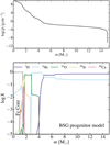 |
Fig. 1. Density (top panel) and composition (bottom panel) profiles of our 15 M⊙ model at the onset of core collapse. The model corresponds to a BSG star with a surface radius of 44.8 R⊙. The adopted environment metallicity is 10−7. The bulk of the composition is H and He rich, and the metal-rich part is limited to the He-core below a lagrangian mass of 4 M⊙ (see Sect. 3.1 for discussion). |
In this study, we want to have a 56Ni mass that increases with explosion energy and is in rough correspondence to observed values (e.g., for SN 1987A; Arnett et al. 1989). In simulations, the 56Ni mass is sensitive to the explosion trigger (energy, power, mass cut location) so it is hard to control. Hence, at 5 s after the explosion trigger in the V1D simulations, we reset the 56Ni mass to be 0.02 (model a2), 0.04 (a3), 0.08 (a4), and 0.16 M⊙ (a5). When rescaling the 56Ni mass fraction, we renormalize all other mass fractions at each depth so that the sum of mass fractions is unity. In model a4ni (a3ni), the 56Ni mass fraction is scaled by a factor of three (two) compared to model a4 (a3). In model a4he, we scale by a factor of 0.658 the hydrogen mass fraction in the MESA model at the time of collapse, while the difference in total mass fraction at each depth is transferred to helium to keep the normalization to unity. This scaled MESA model is then exploded the same way as model a4.
In each model, we imposed a mixing of all species in mass space. At 5 s after the explosion trigger, we stepped through each ejecta mass shell mi and mixed all mass shells within the range [mi, mi + δm]. In all but one model, we adopted δm = 4 M⊙. In model a3m, we used δm = 2 M⊙. Because of the moderate or strong mixing adopted in all models, the low metallicity of the progenitor star is largely erased since a significant amount of intermediate mass elements (IMEs) and iron-group elements (IGEs) are mixed throughout the ejecta all the way to the outer layers. Mixing takes place primarily during the early dynamical phase of the explosion and is largely over when the reverse shock, which travels inward into the former He-core material, dies out. We assume that this mixed composition profile is subsequently frozen in (the only changes are associated with the local decay of unstable isotopes).
Ejecta properties for our model set used as initial conditions for the CMFGEN calculations.
Apart from the initial 56Ni abundance (and the different levels of mixing between models a3 and a3m), all models (except model a4he) have the same composition in mass space (this stratification differs in velocity space if the ejecta kinetic energy is different). In the outer regions of the ejecta, the mass fraction for the main species are 0.695 for H, 0.271 for He, 0.0037 for C, 0.017 for O, 0.0027 for Si, and 0.00058 for Fe (N has a negligible mass fraction). In model a4he, the surface mass fractions for H and He are 0.457 and 0.509. With this set, we can explore the effects of ejecta kinetic energy (a2, a3, a4, a5; models also differ in 56Ni mass), 56Ni mass (for about the same ejecta mass and kinetic energy; a3 and a3ni; a4 and a4ni), 56Ni mixing (a3 and a3m), and H/He abundance ratio (a4 and a4he).
3.3 Radiative transfer models with CMFGEN
At 1 d after the explosion trigger, the ejecta are all close to homologous expansion. The V1D simulations are then remapped into CMFGEN (Hillier & Miller 1998; Dessart & Hillier 2005, 2008; Hillier & Dessart 2012; Dessart et al. 2013). To avoid repetition, we refer the reader to these papers for details about the numerical approach and setup.
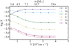 |
Fig. 2. Composition profiles for the inner ejecta of model a2 used in the initial CMFGEN model at 1.1 d (the dashed curve corresponds to 56Ni). The outer ejecta has the same composition as the one at 4000 km s−1. The total ejecta mass for model a2 is 14.30 M⊙. Other models have similar profiles because they all stem from the same progenitor. Differences arise from differences in explosion energy, 56Ni yield, and mixing. Hence, other models show composition profiles that are shifted horizontally (i.e., in velocity space) or vertically (i.e., in yield, which is most relevant for 56Ni, or for H and He in model a4he; see Sect. 3.2 for discussion). |
In V1D, the smoothing applied at 5 s erases the sharp variations in composition. However, strong density variations are present in the models at 1 d (caused by the density contrast between progenitor He core and H-rich envelope, which is exacerbated by the reverse shock that it causes). We apply a gaussian smoothing to damp these strong variations in density. In the regions interior to the inner boundary, we use a linear extrapolation for the density. Because the density steeply rises at the base (the more so in the weaker explosion models), it alters the resulting ejecta mass. Hence, the CMFGEN ejecta properties differ from those obtained with V1D. This primarily concerns the innermost layers at the lowest velocities, and thus affects the ejecta mass (by up to 7%), the scaled 56Ni mass (by up to 25%), and the kinetic energy aimed for (by up to ∼15%, which arises mostly because of the change in ejecta mass). Since the offset in ejecta mass stems mostly from a change in density in the innermost ejecta layers rich in metals, we suspect the impact on the light curve will be modest. The ejecta properties used for our simulations with CMFGEN are presented in Table 2 and the ejecta composition profile for model a2 is shown in Fig. 2.
The low nitrogen content in the progenitor and in our ejecta (about 0.0001 M⊙) is a result of using a very low metallicity progenitor. But nitrogen has no influence on the SN light curves and no nitrogen line is observed in SNe II-pec. Such limitations have little impact on our results. Instead, with strong mixing, the spectrum forms in a metal-rich environment a few weeks after explosion, irrespective of the adopted progenitor metallicity.
Metals like Ba, not included in MESA nor in V1D, are given a constant mass fraction equal to the corresponding LMC metallicity value. Metals between Ne and Ni that are included in MESA and V1D are given a minimum mass fraction equal to the corresponding LMC metallicity value (this applies to the most abundant stable isotope for each element). The LMC value is adopted here since it is the metallicity inferred for the environments of Type II-pec SNe (Taddia et al. 2013).
The numerical setup is comparable to that of Dessart et al. (2013). We use the same model atoms (with the addition of Ba), with updates to the atomic data (in particular for Fe and Co) as described in Dessart et al. (2014). We treat the following ions: H I, He I- II, C I- Ⅲ, N I- II, O I- III, Ne I- II, Na I, Mg I- III, Si I- III, S I- III, Ar I- II, K I, Ca I- III, Sc I- III, Ti II- III, Cr II- IV, Fe I- V, Co II- V, Ni II- V, and Ba I– II.
In our CMFGEN simulations, the intrinsic line width is set by the effective thermal velocity Vth, which is controlled by the local gas temperature T, the atomic mass A of the element or ion, as well as the adopted micro-turbulent velocity of the medium Vturb. We use the definition
 (1)
(1)
where mu is the atomic mass unit and kB is the Boltzmann constant. If the turbulent velocity is zero, the line width at 10 000 K decreases from about 10 km s−1 for H I lines down to about 1 km s−1 for an Fe line. The broader is the intrinsic width of lines, the smaller is the total number of frequency points used in CMFGEN (we use a fixed number of frequency points, typically 5–6, to resolve a given line; line overlap does not increase the number of allocated frequencies). In the present set of simulations, the number of frequency points is ∼100 000 for Vturb = 50 km s−1 and ∼500 000 for Vturb = 10 km s−1. The computational cost of running CMFGEN with a small value of Vturb is non trivial.
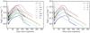 |
Fig. 3. Left panel: UVOIR light curves for our CMFGEN simulations, together with the inferred light curve for SN 1987A (the shaded area is bounded by the UVOIR light curves inferred by Catchpole et al. 1987 and Hamuy et al. 1988). Right panel: same as left, but now for the simulations a2, a3, a4, and a5 (which differ primarily in ejecta kinetic energy and 56Ni mass). We also show the total decay power emitted (dashed line) and absorbed (dash-dotted line) for each model. |
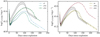 |
Fig. 4. Left panel: same as Fig. 3, but now for the simulations a3, a3m, and a3ni (which differ in chemical mixing magnitude and in 56Ni mass). Right panel: same as left, but now for the simulations a4, a4he, and a4ni (which differ in H/He ratio in the progenitor H-rich envelope and in 56Ni mass). |
Exceptionally, for this study, all simulations were performed with a turbulent velocity of 10 km s−1, except for the low energy model a2. The simulations for this ejecta model were taking an eternity to converge with 10 km s−1 and so were stopped after 37 time steps, at a SN age of 31.14 d – the time sequence for model a2 is thus performed with a turbulent velocity of 50 km s−1. Model a4 was run both with 10 km s−1 and 50 km s−1 (the latter corresponds to model Bsm in Dessart et al. 2018). Hence, for models a2 and a4, we have two sequences (truncated at 31.14 d for a2) performed with a turbulent velocity of 10 km s−1 and 50 km s−1. Comparison of the two reveal that the bolometric light curves are identical to within 1% at all times and the optical colors differ modestly. Simulations performed with the lower value of Vturb have bluer optical colors, typically by ≲ 0.1 mag. This is caused by the enhanced line blanketing induced by a larger value of Vturb. The models with a greater turbulent velocity have a larger Rosseland mean optical depth but this does not impact the light curve. The reason is that there is effectively no diffusion from large optical depth. What matters is diffusion through the photospheric layers, and for that part, the turbulent velocity seems to impact the redistribution of flux (the color) rather than its escape (the total flux). So, the use of a larger value of Vturb has little impact on the current results.
The present simulations include only the radioactive decay of 56Ni and 56Co. All other isotopes are considered stable (most are). We compute the non-local energy deposition at all epochs using a purely absorptive treatment and a gray opacity of 0.06 Ye cm2 g−1 (Ye is the electron fraction). We treat the associated non-thermal processes within the non-LTE time-dependent solver of CMFGEN (for details, see Dessart et al. 2012 and Li et al. 2012).
While preparing this article, Dessart et al. (2018) published a study on the effect of clumping in Type II SNe during the photospheric phase. Using a volume filling factor approach, and ignoring any impact from porosity and chemical segregation, they find that clumping enhances the recombination rate, causing the photosphere to recede faster through the ejecta and boosting the luminosity. This clumping effect leads to a shorter rise time to maximum and an earlier transition to the nebular phase. In other words, all else being the same, a clumped ejecta tends to behave as a smooth ejecta of a lower mass. Clumping is ignored in this study.
With CMFGEN, doing the eight time sequences presented here was a major endeavor. Each time sequence represents 65 time steps, each taking between two days and a week of computing. The total number of models or epochs is 520 and required more than six months of computing. Doing more with our current super-computer resources is not possible.
4. UVOIR light curves
Figures 3 and 4 show the UVOIR light curve for our set of models3. In the left panel of Fig. 3, we show the whole set of models together with the inferred UVOIR light curve of SN 1987A (Catchpole et al. 1987; Hamuy et al. 1988). All models exhibit a similar light curve morphology, with a ∼100 d rise to a ∼50 d broad maximum. In all cases the rise time is longer than observed for SN 1987A, and the width of the maximum is also broader. The brightening rate on the way to maximum is lower than for SN 1987A unless the 56Ni mass is well in excess of the value inferred for SN 1987A (which is about 0.08 M⊙, depending on the adopted reddening and the amount of flux not accounted for).
In the right panel of Fig. 3, we only show the set of models a2, a3, a4, and a5, which differ primarily in ejecta kinetic energy and 56Ni mass. However, we now add the total decay power emitted and absorbed. The difference between the latter two arises from γ-ray escape. The weaker explosions trap more efficiently γ-rays. For the more energetic explosions corresponding to models a4 and a5, γ-ray leakage starts at or soon after maximum. The difference between the total decay power absorbed and the UVOIR luminosities at nebular times arises from the flux not accounted for that falls beyond 2.5 μm (at earlier times the luminosity is affected by optical-depth effects). As time progresses in the nebular phase, the UVOIR luminosity converges toward the total decay power absorbed (or the bolometric luminosity).
We find that the bolometric luminosity at maximum is typically 40–60% larger than the total decay power absorbed at that time. The SN 1987A light curve shows a similar offset.
The slopes at nebular times all follow closely the 56Co decay slope for full trapping. In models a2–a3, this arises because full trapping holds. In models a4–a5, it arises because the increasing γ-ray escape fraction is compensated by the enhanced fraction of the flux falling between 1000 Å and 2.5 μm (that fraction recorded by the UVOIR luminosity).
These variations in brightness are in part reflected by the evolution of the conditions at the photosphere (Fig. 5). The initial drop in luminosity stops at about 5 d when the photospheric temperature stabilizes at the H recombination temperature. Then, as the photospheric radius increases, the luminosity also increases, reaching a maximum when the photospheric radius is also maximum (having values in the range 1–3.5 × 1015 cm).
Figure 4 shows two subsets of models having the same ejecta mass and kinetic energies but differing in composition. Models with enhanced 56Ni are more luminous at all times than their counterpart with less 56Ni. At the earliest times, the offset is small because 56Ni decay power has only a small influence on the outer layers from where the radiation escapes. The offset is however not zero because the mixing is strong in our ejecta models. For example, model a3m is fainter than model a3 because it has less 56Ni and weaker 56Ni mixing (the ejecta mass is also lower by 1 M⊙). Model a3ni is more luminous than models a3 and a3m because it has twice as much 56Ni, which is also strongly mixed. These dependences are well understood and have been discussed extensively in the past (see, e.g, Shigeyama & Nomoto 1990 or Blinnikov et al. 2000). Model a3 and its variants do not match well the UVOIR light curve of SN 1987A, but the spectral evolution of model a3 is a good match to SN 1987A beyond ∼15 d.
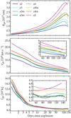 |
Fig. 5. Evolution of the radius, velocity (which can also be deduced directly from the radius and the time elapsed since explosion), and temperature at the photosphere for our set models. The insets in the lower two panels zoom on the epoch around bolometric maximum, when the differences in velocity and temperature between models are harder to discern. |
In the right panel of Fig. 4, we show the UVOIR light curves for model a4 and a4he. The two models have very similar 56Ni mass (and the same ejecta mass) but model a4he has more He and less H – the abundance profile for He and H are qualitatively the same in both models, except that the profile for He (H) is shifted to a greater (lower) mass fraction in model a4he (see for reference the composition shown in Figs. 1 and 2). The composition profile of model a4he is more characteristic of the RSG composition of the models produced in Dessart et al. (2013). The comparison of models a4 and a4he shows that the He content of the envelope matters – see, e.g., Fig. 6 of Kasen & Woosley (2009) for a similar study in the context of Type II-P SNe. The greater the He content (or equivalently the lower the H content), the faster the rise to maximum. The model is brighter earlier and fainter later, essentially at constant total time-integrated bolometric luminosity (the comparison is not exact here since the 56Ni mass differs by 7% between the two models; with the same 56Ni mass, model a4he would have been a little brighter earlier on, and its maximum luminosity would have been greater, increasing the contrast with model a4). The origin of the light curve differences is that the lower the H content, the greater the He content, the harder it is to keep the gas ionized. Consequently, the gas at and above the photosphere recombines more efficiently, allowing the photosphere to recede faster. Compare to model a4, model a4he has a photosphere that is more compact and hotter by 5–10% on the way to bolometric maximum (Fig. 5). This speeds up the recession of the photosphere and the release of stored energy. For the same amount of stored energy (arising from shock-deposited energy and 56Ni decay heating), the greater helium content shifts the light curve left ward, acting as if the ejecta mass is smaller. These effects are similar to those arising from clumping (Dessart et al. 2018). With clumping, model a4he may become close to matching the SN 1987A light curve.
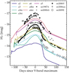 |
Fig. 6. Comparison of the V-band light curves for observed SNe II-pec and for our set of models (the time axis corresponds to the time elapsed since V-band maximum; this time is not accurately known given the width of the light curves and the noise in the observed photometry). If we were to use a negligible reddening for SN 2006au (see Sects. 2.4 and 8.6), its optical brightness and color would be comparable to those of SN 1987A. The V-band light curve of SN 2009mw is very similar to that of SN 2009E and thus not shown (Takáts et al. 2016). The SN properties used to make this figure are listed in Table 1. |
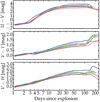 |
Fig. 7. Evolution of the U – V, V – I, and V – H colors for our set of models. |
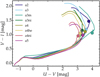 |
Fig. 8. Color-color diagram for our set of models. The filled dot indicates the time of bolometric maximum – all models start in the bottom-left corner with a blue optical color. |
Our CMFGEN light curves are qualitatively similar to those published before for BSG explosions (see, e.g., Woosley et al.1988; Shigeyama & Nomoto 1990; Blinnikov et al. 2000). For example, the model 14E1 (with strong mixing) of Shigeyama & Nomoto 1990; see their Table 2 and Fig. 16) appears similar to our model a4 (or a4he) and yields a similar bolometric light curve, brighter early on, rising slightly faster and peaking at a brighter bolometric maximum. Our models a4 and a4he match the SN 1987A light curve better at early times but less well around the time of maximum (model a4he peaks about 10 d later than SN 1987A). As argued in Dessart et al. (2018), a faster rise and an earlier peak can be obtained by invoking clumping. Blinnikov et al. (2000) obtain similar results to Shigeyama & Nomoto (1990) for the same progenitor. Numerous other studies have been published, pointing to similar conclusions for SN 1987A and its progenitor.
5. V-band light curves and color evolution
Figure 6 shows the V-band light curve for all models. At early times, when the photosphere of these SN ejecta models is hot, a large fraction of the flux is emitted short ward of the optical. Hence, the UVOIR or the bolometric luminosity is large while the V-band absolute magnitude is low (faint). As soon as the photospheric temperature stabilizes at about 4500 K and the SN enters the recombination phase (Fig. 5), the UVOIR and the bolometric luminosities follow the same evolution and peak at the same time.
Figure 6 also shows the inferred absolute V-band light curves for our selected sample of Type II-pec SNe (see also Sect. 2 and Table 1). The distribution of model and observed light curves overlap (i.e., offsets are typically ≲1 mag), although the models tend to be brighter early on and peak at a fainter magnitude (the brightening rates differ). Our model set also extends to peak magnitudes that are 1.5 mag fainter than observed (because we design some BSG explosions models to have a low 56Ni mass). A smaller progenitor radius would reduce the luminosity early on but it would accelerate the cooling and the brightening in the optical. Since we have only one progenitor model, we have not tested this with CMFGEN here and cannot comment on it further. A weaker 56Ni mixing reduces the brightening at early times and strengthen it later, as obtained for model a3m. There is however no observed SN in that range of brightness at maximum. Apart from SN 1987A, the dataset of observed SNe II-pec has usually a poor coverage prior to 1–2 months before maximum.
Our Type II-pec SN models with a standard explosion energy (e.g., a4) have a V-band brightness of −14 mag at 10 d (not influenced by 56Ni decay at that time), which is comparable to low-energy explosions in RSG stars leading to a Type II-P like SN 2008bk (Lisakov et al. 2017). In other words, a faint early optical brightness is not exclusively a sign of a small progenitor radius.
Figure 7 shows the color evolution for our sample. Despite the wide range in properties, all models follow a very similar evolution, with only a slight offset between them. Early on (i.e., say between 1 and ∼10 d), the U – V color changes by four to five magnitudes as the photosphere cools down to the H recombination temperature, and then it levels off at about 3.5 mag (Fig. 5). Over that time, the change in V – I (optical color) is only 0.5–1 mag, while the change in V – H (optical versus NIR brightness) is 1–2 mag. Once the SN is well into the recombination phase (i.e., after about 20 d), the color is essentially constant until the ejecta becomes optically thin. The color–color diagram shown in Fig. 8 illustrates the very similar evolution followed by all models, and suggests that such diagrams may be used for reddening determinations.
The greater source of color contrast between models at early times is caused by mixing (model a3m versus the rest). At nebular times, the greater the 56Ni mass, the bluer the optical color, although 56Ni mixing plays an important role (see also results for models YN1, YN2, and YN3 in Lisakov et al. 2017). Clumping is also a source of scatter in color (Dessart et al. 2018).
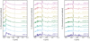 |
Fig. 9. Spectral montage for our set of models at 2.1 d (left panel), 25.7 d (center panel), and 97.8 d (right panel) after explosion (i.e., around the time of bolometric maximum). Each spectrum has been normalized and shifted (a tickmark gives the zero-flux level for each spectrum). The vertical dashed line locates the rest wavelength of Hα and reveals the blue shift of the emission peak at earlier times and higher explosion energies. |
6. Evolution of spectral properties
Figure 9 shows the spectra for our set of models at 2.1, 25.7, and 97.8 d after explosion. The first striking property is that all model spectra look nearly identical (at a given epoch) apart from the difference in line widths. The Hα line profile always reveals a clear P-Cygni profile with very little structure (see also the bottom panel of Fig. 10). In all models (and thus for a range of 56Ni mass and mixing), He I 5875 Å is predicted for up to about 2 d even with a helium mass fraction in the outer ejecta of 0.27. Producing this line requires a non-LTE treatment, as was already obtained and discussed in Dessart & Hillier (2005) – in contrast, Eastman & Kirshner (1989) required an unrealistically large helium mass fraction (of about 0.9) to reproduce this line. Si II 6355 Å causes a blueshifted kink in model a2 at 2.1 d. In general, Ba II 6496.9 Å does not impact Hα, even in the low-energy model a2. In contrast, Ba II 6496.9 Å is very strong in the model X of Lisakov et al. (2017) for SN 2008bk, and indeed causes strong features on top of Hα in all low-energy SNe II-P (Roy et al. 2011; Lisakov et al. 2017, 2018). The multiplet line O I 7774 Å is present in all our models after a few days (this line should not be mistaken at late times with the doublet K I 7665–7699 Å). During the recombination phase, the spectrum evolves little, except for the progressive reddening of the SED and the narrowing of line profiles (see middle and right panels of Fig. 9).
The Hα line is strong and broad at all times in all our models, even for low 56Ni mass or mixing. A similar result was already obtained in Dessart & Hillier (2010), who argued that time dependence is key for reproducing this feature. Mitchell et al. (2001) argued that 56Ni mixing and the associated non-thermal effects are key to reproduce Balmer lines as soon as 4 d after explosion in SN 1987A. But in the simulations of Dessart & Hillier (2010), Balmer lines are strong for 20 d (the time coverage of the models) even though non-thermal effects were not treated at the time in CMFGEN. In the present simulations as well as in Dessart & Hillier (2010), the influence of 56Ni is negligible both for the light curve and for the spectra at these early times.
The Hα emission component, whose wavelength at maximum has a significant blue shift early on, exhibits no obvious skewness (beyond that expected for a P-Cygni profile). The Hα emission flux appears stronger than the absorption part, and stronger than any other line in the optical spectrum. These properties are expected for a spherically-symmetric smooth ejecta in which the spectrum formation region recedes slowly and monotonically through a monotonically increasing density profile.
Figure 10 shows the Doppler velocity at which the location of maximum absorption occurs in Hα and Fe II 5169 Å. These measurements are, at best, indicative of the expansion rate because different lines often show very different width, and often the width of the absorption is very different from the width of the emission (see Sect. 8). It confirms what Fig. 9 illustrates in that each model shows a continuous and monotonic evolution from large to small Doppler velocities. For models that differ in ejecta kinetic energy, the trajectories do not cross. In other words, an offset (of the same sign and relative magnitude) always remains between models of different energy (here the ejecta mass is roughly the same in all models). A weaker 56Ni mixing leads to narrower Hα and Fe II lines for the same kinetic energy (compare models a3 and a3m), but the offset is only sizable at late times when non-thermal processes are strong at the photosphere. The width of Hα (whether in absorption or in emission) remains large even at nebular times (thus even when a photosphere no longer exists) because of the combined effects of ionization freeze-out and non-thermal effects (which may strengthen in the outer ejecta as the γ-ray mean free path increases). At nebular times, Hα forms over a large volume of the ejecta, spanning from the inner regions and going nearly all the way to the maximum ejecta velocities.
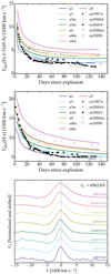 |
Fig. 10. Top panel: doppler velocity at maximum absorption in Fe II 5169 Å for our set of models. We also overplot our measurements for Type II-pec SNe 1987A, 2000cb, 2006V, 2006au, and 2009E. Middle panel: same as top, but now for Hα. A gaussian smoothing with a width of 10–20 Å is used for noisy spectra or when the Hα suffers from strong overlap (e.g., for SN 2006au). In the latter case, the measurement is merely indicative. Bottom panel: montage of spectra for our set of models showing the Hα line profile in Doppler-velocity space at about 200 d after explosion. |
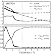 |
Fig. 11. Photospheric structure at 73.5 d after explosion for model a4. Top panel: temperature, the Rosseland-mean opacity, and the Rosseland-mean optical depth. The dashed lines help visualize the location of the photosphere (determined using the Rosseland-mean opacity). Bottom panel: evolution of the gray mean intensity and the gray flux (scaled by r2, where r is the local radius, and subsequently normalized) computed by CMFGEN. |
Observations (overplotted in the top two panels of Fig. 10) reveal a very chaotic behavior. SN 2000cb is the only SN in the sample for which the Hα evolution is compatible with one model (i.e., a5). While model a4 matches SN 1987A early on, the two progressively diverge and beyond 30 d, it is the least energetic ejecta model a2 that corresponds the most closely to SN 1987A. For SN 2006V, the closest match is model a3 (intermediate ejecta energy between models a2 and a4) while its brightness at maximum is the greatest of all SNe II-pec in our sample, and greater than any of our models. This seems in conflict with the notion that stronger Type II SN explosions generally produce a greater amount of 56Ni (Hamuy 2003; Sukhbold et al. 2016; Müller et al. 2017).
As we discuss further below and in Sect. 9, the differences with our model predictions are probably indicative, in part, of departures from spherical symmetry, the presence of clumping or of chemical inhomogeneities, and perhaps of a diversity of power sources at the origin of the SN luminosity. Variation in progenitor radius, mass, and metallicity may also play a part.
7. Photospheric structure at the recombination epoch
Figure 11 shows the photospheric structure of model a4 at 73.5 d after explosion (hence during the recombination epoch and close to bolometric maximum). This structure, which is characteristic of all our models at the recombination epoch, shows that the location of the photosphere (given by the intersection of the two dashed lines) is outside of the H-recombination front, which is where all curves show a jump. The jump in opacity is related to the jump in electron density across the recombination front, and causes the jump in optical depth at ∼2200 km s−1. This jump in optical depth is about 1000 km s−1 deeper than the photosphere and causes the jump in mean intensity and flux. The flux progressively increases from the front and is nearly maximum at the photosphere.
The radius or velocity offset between the location of the recombination front and the location of the photosphere arises from the partial ionization of the gas above the photosphere. This ionization freeze-out is caused by a time-dependent effect (Utrobin & Chugai 2005; Dessart & Hillier 2008).
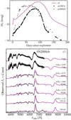 |
Fig. 12. Top panel: absolute V-band light curves for SN 2000cb together with the results for model a5 (we also add SN 1987A). Bottom panel: multiepoch spectra for models a5 compared with the observed spectra of SN 2000cb. The model is redshifted and reddened (see Sect. 2). At each epoch, the spectra are normalized (in this case at 6000 Å) and then shifted vertically. The label ΔMV gives the V-band magnitude difference between observations and model at each time (whenever we can interpolate between photometric data points). |
The temperature profile above the recombination front is very flat, and shows no jump across the photosphere. The Rosseland-mean opacity in these regions does not drop below 0.01 cm2 g−1 (in our simulations, this opacity even increases outwards because the temperature rises outwards, probably because of non-thermal (decay) heating at low density). In CMFGEN, the temperature (together with all level populations) results from balancing the cooling rates and the heating rates while requesting charge neutrality. The temperature structure in regions of optical depth less than about ten (i.e., from below the photosphere and beyond) is very different from the one that would result from the flux-limited-diffusion (FLD) approach often used in radiation hydrodynamics codes (which assume LTE for the gas, and infer the flux from the gradient of the mean intensity or the Planck function; see, e.g., Mihalas & Mihalas 1984). Consequently, the FLD flux computed from such a temperature structure looks unphysical (irrespective of the choice of flux limiter). For example, the optically-thin regions where the non-LTE temperature profile is flat would give a zero flux in FLD while the (total) flux in CMFGEN drops as 1/r2 in spite of this temperature structure (see Fig. 11). In FLD, the temperature must decrease through the photosphere and above in order to carry the flux to infinity. Although this is expected, this emphasizes the fact that radiation-hydrodynamics codes calculate the emergent flux through a completely different physical reasoning and a completely different set of equations compared to a non-LTE time-dependent radiative transfer code like CMFGEN.
8. Comparison to observations of Type II-pec SNe
In this section, we compare the V-band light curves and multiepoch spectra for the selected sample of observed Type II-pec SNe with results from our model set. For the observations, we use the SN characteristics described in Sect. 2 and summarized in Table 1. Our model set was not designed to reproduce these observations (one obvious offset is seen at nebular times when the decay power for our adopted56Ni mass can be offset from the observed luminosity). So, what we present here is a comparison, using the models to guide our understanding of what may be the origin of these events. We start with observed SNe for which we have models that provide a fair match to the light curve or the spectra. We then turn to SNe II-pec whose properties are harder to reproduce with a BSG star explosion model powered by 56Ni decay.
8.1 Comparison to SN2000cb
Figure 12 compares the V-band light curve (with respect to the time of explosion) and the multiepoch spectra of SN 2000cb with the higher energy explosion model a5. The V-band light curve of SN 2000cb differs from that of the prototypical Type II-pec SN 1987A (see top panel of Fig. 12). Starting at −14.6 mag, it brightens to maximum in only 25 days (this is a bolometric rise, not a color effect), which is more typical of Type I SNe (Conley et al. 2006; Drout et al. 2011). It then stays at the same V-band brightness of about −16.2 mag for about 60 d before declining abruptly and becoming nebular at about 110 d after explosion. Photometrically, our model a5 departs sizably from the behavior observed for SN 2000cb. Model a5 is 0.5 mag brighter at the earliest times, then rises slowly to a maximum of −16.4 mag (0.2 mag brighter than SN 2000cb) at 90 d. The transition to the nebular phase occurs on a similar time scale with the same drop in magnitude. Model a5 is overluminous at nebular times by about 0.5 mag (the 56Ni mass is too high by about 60%).
The offset in brightness is therefore at the level of 0.5 mag at most times, which translates into an offset in luminosity of 60%, or 25% in photospheric radius. Hence, this discrepancy is not so large. Reducing the 56Ni mass to 0.1 M⊙ would probably resolve the discrepancy at and beyond maximum. At earlier times, asymmetry might explain the very fast rise (see Utrobin & Chugai 2011; see below).
Spectroscopically, the agreement is generally good at all times shown (from 4.9 until 155.6 d after explosion) with only a few discrepancies. The worst match is seen at 38.9 d, when the model overestimates the strength and width of Hα, Hβ, and Na I D.
A persistent discrepancy is seen for the Hα profile, which, as discussed in Sect. 6, shows a smooth evolution in all models (i.e., the line narrows in time and remains strong both in absorption and emission). In SN 2000cb, Hα is initially broad, but then appears narrow and weak (i.e., narrower and weaker than in model a5). Subsequently, the line remains broad and strengthens relative to the continuum until the last epoch shown. Apart from the first two epochs, the Hα emission is much broader in the model than in the observations, although the discrepancy weakens at later times. The agreement tends to be better for the absorption component than for the emission component (both in strength and width) – the absorption samples material along the line of sight to the SN, while the emission component arises from a larger volume, including lines of sight that do not intersect the SN photosphere. These Hα discrepancies may be attributed to clumping (Dessart et al. 2018), or asymmetry (Utrobin & Chugai 2011), or both.
Hβ is always present (unlike in SN 1987A or SN 2009E, in which it is absent for many weeks at the recombination epoch; see Sects.8.2 and 8.4). The discrepancies that affect Hα do not seem to affect Hβ, which is well reproduced by the model at all times except at 38.9 d. The same agreement holds for Na I D (absent at the first two epochs, poorly matched at 38.9 d, well matched at later times).
These various levels of agreement highlight one major problem in the inference of the expansion rate (and explosion energy) of SN ejecta. Furthermore, a line may be well fitted in absorption but poorly in emission. There is some arbitrariness in relying on either. A better approach is probably to assess the overall match to the observed spectrum rather than arbitrarily adopting one line.
The red part of the optical range is lacking except in the last observation of SN 2000cb, At that time, the Ca II 7300 Å is observed and model a5 matches the strength well (as we will see below, this is not always the case, as for SN 2009E; Sect. 8.4).
Overall, a better model for this SN may be obtained by adopting a lower 56Ni mass of about 0.1 M⊙, which would probably resolve the discrepancy in the light curve at and beyond maximum. At early times, the faster rise to maximum and the rapid narrowing of the Hα line probably requires asymmetry, as proposed by Utrobin & Chugai (2011). In this context, the explosion energy of SN 2000cb is probably lower than in model a5 (2.46 × 1051 erg), and may even be standard for a core-collapse SN since the bulk of the mass, located at low velocity, would then carry little kinetic energy. The same effect likely impacts the inference for GRB/SNe like 1998bw (Dessart et al. 2017). The ejecta mass of model a5 is 13.10 M⊙, much smaller than the value of 22.3 M⊙ proposed by Utrobin & Chugai (2011). Reducing the 56Ni mass by a factor of two would probably narrow the light curve by 30 d (like in the models a3ni and a3). The rapid rise in model a5 seems hard to reconcile simply with strong mixing, since we already employ strong mixing. It would also require more 56Ni ejected in our direction.
The V-band light curve of SN 2000cb is reminiscent of the morphology obtained for magnetar-powered Type II SNe (Dessart & Audit 2018), although it would require a more slowly-rotating magnetar than employed in that study. Further work is needed to understand this object and resolve the various discrepancies.
8.2 Comparison for SN 1987A
SN 1987A has been and is still extensively studied due to its proximity. Its progenitor was identified as a BSG progenitor star, which is also supported by its long and slow rising light curve to an optical maximum at about 90 d after explosion. Numerous independent observations suggest that the explosion was asymmetric on both small and large scales. From late time observations, evidence that the inner ejecta is clympy and asymmetric comes from radio imaging of molecular emission lines (Abellán et al. 2017), from standard spectroscopy (Fransson & Chevalier 1989; Spyromilio et al. 1990; Li et al. 1993; Jerkstrand et al. 2011, 2012), and from integral field spectroscopy (Kjær et al. 2010). Asymmetry is also suggested from early time observations by the fine-structure in the Hα line profile (Hanuschik et al. 1988), the early-time detection of intrinsic polarization (Hoflich 1991; Jeffery 1991), the direction-dependent spectra of SN 1987A observed through light echoes (Sinnott et al. 2013), or the smooth rising optical brightness and the high-energy radiation observed after about 200 d (see, e.g., Arnett et al. 1989). Despite this evidence, all the radiative-transfer modeling for SN 1987A has been limited to 1-D. Multi-D effects can in some cases be taken into account in a simplistic manner. For example, chemical mixing can be treated in a 1-D model, as done here. We can also investigate the effect of clumping in 1-D, as shown in Dessart et al. (2018). Although inadequate, the assumption of spherical symmetry can help identify the signatures of asymmetry in light curves and spectra.
With this in mind, Fig. 13 compares the V-band light curve (with respect to the time of explosion) and the multiepoch spectra of SN 1987A with model a4 (model a4he is also shown in the top panel). The V-band light curve of model a4 rises slowly from −14.3 mag at 1 d to a maximum at 100 d before turning nebular at 150 d. The evolution of SN 1987A differs. Although it has the same brightness at 1 d as model a4, it rises in only 80 d to a maximum 0.4 mag brighter and turns nebular at 120 d. Model a4he, with its greater He to H abundance ratio, has roughly the same brightening rate as model a4 on the way to maximum, peaks at the same time as SN 1987A but at a fainter magnitude by 0.3 mag. Overall, the light curve morphology of these models is analogous to that of SN 1987A, but with a slower rise to a fainter maximum. Our light curves are overall too broad.
The bottom panel of Fig. 13 shows multiepoch spectra for SN 1987A and for model a4. The agreement is fair at early and late times, but there are discrepancies from about one month until the time of maximum. In the observations at 33.8 d, SN 1987A shows a narrower Hα profile, strong Ba II lines, and no Hβ line. The structure in Hα is reminiscent of what is observed in low-luminosity Type II-P SNe (Roy et al. 2011; Lisakov et al. 2018). In the case of SN 2008bk, CMFGEN predicts that the structure in Hα is caused by overlap with Ba II 6496.9 Å, and that this feature is generally not seen in standard-energy SNe II-P because the lines are broader (for the same reason, the low-energy Type II-pec SN 2009E also shows strong Ba II lines; see Sect. 8.4 and Pastorello et al. 2012). In Dessart et al. (2018), we show that clumping can help reduce the ionization of the gas and enhance the abundance of Ba+. This can boost the Ba II line strength and may cause the peculiar morphology of Hα and the absence of Hβ (which overlaps with Ba II 4899 Å and Ba II 4934 Å). Utrobin & Chugai (2005) proposed that the strong Ba II lines were the results of a time-dependent effect. But we include time dependence in our simulations and do not predict strong Ba II lines here. Increasing the Ba abundance by a factor of five at 35 d does not resolve the problem. It is unlikely that the strong Ba II lines are caused by a generic process like time dependence because this feature is not always seen. In our sample of SNe II-pec, SNe 1987A and 2009E are the only objects that show strong Ba II lines.
Figure 10 shows that the Doppler velocity at maximum absorption in Hα and Fe II 5169 Å initially follows the predictions for model a4 but quickly transitions to resembling the properties for the weakest explosions in our sample. Reducing the 56Ni mixing in our simulations would produce narrower lines, but it would delay the rebrightening (compare model a3 and a3m, or see, e.g., Blinnikov et al. 2000). In Dessart et al. (2018), we argue that ejecta clumping can speed up the recession of the photosphere, boosting the luminosity (and the brightening rate) while at the same time producing narrower line profiles. 56Ni mixing cannot achieve this because it tends to produce broader lines, not narrower lines. Such clumping is fundamentally associated with chemical inhomogeneities and implies ejecta asymmetry. It is unclear whether the explosion energy is also asymmetric (i.e., if the shock-deposited energy varies with angle).
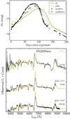 |
Fig. 14. Multiepoch spectra for models a4he compared with the observed spectra of SN 2009mw Takáts et al. (2016). The line profile and color evolutions depart from expectations for a Type II-pec SN: lines are narrower early on; there is no sign of Ca II 7300 Å nor O I 7774 Å; the optical colors are bluer for longer. These features are unlikely to be exclusively a metallicity effect. Some of these features are seen in iPTF14hls (Arcavi et al. 2017). |
Further work is needed to understand the mismatch in light curve properties, in particular the brightening rate to maximum. For the given ejecta mass and explosion energy, a combination of clumping, weaker 56Ni mixing, and a greater helium to hydrogen abundance ratio will probably lead to a satisfactory match with cmfgen. Alternatively, a smaller mass would result in a faster rise to maximum and a brighter peak. Simulations with other codes have yielded a good match to SN 1987A (with parameters that are close to ours; Woosley et al. 1988, Blinnikov et al. 2000; Utrobin et al. 2015), but these use completely different techniques and make very little use of spectral constraints.
8.3 Spectral comparison for SN 2009mw
Figure 14 compares the V-band light curve and the multiepoch spectra of SN 2009mw with model a4he (SN 1987A and model a4 are also shown in the top panel). Although the explosion date is uncertain, SN 2009mw may have had a similar V-band light curve to SN 1987A, with a slower brightening rate to a slightly fainter maximum (Takáts et al. 2016).
Our model a4he has a similar light curve to SN 2009mw, with only slight offsets at the 0.2 mag level (apart from the fall-off from maximum, which occurs about 10 d later in the model – this discrepancy is function of the adopted time of explosion). Spectroscopically, model a4he yields a satisfactory match for the last two epochs shown in Fig. 14, with perhaps a small offset in color (the model is too red). The first spectrum may be inaccurate in relative flux. The Hα profile is not well matched at 15.5 d but is well matched for the last two epochs around the time of maximum. A peculiarity of this SN is the lack of O I 7774 Å and the Ca II doublet at 7300 Å. O I 7774 Å is seen in SN 2006au but not in SN 2006V. The spectral range of our observations for SN 1987A extends to 7200 Å in the optical so no information on O I 7774 Å is accessible for SN 1987A (the spectra of Spyromilio et al. 1991 suggest that O I 7774 Å is also very weak in SN 1987A at the corresponding epochs). Of all SNe II-pec discussed in this paper, SN 2009mw seems the closest analog of SN 1987A, although numerous spectral properties differ (see also discussion in Takáts et al. 2016).
8.4 Comparison for SN 2009E
There is no good model in our set for SN 2009E. Pastorello et al. (2012) presents SN 2009E as a faint clone of SN 1987A but the V-band light curves of these two SNe are in fact very similar (top of Fig. 15). With a reddening E(B − V) of 0.04 mag, the V-band brightness is the same for both at early times, but SN 2009E brightens more slowly (at a rate similar to the rate we obtain in all our models), transitions to the nebular phase about 10 d later. Its nebular-phase brightness suggests it has half the 56Ni mass of SN 1987A, hence about 0.04 M⊙ (Fig. 15; Pastorello et al. 2012). Its decline rate at nebular times is faster, which may indicate γ-ray escape in a lower mass ejecta (unlikely given the narrow lines, which indicate a low expansion rate and a dense inner ejecta). However, this is not a bolometric luminosity plot so this offset may be related to a different evolution of the bolometric correction (the spectra for SNe 2009E and 1987A are evidently different).
Our model a4 (with ejecta kinetic energy of 1.24 × 1051 erg) matches closely the V-band light curve of SN 2009E, with the exception of the larger brightness in the nebular phase. But model a4 is much too energetic for SN 2009E. Even our least energetic model a2 (with ejecta kinetic energy of 0.47 × 1051 erg) overestimates the width of the lines, although the disagreement depends on the choice of line, what part of the line is used, and what 56Ni mixing is adopted (Fig. 16).
The model X of Lisakov et al. (2017), which matches the SN 2008bk spectral evolution, matches closely the spectrum of SN 2009E at 89.5 d (Fig. 16). SN 2009E is thus most likely a low energy explosion, with an expansion rate in the inner ejecta that is much smaller than for SN 1987A. There is no information at early times to constrain how fast the outer ejecta was moving. This spectral comparison also highlights the difficulty of inferring the explosion energy from line profile widths. In Fig. 16, the Ba II line at 6141.7 Å or the Fe II line at 5169 Å has a similar appearance in SNe 2009E and 1987A, as well as model X, while the Hα line profile of SN 2009E is similar to that of model X but considerably narrower and weaker than in SN 1987A. The factor two difference in 56Ni mass between SNe 2009E and 1987A cannot explain the large difference in Hα line strength at bolometric maximum: non-thermal effects for the formation of Hα should be efficient in both. Another peculiarity is that Na I D appears broad in the low energy model X but much narrower in SN 2009E. At 225 d after explosion, model a2 overestimates the strength of the Ca II 7300 Å doublet. This line, which is favored at lower densities relative to the Ca II NIR triplet, is much weaker in SN 2009E than in SN 1987A.
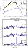 |
Fig. 15. Same as Fig. 12, but now for SN 2009E and model a2 (the top panel also includes SN 1987A and model a4). |
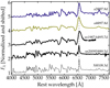 |
Fig. 16. Comparison between the spectra of SN 2009E, SN 1987A, and models a2 and a4 around the time of maximum brightness. We also overplot model X (used to model the low energy Type II-P SN 2008bk; Lisakov et al. 2017) to show that a lower energy than used for model a2 is needed to explain the very narrow Hα. All spectra are normalized and shifted vertically for visibility. Observations were corrected for redshift but not for reddening. |
Overall, SN 2009E is a very peculiar SN with a significant amount of 56Ni (if we assume this is the power source), which allows it to rival the peak brightness of SN 1987A, but with a much lower explosion energy, probably on the order of that for SN 2008bk (see also Pastorello et al. 2012). The binding energy of a BSG star is quite large so a weak explosion should lead to strong fallback, preventing the ejection of 56Ni. One possibility is that the BSG star progenitor is of moderate mass and binding energy, which would cause limited fallback even for a weak explosion. An alternative is that this SN is not powered by 56Ni decay, but perhaps by the compact remnant. The sparse photometric and spectroscopic coverage of SN 2009E does not help resolving this puzzle.
8.5 Spectral comparison for SN 2006V
Figure 17 compares the V-band light curve (with respect to the time of explosion) and the multiepoch spectra of SN 2006V with model a2 (SN 1987A and model a4 are also shown in the top panel). The V-band light curve of SN 2006V shows a long rise to a broad maximum at −17 mag, similar to SN 1987A but brighter by about 1 mag at all recorded epochs. Its color evolution is however much bluer at all times, and the spectra exhibit much narrower lines than in SN 1987A (Taddia et al. 2012).
None of our models match the observed properties of SN 2006V. Compared to SN 1987A (see Fig. 18 for the comparison at ∼30 d), the narrower spectral lines at all times combined with the larger brightness break the expectation that more energetic explosions produce more 56Ni (the adopted reddening is negligible and increasing it would increase the discrepancy). The blue spectra with weak signs of blanketing and narrow lines suggest another power source such as interaction or a central engine (perhaps combined with a metallicity effect). Other spectral anomalies point in this direction. For example, the Hα line profile shows a weak absorption trough (Fig. 18), reminiscent of the interacting SN 1998S in which the cold-dense shell formed during interaction with CSM boosts the Hα emission (Dessart et al. 2016). The lack of O I 7774 Å or the Ca II doublet at 7300 Å is intriguing – this may be an ionization, a density, or an abundance (e.g., metallicity) effect. The last spectrum at 101 d (the exact date depends on the inferred time of explosion but this spectrum is clearly after V-band maximum; Taddia et al. 2012) is very odd for a SN that is about to turn nebular because we can see a strong continuum and no sign of a strengthening line emission.
8.6 Comparison for SN 2006au
Figure 19 compares the V-band light curve and the multiepoch spectra of SN 2006au with model a4 (SN 1987A and model a5 are also shown in the top panel). In the V band, SN 2006au is bright early on, with a magnitude of −16.4 mag (nearly two magnitudes brighter than SN 1987A), rises to a maximum of −16.8 mag in about 70 d (about 15 d earlier than SN 1987A), but then precipitously fades to become very faint, which suggests a very low 56Ni mass. The large brightness and bluer colors early on suggest a bigger progenitor star (say 75−100 R⊙) than for SN 1987A (probably around 50 R⊙) or our present model (Taddia et al. 2012). Models a4 and a5 have a similar brightening rate as SN 2006au prior to maximum, but they peak later and are too bright at nebular times. If the 56Ni mass is very low in SN 2006au, it is not clear what powers the SN at maximum. If we adopt a negligible reddening, the color discrepancy disappears and SN 2006au has a similar brightness to SN 1987A at maximum.
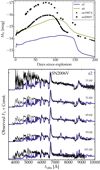 |
Fig. 17. Same as Fig. 12, but now for SN 2006V and model a2 (the top panel also includes model a4 and SN 1987A). SN 2006V deviates strongly from expectations for a 56Ni powered BSG star explosion. |
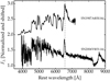 |
Fig. 18. Comparison of the observed optical spectra for SN 1987A and 2006V at about 30 d after the inferred time of explosion. The spectra have been corrected for reddening and redshift, divided by the maximum flux, and shifted. This illustrates the stark color contrast between these two SNe at the same post-explosion phase, as well as the morphological difference in the Hα region (with differences in absorption, strength, width, and overlap with Ba II lines). |
The bottom panel of Fig. 19 shows that model a4 matches some of the spectral properties of SN 2006au, but the model is too red. The observed optical color of SN 2006au is not standard. It has a blue optical color despite the presence of Na I D, Fe II lines, Ti II lines, which are indicative that the spectrum formation region is roughly at the H recombination temperature. The blue color seems to hardly change from 14 to 56 d and the signs of blanketing even seem to weaken. There is no spectroscopic information at nebular times to help constrain the power source and the characteristics of the inner ejecta.
The properties of SNe 2006V and 2006au may in part be driven by a lower metallicity, perhaps much smaller than in the LMC. The problem is that the optical color should eventually redden as the photosphere cools and recedes into the more metal-rich parts of the ejecta. Similarly, a larger radius can yield bluer colors early on, but this effect tends to ebb as the SN progresses through the recombination phase. A power source distinct from radioactive decay might resolve this issue.
SN 2004ek shares some similarities with the properties of SNe 2006V and 2006au (Taddia et al. 2016). It has a similar light curve to SN 2006au (anomalously bright early on), similar narrow lines to SN 2006V (much more narrow than SN 1987A), and a peculiar blue color (peculiar blue colors, narrow lines, and relatively high brightness are also observed in LQS13fn; Polshaw et al. 2016). Its Hα profile shows a weak absorption at the recombination epoch, which is reminiscent of SN 1998S (Dessart et al. 2016). Hence, the peculiar properties of SN 2004ek may reflect the influence of an interaction.
9. Conclusions
We have presented non-LTE time-dependent radiative-transfer simulations for BSG star explosions. We have used one progenitor model to produce a variety of explosion models by varying the energy of the thermal bomb and the prescribed 56Ni mass (in order to correlate the two). We also investigate the effect of a different hydrogen to helium abundance ratio, of a different 56Ni mixing magnitude, as well as of a different 56Ni mass.
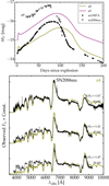 |
Fig. 19. Same as Fig. 12, but now for SN 2006au and model a4 (the top panel also includes model a5 and SN 1987A). |
We use this set of simulations (drawn from a single progenitor model) to compare to observed SNe II-pec. The take-home message from SNe II-pec observations is that there is no prototype for this class. SNe II-pec exhibit a large disparity in optical light curves, optical color curves, in rise time to maximum, in brightness contrast between maximum and the nebular phase, in brightness versus expansion rate. There is also considerable spectral diversity. These events show very distinct line profiles. For example, we see strong Ba II lines in SN 1987A but these lines are weak in SN 2000cb. Additionally, there is strong Hα absorption in SN 1987A while it is weak in SN 2006V. So much diversity is hard to explain, and hard to reproduce with just one set of models. Evidently, explaining Type II-pec SNe requires more than just a reduction in progenitor radius. But our model set helps characterize the incongruous features of SNe II-pec.
Our simulations exhibit a large range in brightness at peak and at nebular times, which correlates with the 56Ni mass. All models (as well as SN 1987A) have a luminosity at peak about 50% greater than the contemporaneous absorbed decay power. For energetic models, γ-ray escape starts soon after maximum and prevents the direct inference of the 56Ni mass. In some models (e.g., a5), the change in IR flux at nebular times compensates for the growing γ-ray escape to yield a decay rate consistent with full γ-ray trapping.
Our models of BSG star explosions powered by 56Ni systematically enter the recombination phase within at most a week after explosion. Subsequently, they evolve at constant color (U – V of about 3 mag), which is also roughly the same for all models in our grid, and their luminosity reflects the trajectory of their (optical) photosphere. Bolometric maximum occurs when the photospheric radius is maximum. Models with a larger explosion energy have a larger photospheric radius at a given post-explosion time and consequently a larger luminosity. This correlation between radius and luminosity no longer holds when clumping is considered (Dessart et al. 2018). In that case, clumping can speed up the recession of the photosphere, yielding smaller photospheric radii but greater luminosities because of the enhanced release of stored radiant energy.
The brightening rate on the rise to maximum brightness is comparable in all our models, except when 56Ni mixing is tuned. Depending on the 56Ni mass, the rise time to maximum lies between 90 and 130 d. At the earliest times, the luminosity is primarily influenced by the explosion energy (we use only one progenitor model, otherwise a dependency on radius and envelope density structure would also appear) and negligibly by the 56Ni mass (even with strong mixing).
The spectral evolution for our model set is very uniform, the only diversity arising from line profile widths (and the indirect effect of line overlap). The greater the initial explosion energy, the broader the line profiles at all times, including at nebular times. At early times, 56Ni plays no role so line broadening is directly related to explosion energy. As the SN enters the recombination phase and the photosphere recedes in mass space, this correlation can break down if 56Ni mixing is changed. For example, a weaker explosion can exhibit broader lines at bolometric maximum if 56Ni is initially more efficiently mixed to large velocities.
We use this set of models to diagnose the properties of observed Type II-pec SNe, in particular to identify, whenever relevant, the signatures of asphericity, clumping, chemical inhomogeneities, mixing, or a distinct power source from decay heating. We find that in all cases our models fail in one way or another to match the observations. This in part reflects the scatter in SNe II-pec properties, in particular the fact that brighter SNe do not necessarily exhibit broader lines at similar epochs. Either the SN luminosity is not powered by 56Ni decay or the correlation between 56Ni mass and explosion energy has a large scatter in Type II-pec SNe.
Photometrically (i.e., in the V band), the best match is obtained for model a4 and SN 2009E, and for a4he and SN 2009mw, while spectrocopically, the best match is obtained for model a5 and SN 2000cb. Photometrically, our models tend to rise too slowly and for too long. This is particularly evident for SNe with a short rise time (25 d for SN 2000cb; 70 d for SN2006au, 80 d for SN 1987A and SN 2006V). Although the data is sparse, the best match is for model a4he and SN 2009mw. The rise time of SN 2009E is matched by model a4, but this model has much broader spectral lines at all times.
In some cases, the mismatch between observations and models is expected. SN 2000cb has a 25 d rise to maximum, which is typical of SNIbc. However, SNe Ibc are characterized by (inferred) ejecta masses of 3–5 M⊙ (see, e.g. Drout et al. 2011). In contrast, our model has an ejecta mass of 13 M⊙ (and a standard explosion energy). The fast rise might indicate that the explosion was asymmetric (Utrobin & Chugai 2011), although in our model sample, even the highest energy models with the highest 56Ni mass have a slower rise to maximum.
SNe2006V and 2006au are too blue at all times to be explained by a standard BSG star explosion. These objects are in tension with 56Ni decay heating. SN 2006V has narrow lines at all times while being the brightest SN II-pec in our sample. SN 2006au is very bright early on, which may suggest a bigger radius than for our adopted progenitor star. But its peculiar color and abrupt fading from maximum are puzzling.
Some of these discrepancies suggest that our progenitors or ejecta models are inadequate. However, in some cases, the colors of both models and observed SNe are in rough agreement and the offset in brightness is associated with offsets in photospheric radii at the 30% level, which is not so large.
Spectroscopically, the comparison between our model set and our selected sample of SNe II-pec is very informative. For SN 2000cb, model a5 matches the whole spectral evolution apart from Hα and one epoch (i.e., at 38.9 d). For SN 1987A, model a4 matches the whole spectral evolution except the phase 20–90 d. During the rise to maximum, the structure of Hα is not matched, and Hβ is predicted but absent. In SN 1987A, the photosphere recedes much faster than in any of our models, showing line widths typical of model a4 initially and of model a2 past 30 d (Fig. 10). The large strength of Ba II lines in SN 1987A is unlikely caused by a time-dependent effect since our simulation treats this process and the Ba II lines are strong only in the model with the lowest explosion energy (a2). Furthermore, Ba II lines are weak in SN 2000cb and SN 2006au. In SN 2009E, Ba II lines are strong and well matched by our model a2. Hence, we believe the strength of Ba II lines is controlled by ionization primarily. Ejecta with a lower expansion rate are denser and produce stronger Ba II lines, as seen in low-energy SNe II-P (Roy et al. 2011; Lisakov et al. 2017, 2018). Clumping can also enhance the Ba II line strength (Dessart et al. 2018).
We find that the width and strength of Hα becomes sensitive to 56Ni decay heating (and the associated non-thermal processes) only after 10–20d. Prior to that, the strength of Balmer lines is sensitive to non-LTE and time-dependent effects.
The blue colors of SNe 2006V and SN2006au might in part be caused by the low metallicity of the SNe II-pec environments. On the modeling side, the mixing we adopt largely erases this low initial metallicity. Allowing for macroscopic mixing without microscopic mixing might perhaps help producing bluer colors. If this chemical segregation and mixing are generic, this notion would not explain why SNe II-pec like 1987A and 2000cb are much redder than other SNe II-pec like 2006V or 2006au. For the latter two (including SN 2004ek; Taddia et al. 2016), a differing powering mechanism might be responsible for the SN brightness.
Understanding the diversity of SNe II-pec will require more work. In the future, we will revisit the present work and cover a more extended parameter space, by including additional progenitor models (mass, radius etc) and a greater variety of explosion characteristics. We also need to consider alternative power sources to decay heating (such as power radiated by the compact remnant and interaction with circumstellar material) as well as investigate the impact of clumping, chemical inhomogeneity, and large-scale asymmetry.
We define the UVOIR flux as the flux falling between 1000 Å and 2.5μm.
Acknowledgments
LD thanks ESO-Vitacura for their hospitality. This work used computing resources of the mesocentre SIGAMM, hosted by the Observatoire de la Côte d’Azur, France.
References
- Abellán, F. J., Indebetouw, R., Marcaide, J. M., et al. 2017, ApJ, 842, L24 [NASA ADS] [CrossRef] [Google Scholar]
- Anderson, J. P., Dessart, L., Gutiérrez, C. P., et al. 2018, Nat. Astron., 2, 574 [NASA ADS] [CrossRef] [Google Scholar]
- Arcavi, I., Howell, D. A., Kasen, D., et al. 2017, Nature, 551, 210 [NASA ADS] [CrossRef] [Google Scholar]
- Arnett, W. D., Bahcall, J. N., Kirshner, R. P., & Woosley, S. E. 1989, ARA&A, 27, 629 [NASA ADS] [CrossRef] [Google Scholar]
- Bionta, R. M., Blewitt, G., Bratton, C. B., Casper, D., & Ciocio, A. 1987, Phys. Rev. Lett., 58, 1494 [NASA ADS] [CrossRef] [PubMed] [Google Scholar]
- Blinnikov, S., Lundqvist, P., Bartunov, O., Nomoto, K., & Iwamoto, K. 2000, ApJ, 532, 1132 [NASA ADS] [CrossRef] [Google Scholar]
- Catchpole, R. M., Menzies, J. W., Monk, A. S., et al. 1987, MNRAS, 229, 15P [NASA ADS] [CrossRef] [Google Scholar]
- Conley, A., Howell, D. A., Howes, A., et al. 2006, AJ, 132, 1707 [NASA ADS] [CrossRef] [Google Scholar]
- Dessart, L., & Audit, E. 2018, A&A, 613, A5 [NASA ADS] [CrossRef] [EDP Sciences] [Google Scholar]
- Dessart, L., & Hillier, D. J. 2005, A&A, 437, 667 [NASA ADS] [CrossRef] [EDP Sciences] [Google Scholar]
- Dessart, L., & Hillier, D. J. 2008, MNRAS, 383, 57 [NASA ADS] [CrossRef] [Google Scholar]
- Dessart, L., & Hillier, D. J. 2010, MNRAS, 405, 2141 [NASA ADS] [Google Scholar]
- Dessart, L., Livne, E., & Waldman, R. 2010a, MNRAS, 405, 2113 [NASA ADS] [Google Scholar]
- Dessart, L., Livne, E., & Waldman, R. 2010b, MNRAS, 408, 827 [NASA ADS] [CrossRef] [Google Scholar]
- Dessart, L., Hillier, D. J., Li, C., & Woosley, S. 2012, MNRAS, 424, 2139 [NASA ADS] [CrossRef] [Google Scholar]
- Dessart, L., Hillier, D. J., Waldman, R., & Livne, E. 2013, MNRAS, 433, 1745 [NASA ADS] [CrossRef] [Google Scholar]
- Dessart, L., Hillier, D. J., Blondin, S., & Khokhlov, A. 2014, MNRAS, 441, 3249 [Google Scholar]
- Dessart, L., Hillier, D. J., Audit, E., Livne, E., & Waldman, R. 2016, MNRAS, 458, 2094 [NASA ADS] [CrossRef] [Google Scholar]
- Dessart, L., John Hillier, D., Yoon, S.-C., Waldman, R., & Livne, E. 2017, A&A, 603, A51 [NASA ADS] [CrossRef] [EDP Sciences] [Google Scholar]
- Dessart, L., Hillier, D. J., & Wilk, K. D. 2018, A&A, 619, A30 [NASA ADS] [CrossRef] [EDP Sciences] [Google Scholar]
- Drout, M. R., Soderberg, A. M., Gal-Yam, A., et al. 2011, ApJ, 741, 97 [NASA ADS] [CrossRef] [Google Scholar]
- Eastman, R. G., & Kirshner, R. P. 1989, ApJ, 347, 771 [NASA ADS] [CrossRef] [Google Scholar]
- Ebisuzaki, T., Shigeyama, T., & Nomoto, K. 1989, ApJ, 344, L65 [NASA ADS] [CrossRef] [Google Scholar]
- Fransson, C., & Chevalier, R. A. 1989, ApJ, 343, 323 [NASA ADS] [CrossRef] [Google Scholar]
- Fryxell, B., Arnett, D., & Mueller, E. 1991, ApJ, 367, 619 [NASA ADS] [CrossRef] [Google Scholar]
- Guillochon, J., Parrent, J., Kelley, L. Z., & Margutti, R. 2017, ApJ, 835, 64 [NASA ADS] [CrossRef] [Google Scholar]
- Hamuy, M. 2003, ApJ, 582, 905 [NASA ADS] [CrossRef] [Google Scholar]
- Hamuy, M., Suntzeff, N. B., Gonzalez, R., & Martin, G. 1988, AJ, 95, 63 [NASA ADS] [CrossRef] [Google Scholar]
- Hanuschik, R. W., Thimm, G., & Dachs, J. 1988, MNRAS, 234, 41P [NASA ADS] [CrossRef] [Google Scholar]
- Hillier, D. J., & Dessart, L. 2012, MNRAS, 424, 252 [NASA ADS] [CrossRef] [Google Scholar]
- Hillier, D. J., & Miller, D. L. 1998, ApJ, 496, 407 [NASA ADS] [CrossRef] [Google Scholar]
- Hirata, K., Kajita, T., Koshiba, M., Nakahata, M., & Oyama, Y. 1987, Phys. Rev. Lett., 58, 1490 [NASA ADS] [CrossRef] [PubMed] [Google Scholar]
- Hoeflich, P. 1988, Proc. Astron. Soc. Aust., 7, 434 [NASA ADS] [CrossRef] [Google Scholar]
- Hoflich, P. 1991, A&A, 246, 481 [NASA ADS] [Google Scholar]
- Jeffery, D. J. 1991, ApJ, 375, 264 [NASA ADS] [CrossRef] [Google Scholar]
- Jerkstrand, A., Fransson, C., & Kozma, C. 2011, A&A, 530, A45 [NASA ADS] [CrossRef] [EDP Sciences] [Google Scholar]
- Jerkstrand, A., Fransson, C., Maguire, K., et al. 2012, A&A, 546, A28 [NASA ADS] [CrossRef] [EDP Sciences] [Google Scholar]
- Kasen, D., & Woosley, S. E. 2009, ApJ, 703, 2205 [NASA ADS] [CrossRef] [Google Scholar]
- Kifonidis, K., Plewa, T., Janka, H.-T., & Müller, E. 2000, ApJ, 531, L123 [NASA ADS] [CrossRef] [PubMed] [Google Scholar]
- Kifonidis, K., Plewa, T., Janka, H.-T., & Müller, E. 2003, A&A, 408, 621 [NASA ADS] [CrossRef] [EDP Sciences] [Google Scholar]
- Kjær, K., Leibundgut, B., Fransson, C., Jerkstrand, A., & Spyromilio, J. 2010, A&A, 517, A51 [NASA ADS] [CrossRef] [EDP Sciences] [Google Scholar]
- Kleiser, I. K. W., Poznanski, D., Kasen, D., et al. 2011, MNRAS, 415, 372 [NASA ADS] [CrossRef] [Google Scholar]
- Kozma, C., & Fransson, C. 1998, ApJ, 496, 946 [NASA ADS] [CrossRef] [Google Scholar]
- Li, C., Hillier, D. J., & Dessart, L. 2012, MNRAS, 426, 1671 [NASA ADS] [CrossRef] [Google Scholar]
- Li, H., McCray, R., & Sunyaev, R. A. 1993, ApJ, 419, 824 [NASA ADS] [CrossRef] [Google Scholar]
- Lisakov, S. M., Dessart, L., Hillier, D. J., Waldman, R., & Livne, E. 2017, MNRAS, 466, 34 [NASA ADS] [CrossRef] [Google Scholar]
- Lisakov, S. M., Dessart, L., Hillier, D. J., Waldman, R., & Livne, E. 2018, MNRAS, 473, 3863 [NASA ADS] [CrossRef] [Google Scholar]
- Liu, W., Dalgarno, A., & Lepp, S. 1992, ApJ, 396, 679 [NASA ADS] [CrossRef] [Google Scholar]
- Livne, E. 1993, ApJ, 412, 634 [NASA ADS] [CrossRef] [Google Scholar]
- Mazzali, P. A., Lucy, L. B., & Butler, K. 1992, A&A, 258, 399 [NASA ADS] [Google Scholar]
- Meaburn, J., Bryce, M., & Holloway, A. J. 1995, A&A, 299, L1 [NASA ADS] [Google Scholar]
- Mihalas, D., & Mihalas, B. W. 1984, Foundations of radiation hydrodynamics (New York: Oxford University Press) [Google Scholar]
- Mitchell, R. C., Baron, E., Branch, D., et al. 2001, ApJ, 556, 979 [NASA ADS] [CrossRef] [Google Scholar]
- Müller, T., Prieto, J. L., Pejcha, O., & Clocchiatti, A. 2017, ApJ, 841, 127 [NASA ADS] [CrossRef] [Google Scholar]
- Pastorello, A., Pumo, M. L., Navasardyan, H., et al. 2012, A&A, 537, A141 [NASA ADS] [CrossRef] [EDP Sciences] [Google Scholar]
- Paxton, B., Bildsten, L., Dotter, A., et al. 2011, ApJS, 192, 3 [Google Scholar]
- Paxton, B., Cantiello, M., Arras, P., et al. 2013, ApJS, 208, 4 [NASA ADS] [CrossRef] [Google Scholar]
- Paxton, B., Marchant, P., Schwab, J., et al. 2015, ApJS, 220, 15 [Google Scholar]
- Phillips, M. M., Heathcote, S. R., Hamuy, M., & Navarrete, M. 1988, AJ, 95, 1087 [NASA ADS] [CrossRef] [Google Scholar]
- Phillips, M. M., Hamuy, M., Heathcote, S. R., Suntzeff, N. B., & Kirhakos, S. 1990, AJ, 99, 1133 [NASA ADS] [CrossRef] [Google Scholar]
- Polshaw, J., Kotak, R., Dessart, L., et al. 2016, A&A, 588, A1 [NASA ADS] [CrossRef] [EDP Sciences] [Google Scholar]
- Roy, R., Kumar, B., Benetti, S., et al. 2011, ApJ, 736, 76 [NASA ADS] [CrossRef] [Google Scholar]
- Schmutz, W., Abbott, D. C., Russell, R. S., Hamann, W.-R., & Wessolowski, U. 1990, ApJ, 355, 255 [NASA ADS] [CrossRef] [Google Scholar]
- Shigeyama, T., & Nomoto, K. 1990, ApJ, 360, 242 [NASA ADS] [CrossRef] [Google Scholar]
- Sinnott, B., Welch, D. L., Rest, A., Sutherland, P. G., & Bergmann, M. 2013, ApJ, 767, 45 [NASA ADS] [CrossRef] [Google Scholar]
- Spyromilio, J., Meikle, W. P. S., & Allen, D. A. 1990, MNRAS, 242, 669 [NASA ADS] [CrossRef] [Google Scholar]
- Spyromilio, J., Stathakis, R. A., Cannon, R. D., et al. 1991, MNRAS, 248, 465 [NASA ADS] [CrossRef] [Google Scholar]
- Sukhbold, T., Ertl, T., Woosley, S. E., Brown, J. M., & Janka, H.-T. 2016, ApJ, 821, 38 [Google Scholar]
- Taddia, F., Stritzinger, M. D., Sollerman, J., et al. 2012, A&A, 537, A140 [NASA ADS] [CrossRef] [EDP Sciences] [Google Scholar]
- Taddia, F., Sollerman, J., Razza, A., et al. 2013, A&A, 558, A143 [NASA ADS] [CrossRef] [EDP Sciences] [Google Scholar]
- Taddia, F., Sollerman, J., Fremling, C., et al. 2016, A&A, 588, A5 [NASA ADS] [CrossRef] [EDP Sciences] [Google Scholar]
- Takáts, K., Pignata, G., Bersten, M., et al. 2016, MNRAS, 460, 3447 [NASA ADS] [CrossRef] [Google Scholar]
- Terreran, G., Pumo, M. L., Chen, T.-W., et al. 2017, Nat. Astron., 1, 228 [Google Scholar]
- Utrobin, V. 1993, A&A, 270, 249 [NASA ADS] [Google Scholar]
- Utrobin, V. P., & Chugai, N. N. 2005, A&A, 441, 271 [NASA ADS] [CrossRef] [EDP Sciences] [Google Scholar]
- Utrobin, V. P., & Chugai, N. N. 2011, A&A, 532, A100 [NASA ADS] [CrossRef] [EDP Sciences] [Google Scholar]
- Utrobin, V. P., Wongwathanarat, A., Janka, H.-T., & Müller, E. 2015, A&A, 581, A40 [NASA ADS] [CrossRef] [EDP Sciences] [Google Scholar]
- Wongwathanarat, A., Janka, H.-T., & Müller, E. 2013, A&A, 552, A126 [NASA ADS] [CrossRef] [EDP Sciences] [Google Scholar]
- Wongwathanarat, A., Mueller, E., & Janka, H.-T. 2015, A&A, 577, A48 [NASA ADS] [CrossRef] [EDP Sciences] [Google Scholar]
- Woosley, S. E. 1988, ApJ, 330, 218 [NASA ADS] [CrossRef] [Google Scholar]
- Woosley, S. E., Pinto, P. A., & Ensman, L. 1988, ApJ, 324, 466 [NASA ADS] [CrossRef] [Google Scholar]
- Yaron, O., & Gal-Yam, A. 2012, PASP, 124, 668 [NASA ADS] [CrossRef] [Google Scholar]
All Tables
Ejecta properties for our model set used as initial conditions for the CMFGEN calculations.
All Figures
|
Fig. 1. Density (top panel) and composition (bottom panel) profiles of our 15 M⊙ model at the onset of core collapse. The model corresponds to a BSG star with a surface radius of 44.8 R⊙. The adopted environment metallicity is 10−7. The bulk of the composition is H and He rich, and the metal-rich part is limited to the He-core below a lagrangian mass of 4 M⊙ (see Sect. 3.1 for discussion). |
| In the text | |
|
Fig. 2. Composition profiles for the inner ejecta of model a2 used in the initial CMFGEN model at 1.1 d (the dashed curve corresponds to 56Ni). The outer ejecta has the same composition as the one at 4000 km s−1. The total ejecta mass for model a2 is 14.30 M⊙. Other models have similar profiles because they all stem from the same progenitor. Differences arise from differences in explosion energy, 56Ni yield, and mixing. Hence, other models show composition profiles that are shifted horizontally (i.e., in velocity space) or vertically (i.e., in yield, which is most relevant for 56Ni, or for H and He in model a4he; see Sect. 3.2 for discussion). |
| In the text | |
|
Fig. 3. Left panel: UVOIR light curves for our CMFGEN simulations, together with the inferred light curve for SN 1987A (the shaded area is bounded by the UVOIR light curves inferred by Catchpole et al. 1987 and Hamuy et al. 1988). Right panel: same as left, but now for the simulations a2, a3, a4, and a5 (which differ primarily in ejecta kinetic energy and 56Ni mass). We also show the total decay power emitted (dashed line) and absorbed (dash-dotted line) for each model. |
| In the text | |
|
Fig. 4. Left panel: same as Fig. 3, but now for the simulations a3, a3m, and a3ni (which differ in chemical mixing magnitude and in 56Ni mass). Right panel: same as left, but now for the simulations a4, a4he, and a4ni (which differ in H/He ratio in the progenitor H-rich envelope and in 56Ni mass). |
| In the text | |
|
Fig. 5. Evolution of the radius, velocity (which can also be deduced directly from the radius and the time elapsed since explosion), and temperature at the photosphere for our set models. The insets in the lower two panels zoom on the epoch around bolometric maximum, when the differences in velocity and temperature between models are harder to discern. |
| In the text | |
|
Fig. 6. Comparison of the V-band light curves for observed SNe II-pec and for our set of models (the time axis corresponds to the time elapsed since V-band maximum; this time is not accurately known given the width of the light curves and the noise in the observed photometry). If we were to use a negligible reddening for SN 2006au (see Sects. 2.4 and 8.6), its optical brightness and color would be comparable to those of SN 1987A. The V-band light curve of SN 2009mw is very similar to that of SN 2009E and thus not shown (Takáts et al. 2016). The SN properties used to make this figure are listed in Table 1. |
| In the text | |
|
Fig. 7. Evolution of the U – V, V – I, and V – H colors for our set of models. |
| In the text | |
|
Fig. 8. Color-color diagram for our set of models. The filled dot indicates the time of bolometric maximum – all models start in the bottom-left corner with a blue optical color. |
| In the text | |
|
Fig. 9. Spectral montage for our set of models at 2.1 d (left panel), 25.7 d (center panel), and 97.8 d (right panel) after explosion (i.e., around the time of bolometric maximum). Each spectrum has been normalized and shifted (a tickmark gives the zero-flux level for each spectrum). The vertical dashed line locates the rest wavelength of Hα and reveals the blue shift of the emission peak at earlier times and higher explosion energies. |
| In the text | |
|
Fig. 10. Top panel: doppler velocity at maximum absorption in Fe II 5169 Å for our set of models. We also overplot our measurements for Type II-pec SNe 1987A, 2000cb, 2006V, 2006au, and 2009E. Middle panel: same as top, but now for Hα. A gaussian smoothing with a width of 10–20 Å is used for noisy spectra or when the Hα suffers from strong overlap (e.g., for SN 2006au). In the latter case, the measurement is merely indicative. Bottom panel: montage of spectra for our set of models showing the Hα line profile in Doppler-velocity space at about 200 d after explosion. |
| In the text | |
|
Fig. 11. Photospheric structure at 73.5 d after explosion for model a4. Top panel: temperature, the Rosseland-mean opacity, and the Rosseland-mean optical depth. The dashed lines help visualize the location of the photosphere (determined using the Rosseland-mean opacity). Bottom panel: evolution of the gray mean intensity and the gray flux (scaled by r2, where r is the local radius, and subsequently normalized) computed by CMFGEN. |
| In the text | |
|
Fig. 12. Top panel: absolute V-band light curves for SN 2000cb together with the results for model a5 (we also add SN 1987A). Bottom panel: multiepoch spectra for models a5 compared with the observed spectra of SN 2000cb. The model is redshifted and reddened (see Sect. 2). At each epoch, the spectra are normalized (in this case at 6000 Å) and then shifted vertically. The label ΔMV gives the V-band magnitude difference between observations and model at each time (whenever we can interpolate between photometric data points). |
| In the text | |
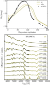 |
Fig. 13. Same as Fig. 12, but now for SN 1987A and models a4 and a4he. |
| In the text | |
|
Fig. 14. Multiepoch spectra for models a4he compared with the observed spectra of SN 2009mw Takáts et al. (2016). The line profile and color evolutions depart from expectations for a Type II-pec SN: lines are narrower early on; there is no sign of Ca II 7300 Å nor O I 7774 Å; the optical colors are bluer for longer. These features are unlikely to be exclusively a metallicity effect. Some of these features are seen in iPTF14hls (Arcavi et al. 2017). |
| In the text | |
|
Fig. 15. Same as Fig. 12, but now for SN 2009E and model a2 (the top panel also includes SN 1987A and model a4). |
| In the text | |
|
Fig. 16. Comparison between the spectra of SN 2009E, SN 1987A, and models a2 and a4 around the time of maximum brightness. We also overplot model X (used to model the low energy Type II-P SN 2008bk; Lisakov et al. 2017) to show that a lower energy than used for model a2 is needed to explain the very narrow Hα. All spectra are normalized and shifted vertically for visibility. Observations were corrected for redshift but not for reddening. |
| In the text | |
|
Fig. 17. Same as Fig. 12, but now for SN 2006V and model a2 (the top panel also includes model a4 and SN 1987A). SN 2006V deviates strongly from expectations for a 56Ni powered BSG star explosion. |
| In the text | |
|
Fig. 18. Comparison of the observed optical spectra for SN 1987A and 2006V at about 30 d after the inferred time of explosion. The spectra have been corrected for reddening and redshift, divided by the maximum flux, and shifted. This illustrates the stark color contrast between these two SNe at the same post-explosion phase, as well as the morphological difference in the Hα region (with differences in absorption, strength, width, and overlap with Ba II lines). |
| In the text | |
|
Fig. 19. Same as Fig. 12, but now for SN 2006au and model a4 (the top panel also includes model a5 and SN 1987A). |
| In the text | |
Current usage metrics show cumulative count of Article Views (full-text article views including HTML views, PDF and ePub downloads, according to the available data) and Abstracts Views on Vision4Press platform.
Data correspond to usage on the plateform after 2015. The current usage metrics is available 48-96 hours after online publication and is updated daily on week days.
Initial download of the metrics may take a while.