| Issue |
A&A
Volume 621, January 2019
|
|
|---|---|---|
| Article Number | A130 | |
| Number of page(s) | 17 | |
| Section | Interstellar and circumstellar matter | |
| DOI | https://doi.org/10.1051/0004-6361/201833612 | |
| Published online | 17 January 2019 | |
Characterising the high-mass star forming filament G351.776–0.527 with Herschel and APEX dust continuum and gas observations★,★★
1
INAF – Osservatorio Astronomico di Cagliari,
Via della Scienza 5,
09047 Selargius (CA),
Italy
e-mail: silvia.leurini@inaf.it
2
Istituto di Astrofisica e Planetologia Spaziali – INAF,
Via Fosso del Cavaliere 100,
00133
Roma,
Italy
3
INAF – Istituto di Radioastronomia, and Italian ALMA Regional Centre,
Via P. Gobetti 101,
40129,
Bologna,
Italy
4
Max-Planck-Institut für Radioastronomie,
Auf dem Hügel 69,
53121
Bonn,
Germany
5
Institute for Astrophysical Research, Boston University,
725 Commonwealth Ave,
Boston,
MA
02215,
USA
6
Centre for Astrophysics and Planetary Science, University of Kent,
Canterbury CT2 7NH,
UK
7
School of Physics, University of New South Wales,
Sydney,
NSW 2052,
Australia
8
European Southern Observatory,
Karl-Schwarzschild-Str. 2,
85748,
Garching bei München,
Germany
9
INAF – Osservatorio Astrofisico di Arcetri,
L.go E. Fermi 5,
50125
Firenze,
Italy
10
Excellence Cluster Universe,
Boltzmannstr. 2,
85748,
Garching bei München,
Germany
Received:
11
June
2018
Accepted:
20
November
2018
G351.776-0.527 is among the most massive, closest, and youngest filaments in the inner Galactic plane and therefore it is an ideal laboratory to study the kinematics of dense gas and mass replenishment on a large scale. In this paper, we present far-infrared and submillimetre wavelength continuum observations combined with spectroscopic C18O (2–1) data of the entire region to study its temperature, mass distribution, and kinematics. The structure is composed of a main elongated region with an aspect ratio of ~23, which is associated with a network of filamentary structures. The main filament has a remarkably constant width of 0.2 pc. The total mass of the network (including the main filament) is ≥2600M⊙, while we estimate a mass of ~2000M⊙ for the main structure. Therefore, the network harbours a large reservoir of gas and dust that could still be accreted onto the main structure. From the analysis of the gas kinematics, we detect two velocity components in the northern part of the main filament. The data also reveal velocity oscillations in C18O along the spine in the main filament and in at least one of the branches. Considering the region as a single structure, we find that it is globally close to virial equilibrium indicating that the entire structure is approximately in a stable state.
Key words: ISM: kinematics and dynamics / ISM: clouds / stars: formation
© ESO 2019
1 Introduction
In recent years increasing evidence has been collected that high-mass star formation is tightly linked to the formation of massive clumps and massive clusters. Observations in molecular tracers (e.g. Schneider et al. 2010; Peretto et al. 2013, 2014; Hacar et al. 2017) have revealed global collapse in several massive clouds and have suggested that clumps build up their mass as a result of the supersonic global collapse of their surrounding cloud. For instance, Peretto et al. (2014) suggested that organised velocity gradients in the filaments of SDC13 are the result of large-scale longitudinal collapse and could generate kinematic support against fragmentation, helping the formation of super-Jeans cores. Also, in the case of DR21, Schneider et al. (2010) detected signs of global collapse of the filament and suggested that its gas content is continuously replenished via sub-filaments. In the case of intermediate-mass clouds, Kirk et al. (2013) identified gas motions onto the filament along defined structures and from the filament onto the central cluster in the Serpens region. Recently, Motte et al. (2018) proposed an evolutionary scenario in which global collapse of massive clouds and hubs generates gas flow streams. In this picture, such flows would efficiently concentrate matter on small scales, helping to increase the mass of low-mass prestellar seeds present in the cloud. With time these seeds eventually become high-mass protostars. Numerical simulations also support this scenario (e.g. Vázquez-Semadeni et al. 2017). Observational evidence of gas streams inflowing on small scales on protostars is reported by Csengeri et al. (2011).
Detailed studies of massive filaments and of their internal structure and dynamics are crucial to better understand the link between high-mass star formation and cloud and cluster formation. Recently, unbiased surveys of the Galactic plane at far-IR and submillimetre wavelengths, namely the APEX Telescope Large Area Survey of the Galaxy (ATLASGAL) and the Herschel infrared Galactic Plane Survey (Hi-GAL; Schuller et al. 2009; Molinari et al. 2010, respectively) have allowed for the compilation of catalogues of candidate filaments over the entire plane (e.g. Li et al. 2016; Wang et al. 2016; Schisano et al. 2018). These studies have shown that massive filaments are in general a few kiloparsec distant (e.g. Li et al. 2016; Schisano et al. 2018). Therefore, high angular resolution observations are needed to resolve linear scales below 0.1–0.2 pc to resolve the kinematics towards individual cores. These catalogues are ideal to select samples of filaments within a few kiloparsecs from the Sun that are suitable for a detailed investigation of the link between massive star formation and cluster formation.
In this paper, we investigate the internal structure of the close-by massive infrared dark cloud (IRDC) G351.776–0.527 (hereafter G351) and that of the network of filaments surrounding this cloud. The study deals with the large-scale filamentary environment of the source, while our previous works (Leurini et al. 2008, 2009, 2011a, 2013, 2014) focussed on the star forming region IRAS 17233–3606 (Clump-1, see Table 1 and Fig. 1). Given the fortuitous proximity of the source (D =0.7–1 kpc, Leurini et al. 2011b, hereafter Paper I; Wienen et al. 2015, and discussion therein), G351 is an ideal target to study a massive filamentary network and its dynamics in detail. The paper is structured as follows. In Sect. 2, we discuss the properties of the source and explain the uniqueness of this laboratory. In Sect. 3, we describe the spectroscopic and continuum observations used in this paper to further characterise G351. In Sect. 4, we study the main properties of G351 and derive its temperature and mass distribution. Section 5 is devoted to the analysis of the gas velocity field. In this section, we demonstrate the velocity coherence of the whole filamentary network, and study the velocity structure of the diffuse/dense gas associated with the source. Finally, we discuss the dynamical state of G351 in Sect. 6.
Clumps in G351.
2 G351.77–0.51: A site of massive star formation
Thanks to Galactic plane surveys at different wavelengths and tracers performed in recent years (e.g. Jackson et al. 2006; Schuller et al. 2009, 2017; Molinari et al. 2010; Burton et al. 2013; Barnes et al. 2015), catalogues of interstellar filaments are now available (e.g. Ragan et al. 2014; Li et al. 2016; Wang et al. 2016; Schisano et al. 2018). These catalogues have shown that massive filaments are on average a few kpc in distance from the Sun: Schisano et al. (2018) found for example that the average mass of Hi-GAL filaments within 3 kpc varies between 200 M⊙ and 800 M⊙ with a binning of 200 pc. Candidates from ATLASGAL are in general more massive given the lower sensitivity of the survey, which is not sensitive to low-mass features, and have an average mass of 470–1700 M⊙ within 3 kpc(in binning of 1 kpc given the low source density, Li et al. 2016).
Despitethe uncertainty in its distance, G351 is the most massive (~ 1300M⊙ for D = 0.7 kpc, Li et al. 2016) and closest filament identified in the ATLASGAL survey of the inner Galactic plane (Li et al. 2016). Compared to close-by massive filaments such as the Orion Integral Filament and NGC 6334 with masses of ~ 10 000–15 000M⊙ (Bally et al. 1987; Tigé et al. 2017) at ~0.4 and 1.7 kpc, respectively (Menten et al. 2007; Russeil et al. 2012), G351 is a younger, less complex object that has only two sites of active massive star formation (Clump-1 and -2, see Table 1 and Fig. 1 and discussion below). The structure is composed by a main elongated region with an aspect ratio of ~ 23 (see Sect. 4.2), which appears nested in a remarkable network of filamentary structures over its whole length (see Fig. 1). In this work we adopt the term branch to refer to these sub-filaments following the naming convention of Schisano et al. (2014). The main filamentary body has been identified as coherent in velocity at vLSR ≈ − 3 km s−1 with a velocity of shift > 1.6 km s−1 between the northern and southern ends (Paper I). Before this work there was no information available on the branches that appear to be connected to the main structure. These structures are seen in extinction at 8 and 24 μm, and they are visible in emission at longer wavelengths in Hi-GAL images for λ ≥ 250 μm (see Fig. 2) and, as a consequence, in the Herschel derived column density map (Schisano et al. 2014).
In Paper I, we analysed the dust continuum emission at 870 μm associated with G351 and identified nine dust clumps (see Table 1 and Fig. 1) with masses ranging between 10 M⊙ and 430 M⊙ depending on the temperature (see Table 4 in Paper I). These clumps are confirmed in the ATLASGAL Gauss clump catalogue (Csengeri et al. 2014) with the exception of Clump-4, which is probably an artefact introduced by CLUMPFIND1 in our previous analysis. The same clumps are also confirmed in the Hi-GAL photometric catalogue (Molinari et al. 2016); roughly another 20 sources are identified in the filamentary network in the region shown in Fig. 1 in at least the 160, 250, and 350 μm Hi-GAL catalogues. We will provide a detailed analysis of the compact sources in a forthcoming paper; in this work we only focus on the massive star formation taking place in G351.
In Paper I, we showed that the majority of the clumps in G351 (Clump-1 for a dust temperature, Tdust, of 35 K, Clump-2 and Clump-5 for Tdust = 25 K, Clump-6, Clump-7, Clump-8, and Clump-11 for 10 K; see Sect. 4.1 for the temperature distribution in the source and Table 4 in Paper I for the masses of the clumps) exceed the threshold for massive star formation determined by Kauffmann & Pillai (2010). At least two clumps (Clump-1 and Clump-3) host active massive star formation. Clump-1 is the brightest submillimetre condensation saturated in Hi-GAL maps (see Fig 2); this clump corresponds to the far-IR source IRAS 17233–3606, and hosts an HII region (Hughes & MacLeod 1993), a hot molecular core (Leurini et al. 2008, 2011a), and a cluster of radio continuum sources (Zapata et al. 2008). Within 10′′ of Clump-3, an HII region has been identified in data taken with the Wide-field Infrared Survey Explorer (WISE; Anderson et al. 2014). Apart from Clump-1, there is little evidence for recently formed high-mass stars in the region. In Table 1, we classify the clumps in G351 according to their far- and mid-IR fluxes as follows: 70 μm weak, when not detected or with weak emission at 70 μm in Hi-GAL (Clump-7 and Clump-11, upper limits F70 μm < 2.5 Jy, and < 2.0 Jy, respectively); mid-IR weak if detected in PACS-70 μm, but with a 21–24 μm flux below 2.6 Jy; and mid-IR bright when the 21–24 μm flux is larger than 2.6 Jy, following the procedure and the classification scheme adopted by König et al. (2017) and Urquhart et al. (2018) for the ATLASGAL catalogues (Contreras et al. 2013; Urquhart et al. 2014; Csengeri et al. 2014). Further evidence of star formation activity is provided by other tracers at several other positions along G351. Four clumps (Clump-1, Clump-2, Clump-3, and Clump-5) show signs of jets and outflows detected in Spitzer IRAC band 3 (see Paper I).
The vicinity of G351, its very early evolutionary phase with only two active sites of massive star formation, and the remarkable filamentary network of branches provide a great opportunity to study the kinematics of dense gas, investigate the mass replenishment from the surrounding environment into sites of massive star formation, and assess the potential for further star formation. In the following discussion, we adopt a distance of 1 kpc for simplicity.
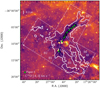 |
Fig. 1 Spitzer 8 μm image of the molecular complex G351. The white contour is 5% of the C18O (2–1) peak intensity (17.6 K km s−1) integrated inthe velocity range − 3.5 ± 0.5 km s−1. The green triangles denote the ATLASGAL clumps identified in Paper I (see Table 1, labelled as C1, C2...). The skeleton of G351 and that of the branches is shown by the white dashed line. The white dotted lines indicate the region observed in CO isotopologues with APEX. The B1–B8 labels indicate the eight branches identified in the |

3 Observations
In this paper we present spectroscopic and continuum observations of the molecular complex G351 at (sub)millimetre wavelengths with the APEX telescope. We complement these data with the Herschel maps from the Hi-GAL survey (Molinari et al. 2010) extracting a region of approximately 0.5° × 0.5° centred on G351 from the flux calibrated maps of the data release version 1 (Molinari et al. 2016). Spitzer 8 and 24 μm data are also used for comparison. A summary of the datasets used in this study is presented in Table 2.
3.1 Spectroscopic observations
The region indicated by white dotted lines in Fig. 1 was mapped in the 13CO and C18O (2–1) transitions with the APEX telescope between August and November 2014. The APEX-1 facility receiver was tuned to a frequency of 218.5 GHz in lower side band (LSB) to observe simultaneously the 13CO (2–1) and C18O (2–1) transitions with a velocity resolution of 0.1 km s−1. The region was covered with three different on-the-fly maps centred on α(J2000) = 17h 26m36.′′47, δ(J2000) = –36°07′43.′′00, α(J2000) = 17h 26m20.′′00, δ(J2000) = −36°15′15.′′30, and α(J2000) = 17h 27m14.′′84, δ(J2000) = −36°08′07.′′70, respectively.This results in a non-uniform noise in the map due to different integration times for the three coverages. For all observations, the position α(J2000) = 17h 26m36.′′47 δ(J2000) = –38°07′43.′′09 was used for sky subtraction after verifying that no 13CO (2–1) emission was detected close to the ambient velocity of the G351 complex (approximately −3 km s−1). Pointing and focus were regularly checked on Mars and on nearby stars (NGC6302, IRAS15194–5115) of the APEX line pointing catalogue2 . For relative calibration, the hot core IRAS 17233–3606 (Leurini et al. 2011a) was regularly observed in the same frequency set-up used for the maps; variations in the 13CO (2–1) line intensity were found to be less than 15%. Data were converted into TMB units assuming a forward efficiency of 0.95 and a beam efficiency of 0.75. Final data cubes were constructed using the CLASS3 gridding routine XY_map, which convolves the data with a Gaussian kernel of one-third of the telescope beam, yielding a final angular resolution slightly coarser than the original beam size. The final spatial resolution of the maps is 30.′′ 2. The average rms in the maps is 0.4 K per velocity channel (0.1 km s−1) with a spread between 0.2 and 0.5 K owing to non-uniform integration time. The region of the map with the higher signal-to-noise ratio covers the main filament and the branches detected in absorption in the mid-IR.
3.2 SABOCA continuum observations
G351 was observed with the APEX telescope in the continuum emission at 350 μm with the Submillimeter APEX Bolometer Camera (SABOCA; Siringo et al. 2010). The observations were performed on 2010 May 7 and 8. The total mapped area is ~ 3.′5 × 11′ orientated along the main filament G351 and covers a smaller area than that of the C18O data. The pointing and focus were checked on SABOCA secondary calibrators sources (G45.1, IRAS 16293) and planets (Uranus and Neptune, also used as primary calibrators)4; the bright hot core IRAS 17233–3606 in the G351 complex was also used as pointing source close to the target. Skydips (fast scans in elevation at constant azimuthal angle) were performed to estimate the atmospheric opacity (τzenith ~ 1.2). The weather conditions at the time of the observations were good with precipitable water vapour levels of 0.3–0.5 mm. The data were reduced with the BOA software (Schuller 2012). We note that the SABOCA data are affected by spatial filtering of extended structures due to the standard data reduction, which relies on the process of correlated noise removal (see for example Belloche et al. 2011, for the LABOCA array). The resolution of the data is 7.′′ 4 with a noise level of 0.9 Jy beam−1.
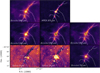 |
Fig. 2 Continuum images of G351 at different wavelengths from 8 μm with Spitzer (bottom left panel) to 870 μm with ATLASGAL-LABOCA. The LABOCA data are affected by filtering of large-scale emission (e.g. Schuller et al. 2009). The solid white line in each panel denotes the skeleton of G351 and of the branches. |
Summary of the datasets available at different wavelengths.
4 Dust and molecular environment of G351
In this section, we discuss the dust continuum emission of G351 (Sect. 4.1), and identify a main body filamentary structure based on the H2 column density distribution (Sect. 4.2). We also investigate the molecular environment of the cloud (Sect. 4.3), and derive the mass distribution of the entire filamentary network (Sect. 4.4) by means of the dust and molecular data.
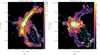 |
Fig. 3 Distribution of the |


4.1 Dust emission
In Fig. 2 we show the continuum emission of the region from 8 to 870 μm using complementary Spitzer and ATLASGAL data. The high resolution of mid-IR Spitzer data (Benjamin et al. 2003; Churchwell et al. 2009; Carey et al. 2009) allow us to distinguish fine details of the filamentary network. In particular, we note several branches in the north giving this region the appearance of a ripped fan. This configuration is seen in several IRDCs and it is expected to appear in models of filaments in global collapse with active environmental accretion onto their structure (Heitsch 2013). The whole filamentary system (including G351 and the network of branches surrounding it) is seen in absorption at 8 and 24 μm. The structure starts to become detected in emission at longer wavelengths. For example, at 70 μm the northern part of G351 is still in absorption against the Galactic background. However, the 70 μm dark region is narrower than at shorter wavelengths and it corresponds to the inner part in absorption at 8 and 24 μm. In the other Hi-GAL maps, G351 and the branches are detected in emission.
The 160–500 μm Hi-GAL data were used to derive a map of the dust temperature and H2 column density,  . We smoothed all data to the beam size of the 500 μm map following a standard approach in the analysis of Herschel data (e.g. Elia et al. 2013, 2017; Schneider et al. 2012). The derived maps have a final resolution of 36′′, which matches very closely that of the spectroscopic data analysed in this paper. To determine the column density and dust temperature, we used a two emission component model (Schisano et al. 2018), in which the fluxes in each pixel at each Herschel band are split between a filament and background component as discussed by Peretto et al. (2010). The background emission is estimated through a linear interpolation over the area of G351 of the fluxes measured around its perimeter. The interpolation direction is aligned perpendicularly to the branches (see Sect. 4). The fluxes are then fit with a modified black-body model, deriving an independent temperature and column density for each component. In both cases, the dust temperature is constrained to be in the range 5–50 K, while no constraint was adopted for the column density estimate. The fluxes were fitted using a modified black-body function as in Elia et al. (2013) and the best fit is found with a χ2 analysis. We assumed a dust opacity law
  with β = 2, ν0 = 1250 GHz, a dust-to-mass ratio of 100, and κ0 = 0.1 cm2 g−1 (Hildebrand 1983) to preserve compatibility with previous works based on other Hi-GAL studies (e.g. Schisano et al. 2014; Elia et al. 2017). Herschel data are saturated at 250 and 350 μm in a region of 25′′ radius centred on Clump-1. Saturated pixels are also detected at 160 and 500 μm around Clump-1 peak position caused by its high brightness. To avoid possible non-linear effects, we masked out a region of radius ~ 30′′ in all Herschel bands before computing Tdust and
  . Nevertheless, the region surrounding Clump-1 peak’s position is affected by larger uncertainties in both quantities. The resulting Tdust and
  distributions of the network are shown in Fig. 3, while the corresponding maps for the background are presented in Appendix A (Fig. A.1).
The main filamentary body of G351 is the denser region of the cloud, which has values exceeding ≥ 3 × 1022 cm−2; the branches, on the other hand, have lower column densities with a maximum value of ~ 1.5 × 1022 cm−2 showing a main difference between the main body and the lower surface brightness shallow surrounding filamentary network. The average column density along the skeleton (see discussion below) is ~ 8.2 × 1022 cm−2 in G351. The dust temperature is distributed differently along the main filament as it is influenced by local star formation. Indeed, the more active southern part (see also Paper I) is warmer with typical temperatures of 27–40 K, reaching the highest values in the surroundings of Clump-1, while the more quiescent northern part has typical temperatures of 11–13 K. The branches in the network have temperatures similar to the northern part of G351.
We derived the spine of G351 and of the network of branches using a twofold approach. For the filamentary network, we made use of the column density map in which the branches have the largest contrast with the surrounding background. However, the resolution of the column density map is 36′′ and with this approach we lose details on the main filament. Therefore, we also computed the skeleton of the main body from the isocontours of the 250 μm continuum emission, which has high signal-to-noise ratio and 18′′ beam size. We adopted the method described by Schisano et al. (2014) and optimised it for the region. The adopted algorithm identifies extended two-dimensional cylindrical-like features based on the analysis of the Hessian matrix of the column density map or the intensity map at 250 μm. We refer to Schisano et al. (2014, 2018) for a detailed discussion of the method. To overcome issues related to the saturation in the Hi-GAL bands, we linearly interpolated the skeleton in the 30′′ in radius masked region. Moreover, we improved the position of the spine by comparing the emission in each of its pixel with that of the direct neighbours. The resulting spine for the entire network is shown in Figs. 1 and 2, while that of the main filament derived from the 250 μm data is shown in Figs. 4 and A.2. In the following analysis, we make use of the spine derived from the column density map only in Sect. 5.1 when we analyse the velocity field along one of the branches.
We identified the main skeleton and additional eight branches in the network. The most prominent are on the south-west of the main IRDC pointing towards the brightest far-IR clumps in the filament, i.e. Clump-1, -2, and -3 (see Table 1); Clump-1 and -3 are also the most evolved in the region. All three branches have a dark counterpart at 8 μm. In the following we label these three sub-filaments as Branch-3, Branch-5, and Branch-6 (Fig. 1). In the south-east of G351 there are two other branches (Branch-2 and -4), which also seem to point to Clump-3 and -1, respectively. Branch-4 is also seen in extinction in the mid-IR. Branch-1 is aligned along the main axis of the central region. Finally, two branches (Branch-7 and -8) are detected in the most northern extension of G351 associated with the fan-like structure seen in the mid-IR.
In the following discussion, we focus on the large-scale dust distribution. The analysis of the dust condensations detected in Hi-GAL and the protostellar content in the filamentary network will be presented in a forthcoming paper (Schisano et al., in prep.).
4.2 Filament main body: G351
By combining the Hi-GAL data (resolution between ~ 10′′ at 70 μm and ~ 36′′ at 500 μm, 0.05–0.17 pc, respectively), which sample the larger scale distribution of the dust, with the SABOCA data (angular resolution ~ 7.′′4, corresponding to 0.04 pc), which trace the innermost high-density region of the filament, we can construct a detailed view of the dust distribution in G351.
We define as the main body of the region the central structure with  cm−2 (corresponding to AV ~ 30; Bohlin et al. 1978; Kauffmann et al. 2017). We also include in the definition two branches, Branch-1 and Branch-8, since they are aligned along the main axis of the central region. All other branches are considered part of the filamentary network.
Based on the column density skeleton, we estimate the length of G351 to be ~ 4.6 pc, assuming an inclination of 0deg against the plane of the sky. This estimate is also confirmed by the Spitzer 8 μm data. Clump-1, the most evolved in G351, is found roughly in the middle of the filament (~ 2.5 pc starting from the northern end) and divides G351 into two parts: the northern part, which is cold and dense, and is clearly detected in emission at far-IR wavelengths and absorption in the mid-IR, and the southern part, which is clearly detected in the dust emission in the far-IR and hosts more evolved sources.
To estimate the width of G351 and determine how it changes along its length, we used the photomotric maps at 350 μm from SABOCA, which have the highest angular resolution among our submillimetre data but filter out the large-scale emission, and at 160 and 250 μm from Hi-GAL, which are sensitive also to the diffuse emission. We selected these two Hi-GAL bands because they have the closest angular resolution (see Table 2) and are close in wavelengths to the SABOCA data. We made the simple hypothesis that the structure is isothermal when estimating the physical width from the photometricmaps. Later we discuss how our results change when dropping this assumption. We divided the maps inseveral regions (see Fig. 4 for the analysis on the SABOCA data and on the 250 μm map) and studied the radial profiles as a function of the distance from the dust skeleton along the length of G351, in particular to investigate variations of its width. The regions have similar lengths of ~ 0.3–0.4 pc along the spine and they are selected to cover the entire length of the main filamentary structure. Results are shown in Figs. 4 and A.2 and in Table 3. The profile of G351 is spatially resolved in all wavelengths adopted for this analysis. The profiles obtained from Hi-GAL are consistently broader than those derived from the SABOCA data, likely because of filtering effects. In the SABOCA data, the width, w, of the filament is well resolved everywhere along the skeleton (see right panel of Fig. 4) with a median value of ~ 0.11 pc and a standard deviation of 0.07 pc. The Hi-GAL profiles are typically 0.2 pc broad (w160 = 0.19 ± 0.05 pc, w250 = 0.21 ± 0.06 pc). The radial profiles for all analysed regions are shown in Fig. A.2 at three wavelengths (350 μm from SABOCA, 250 and 160 μm from Hi-GAL). Interestingly, the width of the filament is essentially constant along its 4.6 pc length for all of the data and all regions, and we do not see any significant deviation from Gaussian shape. Moreover, the widths derived using different Hi-GAL bands are consistent with each other. We also derived the width of the filament using the C18O (2–1) emission integrated in the velocity range − 3.5 ± 0.5 km s−1 (see Sect. 4.3) and found that the width of the diffuse medium associated with G351 is slightly broader ( pc) but also constant along its full extent.
To investigate the impact on our analysis of the assumption that the dust emission is isothermal, we combined our temperature map with the 250 μm thermal continuum emission and derived a column density distribution at 18′′ resolution directly from the 250 μm data (see for example André et al. 2016). We then estimated the width of the filament in the 12 regions described above using the same methodology applied to the photometric maps. Results from both methods are in agreement within the reported errors (Fig. A.3), demonstrating that our assumption of isothermal emission does not influence the results even though the temperature along the filament is not constant. To summarise, the main filamentary body G351 is a structure with an average column density of 8 × 1022 cm−2, an aspect ratio of  , and an almost constant width of ~0.2 pc.
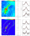 |
Fig. 4 Top panels: Hi-GAL-250 μm map of G351 (left panel). The white solid line indicates the skeleton of the filament obtained from the Hi-GAL data. The map is divided in different regions for the estimate of the filament width along the source. Middle panel: full width at half maximum inarcsec in different regions of the filament. The cross-spine average radial profile of the observed intensity in the Hi-GAL-250 μm data (black thick line, right panel) is given for three regions (a, b, and c; these are also shown in the other two panels) along G351.The solid red line is the Gaussian fit; the thin black line shows the resolution of the data. The error bars show the dispersion of the measurements in the relative region. Bottom panels: as for the top panels but for the SABOCA data. |
4.3 CO isotopologue emission
Figure 5 shows the 13CO (2–1) and C18O (2–1) spectra averaged over the full region mapped with APEX. Figure A.4 shows the distribution of the 13CO emission separately integrated over the velocity intervals of the five different velocity components clearly visible in the integrated 13CO spectrum (peaked around − 24, − 18, − 3.5, + 6, and + 11 km s−1). The weak component at approximately +11 km s−1 is seen mostly in the channel maps since the emission is strongly confined to a small region in the north-west of G351 (see Fig. A.4e). Clearly G351 and the majority of the dark patches seen in extinction in the mid-IR and in emission in the Hi-GAL data belong to the same molecular complex with a typical velocity of approximately − 3 km s−1 (see also Fig. 1). Branch-3, -4, -5, -6, and -8 are detected in both 13CO and C18O, while Branch-2 can be seen only in the 13CO integrated emission map (see Fig. A.4). The other components are not associated with the molecular environment of G351. The emission at approximately − 24 km s−1 is associated with Midcourse Space Experiment (MSX) IRDC G351.64–00.46 (Simon et al. 2006)on the south-west of the main filament (see Fig. A.4). Likely, the 8 μm bright emission on the south of MSX IRDC G351.64–00.46 is associated with the same molecular environment since in Paper I we found CO isotopologue emission centred at approximately − 22 km s−1 at their positions 9, 10, and 12 (see their Fig. 3).
In the following sections, we derive the mass of G351 and of the full network of branches using the dust maps and the C18O (2–1) data (Sect. 4.4), and analyse the velocity field in the structure (Sect. 5) and its dynamical state (Sect. 6). We focus only on the optically thin C18O (2–1) data, avoiding high opacity effects probably affecting the 13CO spectra. Indeed we verified that C18O has low optical depths on the dust condensations in G351 comparing with C17 O (2–1) data from Paper I. The observed ratio of the integrated intensities of C18O to C17 O ranges between 2.4 and 5 under the assumption of opthically thin C17 O emission, implying moderate opacities for C18O of 0.2–0.5 even towards the most massive clumps in G351 and suggesting lower optical depths in the rest of the region.
Width of the G351 filament measured from the average profile in each region and deconvolved for the beam of their corresponding dataset.
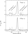 |
Fig. 5 Averaged 13CO (2–1) (top panel) and C18O (2–1) (bottom panel) spectra over the full extent of the APEX map. The dashed lines indicate vLSR of −18, −24, −3.5, +6, and + 11 km s−1. The velocityranges used to obtain the integrated intensity maps shown in Fig. A.4 are also shown. |
4.4 Mass distribution of the filamentary system
We computed the mass of the filament and the network from the Hi-GAL data and from the C18O map assuming thermal equilibrium between dust and gas and using the dust temperature map from Herschel as input to estimate the C18O column density. Around the saturated region we measure a maximum temperature of ~ 30 K. We adopted this value as a lower limit for the effective temperature on Clump-1 given the presence of an HII region and a hot core. This assumption translates into a lower limit to the real mass for the estimate based on C18O. Assuming a CO abundance of 10−4 (Giannetti et al. 2017), a 16O/18O ratio of 58.8Dgc + 37.1 (Wilson & Rood 1994), and a Galactocentric distance, Dgc, equal to 7.4 kpc (Giannetti et al. 2014, revised for d = 1 kpc), the total mass of the system including the network of filaments derived from C18O is ~ 2100M⊙. For the main body ( cm−2), we estimated a mass of ~1200 M⊙. We do however expect higher temperatures close to protostellar sources in particular in the proximity of Clump-1 (see Leurini et al. 2011a). Adopting T =50 K for the saturated region (see Giannetti et al. 2017; Urquhart et al. 2018, for typical temperatures of similar sources at comparable resolutions), the mass estimates based on C18O becomes ~ 2200M⊙ for the whole region and ~ 1300M⊙ for the mainfilament.
We also derived the mass of G351 (~ 1870 M⊙) and that of the whole region including the network (~ 2300 M⊙) using the Hi-GAL column density map. These estimates do not include the saturated region close to Clump-1. Therefore, we also attempted to estimate the mass hosted in the saturated region using the ATLASGAL data assuming a temperature of 30 K as for C18O and the same dust opacity law used for the Hi-GAL data. This assumption leads to a mass of ~ 190M⊙. We note that the values reported in Paper I for the same clump were given for temperatures of 10, 25, and 35 K and for a different opacity law.We finally note that the mass estimate for the network derived from the dust is likely a lower limit due to the difficulty to disentangle the low-contrast branches from the background in a quite extended region of the cloud. Without any background subtraction the total mass of the network including G351 increases to ~ 4560M⊙.
Although the masses based on the dust and on C18O are in good agreement, the C18O estimate for the main structure is lower than that derived from the dust. This could be due to opacity effects and self-absorption in the southern region of G351, where the most massive clumps reside, and to depletion in the youngest and coldest northern part (see Hernandez et al. 2011, for depletion in IRDCs, and Sabatini et al., in prep., for a study of depletion in G351). Also, deviation from the local thermal equilibrium assumption can play a role in this discrepancy.
To summarise, we estimate that the total mass of the network including G351 is between 2600 and 4600 M⊙ including the mass of the saturated region; there is a large uncertainty due to the difficulty to disentangle the low-contrast branches from the background. The main filamentary body has a total mass of 1600–2100 M⊙. Our analysis confirms that the network of branches surrounding G351 harbours a large reservoir of gas and dust which could still be accreted onto the clumps detected along the main filament. This reservoir accounts for about 20% of the total mass if we adopt the estimate of 2600 M⊙ for the network based on the dust and subtracting a background, but increases to up to ~ 60% if no background subtraction is done. Using the C18O data, the mass of the network is ~40% of that of the main substructure.
5 Velocity structure
In this section, we explore the gas kinematics along and across the filament G351 and in the network of branches using the centroid velocity (Vlsr) derived from the C18O emission. In Fig. A.5 we show the C18O channel map emission associated with the region. One can notice that the emission in the southern region is confined within the velocity range [−4.5, −3.4] km s−1, while the northern part emits between − 3.9 km s−1 and − 2 km s−1. This is due to a gradual shift of the C18O emission for the lines of sight from the southern to the northern portion of G351 as can be seen in Fig. 8, where we show the C18O first moment map (see also discussion in Sects. 5.1 and 5.2). This difference invelocity between the northern and southern part was also reported in Paper I based on N2 H+ data. We note that along the spine of G351, C18O is reasonably fit with a single line component except towards IRAS 17233–3606, where optical depth and outflow contamination is evident (Fig. 6). On the other hand, two velocity components are clearly detected in the low-density gas in a large portion of the mapped region (Fig. 7). These two components are also clearly detected in the northern part of G351 in the region from Clump-6 to Clump-7 (see Fig. 9) where a velocity gradient perpendicular to the main axis was detected in the N2 H+ (1–0) data in Paper I (see their Fig. 8). A careful analysis of the isolated hyperfine of the N2 H+ (1–0) line shows that a double-peaked profile is also seen at some positions along the spine of G351 (see Fig. A.6), and we speculate that the previously reported velocity gradient is due to these double velocity components. However, the isolated N2 H+ hyperfine is detected only with low-signal-to-noise ratio and we refrain from a further analysis of these data.
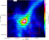 |
Fig. 6 Map of the C18O (2–1) transition overlaid on the integrated emission of the same line in the velocity range [−6, −1] km s−1. The red boxes indicate the regions shown in Fig. 7. |
5.1 Large-scale velocity structure
In Fig. 8 we show the distribution of the first three moments obtained from the C18O (2–1) line in the velocity range [−6, −1] km s−1. The overall velocity distribution of the C18O (2–1) transition is in good agreement with that of N2 H+ presented inPaper I. We confirm the velocity gradient detected in the northern part of G351 and also the gradients detected towards Clump-1 and associated with multiple molecular outflows (e.g. Leurini et al. 2009). Typically, C18O traces lower velocities than N2 H+, but this is expected if N2 H+ is associated with the inner part of the filament and the clumps. We do not detect any clear velocity gradient from the branches towards the dust clumps in the filament although the emission in several branches is systematically red-shifted with respect to the clumps in the main filament (Fig. 8, mid panel). The second moment map (Fig. 8, right panel) shows that the velocity dispersion, σ, is relatively constant along G351 on scales of ~ 30′′ (~ 0.2 pc) with a typical value of ~ 1 km s−1 against thethermal velocity dispersion of ~ 0.2–0.3 km s−1 at a typical (at least in the mid-IR dark part of G351; see Fig. 3) temperature of 10–20 K. This velocity dispersion is also confirmed by the N2 H+ (1–0) data analysed in Paper I (see their Fig. 8). However, the multiple velocity components detected in several C18O spectra (see Sect. 5) could influence the estimate of the velocity moments.
To probe the large-scale velocity distribution, we extract C18O (2–1) spectra along the main axis of the filament, in the perpendicular direction, and along Branch-6 (one of the branches in the network; see Fig. 1) using the skeletons obtained from the 250 μm data and from the H2 column density map after reprojecting them on the C18O data. We then extracted spectra at each position along the three structures (see Figs. 9 and A.7). The individual spectra are analysed in CLASS using the GAUSS fit routine. As noted in the previous section, the C18O data along the spine are well fit with a single velocity component in the majority of the positions. The median dispersion velocity along this direction is ~ 1.1 ± 0.5 km s−1, and this value is not biased by broad profiles associated with active clumps, since it decreases to ~ 1.0 ± 0.1 km s−1 if we exclude the region around Clump-1 and -2. In Fig. 10 we present the velocity field (plotted as velocity centroid against linear distance in arcsec along the spine). In the top panel of Fig. 10, we compare the velocity centroid to the Herschel 500 μm dust brightness, the closest in angular resolution to the APEX observations among the Hi-GAL data. On top of an overall velocity gradient, C18O exhibits a remarkable oscillatory pattern. This pattern is discussed in more detail in Sect. 5.2.
We also investigated the C18O spectra across the width of the main filament. We first selected the most quiescent northern part of G351 and collapsed the data along the direction parallel to the skeleton to increase the signal-to-noise ratio at each position across the spine (Fig. 9). It can be clearly seen that the C18O profiles get narrower at increasing distance from the spine. Moreover, at the outermost positions on the east side of G351 a double-peak profile is detected in the C18O (2–1) line that cannot be resolved in the denser part of G351. We stress that this analysis is performed in the region in which a velocity gradient across the width of G351 is seen in in C18O and N2 H+ (see Fig. 8 and Paper I). It is unlikely that optical depth effects may alter the C18O line profile at the outer positions, since the double peaks are detected in relatively low column density gas (see Fig. 6). Moreover, low opacities are inferred towards the dust clumps by comparison with the C17 O spectra of Paper I (see Sect. 4.3). The spectra shown in Fig. 9 are highly reminiscent of those detected by Peretto et al. (2006) in the intermediate-mass NGC 2264-C clump and interpreted as the results of colliding flows.
Regarding Branch-6 (Fig. A.7), a second velocity component is detected at some positions along its skeleton. The fit results are therefore grouped together using the DBSCAN clustering algorithm5. A crucial input parameter for the algorithm is the number of samples in a neighbourhood for a point to be considered as a core point. We adopt a value of 2 for this parameter, which is equivalent to adopting a “friends of friends” approach such that components that closely follow each other both in position and velocity are grouped together. The clustering results are also sensitive to the maximum distance between two samples for them to be considered as in the same neighbourhood. After testing a range in input parameters, we adopt a parameter set that agrees best with our visual verification. This result in two clusters along the spine of Branch-6: one cluster associated with its full length and a second detected only within a distance of 200′′ from G351 (Fig. 11). As in the case of the spine of G351, the first component, associated with the whole branch, shows an oscillatory pattern on top of an overall velocity gradient of about 1.5 km s−1 over 600′′.
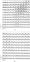 |
Fig. 7 C18O (2–1) spectral map in the two regions denoted with A (panel a) and B (panel b) in Fig. 6. A double-peaked profile is detected at several positions in the low-density gas. |
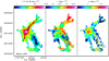 |
Fig. 8 Zeroth (integrated intensity, left panel), first (velocity, middle panel), and second (velocity dispersion, right panel) velocity moments of C18O (2–1) in the velocity range [−6, −1] km s−1. The black squares in the left panel indicate the spine of G351. The white contour in the right panel represents a velocity dispersion of1 km s−1. |
5.2 Velocity structure along the spines
Figure 10 shows the flux density of the 500 μm Hi-GAL data, the centroid line-of-sight velocity of the C18O (2–1) line, and the absolute value of its gradient along the spine of G351 as a function of distance along the spine. The absolute velocity gradient is evaluated over a bin of 0.07 pc. As already noted in Sect. 5.1, velocity fluctuations are detected along the spine of G351 and at least of Branch-6 in C18O (Fig. 11). We also note that on top of a large-scale velocity gradient of about ~ 1 km s−1 pc−1, local velocity gradients are developed close to dust clumps, similar to the findings of Williams et al. (2018) in the massive filamentary hub SDC13.
While we note a general association between the fluctuations and peaks of the velocity gradient and location of dense cores, we donot find a one-to-one correlation. However, all peaks of the velocity gradient are found in within ~ 0.2 pc from dust peaks. Given the typical size of the clumps in G351 (~0.1–0.2 pc, see Table 3 in Paper I), local motions could influence the velocity field in the vicinity of the clumps. Williams et al. (2018) interpreted the correlation between the pattern of the velocity field and the dust peaks as a signature of accretion from the parent filament. However, these velocity variations can have a different interpretation than the steady accretion. For example Smith et al. (2016) found similar velocity shifts in their simulations and determined that they are ascribed to transient motions.
In one of the very few cases where a good agreement between velocity and density peaks has been found (low-mass filament L1571, Hacar & Tafalla 2011), it has been argued that this is a consequence of filament fragmentation via accretion along filaments. These authors modelled such velocity oscillations as sinusoidal perturbations caused by mass inflow along filaments forming cores. Such motions are expected to create a λ∕4 shift between core density and velocity field. As discussed in Henshaw et al. (2014), this applies to an idealistic case. Projection effects can obscure the actual inclination angle of the filament, and thus lead to different velocity signatures. Recent simulations (Heigl et al. 2016; Gritschneder et al. 2017) have started to model the observed velocity oscillations as a natural consequence of filaments that start out in hydrostatic equilibrium and undergo subsonic gravitational fragmentation. Additional effects such as inclination and geometric bents would produce different velocity oscillatory patterns.
Unlike the low-mass filament L1571 in which velocity oscillations have been observed, fluctuations in G351 are highly supersonic. The peak to valley variations in the velocity profile are < 2 km s−1 in either of the two tracers. The free-fall velocity implied for the most massive core in the filament, a 400 M⊙ hot core of radius ~ 0.1 pc (see Tables 3 and 4 of Leurini et al. 2011b) is ~ 6 km s−1. The rotational energy implied by the velocity gradient (see Fig. 10) is negligible compared to the kinetic energy. Therefore, there have to be other factors that significantly influence the gas dynamics. For example, only a fraction of total velocity variation would be identified for a filament inclined at an angle with respect to the observer (Henshaw et al. 2014). Moreover, strong magnetic fields can also significantly slow down accretion (Pillai et al., in prep).
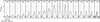 |
Fig. 9 C18O spectra across the main axis of G351 in the most quiescent northern part of the filament. Spectra are collapsed parallel to the main axis. Each spectrum is normalised to its peak intensity value for visualisation. The numbers in each panel indicate the distance from the spine of G351. The label 0′′ denotes the spine. The dashed line indicates a reference velocity of − 3.5 km s−1 (see Fig. 5). |
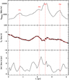 |
Fig. 10 Top panel: distribution of dust brightness from the Hi-GAL-500 μm map (with 36′′ resolution, comparable with that of the line data) as a function of position along the main spine of G351. The starting point for the skeleton is the position α(J2000) = 17h 26m17.′′2, δ(J2000) = −36°02′56.′′7. Labels P1–P4 denote the four peaks detected in the Herschel 500 μm dust brightness and correspond to Clump-5, Clump-2, Clump-1, and Clump-3, respectively. Middle panel: velocity centroid for C18O (2–1) as a function of position along the skeleton of G351. The black squares represent the data points, the red curve obtained by resampling the data over a bin of 15′′ (equivalent to 0.07 pc). Botton panel: absolute velocity gradient along the spine computed over 0.07 pc. |
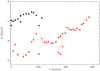 |
Fig. 11 C18O (2–1) velocity centroid as a function of position along the spine of Branch-6. The red and black triangles refer to the two different velocity groups identified by the clustering algorithm. |
6 Dynamical state of G351
In the previous section, we reported that the velocity dispersion in G351 is relatively constant (~ 1 km s−1, see Fig. 8 right panel, and Sect. 5.1) at the resolution of our C18O and N2 H+ observations. However, a double velocity profile is detected in the majority of positions in the low column density gas (Figs. 7 and 9) and we have indications that these double component is also seen along the spine of G351 in the isolated hyperfine of N2 H+ (2–1) (see Fig. A.6). Unfortunately, our data do not allow us to analyse these components in further detail. The median value of the velocity dispersion derived on the spine of G351 from C18O is 1.0 km s−1 (excluding the positions close to Clump-1 and -2). This value is higher than that found in nearby filaments by Arzoumanian et al. (2013); however ourestimate is close to measurements in more massive objects (e.g. Schneider et al. 2010; Mattern et al. 2018). Moreover, we point out that our measurement can be biased by high opacity and dilution effects, which decrease the estimate of  , or by the presence of multiple components.
Using a velocity dispersion of 1 km s−1, we derive a virial mass per unit length 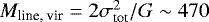 M⊙ pc−1 where σtot is the total velocity dispersion (thermal plus non-thermal) and G the gravitational constant. Considering a total mass of 1600–2100M⊙ for the mainfilament G351 and a length of 4.6 pc (see Sects. 4.1 and 4.4), the mass per unit length, Mline, is 350–450M⊙ pc−1.
The critical mass ratio, Mline∕Mline, vir, of G351 is 0.7–0.9. Given the large uncertainties in the mass estimate, we suggest that G351 is globally in a quasi-stable equilibrium supported by a combination of thermal and turbulent motions. Locally, the cloud may be unstable and collapse. Indeed, we checked the MALT90 (Foster et al. 2011, 2013; Jackson et al. 2013) HCO+, and H13CO+ (1–0) spectra of Clump-1 to look for infall. While the spectra extracted at the position of the dust peak do not show any blue-skewed profiles (see Fig. 2 of Rathborne et al. 2016), the data integrated over a radius of ~ 0.3 pc are suggestive of infall on those scales (see Fig. 12). However, the blue asymmetry in the HCO+ (1–0) disappear on larger scales, indicating local gravitational collapse. This is similar to the findings of Hernandez et al. (2012) who found clear signs of star formation activity, through the presence mid-IR point sources, in gravitationally stable structures.
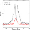 |
Fig. 12 MALT90 HCO+ (1–0) (black line) and H13CO+ (1–0) (red line) spectra of Clump-1 integrated over a radius of ~0.3 pc. |
7 Conclusions
In this paper, we have investigated the temperature and mass distribution of G351.776–0.527 together with the kinematics of moderately dense gas in the region using dust thermal continuum emission maps from APEX and Herschel at different wavelengths and APEX (C18O (2–1)) spectroscopic data. Thanks to the proximity of the source, even the coarse angular resolution of single dish observations allows us to constructa detailed picture of the region. The source consists of a main filamentary structure with a constant width of ~ 0.2 pc and a length of ~4.6 pc surrounded by a complex network of branches seen in absorption at mid-IR wavelengths and in emission in the far-IR. The main filament and network of branches are well separated in H2 column density; there is an average value in the skeleton of G351 of 8.2 × 1022 cm−2 and a maximum of 1.5 × 1022 cm−2 in the network. The most massive dust condensation in G351 seems to divide the main filament in a cold (11–13 K) quiescent northern part and a more active warmer (27–40 K) southern part. The whole region has a mass of at least ~ 2600M⊙, 20% of which is in the branches. Unfortunately, our current dataset does not allow us to understand whether or not there is accretion of material from the branches into G351.
The velocity dispersion of C18O is relativelyconstant along the main filament on scales of ~ 0.2 pc with a typical value of ~ 1 km s−1. C18O is well fit with a single Gaussian component along the spine of G351, but it shows two velocity components in the majority of positions in the low-density gas surrounding G351, and in the branches. Under the assumption that G351 is a single structure, its critical mass ratio is 0.7–0.9. We suggest that G351 is globally in a quasi-stable situation supported by a combination of thermal and turbulent motions close to virial equilibrium, but that locally the filament has become unstable and star formation has started. Finally, we detect velocity fluctuations along the spine of G351 C18O in at least one of the branches of the network in C18O. We also find local velocity gradients close to the dust peaks on top of a large-scale velocity gradient.
Acknowledgements
We thank the anonymous referee for her/his accurate review, which significantly contributed to improving the quality of this paper. We thank Axel Weiss for help with the SABOCA data reduction. E.S. acknowledges financial support from the VIALACTEA Project, a Collaborative Project under Framework Programme 7 of the European Union, funded under Contract #607380. This work was partly supported by the Italian Ministero dell’Istruzione, Università e Ricerca through the grant Progetti Premiali 2012 – iALMA (CUP C52I13000140001), and by the DFG cluster of excellence Origin and Structure of the Universe (www.universe-cluster.de). This work was partially carried out within the Collaborative Research Council 956, subproject A6, funded by the Deutsche Forschungsgemeinschaft (DFG). This research made use of APLpy, an open-source plotting package for Python (Robitaille & Bressert 2012), of Astropy6, a community-developed core Python package for Astronomy (Astropy Collaboration 2013; Price-Whelan et al. 2018), and of Matplotlib (Hunter 2007).
Appendix A Additional material
In this section, we provide additional material. Figure A.1 shows the distribution of the column density and dust temperature for the background component used in the two emission component fit of the Herschel fluxes. Figure A.2 presents the average radial profile of the G351 filament extracted from the photometric images at
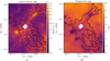 |
Fig. A.1 Distribution of the |

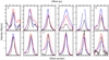 |
Fig. A.2 Average radial profile of G351 estimated from the SABOCA emission at 350 μm emission (solid black line), Hi-GAL-250 μm (red), and Hi-GAL-160 μm data (blue). The panels show the 12 regions of Fig. 4 ordered from top left to bottom right. |
350 μm from SABOCA, and at 250 and 160 μm from Hi-GAL to illustrate how the width of G351 varies along its length. An estimate of the uncertainties introduced in our analysis by our choice of estimating the width of G351 using the photometric images is given in Fig. A.3. Additional information on the velocity field of the region is given in Figs. A.4–A.7.
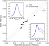 |
Fig. A.3 Comparison between the widths of the 12 regions described in Sect. 4.2 computed on the 250 μm photometric map (y-axis) with those derived on the column density map obtained from the 250 μm Hi-GAL data (x-axis). The widths are not convolved for the beam of the data. In the two panels, the averaged radial profiles for the second (bottom right panel) of Fig. 4 and seventh regions (top left panel) from the bottom are shown derived with both methods. |
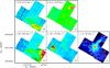 |
Fig. A.4 Integrated emission of the 13CO (2–1) line over five different velocity ranges (see Fig. 5) is shown in colour scale. The point-like emission seen towards Clump-1 in the [+5.6, +6.7] km s−1 and [+9.2, +13.2] km s−1 velocity ranges is due to high-velocity emission associated with molecular outflows (see Leurini et al. 2009). Black contours show the corresponding integrated C18O (2–1) emission from 30% of its peak emission in steps of 30%. The white contours in the bottom right panel show the integrated C18O (2–1) emission in the range − 3.5 ± 0.5 km s−1 from 5 to 45% of the corresponding peak emission in steps of 10%. The B1–B8 labels are as in Fig. 1. |
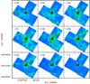 |
Fig. A.5 Channel maps of C18O (2–1). Black contours represent from 10% of the peak intensity of each channel in steps of 10%. The data were smoothed to a spectral resolution of ~0.5 km s−1. |
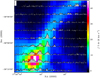 |
Fig. A.6 Map of the N2H+ (1–0) transition overlaid on the integrated emission of the same line in the velocity range [−6, −1] km s−1. |
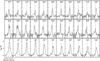 |
Fig. A.7 C18O spectra along Branch-6. The dashed line indicates a reference velocity of − 3.5 km s−1 (see Fig. 5). The numbers in each panel indicate the angular distance from the spine of G351 along the branch. |
References
- Anderson, L. D., Bania, T. M., Balser, D. S., et al. 2014, ApJS, 212, 1 [NASA ADS] [CrossRef] [Google Scholar]
- André, P., Revéret, V., Könyves, V., et al. 2016, A&A, 592, A54 [NASA ADS] [CrossRef] [EDP Sciences] [Google Scholar]
- Arzoumanian, D., André, P., Peretto, N., & Könyves, V. 2013, A&A, 553, A119 [NASA ADS] [CrossRef] [EDP Sciences] [Google Scholar]
- Astropy Collaboration (Robitaille, T. P., et al.) 2013, A&A, 558, A33 [NASA ADS] [CrossRef] [EDP Sciences] [Google Scholar]
- Bally, J., Langer, W. D., Stark, A. A., & Wilson, R. W. 1987, ApJ, 312, L45 [NASA ADS] [CrossRef] [Google Scholar]
- Barnes, P. J., Muller, E., Indermuehle, B., et al. 2015, ApJ, 812, 6 [NASA ADS] [CrossRef] [Google Scholar]
- Belloche, A., Schuller, F., Parise, B., et al. 2011, A&A, 527, A145 [NASA ADS] [CrossRef] [EDP Sciences] [Google Scholar]
- Benjamin, R. A., Churchwell, E., Babler, B. L., et al. 2003, PASP, 115, 953 [NASA ADS] [CrossRef] [Google Scholar]
- Bohlin, R. C., Savage, B. D., & Drake, J. F. 1978, ApJ, 224, 132 [NASA ADS] [CrossRef] [Google Scholar]
- Burton, M. G., Braiding, C., Glueck, C., et al. 2013, PASA, 30, e044 [NASA ADS] [CrossRef] [Google Scholar]
- Carey, S. J., Noriega-Crespo, A., Mizuno, D. R., et al. 2009, PASP, 121, 76 [NASA ADS] [CrossRef] [Google Scholar]
- Churchwell, E., Babler, B. L., Meade, M. R., et al. 2009, PASP, 121, 213 [NASA ADS] [CrossRef] [Google Scholar]
- Contreras, Y., Schuller, F., Urquhart, J. S., et al. 2013, A&A, 549, A45 [NASA ADS] [CrossRef] [EDP Sciences] [Google Scholar]
- Csengeri, T., Bontemps, S., Schneider, N., et al. 2011, ApJ, 740, L5 [NASA ADS] [CrossRef] [Google Scholar]
- Csengeri, T., Urquhart, J. S., Schuller, F., et al. 2014, A&A, 565, A75 [NASA ADS] [CrossRef] [EDP Sciences] [Google Scholar]
- Elia, D., Molinari, S., Fukui, Y., et al. 2013, ApJ, 772, 45 [NASA ADS] [CrossRef] [Google Scholar]
- Elia, D., Molinari, S., Schisano, E., et al. 2017, MNRAS, 471, 100 [NASA ADS] [CrossRef] [Google Scholar]
- Foster, J. B., Jackson, J. M., Barnes, P. J., et al. 2011, ApJS, 197, 25 [NASA ADS] [CrossRef] [Google Scholar]
- Foster, J. B., Rathborne, J. M., Sanhueza, P., et al. 2013, PASA, 30, e038 [NASA ADS] [CrossRef] [Google Scholar]
- Giannetti, A., Wyrowski, F., Brand, J., et al. 2014, A&A, 570, A65 [NASA ADS] [CrossRef] [EDP Sciences] [Google Scholar]
- Giannetti, A., Leurini, S., Wyrowski, F., et al. 2017, A&A, 603, A33 [NASA ADS] [CrossRef] [EDP Sciences] [Google Scholar]
- Gritschneder, M., Heigl, S., & Burkert, A. 2017, ApJ, 834, 202 [NASA ADS] [CrossRef] [Google Scholar]
- Hacar, A., & Tafalla, M. 2011, A&A, 533, A34 [NASA ADS] [CrossRef] [EDP Sciences] [Google Scholar]
- Hacar, A., Alves, J., Tafalla, M., & Goicoechea, J. R. 2017, A&A, 602, L2 [NASA ADS] [CrossRef] [EDP Sciences] [Google Scholar]
- Heigl, S., Burkert, A., & Hacar, A. 2016, MNRAS, 463, 4301 [NASA ADS] [CrossRef] [Google Scholar]
- Heitsch, F. 2013, ApJ, 769, 115 [NASA ADS] [CrossRef] [Google Scholar]
- Henshaw, J. D., Caselli, P., Fontani, F., Jiménez-Serra, I., & Tan, J. C. 2014, MNRAS, 440, 2860 [NASA ADS] [CrossRef] [Google Scholar]
- Hernandez, A. K., Tan, J. C., Caselli, P., et al. 2011, ApJ, 738, 11 [NASA ADS] [CrossRef] [Google Scholar]
- Hernandez, A. K., Tan, J. C., Kainulainen, J., et al. 2012, ApJ, 756, L13 [NASA ADS] [CrossRef] [Google Scholar]
- Hildebrand, R. H. 1983, QJRAS, 24, 267 [NASA ADS] [Google Scholar]
- Hughes, V. A., & MacLeod, G. C. 1993, AJ, 105, 1495 [NASA ADS] [CrossRef] [Google Scholar]
- Hunter, J. D. 2007, Comput. Sci. Eng., 9, 90 [NASA ADS] [CrossRef] [Google Scholar]
- Jackson, J. M., Rathborne, J. M., Shah, R. Y., et al. 2006, ApJS, 163, 145 [NASA ADS] [CrossRef] [Google Scholar]
- Jackson, J. M., Rathborne, J. M., Foster, J. B., et al. 2013, PASA, 30, e057 [NASA ADS] [CrossRef] [Google Scholar]
- Kauffmann, J., & Pillai, T. 2010, ApJ, 723, L7 [NASA ADS] [CrossRef] [Google Scholar]
- Kauffmann, J., Goldsmith, P. F., Melnick, G., et al. 2017, A&A, 605, L5 [NASA ADS] [CrossRef] [EDP Sciences] [Google Scholar]
- Kirk, J. M., Ward-Thompson, D., Palmeirim, P., et al. 2013, MNRAS, 432, 1424 [NASA ADS] [CrossRef] [Google Scholar]
- König, C., Urquhart, J. S., Csengeri, T., et al. 2017, A&A, 599, A139 [NASA ADS] [CrossRef] [EDP Sciences] [Google Scholar]
- Leurini, S., Hieret, C., Thorwirth, S., et al. 2008, A&A, 485, 167 [NASA ADS] [CrossRef] [EDP Sciences] [Google Scholar]
- Leurini, S., Codella, C., Zapata, L. A., et al. 2009, A&A, 507, 1443 [NASA ADS] [CrossRef] [EDP Sciences] [Google Scholar]
- Leurini, S., Codella, C., Zapata, L., et al. 2011a, A&A, 530, A12 [NASA ADS] [CrossRef] [EDP Sciences] [Google Scholar]
- Leurini, S., Pillai, T., Stanke, T., et al. 2011b, A&A, 533, A85 [NASA ADS] [CrossRef] [EDP Sciences] [Google Scholar]
- Leurini, S., Codella, C., Gusdorf, A., et al. 2013, A&A, 554, A35 [NASA ADS] [CrossRef] [EDP Sciences] [Google Scholar]
- Leurini, S., Gusdorf, A., Wyrowski, F., et al. 2014, A&A, 564, L11 [Google Scholar]
- Li, G.-X., Urquhart, J. S., Leurini, S., et al. 2016, A&A, 591, A5 [NASA ADS] [CrossRef] [EDP Sciences] [Google Scholar]
- Mattern, M., Kauffmann, J., Csengeri, T., et al. 2018, A&A, 619, A166 [NASA ADS] [CrossRef] [EDP Sciences] [Google Scholar]
- Menten, K. M., Reid, M. J., Forbrich, J., & Brunthaler, A. 2007, A&A, 474, 515 [NASA ADS] [CrossRef] [EDP Sciences] [Google Scholar]
- Molinari, S., Swinyard, B., Bally, J., et al. 2010, A&A, 518, L100 [NASA ADS] [CrossRef] [EDP Sciences] [Google Scholar]
- Molinari, S., Schisano, E., Elia, D., et al. 2016, A&A, 591, A149 [NASA ADS] [CrossRef] [EDP Sciences] [Google Scholar]
- Motte, F., Bontemps, S., & Louvet, F. 2018, ARA&A, 56, 41 [NASA ADS] [CrossRef] [Google Scholar]
- Peretto, N., André, P., & Belloche, A. 2006, A&A, 445, 979 [NASA ADS] [CrossRef] [EDP Sciences] [Google Scholar]
- Peretto, N., Fuller, G. A., Plume, R., et al. 2010, A&A, 518, L98 [NASA ADS] [CrossRef] [EDP Sciences] [Google Scholar]
- Peretto, N., Fuller, G. A., Duarte-Cabral, A., et al. 2013, A&A, 555, A112 [NASA ADS] [CrossRef] [EDP Sciences] [Google Scholar]
- Peretto, N., Fuller, G. A., André, P., et al. 2014, A&A, 561, A83 [NASA ADS] [CrossRef] [EDP Sciences] [Google Scholar]
- Price-Whelan, A. M., Sip’ocz, B. M., G"unther, H. M., et al. 2018, AJ, 156, 123 [Google Scholar]
- Ragan, S. E., Henning, T., Tackenberg, J., et al. 2014, A&A, 568, A73 [NASA ADS] [CrossRef] [EDP Sciences] [Google Scholar]
- Rathborne, J. M., Whitaker, J. S., Jackson, J. M., et al. 2016, PASA, 33, e030 [NASA ADS] [CrossRef] [Google Scholar]
- Robitaille, T., & Bressert, E. 2012, Astrophysics Source Code Library [record ascl:1208.017] [Google Scholar]
- Russeil, D., Zavagno, A., Adami, C., et al. 2012, A&A, 538, A142 [NASA ADS] [CrossRef] [EDP Sciences] [Google Scholar]
- Schisano, E., Rygl, K. L. J., Molinari, S., et al. 2014, ApJ, 791, 27 [NASA ADS] [CrossRef] [Google Scholar]
- Schisano, E., Molinari, S., Elia, D., Benedettini, M., & Pezzuto, S. 2018, MNRAS, submitted [Google Scholar]
- Schneider, N., Csengeri, T., Bontemps, S., et al. 2010, A&A, 520, A49 [NASA ADS] [CrossRef] [EDP Sciences] [Google Scholar]
- Schneider, N., Csengeri, T., Hennemann, M., et al. 2012, A&A, 540, L11 [NASA ADS] [CrossRef] [EDP Sciences] [Google Scholar]
- Schuller, F. 2012, SPIE Conf. Ser., 8452 [Google Scholar]
- Schuller, F., Menten, K. M., Contreras, Y., et al. 2009, A&A, 504, 415 [NASA ADS] [CrossRef] [EDP Sciences] [Google Scholar]
- Schuller, F., Csengeri, T., Urquhart, J. S., et al. 2017, A&A, 601, A124 [NASA ADS] [CrossRef] [EDP Sciences] [Google Scholar]
- Simon, R., Jackson, J. M., Rathborne, J. M., & Chambers, E. T. 2006, ApJ, 639, 227 [NASA ADS] [CrossRef] [Google Scholar]
- Siringo, G., Kreysa, E., De Breuck, C., et al. 2010, The Messenger, 139, 20 [NASA ADS] [Google Scholar]
- Smith, R. J., Glover, S. C. O., Klessen, R. S., & Fuller, G. A. 2016, MNRAS, 455, 3640 [NASA ADS] [CrossRef] [Google Scholar]
- Tigé, J., Motte, F., Russeil, D., et al. 2017, A&A, 602, A77 [NASA ADS] [CrossRef] [EDP Sciences] [Google Scholar]
- Urquhart, J. S., Csengeri, T., Wyrowski, F., et al. 2014, A&A, 568, A41 [NASA ADS] [CrossRef] [EDP Sciences] [Google Scholar]
- Urquhart, J. S., König, C., Giannetti, A., et al. 2018, MNRAS, 473, 1059 [NASA ADS] [CrossRef] [Google Scholar]
- Vázquez-Semadeni, E., González-Samaniego, A., & Colín, P. 2017, MNRAS, 467, 1313 [NASA ADS] [Google Scholar]
- Wang, K., Testi, L., Burkert, A., et al. 2016, ApJS, 226, 9 [NASA ADS] [CrossRef] [Google Scholar]
- Wienen, M., Wyrowski, F., Menten, K. M., et al. 2015, A&A, 579, A91 [NASA ADS] [CrossRef] [EDP Sciences] [Google Scholar]
- Williams, G. M., Peretto, N., Avison, A., Duarte-Cabral, A., & Fuller, G. A. 2018, A&A, 613, A11 [NASA ADS] [CrossRef] [EDP Sciences] [Google Scholar]
- Wilson, T. L., & Rood, R. 1994, ARA&A, 32, 191 [NASA ADS] [CrossRef] [Google Scholar]
- Zapata, L. A., Leurini, S., Menten, K. M., et al. 2008, AJ, 136, 1455 [NASA ADS] [CrossRef] [Google Scholar]
The CLASS program is part of the GILDAS software package http://www.iram.fr/IRAMFR/GILDAS
All Tables
Width of the G351 filament measured from the average profile in each region and deconvolved for the beam of their corresponding dataset.
All Figures
|
Fig. 1 Spitzer 8 μm image of the molecular complex G351. The white contour is 5% of the C18O (2–1) peak intensity (17.6 K km s−1) integrated inthe velocity range − 3.5 ± 0.5 km s−1. The green triangles denote the ATLASGAL clumps identified in Paper I (see Table 1, labelled as C1, C2...). The skeleton of G351 and that of the branches is shown by the white dashed line. The white dotted lines indicate the region observed in CO isotopologues with APEX. The B1–B8 labels indicate the eight branches identified in the |
| In the text | |
|
Fig. 2 Continuum images of G351 at different wavelengths from 8 μm with Spitzer (bottom left panel) to 870 μm with ATLASGAL-LABOCA. The LABOCA data are affected by filtering of large-scale emission (e.g. Schuller et al. 2009). The solid white line in each panel denotes the skeleton of G351 and of the branches. |
| In the text | |
|
Fig. 3 Distribution of the |
| In the text | |
|
Fig. 4 Top panels: Hi-GAL-250 μm map of G351 (left panel). The white solid line indicates the skeleton of the filament obtained from the Hi-GAL data. The map is divided in different regions for the estimate of the filament width along the source. Middle panel: full width at half maximum inarcsec in different regions of the filament. The cross-spine average radial profile of the observed intensity in the Hi-GAL-250 μm data (black thick line, right panel) is given for three regions (a, b, and c; these are also shown in the other two panels) along G351.The solid red line is the Gaussian fit; the thin black line shows the resolution of the data. The error bars show the dispersion of the measurements in the relative region. Bottom panels: as for the top panels but for the SABOCA data. |
| In the text | |
|
Fig. 5 Averaged 13CO (2–1) (top panel) and C18O (2–1) (bottom panel) spectra over the full extent of the APEX map. The dashed lines indicate vLSR of −18, −24, −3.5, +6, and + 11 km s−1. The velocityranges used to obtain the integrated intensity maps shown in Fig. A.4 are also shown. |
| In the text | |
|
Fig. 6 Map of the C18O (2–1) transition overlaid on the integrated emission of the same line in the velocity range [−6, −1] km s−1. The red boxes indicate the regions shown in Fig. 7. |
| In the text | |
|
Fig. 7 C18O (2–1) spectral map in the two regions denoted with A (panel a) and B (panel b) in Fig. 6. A double-peaked profile is detected at several positions in the low-density gas. |
| In the text | |
|
Fig. 8 Zeroth (integrated intensity, left panel), first (velocity, middle panel), and second (velocity dispersion, right panel) velocity moments of C18O (2–1) in the velocity range [−6, −1] km s−1. The black squares in the left panel indicate the spine of G351. The white contour in the right panel represents a velocity dispersion of1 km s−1. |
| In the text | |
|
Fig. 9 C18O spectra across the main axis of G351 in the most quiescent northern part of the filament. Spectra are collapsed parallel to the main axis. Each spectrum is normalised to its peak intensity value for visualisation. The numbers in each panel indicate the distance from the spine of G351. The label 0′′ denotes the spine. The dashed line indicates a reference velocity of − 3.5 km s−1 (see Fig. 5). |
| In the text | |
|
Fig. 10 Top panel: distribution of dust brightness from the Hi-GAL-500 μm map (with 36′′ resolution, comparable with that of the line data) as a function of position along the main spine of G351. The starting point for the skeleton is the position α(J2000) = 17h 26m17.′′2, δ(J2000) = −36°02′56.′′7. Labels P1–P4 denote the four peaks detected in the Herschel 500 μm dust brightness and correspond to Clump-5, Clump-2, Clump-1, and Clump-3, respectively. Middle panel: velocity centroid for C18O (2–1) as a function of position along the skeleton of G351. The black squares represent the data points, the red curve obtained by resampling the data over a bin of 15′′ (equivalent to 0.07 pc). Botton panel: absolute velocity gradient along the spine computed over 0.07 pc. |
| In the text | |
|
Fig. 11 C18O (2–1) velocity centroid as a function of position along the spine of Branch-6. The red and black triangles refer to the two different velocity groups identified by the clustering algorithm. |
| In the text | |
|
Fig. 12 MALT90 HCO+ (1–0) (black line) and H13CO+ (1–0) (red line) spectra of Clump-1 integrated over a radius of ~0.3 pc. |
| In the text | |
|
Fig. A.1 Distribution of the |
| In the text | |
|
Fig. A.2 Average radial profile of G351 estimated from the SABOCA emission at 350 μm emission (solid black line), Hi-GAL-250 μm (red), and Hi-GAL-160 μm data (blue). The panels show the 12 regions of Fig. 4 ordered from top left to bottom right. |
| In the text | |
|
Fig. A.3 Comparison between the widths of the 12 regions described in Sect. 4.2 computed on the 250 μm photometric map (y-axis) with those derived on the column density map obtained from the 250 μm Hi-GAL data (x-axis). The widths are not convolved for the beam of the data. In the two panels, the averaged radial profiles for the second (bottom right panel) of Fig. 4 and seventh regions (top left panel) from the bottom are shown derived with both methods. |
| In the text | |
|
Fig. A.4 Integrated emission of the 13CO (2–1) line over five different velocity ranges (see Fig. 5) is shown in colour scale. The point-like emission seen towards Clump-1 in the [+5.6, +6.7] km s−1 and [+9.2, +13.2] km s−1 velocity ranges is due to high-velocity emission associated with molecular outflows (see Leurini et al. 2009). Black contours show the corresponding integrated C18O (2–1) emission from 30% of its peak emission in steps of 30%. The white contours in the bottom right panel show the integrated C18O (2–1) emission in the range − 3.5 ± 0.5 km s−1 from 5 to 45% of the corresponding peak emission in steps of 10%. The B1–B8 labels are as in Fig. 1. |
| In the text | |
|
Fig. A.5 Channel maps of C18O (2–1). Black contours represent from 10% of the peak intensity of each channel in steps of 10%. The data were smoothed to a spectral resolution of ~0.5 km s−1. |
| In the text | |
|
Fig. A.6 Map of the N2H+ (1–0) transition overlaid on the integrated emission of the same line in the velocity range [−6, −1] km s−1. |
| In the text | |
|
Fig. A.7 C18O spectra along Branch-6. The dashed line indicates a reference velocity of − 3.5 km s−1 (see Fig. 5). The numbers in each panel indicate the angular distance from the spine of G351 along the branch. |
| In the text | |
Current usage metrics show cumulative count of Article Views (full-text article views including HTML views, PDF and ePub downloads, according to the available data) and Abstracts Views on Vision4Press platform.
Data correspond to usage on the plateform after 2015. The current usage metrics is available 48-96 hours after online publication and is updated daily on week days.
Initial download of the metrics may take a while.