| Issue |
A&A
Volume 619, November 2018
|
|
|---|---|---|
| Article Number | A120 | |
| Number of page(s) | 14 | |
| Section | Interstellar and circumstellar matter | |
| DOI | https://doi.org/10.1051/0004-6361/201732416 | |
| Published online | 13 November 2018 | |
Surround and Squash: the impact of superbubbles on the interstellar medium in Scorpius–Centaurus OB2★
1
Universitäts-Sternwarte München, Ludwig-Maximilians-Universität,
Scheinerstr. 1,
81679
München, Germany
e-mail: This email address is being protected from spambots. You need JavaScript enabled to view it.
2
School of Physical Sciences, University of Tasmania, Hobart, TAS, 7005,
Australia
3
Centre for Astrophysics Research, School of Physics, Astronomy and Mathematics, University of Hertfordshire, College Lane, Hatfield, Hertfordshire AL10 9AB, UK
4
Max-Planck-Institut für extraterrestrische Physik,
Giessenbachstr. 1,
85741 Garching, Germany
5
Excellence Cluster Universe, Technische Universität München,
Boltzmannstrasse 2,
85748 Garching, Germany
6
INAF – Osservatorio Astrofisico di Arcetri,
Largo E. Fermi 5,
50125
Firenze, Italy
Received:
4
December
2017
Accepted:
9
August
2018
Abstract
Context. Feedback by massive stars shapes the interstellar medium and is thought to influence subsequent star formation. The details of this process are under debate.
Aims. We exploited observational constraints on stars, gas, and nucleosynthesis ashes for the closest region with recent massive-star formation, Scorpius–Centaurus OB2, and combined them with three-dimensional (3D) hydrodynamical simulations in order to address the physics and history of the Scorpius–Centaurus superbubble.
Methods. We used published cold gas observations of continuum and molecular lines from Planck, Herschel, and APEX. We analysed the Galactic All Sky Survey (GASS) to investigate shell structures in atomic hydrogen, and used Hipparcos and Gaia data in combination with interstellar absorption against stars to obtain new constraints for the distance to the Hi features. Hot gas is traced in soft X-rays via the ROSAT all sky survey. Nucleosynthesis ejecta from massive stars were traced with new INTEGRAL spectrometer observations via 26Al radioactivity. We also performed 3D hydrodynamical simulations for the Sco–Cen superbubble.
Results. Soft X-rays and a now more significant detection of 26Al confirm recent (≈1 Myr ago) input of mass, energy, and nucleosynthesis ejecta, likely from a supernova in the Upper Scorpius (USco) subgroup. We confirm a large supershell around the entire OB association and perform a 3D hydrodynamics simulation with a conservative massive star population that reproduces the morphology of the superbubble. High-resolution GASS observations reveal a nested, filamentary supershell. The filaments are possibly related to the Vishniac clumping instability, but molecular gas (Lupus I) is only present where the shell coincides with the connecting line between the subgroups of the OB association, suggesting a connection to the cloud, probably an elongated sheet, out of which the OB association formed. Stars have formed sequentially in the subgroups of the OB association and currently form in Lupus I. To investigate the impact of massive star feedback on extended clouds, we simulate the interaction of a turbulent cloud with the hot, pressurised gas in a superbubble. The hot gas fills the tenuous regions of the cloud and compresses the denser parts. Stars formed in these dense clumps would have distinct spatial and kinematic distributions.
Conclusions. The combined results from observations and simulations are consistent with a scenario where dense gas was initially distributed in a band elongated in the direction now occupied by the OB association. Superbubbles powered by massive stars would then repeatedly break out of the elongated parent cloud, and surround and squash the denser parts of the gas sheet and thus induce more star formation. The expected spatial and kinematic distribution of stars is consistent with observations of Sco–Cen. The scenario might apply to many similar regions in the Galaxy and also to active galactic nucleus (AGN)-related superbubbles.
Key words: ISM: kinematics and dynamics / ISM: bubbles / ISM: structure / gamma rays: ISM
© ESO 2018
1 Introduction
The interstellar medium (ISM) is a multifaceted, dynamic place: massive stars inject energy, mass, and freshly synthesised nuclei. This changes its metallicity and sustains multi-phase turbulence with volume-filling, hot and rarefied regions and dense layers compressed by converging flows which may make the transition to the molecular phase and form the next generation of stars (McKee & Ostriker 1977; de Avillez & Breitschwerdt 2005; Heitsch et al. 2008; Hennebelle et al. 2008; Micic et al. 2013; Gómez & Vázquez-Semadeni 2014; Gong & Ostriker 2015). Key drivers of this process are massive stars with their ionising radiation, winds, and core-collapse supernovae.
It is clear that in order to understand these complex phase transitions in the ISM associated with multiple generations of stars, studies at any single wavelength are insufficient. Molecular gas, often associated with ongoing star formation, is best studied at infrared and sub-millimetre wavelengths. Atomic gas is connected with shells pushed out by energy input of young massive stars and efficiently mapped in the 21 cm radio line and with optical absorption against stars. Tenuous gas shock-heated by the winds and explosions of massive stars to keV temperatures is only seen in X-ray observations, and the ejecta themselves can be traced via their radioactive decay lines at MeV energies.
Scorpius–Centaurus OB2 with its associated superbubble (Sco–Cen in the following) is the closest region with clear signs of recent massive-star activity (Preibisch & Mamajek 2008), and is therefore an ideal object to study these effects in detail. The OB association is at a distance of around 140 pc and consists of three subgroups, Upper Scorpius (USco), Upper Centaurus-Lupus (UCL), and Lower Centaurus-Crux (LCC), identified from Hipparcos parallax and proper motion measurements (de Zeeuw et al. 1999; Mel’Nik & Dambis 2009), which has recently been confirmed with Gaia data (Wright & Mamajek 2018). The stellar populations are therefore known in great detail (e.g. de Bruijne 1999; Preibisch et al. 2002; Mamajek et al. 2002). The three sub-groups currently contain many B stars and, given their ages of between 5 and 17 Myr, probably had a number of more massive stars in the past that have already exploded (e.g. de Geus 1992, Table 1 for basic stellar parameters).
With an angular diameter of roughly 90° on the sky, Sco–Cen is also well studied at all wavelengths that carry information about the diffuse ISM (Fig. 1 for a schematic overview). Large area and all-sky surveys, such as the Planck dust maps or the ROSAT all-sky survey (details below), show an essentially post-star-formation region. Most of the molecular gas has been converted to stars, or dislocated into an Hi supershell (Pöppel et al. 2010). The region is a prominent source at keV X-rays (Gaczkowski et al. 2015). As an X-ray bright superbubble, Sco–Cenlikely hosted a supernova explosion within the past million years (Krause & Diehl 2014; Krause et al. 2014). This is consistent with the detection of radioactive 26Al towards one of the subgroups (Diehl et al. 2010).
Causal connection in the observed sequence of star formation events has been suggested (e.g., Preibisch et al. 2002). Preibisch & Zinnecker (2007) detail a triggering scenario for the entire region: star formation first starts in UCL and LCC. Feedback in UCL produces an expanding high-pressure region headed by a shock wave. The shock reached the USco parent cloud about 10 Myr ago, pressurised the cloud and caused the denser parts of the cloud to collapse and form stars. The cloud was subsequently eroded by its internal feedback which caused star formation in nearby clouds, for example, the Lupus I cloud and the ρ Ophiuchus cloud.
Several authors have suggested a possible link between the onset of star formation in the ρ Ophiuchus region and the influence of expanding shells in Sco–Cen: Wilking et al. (1979, 2015) mention magnetic field structure and a higher velocity dispersion of the young stellar objects in the main core of ρ Ophiuchus, which could be a result of the global collapse occurring in the region due to a shock wave from USco (compare also Kwon et al. 2015). Klose (1986) argues for an enhanced gamma ray flux >100 MeV, which he relates to an enhanced level of cosmic ray protons in the region, likely from an energetic explosion which might have played a role in triggering star formation in ρ Ophiuchus. Proper motion studies show that USco has a projected velocity of (μl cosb, μb) = (−24.5, −8.1) mas yr−1 (de Zeeuw et al. 1999). Subtracting this from the projected velocity of the ρ Ophiuchus star cluster, (μl cosb, μb) = (−23.8, −10.7) mas yr−1 (Ducourant et al. 2017), yields a relative motion of (μl cosb, μb) = (0.7, −2.6) mas yr−1. This translates to a projected velocity of 1.7 km s−1 roughly radially away from USco, supporting the connection to feedback in USco.
In a re-analysis of theH IPPARCOS data, Bouy & Alves (2015) have recently expanded on this scenario towards lower Galactic longitudes: they find that the three Sco–Cen subgroups are part of a much larger stream of OB associations and open clusters which form a sequence of star formation over 60 Myr. Star formation would have started 65 Myr ago in the now open cluster NGC 2451A and propagated 350 pc along a filament with the last major episode in USco. Discrete star formation events took place at intervals of a few to 30 Myr.
While the basic case for sequential star formation in Sco–Cen is strong, the details remain poorly understood. For example, if each star formation event sweeps up the dense ISM in its surroundings before it triggers the formation of another OB association in its shell (collect and collapse, e.g. Whitworth et al. 1994), one would expect a monotonic age increase towards the oldest stars, which is not seen in Sco–Cen. This is similar for a distribution of clouds close to equilibrium between self-gravity and pressure that might be triggered to collapse by a passing shock wave. If such a distribution of clouds existed for a time similar to the age of the Sco–Cen stars, one would expect at least some of them to form stars independently of any trigger.
Here, we compile multi-wavelength data on the ISM in Sco–Cen, and interpret these with the help of dedicated superbubble simulations. We find that simple collect and collapse scenarios are disfavoured. Even the smallest, currently star-forming molecular cloud shows evidence for a multi-stage formation process where cloud formation and the onset of star formation are independent from each other. Our simulations show that an initially homogeneous medium cannot fully explain the data. We suggest a multi-stage formation process where the high sound speed in a hot superbubble plays an important role in communicating pressure enhancements to different parts of an initially flattened linear cloud inside the superbubble.
Sco–Cen subgroups and their properties.
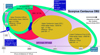 |
Fig. 1 Summary sketch of observational information on the Scorpius–Centaurus region. The OB-association Sco–Cen OB2 has three subgroups of ≈2000 M⊙ each, formed over the last ≈15–20 Myr. Stars are currently forming in the ρ Ophiuchus (moving away from USco at about 1 km s−1) and Lupus I (part of an expanding Hi loop around USco) molecular clouds. See Table 1 for more details on the stars. Hi shells are detected around the youngest OB subgroup, USco, and around the entire region. Diffuse soft X-ray emission is detected towards the superbubble at a level of 1035 erg s−1. One of the detected signatures of massive star winds and supernova explosions is 26Al, towards USco. |
2 Observations and simulations
We summarise observations of dust and molecular gas that have already been discussed in Gaczkowski et al. (2015, 2017), and present new analyses for atomic hydrogen, hot X-ray gas, and gamma rays from the radioactive trace element 26Al. We also performed new 3D hydrodynamics simulations specifically for the Sco–Cen superbubble.
2.1 Molecules and dust
We summarise here our far-infrared and sub-millimetre results for the entire Sco–Cen region including the Lupus I molecular cloud which is placed between the USco and UCL subgroups. Details can be found in Gaczkowski et al. (2015, 2017).
In orderto trace the large-scale dust distribution of the cold dust of the Sco–Cen region we used the archival 850 μm dust map provided by the Planck mission (High Frequency Instrument, Planck legacy archive release PR1 21.03.2013) with a resolution of 5′ (Fig. 2).
The small scale dust observations of the Lupus I molecular cloud were collected in the far-infrared using archival data from Herschel at 70, 160, 250, 350, and 500 μm. The angular resolution was 3.2′′, 4.5′′, 6′′, 8′′, and 11.5′′ in the five maps, respectively (details in Gaczkowski et al. 2015). We obtained 870 μm maps with the LABOCA bolometer at the APEX 12 m telescope with an angular resolution of 19.2′′, and a total field of view of 11.4′ (Gaczkowski et al. 2015, and references therein). Observations along three different scans through the Lupus I cloud in the 13CO(2-1) and C18 O(2-1) lines simultaneously using the APEX-1 receiver obtained a final angular resolution of 30.1′′, which corresponds to 0.02 pc at the distance of Lupus I (140 pc, Gaczkowski 2016; Gaczkowski et al. 2017). Observational results for the Lupus I cloud are summarised in Fig. 3.
Figure 2 shows the 850 μm Planck dust map. The OB-association is located mainly above the galactic plane and is essentially free of dust, as is expected for a star-forming region after a few million years. The remaining cold molecular gas is concentrated in the Lupus I and ρ Ophiuchus clouds and a few filamentary structures. Near ρ Ophiuchus, filaments extend preferentially towards decreasing Galactic longitudes and latitudes. This suggests a large-scale stream of tenuous gas towards the lower left that ablates clouds in this direction, leading to their elongated appearance. Other filaments might be parts of shells of swept-up ISM.
The Lupus I molecular cloud (Fig. 3) is spatially and kinematically associated with an Hi shell around USco, and is located, in projection, on the connecting line between USco and UCL.
The northern part of Lupus I has lower densities, higher temperatures, and no active star formation, while the centre-south part harbours dozens of pre-stellar cores where density and temperature reach their maximum and minimum, respectively. Analysis of the column density probability distribution functions (PDFs) from Herschel data shows double-peaked profiles for all parts of the cloud. We attribute this to an external compression event, after the lognormal PDF had first been established, quite possibly caused by turbulence associated with thin-shell instabilities. Increase of ambient pressure as expected, for example, from a supernova in USco could plausibly have compressed part of the Lupus I cloud and shifted its PDF to higher densities. In those parts with active star formation, the PDFs show a power-law tail. The PDFs we calculated from our LABOCA data trace the denser parts of the cloud showing one peak and a power-law tail. With LABOCA we identified 15 cores with masses between 0.07 and 1.71 M⊙ and a total mass of ≈ 8 M⊙. The mass of the cores represents ≈5% of the total gas and dust mass of the cloud of ≈ 172 M⊙ (average between the Herschel and Planck resulting dust mass).
13CO(2-1) and C18O(2-1) line observations of Lupus I with the APEX telescope at three distinct scans through the cloud show a complex kinematic structure with several line-of-sight components that may overlay each other. Such complex kinematic structure is expected for turbulence. Local-thermodynamic-equilibrium analysis showed that the C18 O line is optically thin almost everywhere within the three scanned regions, in contrast to the 13CO line. We therefore used the C18O measurements to assess the kinematics. The non-thermal velocity dispersion is in the transonic regime in all parts of the cloud. This level of turbulence is expected from instabilities on a decelerating shell (Krause et al. 2013).
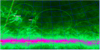 |
Fig. 2 Planck 850 μm dust map of the Scorpius–Centaurus region in Galactic coordinates. The Milky Way plane can be seen as a pink band over the entire image. Scorpius–Centaurus OB2 (green ellipses indicate the location of the three subgroups) is mainly above the plane and is essentially dust-free apart from the ρ Ophiuchus and Lupus I clouds (labelled). Coordinates are Galactic and given in degrees. The colour scale ranges from black (low), through green, pink, red, orange to yellow (high). |
2.2 Atomic gas
We analysed the entire Sco–Cen region in Hi using the Parkes Galactic all-sky survey (GASS; McClure-Griffiths et al. 2009; Kalberla et al. 2010)1. GASS has a spatial resolution of 16.2′ (Kalberla & Haud 2015), which corresponds to a length scale of 0.66 pc at the characteristic distance of Lupus I. The velocity resolution is 1 km s−1. We focused in particular on the prominent shell around USco where the GASS observations reveal finer detail than previous observations (compare Pöppel et al. 2010).
In orderto assess the distances of Hi features, we compared their characteristic velocities with Na-D absorption features measured against stars with known distances. We use catalogued absorption features from Pöppel et al. (2010) and Welsh et al. (2010)2. Distances were calculated from parallax measurements with Hipparcos with distance uncertainties of ≈ 7% for 50–100 pc, and ≈15% for 200–250 pc distances. Where available, more accurate Gaia parallax measurements were used3 (Gaia Collaboration 2016; Lindegren et al. 2016). In the present data release 1, parallax uncertainties are typically 0.3 mas (0.3 mas) for statistical (systematical) uncertainties, which translates to a statistical error of 5% at a distance of 150 pc. For most cases the distance estimation using parallax measurements led to similar results but there are also some cases where the Hipparcos and the Gaia distances show significant differences, for example, the star HD 146284 which has a distance of 264 pc according to the Hipparcos data and 181.23 pc according to the Gaia data. Gaia distances were adopted where available.
We associated Nai lines with Hi features based on the Hi profile and cap line widths at 3 km s−1 to ensure that the line peak is not fitted to a broad Hi component that reflects the galactic disc background. If the Nai absorption line fits more than one Hi component, the closer match is selected.
In this way, we derived upper limits for the distances to Hi features, where a star shows associated absorption, and lower limits where a star shows no associated Nai absorption feature.
We have integrated the Hi data cubes over suitably selected velocity channels and show these integrated channel maps in Fig. 4. These maps show shells and arcs as reported already by Pöppel et al. (2010), as well as high intensity in the Galactic plane. We discern two main features of interest: first, a large supershell surrounding the entire region. It is located in an oblique way with respect to the Galactic plane, at greater latitudes for greater longitudes. This morphology is similar to the one of the Sco–Cen subgroups and encloses them in projection. It is expected that superbubbles within the disc scale height (≈ 150 pc for HI; Narayan & Jog 2002) are oriented randomly with respect to the Galactic disc plane.
The second prominent structure is the USco loop, which we show in more detail in a single-channel map in Fig. 5. The loop plausibly originates from the USco stars. We show its 3D structure with velocity as the third dimension also in Fig. 5. Circles were fitted by eye to the individual channel maps. The loop appears to have roughly constant diameter in all velocity channels, suggesting that it has experienced blow-out into (or away from) the line of sight, and only its cylindrical central parts remain visible.
We have highlighted another loop-like structure in the 3D representation in Fig. 5. This smaller loop is seen towards approaching velocities and towards USco. It could be a signature of erosion of the ISM between the Sco–Cen superbubble and the local superbubble.
For the distances to the Hi features in the Sco–Cen region, we have obtained 14 lower limits and 44 upper limits by associating the Hi features to Nai absorption lines. For clarity, we show only the upper limits in Fig. 4. From a statistical analysis (Fig. 6), we find Hi features at a range of distances, bounded by 100 pc from below and about 250 pc fromabove. The more detailed histogram for distances between 100 and 300 pc shows that we find more lower limits below 150 pc, and more upper limits for above 150 pc. This suggests that the Hi features are located at a range of distances centred around a characteristic value of 150 pc. Because of the distance limit in the Nai database, we can only say that the supershell extends to at least 220 pc. This statistical analysis is consistent with the distances for individual features determined by Pöppel et al. (2010).
Using these distances, we can determine approximate sizes of the Hi features. The big supershell surrounding the entire Sco–Cen region is approximately 90° in diameter, corresponding to 240 pc at a distance of 150 pc. The USco loop is 25° in diameter, which corresponds to 65 pc. The Hi shell itself is spatially resolved and has a thickness of about 4°, corresponding to about 10 pc. It has a filamentary appearance. Thick filamentary shells are expected from 3D simulations of superbubbles that resolve the clumping instabilities in the shell (Krause et al. 2013). The sonic random motions observed in the CO lines in part of the shell (Lupus I, compare Sect. 2.1) would also be expected as a result of the instability. Detailed estimates of unstable wavelengths and timescales are difficult for this case, as the blowout has likely modified the deceleration history of the shell, which is a crucial parameter (e.g. Vishniac & Ryu 1989). We refer to Sect. 3 for further discussion on this topic.
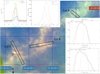 |
Fig. 3 Lupus I molecular cloud: combined image of the mosaics obtained with Spitzer/MIPS at 24 μm (blue), Herschel/PACS at 160 μm (green), and the Herschel/SPIRE at 500 μm (red), all in logarithmic scales. The right overplotted panels show the column density distribution functions of the northern (top panels) and southern (bottom panels) parts of Lupus I and the central panel shows the histograms of the dust temperature in different parts of the cloud (see details in Gaczkowski et al. 2015). Left panel: gas velocity profiles averaged along cuts A, B, and C, which are highlighted by the black boxes. Ecliptic coordinates are used for this figure to help identify northern and southern parts. Galactic coordinates of the centre of Lupus I: l = 338° 50′, b = 16° 40′. |
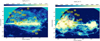 |
Fig. 4 Intensity of the 21 cm line of neutral hydrogen towards Sco–Cen. Left (right) panel: emission integrated between −20 and 0 km s−1 (0 and 10 km s−1). The numbers in the yellow boxes show upper distance limits for the Hi features derived from velocity-matched Nai absorption lines against stars with distances known from parallax measurements by Hipparcos and Gaia. |
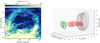 |
Fig. 5 Intensity of the 21 cm line of neutral hydrogen towards USco in the 7.4 km s−1 velocity channel (left panel) and by-eye characterisation of the Hi structures across multiple velocity channels (right panel). Three groups of rings are apparent: the USco loop (black), which corresponds to the dominant loop in the channel map on theleft, and two smaller, tube-like structures (green and red) which are cospatial but separated in velocity space. The red and green rings might be a result of erosion of the Hi interface between the Sco–Cen superbubble and the local bubble, where the hot gas streaming through the hole ablates and accelerates the Hi. |
2.3 Hot gas
The ROSAT all sky survey (Snowden et al. 1997; Max-Planck-Institut für extraterrestrische Physik (MPE) archive) shows X-ray emission from hot plasma in the interiors of the above cavities. We determined the count rate in the area of interest in ROSAT bands 4–7 from the maps and converted it to an equivalent energy flux, assuming thermal bremsstrahlung of diffuse gas. We used a typical value of 0.5 keV for the hot gas temperature in superbubbles (Krause et al. 2014). The conversion factor from diffuse X-ray flux to gas temperature was obtained from Fig. 10.9 of the ROSAT technical appendix, available from MPE.
The Sco–Cen superbubble is clearly detected in X-rays (Fig. 7). It is difficult to perform an accurate quantitativeanalysis of the bubble because it is located close to the Galactic plane and therefore possibly affected by absorption and source confusion, that is, foreground and background emission. The detection in the 3/4 keV band suggests a sub-keV temperature. With the procedure described above, we obtain an indicative luminosity of ≈ 2 × 1035 erg s−1 for the region 300° < l < 360°, 0 < b < 30°. This is towards the lower end of the range occupied by X-ray-bright superbubbles, and hints at a recent (≈ 1 Myr) supernova (compare Krause et al. 2014).
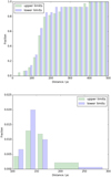 |
Fig. 6 Histograms of distances of HI features in Sco–Cen determined by association with Nai absorption lines. Top panel: cumulative histogram for all available stars. Bottom panel: histogram from stars at distances between 100 and 300 pc. More lower (upper) limits are found up to (above) about 150 pc; almost no lower limits are found above 220 pc. |
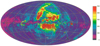 |
Fig. 7 3/4 keV map from the ROSAT all sky survey (Snowden et al. 1997). Prominent emission is seen at 300° < l < 360°, 0 < b < 30°, spatially coincident with the major part of the Sco–Cen region. The emission below the Galactic plane might be related. |
2.4 Ejecta from massive stars
Stellar winds and supernova explosions return stellar material back into the surrounding ISM. Such ejecta are enriched with products of nuclear reactions, that is, with new nuclei that were not part of the composition of gas that formed those stars. Among those new nuclei are radioactive nuclei, whose decay provides a direct observational signature of massive star feedback. The 26Al isotope witha radioactive lifetime of 1.04 Myr and emission at 1809 keV has been observed and taken as proof of current-generation massive-star nucleosynthesis (Mahoney et al. 1982; Diehl et al. 1995; Prantzos & Diehl 1996). Ejection of 26Al from a coeval group of stars is expected to commence after a few million years from the winds of the most-massive (Wolf–Rayet) stars, and continue from less massive stars and their core collapse supernovae until ≈ 30–40 Myr after the star-formation event (for details see the population synthesis study of Voss et al. 2009).
INTEGRAL with its gamma-ray spectrometer instrument SPI (Vedrenne et al. 2003) has collected significant observational data from the larger Sco–Cen region since its launch in 2002, and during the extended INTEGRAL mission. The total exposure in this region amounts to about 10 Msec, with variations of about a factor ten across the larger Sco–Cen region.
From earlier analysis of about 6 Msec of exposure after five mission years, the 26Al signal from the Sco–Cen region could be detected and discriminated from the Galaxy’s bright 26Al gamma ray emission (Diehl et al. 2010). Defining the location of 26Al-rich ejecta is the main uncertainty in such an analysis; the signal surface brightness is too faint to allow imaging from the data themselves at the required precision (see, e.g. Bouchet et al. 2015). Assuming that the Upper Sco group of stars is the most plausible source of any current radioactive 26Al from this region (cmp. Table 1), the 26Al signal was shown to be of diffuse nature and extended by about 10° in radius around (l, b) = (350°, 20°), which corresponds to about 25 pc at the distance of USco. On the other hand, if ejecta were to stream freely into the surroundings for one 26Al lifetime at typical velocities within a tenuous superbubble of ≈ 300 km s−1, the 26Al-filled region could be the entire Sco–Cen superbubble (Kretschmer et al. 2013; Krause et al. 2015, also compare the simulation below). Therefore, we may assume that these gamma-ray observations only saw a fraction of the 26Al that is located near its sources and with highest surface brightness, while the 26Al emission from more distant regions fades and becomes confused with the bright emission of the Galaxy. Still, the flux of 26Al gamma rays found with INTEGRAL in this way from USco is (6.1 ± 1.0) × 10−5 ph cm−2 s−1, and corresponds to 1.1 × 10⁻⁴ M⊙ of 26Al (Diehl et al. 2010). In a recent analysis, now from 13 yr of observations, the presence of 26Al is confirmed: for a slightly larger regionaround USco of 16° radius around (l, b) = (340°, 23°), a flux of (7.6 ± 1.4) × 10−5 ph cm−2 s−1 – corresponding to (1.3 ± 0.3) × 10−4 M⊙ of 26Al – was determined; this comprises a 6σ detection of 26Al emission from USco (Fig. 8; Siegert 2017, and in prep.). We note that the new analysis also resulted in continuum level towards Sco–Cen below the average over the sky, and therefore a negative value in Fig. 8. The 26Al measurement is relative to the continuum level and therefore not affected by this offset. Typical massive star yields of 26Al in models from Wolf–Rayet stars and core collapse supernovae are on the order of 10−5–10−4 M⊙ (e.g. Diehl et al. 2006; Chieffi & Limongi 2013), meaning that the observed 26Al is consistentwith contributions from several massive stars.
Gamma ray spectroscopy with the 26Al line has obtained a precision level that allows derivation of kinematic constraints on the radioactive ejecta (e.g. Kretschmer et al. 2013): the spectral resolution of the SPI Ge spectrometer allows one to resolve the line and determine its Doppler broadening from irregular motion of the ejecta down to ≈ 100 km s−1. Bulk velocity constraints can be derived from the line centroid, via comparison to the laboratory energy of 26Al decay (1808.73 keV; Endt 1998). An application to the signal obtained for USco indicated a bulk flow towards us at (137 ± 75) km s−1 (Diehl et al. 2010). Our re-analysis from 13 yr of INTEGRAL data confirms this, with slightly better precision, at (154 ± 53) km s−1. Any Doppler broadening of the line is constrained to below 150 km s−1 (2σ) (Siegert 2017, and in prep.).
This confirms the impression from the Hi data above (compare Fig. 5) that the sheet of dense gas that separates the local bubble from the Scorpius–Centaurus superbubble is currently eroded by the hot gas that is being pushed towards us into the local bubble.
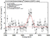 |
Fig. 8 10 Msec-INTEGRAL spectrum towards Scorpius–Centaurus in energy bands covering the 1809 keV radioactive decay line of 26A1. The signal corresponds to a 6σ detection, and is consistent with the nucleosynthesis yields of several massive stars. |
2.5 Hydrodynamic simulations of the superbubble
We used the3D mesh-refining hydrodynamics code RAMSES (Teyssier 2002) to simulate the Sco–Cen superbubble. We first performed aglobal simulation of the superbubble and then studied the reaction of a molecular cloud to the sudden pressure increase when it is overrun by a superbubble. We used a standard cooling–heating function taking into account atomic and molecular transitions. Massive star feedback is simulated by a spherical source region of 1 pc radius with mass, energy, and 26Al input rates as determined from stellar models (Fierlinger et al. 2016).
2.5.1 Global simulation
We run the global simulations in a smooth background medium. As sources we used a plausible configuration of massive stars (Table 2) given the observed stellar population (Table 1). Due to stochasticity of the IMF, the number of past supernovae is highly uncertain. To be conservative, we decided for a number of massive stars on the low side of the literature estimates (compare Table 1). The initial density distribution was homogeneous at 8.5 × 10⁻²⁴ g cm−3, consistent with the total Hi mass we find in the USco loop (104 M⊙; Gaczkowski et al. 2017) and in the wider region of 368 000 M⊙ (Pöppel et al. 2010). The initial equilibrium temperature was 1647 K and the box size  . Here, we do not attempt to include dense gas clouds. This simulation can therefore not address nested shells or details of late star formation directly. Current observations should be compared to the final state of the simulation at t = 15.8 Myr.
We show the time evolution of the simulation up to the present epoch in Fig. 9. UCL and LCC form separate superbubbles here that merge from about 5 Myr after initialisation of the simulation (10 Myr ago). The pressure during this period is consistently high, in excess of ten times that of the ambient gas.
Around 10 Myr, the superbubble again experiences high pressure due to three supernovae in LCC and UCL within about 0.1 Myr. This is of course an arbitrary feature of our modelling, but demonstrates that such a coincidence is easily possible. At this time, the superbubble has engulfed the position of USco. Any dense clouds in this region would therefore be compressed. It is possible that USco stars formed in this way. In our simulation, feedback from USco starts at this time (Fig. 9, second row).
Pressure in the superbubble then declines until the 60 M⊙ star in USco explodes (Fig. 9, third row). The superbubble again experiences overpressures in excess of a factor of ten. Any remaining clouds, possibly swept up by the wind of the 60 M⊙ star, would again be compressed and potentially prompted to form stars. This would be consistent with the recent and approximately coeval onset of star formation in the ρ Ophiuchus and Lupus I molecular clouds.
We end the simulation 1 Myr after the supernova in USco (Fig. 9, bottom row). The superbubble has now a diameter of more than 200 pc, very consistent with observations. Its shape still bears a memory of its formation history, as is the case for the real, elongated Sco–Cen superbubble.
We predict the current superbubble temperature to be spatially variable between 106 and 108 K, well inside the regime accessible by X-ray observations. This is consistent with the ROSAT detection.
The snapshots in Fig. 9 show phases of particularly high 26Al abundance. This varies by orders of magnitude during the evolution of the superbubble. During times of actively blowing massive star winds, 26Al can be restricted to less than half of the superbubble volume. For the present time, 1 Myr after the last massive star (> 15M⊙) explosion, we predict a uniform 26Al distribution. This is consistent with the updated, now more extended 26Al detection presented in Sect. 2.4.
Stars used in the the 3D hydrodynamic simulation.
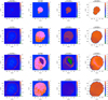 |
Fig. 9 Time evolution of the 3D hydrodynamics simulation of the Sco–Cen superbubble in a homogeneous environment. Columns from left to right: sight line-averaged logarithmic gas density, logarithmic temperature in the midplane, pressure in the midplane, and current, sight line-averaged mass density in 26Al, all in cgs units. UCL is initiated at time = 0 in the centre of the computational domain. LCC is formed at 2 Myr outside the UCL bubble, towards its lower left. At 5 Myr, the interface between the individual bubbles is eroding (top row). USco forms inside the UCL–LCC superbubble towards the upper right at 10 Myr. The expanding wind of its 60 M⊙ star is easily identified in the pressure plot at 10.85 Myr (second row). The overall pressure in the superbubble is high at this time due to two supernovae in UCL exploding at 10.48 Myr and one in LCC at 10.61 Myr. The massive star in USco explodes at 14.86 Myr. At 14.90 Myr (third row), it pressurises the superbubble again via an 26Al-rich shockwave. At the end of the simulation (15.80 Myr, bottom row, representing the present epoch), 26Al is uniformlydistributed throughout the superbubble. The pressure is low, but the temperature is still high enough to expect X-ray emission throughout the superbubble. |
2.5.2 Surrounded and squashed cloud
In order to study the effect of a superbubble engulfing a dense cloud, we first produced a turbulent cloud in a periodic box, and then put it on a RAMSES grid next to a massive-star wind.
For the turbulent cloud setup, we followed the procedure described in Moeckel & Burkert (2015). Isothermal turbulence was driven in a 10243 periodic box using the ATHENA code (Gardiner & Stone 2005, 2008; Stone et al. 2008; Stone & Gardiner 2009). Smaller scale turbulence developed self-consistently from the larger scale driving. When the turbulence was well developed, we scaled the box to 10 pc on one side, a mean number density of 100 cm−3 (giving a total mass of ≈5700M⊙) and a temperature of 10 K. The root mean square velocity of the cloud is 18 km s−1. The cloud has time to expand initially on the RAMSES grid and loses its memory of the cubic setup to some degree before significant interaction occurs.
The cloud was imported on a 3D Cartesian RAMSES grid with 20 pc on one side resolved by 128 cells. Self-gravity and adaptive mesh refinement were not used. Boundary conditions are open so that the flow may leave the box freely. The grid was initialised with a density of 2.9 × 10⁻²⁴ g cm−3, adding up to a total mass of ≈300M⊙ for the whole box. The massive star was then positioned 8 pc away from the cloud surface on one of the symmetry axes. We used the parameters for the 60 M⊙ rotating star in the models of Ekström et al. (2012) with wind properties as in Fierlinger et al. (2016).
Snapshots of the logarithmic density distribution in the midplane of the simulation are shown in Fig. 10. The massive starwind produces a typical superbubble structure, that is, a low-density bubble with a cool and dense shell that clumps due to the Vishniac instability. The superbubble starts to interact with the turbulent cloud about 0.14 Myr after the start of the simulation. Subsequently, the hot gas penetrates the low-density parts of the cloud, and surrounds the higher density parts. From 0.43 to 0.57 Myr, individual low-density regions within the cloud grow at the expense of the denser parts. Until 0.88 Myr, the cloud is completely compressed into a large number of resolution-scale fragments. While all parts of the clouds show significant motion at the start of the interaction, they have slowed down to the velocity of the hot bubble gas (0 in the frame of the simulation) towards the end by interaction with the hot gas. The typical mass of the fragments is a fraction of a solar mass. The total mass in the box at the end of the simulation is 2353 M⊙, which is almost entirely in the cold fragments.
If the fragments in our simulation represented the formation sites of individual stars, the mechanism would coordinate star formation in a volume of 10–20 pc diameter within about 0.5 Myr, much faster than the sound travel time in molecular gas for this length scale, which would be >10 Myr. This is similar to the length and timescales deduced from observations of the stars in the Sco–Cen subgroups (compare Preibisch & Mamajek 2008).
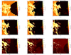 |
Fig. 10 Time evolution of a 3D hydrodynamics simulation of a turbulent cloud overrun by a superbubble. Shown are midplane slices of the density with a logarithmic colour scale at different times, as indicated in the individual panels. The dense cloud first expands due to its inherited turbulence. The shock and supershell have little impact on the dense regions of the clouds. The hot gas, however, penetrates the low-density parts of the cloud, thus surrounding the denser parts. The intermediate-density regions are therefore pushed into the dense clumps by the overpressure of the hot gas. About 40% of the initial cloud mass is squashed into distributed dense clumps in this way, after about 0.5 Myr. The rest has been swept away. A movie is provided online. |
3 Discussion: deciphering the ISM in Sco–Cen
Preibisch & Mamajek (2008) present the case for triggered star formation in USco: with a stellar velocity dispersion of ≈ 1.3 km s−1, an initial size of the stellar subgroup of 25 pc and an age spread for the stars of 1–2 Myr, the formation of the stars cannot possibly have been coordinated by internal processes in the parent cloud. An external agent associated with a characteristic velocity of at least 20 km s−1 is required. The timescale is consistent with a shockwave driven by massive star feedback in UCL that induced collapse in an existing molecular cloud.
One problem with this scenario is that any molecular clouds in the region could have also formed stars without a shockwave passing. It would therefore be unclear why star formation was not proceeding independently in such clouds for several million years. Furthermore, if the clouds were indeed present for several million years, why did the shock wave that triggered star formation in USco not trigger star formation in Lupus I, about half way to USco?
Clues might come from the results shown here, summarised in the sketch in Fig 11: in a linearly extended stream of gas, as suggested by the morphology and arrangement of the stars in Sco–Cen OB2, as well as a sequence of progressively older star clusters (Bouy & Alves 2015), superbubbles produced by massive stars will more easily break out towards the short axis of the parent cloud, similar to larger superbubbles leaving the disc of the Milky Way (compare Mac Low et al. 1989; Fierlinger et al. 2012). These superbubbles would then engulf some of the until-then more diffuse parts of the cloud. We suggest that we see this currently in USco. The Hi observations show a loop with constant diameter in adjacent velocity bins. It is therefore likely that this superbubble broke out of the parent cloud, now engulfing its remaining part, the ρ Ophiuchus and the Lupus I cloud.
Superbubbles are a very important element for understanding the system: the sound speed in superbubbles is high, varying between a few 100 and a few 1000 km s−1. This is seen in our simulation (Sect. 2.5), and supporting evidence is provided by the X-ray measurements in Sect. 2.3. Fast communication between remote parts of the cloud therefore becomes possible.
Supernovae increase the pressure in the system by typically a factor of ten or more, every few million years. More rarely, supernovae will occur within a short enough time interval (≲ few 105 yr, e.g. Krause et al. 2013) that the pressures add up. For dense gas where the effective index γ for a polytropic equation of state, p ∝ ργ, is close to one, cloud densities have to increase also by a factor of about ten.
Our simulation of a cloud initially extended over ≳ 10 pc when starting to interact with a superbubble confirms this hypothesis: the low-density regions of the turbulent cloud are penetrated by the hot bubble gas, and the intermediate-density regions are then pushed into the high-density clumps, meaning that a system of low dispersion and widely spread out clumps occurs that may form stars in a coordinated fashion. About 40% of the mass present in the initial setup has therefore fragmented into an ensemble of dense clumps with low velocity dispersion. If these clumps were the seeds of a stellar population, their low velocity dispersion and spatial extent would agree well with observations of the Sco–Cen subgroups, UCL, LCC, and USco, and other OB associations (compare Preibisch & Mamajek 2008, Sect. 6.1). This would solve the problem of how to coordinate the onset of star formation over a distance of more than 10 pc, where the velocity dispersion of the stars is only ≈ 1 km s−1. The simulation is of course highly idealised. We do not include self-gravity, which would in reality cause the cloud to contract even before the hydrodynamic effects have time to act. Had we, however, included gravity, we would not have been able to demonstrate that the hydrodynamic effects alone are sufficient and possibly decisive to produce such an ensemble of stars. Because of the lack of gravity and magnetic fields in the simulation, we do not attempt to constrain the mass spectrum of the clumps any further at this stage.
Both of our simulations neglect magnetic fields. Comparison of simulations of the larger scale ISM with and without magnetic fields show that the magnetic field generally does not impede superbubble expansion (de Avillez & Breitschwerdt 2004, 2005). Magnetic fields are important in dense gas, where they are expected to provide dynamical support (e.g. de Avillez & Breitschwerdt 2005; Inoue & Inutsuka 2008, 2012; Körtgen & Banerjee 2015; Valdivia et al. 2016) and can potentially suppress clumping instabilities (Vishniac 1983; Ntormousi et al. 2017). This may well set the actual size scales of the resulting clumps in our simulation that includes the cloud. We would also expect that the actual star formation sites are filamentary, like the dense regions in the simulations of Inoue & Inutsuka (2012), and like those seen in recent observations of Pokhrel et al. (2018). We focus here, however, on the connection to the larger scale, and refer to these other studies for details of the evolution onsmaller scales. While magnetic fields have in principle the potential to suppress the clumping instability in supershells, this is not required to explain the HI observations of the USco supershell, where the filamentary appearance of the shell suggests that the Vishniac instability is acting. Magnetic fields might, however, explain the absence of molecular gas in the HI shell around USco. We stress that the Vishniac instability is not crucial for our scenario. Suppression of instabilities at the shell surface of our global simulation would reduce the extent of the mixing zone, which is responsible for most of the radiative cooling in the bubble. This would therefore increase the size of the simulated bubble, such that a smaller number of massive stars would be required to reach the observed extent.
The blow-out of the HI supershell around USco suggests that Sco–Cen formed from a large sheet of dense gas, similar to the dense sheets in large-scale simulations of the ISM (e.g. de Avillez & Breitschwerdt 2004, 2005; Seifried et al. 2017). In these simulations, these dense sheets are “walls” of superbubbles several hundred parsecs in size. Seifried et al. (2017) show that molecular gas builds up in such sheets over millions of years. Dawson et al. (2015) may have observed this process at the interface of two HI supershells in the Carina arm of the Milky Way. Giant molecular clouds formed in this way are less violently formed than in typical colliding flow simulations of molecular cloud formation (e.g. Inoue & Inutsuka 2008; Körtgen & Banerjee 2015), because the pressure in the surrounding superbubbles is modulated by the actual energy production of the massive stars. This might make the clouds comparatively tenuous and delay the formation of stars (Dawson et al. 2015). A more gradual buildup of molecular clouds is also seen in more sophisticated, multi-phase colliding flow simulations (Inoue & Inutsuka 2012). Inutsuka et al. (2015) detail a scenario of magnetised molecular cloud and star formation along these lines. In general, molecular cloud formation at the interface of HI supershells is frequent (Dawson et al. 2013). Near the solar circle, molecular cloud formation is only weakly coupled to spiral arm passages (e.g. Koda et al. 2016).
How could the actively star-forming Lupus I cloud have formed in this scenario? Our analysis of multi-wavelength observations of the Lupus I molecular cloud resulted in a double peaked column density PDF which we interpreted as evidence for compression of part of the cloud, possibly by the most recent supernova shockwave having originated in USco (Gaczkowski et al. 2015). The two peaks differ by a factor of about three, and in the slightly denser, southern part of the cloud this was obviously enough to trigger star formation.
The gas that the Lupus I molecular cloud now consists of was probably the most tenuous part of the dense gas sheet out of which the OB association formed; otherwise, it would not be the last part to form stars. It is therefore likely that first the superbubble initially formed around UCL, and then a superbubble formed around USco, of which we still see the HI shell, thereby contributing to sweep up the gas. This has likely resulted in a denser, more compact cloud, comparable to the current extent of Lupus I. The supernova in USco 1 Myr ago could then have once more pressurised the superbubble. At this point parts of the Lupus I cloud were finally dense enough, and the hot gas penetrated the tenuous parts of the cloud, surrounded the denser regions and pushed the less dense ones into them, as shown in our simulation, and thus triggered the formation of stars. A similar scenario could apply to the nearby ρ Ophiuchus molecular cloud.
The natural timescale between major star-formation events for such a “surround and squash” scenario of propagating star formation would be the time from star formation in a region until the massive stars explode as supernovae, and the typical time in between supernovae. This is a few million years for the typical clusters of ≈ 103 M⊙ in the region. Bouy & Alves (2015) find a continuing sequence of five star-forming regions beyond LCC with similar individual masses (Piskunov et al. 2008). Their ages are within about 25 Myr, which yields timescales of a few million years between star-formation events, consistent with the scenario we propose. There is an increased time-span of about 30 Myr between the LCC and the preceding member in the sequence, IC 2602. This is, however, about the maximum expected time span in our triggering scenario, given by the main sequence lifetime of stars of 8–9 M⊙, the least massive ones that would still produce a supernova. The timescale is also consistent for triggering of USco by a supernova in UCL or LCC, and triggering of star formation in ρ Ophiuchus and Lupus I by a supernova in USco. We note that independent analysis traces the neutron star RX J1856.5-3754 back to the Sco–Cen region, and in particular USco (Tetzlaff et al. 2011; Mignani et al. 2013). The explosion date is inferred to be about 0.5 Myr ago, entirely consistent with the aforementioned results.
The process has similarities to the big superbubbles produced around disc galaxies by a jet from an active galactic nucleus (AGN) as studied in simulations by Gaibler et al. (2012). The radio lobe that surrounds the galaxy also squashes the entire gas in the galactic disc due to its large overpressure and enhances the star formation rate of the simulated galaxy.
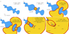 |
Fig. 11 Sketch of the evolutionary scenario on the basis of the results of the present study. Panel a: before 17 Myr ago – the elongated gas cloud in Sco–Cen has not yet formed any stars. Panel b: 17 Myr ago – something causes the onset of star formation in UCL. A superbubble forms. Panel c: 15 Myr ago – the superbubble has expanded beyond the scale height of the gas stream. It now expands quickly into more tenuous regions, but cannot penetrate into the dense clumps in the parent cloud. Panel d: 15 Myr ago – star formation starts in LCC. This could be spontaneous, or be enabled by compression by the UCL superbubble or a supernova in a more distant, older member of the elongated cloud/star cluster system. Panel e: 4–10 Myr ago – supernovae pressurise the superbubble and squash the surrounded part of the parent cloud. Star formation sets in at USco. Winds from USco then sweep up the rest of the cloud. Panel f: 1 Myr ago – a supernova in USco pressurises the superbubbleand its rim once again. Rho Ophiuchus and Lupus I begin star formation. |
4 Conclusions
We have carried out a multi-wavelength analysis of the ISM in the Sco–Cen region. From cold and tenuous to hot X-ray gas, including freshly injected nucleosynthesis ejecta, we find consistent evidence for the gradual transformation of clouds, star formation, and the expansion of the Sco–Cen superbubble. This superbubble has at times surrounded denser clouds of gas, and squashed them with the likely result of triggering more star formation. Currently, this “surround and squash” scenario predicts 26Al uniformly spread out through the cluster, which we detected with INTEGRAL. The bubble gas should have X-ray temperatures which we confirmed with X-ray images from the ROSAT all sky survey. We have performed hydrodynamic simulations that reproduce key features of our observations.
We suggest a refined scenario for the evolution of Sco–Cen: about 15–17 Myr ago star formation started in an elongated, possibly flattened gas cloud. Stars first formed in a particular part of the elongated cloud, now the UCL subgroup. A superbubble then cleared the immediate vicinity, but when it broke out, advancement of the supershell into the dense gas cloud almost stopped, and a hot bubble formed around it. Hot gas also permeated the more tenuous parts of the dense cloud inside the superbubble, but left the denser parts in place and squashed them to higher densities. This may have contributed to form the LCC subgroup. Supernovae in UCL and LCC then suddenly increased the pressure within the superbubble after several million years. This squashed some gas in the elongated cloud, now inside the superbubble, so that it collapsed gravitationally and formed stars, thus producing the USco subgroup. Massive star winds in USco then swept up the remaining parts of the cloud, leaving ρ Ophiuchus and Lupus I at opposite sides. We find kinematic and morphological evidence of shell instabilities, as might be expected for a cloud of swept-up gas. A recent supernova in USco could then have triggered star formation simultaneously in these two clouds.
This scenario of hot gas surrounding and squashing the denser parts of clouds to induce the formation of stars makes a distinctive prediction for kinematics of the new stars. The resulting star groups should be gravitationally unbound and subgroups should have coherent kinematics reflecting the local streaming velocity of the hot gas they were embedded in during the squashing. Since superbubbles can break out anisotropically from a gas distribution and have spatially and temporally varying pressure distributions (compare Fig. 9), the kinematically coherent subgroups would be expected to move in different directions, not necessarily away from the next older part in the sequence of star formation. This is similar to the observed kinematics in Sco–Cen (Wright & Mamajek 2018): the three subgroups are each unbound and have coherently moving sub-units. The velocity dispersion is so small that the groups cannot have formed on a much smaller spatial scale as bound clusters subsequently expanding due to gas expulsion.
Sco–Cen OB2 is a typical OB association. Molecular cloud and star formation appear to occur frequently in dense sheets between superbubbles (e.g. Dawson et al. 2013, 2015; Inutsuka et al. 2015; Seifried et al. 2017). A similar surround and squash mechanism might therefore operate frequently in the Milky Way and other star-forming galaxies. The surround and squash scenario might even apply to AGN-related superbubbles affecting star formation on a galaxy scale.
Movie
A movie associated to Fig. 10 Access Supplementary Material
Acknowledgements
This work was supported by funding from Deutsche Forschungsgemeinschaft under DFG project number PR 569/10-1 in the context of the Priority Program 1573 “Physics of the Interstellar Medium”. Additional support came from funds from the Munich Cluster of Excellence “Origin and Structure of the Universe” (www.universe-cluster.de). M.K. thanks the Australian Research Council for support via an Early Career Fellowship, DE130101399. We thank the anonymous referee for very useful comments that helped to improve the presentation of these results. This project has also received funding from the European Union’s Horizon 2020 research and innovation programme under the Marie Sklodowska-Curie grant agreement No 664931.
References
- Bouchet, L., Jourdain, E., & Roques, J.-P. 2015, ApJ, 801, 142 [NASA ADS] [CrossRef] [Google Scholar]
- Bouy, H., & Alves, J. 2015, A&A, 584, A26 [NASA ADS] [CrossRef] [EDP Sciences] [Google Scholar]
- Chieffi, A., & Limongi, M. 2013, ApJ, 764, 21 [NASA ADS] [CrossRef] [Google Scholar]
- Dawson, J. R., McClure-Griffiths, N. M., Wong, T., et al. 2013, ApJ, 763, 56 [NASA ADS] [CrossRef] [Google Scholar]
- Dawson, J. R., Ntormousi, E., Fukui, Y., Hayakawa, T., & Fierlinger, K. 2015, ApJ, 799, 64 [NASA ADS] [CrossRef] [Google Scholar]
- de Avillez, M. A., & Breitschwerdt, D. 2004, A&A, 425, 899 [NASA ADS] [CrossRef] [EDP Sciences] [Google Scholar]
- de Avillez, M. A., & Breitschwerdt, D. 2005, A&A, 436, 585 [NASA ADS] [CrossRef] [EDP Sciences] [Google Scholar]
- de Bruijne J. H. J. 1999, MNRAS, 310, 585 [NASA ADS] [CrossRef] [Google Scholar]
- de Geus E. J. 1992, A&A, 262, 258 [NASA ADS] [Google Scholar]
- de Zeeuw, P. T., Hoogerwerf, R., de Bruijne, J. H. J., Brown, A. G. A., & Blaauw, A. 1999, AJ, 117, 354 [NASA ADS] [CrossRef] [Google Scholar]
- Diehl, R., Dupraz, C., Bennett, K., et al. 1995, A&A, 298, 445 [NASA ADS] [Google Scholar]
- Diehl, R., Halloin, H., Kretschmer, K., et al. 2006, Nature, 439, 45 [NASA ADS] [CrossRef] [PubMed] [Google Scholar]
- Diehl, R., Lang, M. G., Martin, P., et al. 2010, A&A, 522, A51 [NASA ADS] [CrossRef] [EDP Sciences] [Google Scholar]
- Donaldson, J. K., Weinberger, A. J., Gagné, J., Boss, A. P., & Keiser, S. A. 2017, ApJ, 850, 11 [NASA ADS] [CrossRef] [Google Scholar]
- Ducourant, C., Teixeira, R., Krone-Martins, A., et al. 2017, A&A, 597, A90 [NASA ADS] [CrossRef] [EDP Sciences] [Google Scholar]
- Ekström, S., Georgy, C., Eggenberger, P., et al. 2012, A&A, 537, A146 [NASA ADS] [CrossRef] [EDP Sciences] [Google Scholar]
- Endt, P. M. 1998, Nucl. Phys. A, 633, 1 [NASA ADS] [CrossRef] [Google Scholar]
- Fierlinger, K. M., Burkert, A., Diehl, R., et al. 2012, in Advances in Computational Astrophysics: Methods, Tools, and Outcome, eds. R. Capuzzo Dolcetta, M. Limongei, A. Tomambe, & G. Giobbi, ASP Conf. Ser., 453 [Google Scholar]
- Fierlinger, K. M., Burkert, A., Ntormousi, E., et al. 2016, MNRAS, 456, 710 [NASA ADS] [CrossRef] [Google Scholar]
- Gaczkowski, B. 2016, Ph.D. Thesis, Ludwig-Maximilians-Universität, München [Google Scholar]
- Gaczkowski, B., Preibisch, T., Stanke, T., et al. 2015, A&A, 584, A36 [NASA ADS] [CrossRef] [EDP Sciences] [Google Scholar]
- Gaczkowski, B., Roccatagliata, V., Flaischlen, S., et al. 2017, A&A, 608, A102 [NASA ADS] [CrossRef] [EDP Sciences] [Google Scholar]
- Gaia Collaboration (Brown, A. G. A., et al.) 2016, A&A, 595, A2 [NASA ADS] [CrossRef] [EDP Sciences] [Google Scholar]
- Gaibler, V., Khochfar, S., Krause, M., & Silk, J. 2012, MNRAS, 425, 438 [NASA ADS] [CrossRef] [Google Scholar]
- Gardiner, T. A., & Stone, J. M. 2005, J. Comput. Phys., 205, 509 [Google Scholar]
- Gardiner, T. A., & Stone, J. M. 2008, J. Comput. Phys., 227, 4123 [NASA ADS] [CrossRef] [Google Scholar]
- Gómez, G. C., & Vázquez-Semadeni, E. 2014, ApJ, 791, 124 [NASA ADS] [CrossRef] [Google Scholar]
- Gong, M., & Ostriker, E. C. 2015, ApJ, 806, 31 [NASA ADS] [CrossRef] [Google Scholar]
- Heitsch, F., Hartmann, L. W., Slyz, A. D., Devriendt, J. E. G., & Burkert, A. 2008, ApJ, 674, 316 [NASA ADS] [CrossRef] [Google Scholar]
- Hennebelle, P., Banerjee, R., Vázquez-Semadeni, E., Klessen, R. S., & Audit, E. 2008, A&A, 486, L43 [NASA ADS] [CrossRef] [EDP Sciences] [Google Scholar]
- Herczeg, G. J., & Hillenbrand, L. A. 2015, ApJ, 808, 23 [Google Scholar]
- Inoue, T., & Inutsuka, S.-i. 2008, ApJ, 687, 303 [NASA ADS] [CrossRef] [Google Scholar]
- Inoue, T., & Inutsuka, S.-i. 2012, ApJ, 759, 35 [NASA ADS] [CrossRef] [Google Scholar]
- Inutsuka, S.-i., Inoue, T., Iwasaki, K., & Hosokawa, T. 2015, A&A, 580, A49 [NASA ADS] [CrossRef] [EDP Sciences] [Google Scholar]
- Kalberla, P. M. W., & Haud, U. 2015, A&A, 578, A78 [NASA ADS] [CrossRef] [EDP Sciences] [Google Scholar]
- Kalberla, P. M. W., McClure-Griffiths, N. M., Pisano, D. J., et al. 2010, A&A, 521, A17 [NASA ADS] [CrossRef] [EDP Sciences] [Google Scholar]
- Klose, S. 1986, Ap&SS, 128, 135 [NASA ADS] [CrossRef] [Google Scholar]
- Koda, J., Scoville, N., & Heyer, M. 2016, ApJ, 823, 76 [NASA ADS] [CrossRef] [Google Scholar]
- Körtgen, B., & Banerjee, R. 2015, MNRAS, 451, 3340 [NASA ADS] [CrossRef] [Google Scholar]
- Krause, M. G. H., & Diehl, R. 2014, ApJ, 794, L21 [NASA ADS] [CrossRef] [Google Scholar]
- Krause, M., Fierlinger, K., Diehl, R., et al. 2013, A&A, 550, A49 [NASA ADS] [CrossRef] [EDP Sciences] [Google Scholar]
- Krause, M., Diehl, R., Böhringer, H., Freyberg, M., & Lubos, D. 2014, A&A, 566, A94 [NASA ADS] [CrossRef] [EDP Sciences] [Google Scholar]
- Krause, M. G. H., Diehl, R., Bagetakos, Y., et al. 2015, A&A, 578, A113 [NASA ADS] [CrossRef] [EDP Sciences] [Google Scholar]
- Kretschmer, K., Diehl, R., Krause, M., et al. 2013, A&A, 559, A99 [NASA ADS] [CrossRef] [EDP Sciences] [Google Scholar]
- Kwon, J., Tamura, M., Hough, J. H., et al. 2015, ApJS, 220, 17 [NASA ADS] [CrossRef] [Google Scholar]
- Lindegren, L., Lammers, U., Bastian, U., et al. 2016, A&A, 595, A4 [NASA ADS] [CrossRef] [EDP Sciences] [Google Scholar]
- Mac Low, M.-M., McCray, R., & Norman, M. L. 1989, ApJ, 337, 141 [NASA ADS] [CrossRef] [Google Scholar]
- Mahoney, W. A., Ling, J. C., Jacobson, A. S., & Lingenfelter, R. E. 1982, ApJ, 262, 742 [NASA ADS] [CrossRef] [Google Scholar]
- Mamajek, E. E., Meyer, M. R., & Liebert, J. 2002, AJ, 124, 1670 [NASA ADS] [CrossRef] [Google Scholar]
- McClure-Griffiths, N. M., Pisano, D. J., Calabretta, M. R., et al. 2009, ApJS, 181, 398 [NASA ADS] [CrossRef] [Google Scholar]
- McKee, C. F.,& Ostriker, J. P. 1977, ApJ, 218, 148 [NASA ADS] [CrossRef] [Google Scholar]
- Mel’Nik, A. M., & Dambis, A. K. 2009, MNRAS, 400, 518 [NASA ADS] [CrossRef] [Google Scholar]
- Micic, M., Glover, S. C. O., Banerjee, R., & Klessen, R. S. 2013, MNRAS, 432, 626 [NASA ADS] [CrossRef] [Google Scholar]
- Mignani, R. P., Vande Putte, D., Cropper, M., et al. 2013, MNRAS, 429, 3517 [NASA ADS] [CrossRef] [Google Scholar]
- Moeckel, N., & Burkert, A. 2015, ApJ, 807, 67 [NASA ADS] [CrossRef] [Google Scholar]
- Narayan, C. A., & Jog, C. J. 2002, A&A, 394, 89 [NASA ADS] [CrossRef] [EDP Sciences] [Google Scholar]
- Ntormousi, E., Dawson, J. R., Hennebelle, P., & Fierlinger, K. 2017, A&A, 599, A94 [NASA ADS] [CrossRef] [EDP Sciences] [Google Scholar]
- Pecaut, M. J., & Mamajek, E. E. 2016, MNRAS, 461, 794 [NASA ADS] [CrossRef] [Google Scholar]
- Piskunov, A. E., Schilbach, E., Kharchenko, N. V., Röser, S., & Scholz, R.-D. 2008, A&A, 477, 165 [NASA ADS] [CrossRef] [EDP Sciences] [Google Scholar]
- Pokhrel, R., Myers, P. C., Dunham, M. M., et al. 2018, ApJ, 853, 5 [NASA ADS] [CrossRef] [Google Scholar]
- Pöppel, W. G. L., Bajaja, E., Arnal, E. M., & Morras, R. 2010, A&A, 512, A83 [NASA ADS] [CrossRef] [EDP Sciences] [Google Scholar]
- Prantzos, N., & Diehl, R. 1996, Phys. Rep., 267, 1 [NASA ADS] [CrossRef] [Google Scholar]
- Preibisch, T. 2012, Res. Astron. Astrophy., 12, 1 [Google Scholar]
- Preibisch, T., & Mamajek, E. 2008, in Handbook of Star Forming Regions: The Southern Sky, ed. B. Reipurth (San Francisco, CA: Astronomical Society of the Pacific), 235 [Google Scholar]
- Preibisch, T., & Zinnecker, H. 2007, in Triggered Star Formation in a Turbulent ISM, eds. B. G. Elmegreen, & J. Palous, IAU Symp., 237, 270 [NASA ADS] [Google Scholar]
- Preibisch, T., Brown, A. G. A., Bridges, T., Guenther, E., & Zinnecker, H. 2002, AJ, 124, 404 [NASA ADS] [CrossRef] [Google Scholar]
- Seifried, D., Walch, S., Girichidis, P., et al. 2017, MNRAS, 472, 4797 [NASA ADS] [CrossRef] [Google Scholar]
- Siegert, T. 2017, Dissertation, Technische Universität München, München https://mediatum.ub.tum.de/node?id=1340342 [Google Scholar]
- Snowden, S. L., Egger, R., Freyberg, M. J., et al. 1997, ApJ, 485, 125 [NASA ADS] [CrossRef] [Google Scholar]
- Stone, J. M., & Gardiner, T. 2009, New Astron., 14, 139 [NASA ADS] [CrossRef] [Google Scholar]
- Stone, J. M., Gardiner, T. A., Teuben, P., Hawley, J. F., & Simon, J. B. 2008, ApJS, 178, 137 [NASA ADS] [CrossRef] [Google Scholar]
- Tetzlaff, N., Eisenbeiss, T., Neuhäuser, R., & Hohle, M. M. 2011, MNRAS, 417, 617 [NASA ADS] [CrossRef] [Google Scholar]
- Teyssier, R. 2002, A&A, 385, 337 [NASA ADS] [CrossRef] [EDP Sciences] [Google Scholar]
- Valdivia, V., Hennebelle, P., Gérin, M., & Lesaffre, P. 2016, A&A, 587, A76 [NASA ADS] [CrossRef] [EDP Sciences] [Google Scholar]
- Vedrenne, G., Roques, J.-P., Schönfelder, V., et al. 2003, A&A, 411, L63 [NASA ADS] [CrossRef] [EDP Sciences] [Google Scholar]
- Vishniac, E. T. 1983, ApJ, 274, 152 [NASA ADS] [CrossRef] [Google Scholar]
- Vishniac, E. T., & Ryu, D. 1989, ApJ, 337, 917 [NASA ADS] [CrossRef] [Google Scholar]
- Voss, R., Diehl, R., Hartmann, D. H., et al. 2009, A&A, 504, 531 [NASA ADS] [CrossRef] [EDP Sciences] [Google Scholar]
- Welsh, B. Y., Lallement, R., Vergely, J.-L., & Raimond, S. 2010, A&A, 510, A54 [NASA ADS] [CrossRef] [EDP Sciences] [Google Scholar]
- Whitworth, A. P., Bhattal, A. S., Chapman, S. J., Disney, M. J., & Turner, J. A. 1994, MNRAS, 268, 291 [NASA ADS] [CrossRef] [Google Scholar]
- Wilking, B. A., Lebofsky, M. J., Kemp, J. C., & Rieke, G. H. 1979, AJ, 84, 199 [NASA ADS] [CrossRef] [Google Scholar]
- Wilking, B. A., Vrba, F. J., & Sullivan, T. 2015, ApJ, 815, 2 [NASA ADS] [CrossRef] [Google Scholar]
- Wright, N. J.,& Mamajek, E. E. 2018, MNRAS, 476, 381 [NASA ADS] [CrossRef] [Google Scholar]
This study included a much higher number of sight lines, but due to data loss the velocity values of the peaks were not available (B.Y. Welsh, 2014, priv. comm.)
The data were downloaded using the Gaia web archive: https://gea.esac.esa.int/archive/
All Tables
All Figures
|
Fig. 1 Summary sketch of observational information on the Scorpius–Centaurus region. The OB-association Sco–Cen OB2 has three subgroups of ≈2000 M⊙ each, formed over the last ≈15–20 Myr. Stars are currently forming in the ρ Ophiuchus (moving away from USco at about 1 km s−1) and Lupus I (part of an expanding Hi loop around USco) molecular clouds. See Table 1 for more details on the stars. Hi shells are detected around the youngest OB subgroup, USco, and around the entire region. Diffuse soft X-ray emission is detected towards the superbubble at a level of 1035 erg s−1. One of the detected signatures of massive star winds and supernova explosions is 26Al, towards USco. |
| In the text | |
|
Fig. 2 Planck 850 μm dust map of the Scorpius–Centaurus region in Galactic coordinates. The Milky Way plane can be seen as a pink band over the entire image. Scorpius–Centaurus OB2 (green ellipses indicate the location of the three subgroups) is mainly above the plane and is essentially dust-free apart from the ρ Ophiuchus and Lupus I clouds (labelled). Coordinates are Galactic and given in degrees. The colour scale ranges from black (low), through green, pink, red, orange to yellow (high). |
| In the text | |
|
Fig. 3 Lupus I molecular cloud: combined image of the mosaics obtained with Spitzer/MIPS at 24 μm (blue), Herschel/PACS at 160 μm (green), and the Herschel/SPIRE at 500 μm (red), all in logarithmic scales. The right overplotted panels show the column density distribution functions of the northern (top panels) and southern (bottom panels) parts of Lupus I and the central panel shows the histograms of the dust temperature in different parts of the cloud (see details in Gaczkowski et al. 2015). Left panel: gas velocity profiles averaged along cuts A, B, and C, which are highlighted by the black boxes. Ecliptic coordinates are used for this figure to help identify northern and southern parts. Galactic coordinates of the centre of Lupus I: l = 338° 50′, b = 16° 40′. |
| In the text | |
|
Fig. 4 Intensity of the 21 cm line of neutral hydrogen towards Sco–Cen. Left (right) panel: emission integrated between −20 and 0 km s−1 (0 and 10 km s−1). The numbers in the yellow boxes show upper distance limits for the Hi features derived from velocity-matched Nai absorption lines against stars with distances known from parallax measurements by Hipparcos and Gaia. |
| In the text | |
|
Fig. 5 Intensity of the 21 cm line of neutral hydrogen towards USco in the 7.4 km s−1 velocity channel (left panel) and by-eye characterisation of the Hi structures across multiple velocity channels (right panel). Three groups of rings are apparent: the USco loop (black), which corresponds to the dominant loop in the channel map on theleft, and two smaller, tube-like structures (green and red) which are cospatial but separated in velocity space. The red and green rings might be a result of erosion of the Hi interface between the Sco–Cen superbubble and the local bubble, where the hot gas streaming through the hole ablates and accelerates the Hi. |
| In the text | |
|
Fig. 6 Histograms of distances of HI features in Sco–Cen determined by association with Nai absorption lines. Top panel: cumulative histogram for all available stars. Bottom panel: histogram from stars at distances between 100 and 300 pc. More lower (upper) limits are found up to (above) about 150 pc; almost no lower limits are found above 220 pc. |
| In the text | |
|
Fig. 7 3/4 keV map from the ROSAT all sky survey (Snowden et al. 1997). Prominent emission is seen at 300° < l < 360°, 0 < b < 30°, spatially coincident with the major part of the Sco–Cen region. The emission below the Galactic plane might be related. |
| In the text | |
|
Fig. 8 10 Msec-INTEGRAL spectrum towards Scorpius–Centaurus in energy bands covering the 1809 keV radioactive decay line of 26A1. The signal corresponds to a 6σ detection, and is consistent with the nucleosynthesis yields of several massive stars. |
| In the text | |
|
Fig. 9 Time evolution of the 3D hydrodynamics simulation of the Sco–Cen superbubble in a homogeneous environment. Columns from left to right: sight line-averaged logarithmic gas density, logarithmic temperature in the midplane, pressure in the midplane, and current, sight line-averaged mass density in 26Al, all in cgs units. UCL is initiated at time = 0 in the centre of the computational domain. LCC is formed at 2 Myr outside the UCL bubble, towards its lower left. At 5 Myr, the interface between the individual bubbles is eroding (top row). USco forms inside the UCL–LCC superbubble towards the upper right at 10 Myr. The expanding wind of its 60 M⊙ star is easily identified in the pressure plot at 10.85 Myr (second row). The overall pressure in the superbubble is high at this time due to two supernovae in UCL exploding at 10.48 Myr and one in LCC at 10.61 Myr. The massive star in USco explodes at 14.86 Myr. At 14.90 Myr (third row), it pressurises the superbubble again via an 26Al-rich shockwave. At the end of the simulation (15.80 Myr, bottom row, representing the present epoch), 26Al is uniformlydistributed throughout the superbubble. The pressure is low, but the temperature is still high enough to expect X-ray emission throughout the superbubble. |
| In the text | |
|
Fig. 10 Time evolution of a 3D hydrodynamics simulation of a turbulent cloud overrun by a superbubble. Shown are midplane slices of the density with a logarithmic colour scale at different times, as indicated in the individual panels. The dense cloud first expands due to its inherited turbulence. The shock and supershell have little impact on the dense regions of the clouds. The hot gas, however, penetrates the low-density parts of the cloud, thus surrounding the denser parts. The intermediate-density regions are therefore pushed into the dense clumps by the overpressure of the hot gas. About 40% of the initial cloud mass is squashed into distributed dense clumps in this way, after about 0.5 Myr. The rest has been swept away. A movie is provided online. |
| In the text | |
|
Fig. 11 Sketch of the evolutionary scenario on the basis of the results of the present study. Panel a: before 17 Myr ago – the elongated gas cloud in Sco–Cen has not yet formed any stars. Panel b: 17 Myr ago – something causes the onset of star formation in UCL. A superbubble forms. Panel c: 15 Myr ago – the superbubble has expanded beyond the scale height of the gas stream. It now expands quickly into more tenuous regions, but cannot penetrate into the dense clumps in the parent cloud. Panel d: 15 Myr ago – star formation starts in LCC. This could be spontaneous, or be enabled by compression by the UCL superbubble or a supernova in a more distant, older member of the elongated cloud/star cluster system. Panel e: 4–10 Myr ago – supernovae pressurise the superbubble and squash the surrounded part of the parent cloud. Star formation sets in at USco. Winds from USco then sweep up the rest of the cloud. Panel f: 1 Myr ago – a supernova in USco pressurises the superbubbleand its rim once again. Rho Ophiuchus and Lupus I begin star formation. |
| In the text | |
Current usage metrics show cumulative count of Article Views (full-text article views including HTML views, PDF and ePub downloads, according to the available data) and Abstracts Views on Vision4Press platform.
Data correspond to usage on the plateform after 2015. The current usage metrics is available 48-96 hours after online publication and is updated daily on week days.
Initial download of the metrics may take a while.