| Issue |
A&A
Volume 618, October 2018
|
|
|---|---|---|
| Article Number | A121 | |
| Number of page(s) | 19 | |
| Section | Extragalactic astronomy | |
| DOI | https://doi.org/10.1051/0004-6361/201832573 | |
| Published online | 23 October 2018 | |
A mass-velocity anisotropy relation in galactic stellar disks⋆
Centro de Astronomía (CITEVA), Universidad de Antofagasta, Avenida Angamos 601, Antofagasta, Chile
e-mail: This email address is being protected from spambots. You need JavaScript enabled to view it.
, This email address is being protected from spambots. You need JavaScript enabled to view it.
Received:
2
January
2018
Accepted:
18
July
2018
Abstract
The ellipsoid of stellar random motions is a fundamental ingredient of galaxy dynamics. Yet it has long been difficult to constrain this component in disks others than the Milky Way. This article presents the modeling of the azimuthal-to-radial axis ratio of the velocity ellipsoid of galactic disks from stellar dispersion maps using integral field spectroscopy data of the CALIFA survey. The measured azimuthal anisotropy is shown to be not strongly dependent on the assumed vertical-to-radial dispersion ratio of the ellipsoid. The anisotropy distribution shows a large diversity in the orbital structure of disk galaxies from tangential to radial stellar orbits. Globally, the orbits are isotropic in inner disk regions and become more radial as a function of radius, although this picture tends to depend on galaxy morphology and luminosity. The Milky Way orbital anisotropy profile measured from the Second Gaia Data Release is consistent with those of CALIFA galaxies. A new correlation is evidenced, linking the absolute magnitude or stellar mass of the disks to the azimuthal anisotropy. More luminous disks have more radial orbits and less luminous disks have isotropic and somewhat tangential orbits. This correlation is consistent with the picture in galaxy evolution in which orbits become more radial as the mass grows and is redistributed as a function of time. With the help of circular velocity curves, it is also shown that the epicycle theory fails to reproduce the diversity of the azimuthal anisotropy of stellar random motions, as it predicts only nearly radial orbits in the presence of flat curves. The origin of this conflict is yet to be identified. It also questions the validity of the vertical-to-radial axis ratio of the velocity ellipsoid derived by many studies in the framework of the epicyclic approximation.
Key words: galaxies: kinematics and dynamics / galaxies: fundamental parameters / galaxies: stellar content / galaxies: individual: Milky Way
Full Table 1 is only available at the CDS via anonymous ftp to cdsarc.u-strasbg.fr (130.79.128.5) or via http://cdsarc.u-strasbg.fr/viz-bin/qcat?J/A+A/618/A121
© ESO 2018
1. Introduction
The random motion of stars is one of the most fundamental ingredients in the study of the dynamics of galactic disks. Among many examples showing the importance of stellar velocity dispersion in dynamics, there is asymmetric drift caused by density and dispersion gradients; this drift makes the rotation of stars lagging circular velocity. There is also the azimuthal anisotropy, which informs the structure of stellar orbits in the disk plane. Both of these make use of the azimuthal and radial components, σϕ and σR (e.g. Binney & Tremaine 2008). As for the vertical component, σz, it is essential to constrain the total mass surface density inside disks, thus the stellar mass-to-light ratios and luminous-to-dark matter fractions (e.g. Bershady et al. 2011; Martinsson et al. 2013).
It has long been a hard task to characterize the 3D velocity dispersion space of stellar disks other than the Milky Way because of the nature of observations very demanding in integration time and angular coverage. The works of Gerssen et al. (1997, 2000), Shapiro et al. (2003), and Gerssen & Shapiro Griffin (2012) made significant contributions to this field. These authors were able to constrain the vertical-to-radial axis ratio of the dispersion ellipsoid in eight spiral galaxies from long-slit spectroscopy measurements aligned with the disk kinematic major and minor axes. They found  . The growing amount of data from integral field spectroscopy (IFS) now successfully replaces such long-slit experiments, covering the 2D kinematics of the disks for large samples of galaxies. The DiskMass Survey (hereafter DMS) was exactly designed to measure dispersions in 30 low inclination disks by means of IFS and constrain the stellar mass density and luminous-to-dark mass ratio (Bershady et al. 2010a,b, 2011; Westfall et al. 2011; Martinsson et al. 2013). One of the objectives of this present study is to improve the modeling of stellar velocity dispersions from IFS data for a larger galaxy sample and larger disk inclinations.
Yet, a major problem in the derivation of the 3D dispersion space comes from the difficulty in modeling the observed dispersion σlos by (1)where ϕ is the azimuthal angle in the deprojected orbit and i the disk inclination, considering a stellar velocity ellipsoid aligned with the cylindrical coordinate system in the disk plane. Because of the competition between the components that have roughly comparable amplitudes, it impossible to fit the model blindly to the observations. To overcome that issue, one can fix one of the three parameters, preferentially σz, as the radial and tangential components can be easily disentangled in that particular case by the variation of dispersion with azimuth. For example, Noordermeer et al. (2008) assumed σϕ = σz, which allowed these authors to constrain the dispersion ellipsoid of four early-type spirals, but from long-slit spectroscopy. Although this assumption makes the derivation easier, it has no physical justification, however. Another possibility is to fix the ratio between two of the components. For instance,
  can be guessed beforehand from the slope of the rotation curve, assuming that the epicyclic approximation is valid, then σR and σϕ can be deduced with the help of the equation of the asymmetric drift to finally give
  using the dispersion data (Gerssen et al. 1997, 2000; Shapiro et al. 2003; Ciardullo et al. 2004; Gerssen & Shapiro Griffin 2012; Westfall et al. 2011). An alternate assumption is to consider global links between the components. The best example that uses such approach is DMS, which assumed
  and
and  at all galactocentric radii and for every galaxy, yielding σz by deprojecting σlos (e.g. Bershady et al. 2010a,b; Martinsson et al. 2013)
In this study I propose to relax most of these strong assumptions, by considering that only  can be fixed, making it possible to fit the two plane components to the data. Although still limited in angular and spectral resolution and spatial coverage, the current large IFS surveys such as Calar Alto Legacy Integral Field Area Survey (CALIFA, Sánchez et al. 2012), Sydney-Australian-Astronomical-Observatory Galaxy Survey (SAMI, Bryant et al. 2015), or Mapping Nearby Galaxies at Apache Point Observatory (MaNGA, Bundy et al. 2015) can yield accurate enough kinematics to make direct fits of Eq. (1) to 2D dispersion maps possible. The power of IFS devices precisely lies in the ability to recover the angular variation of velocities in the sky plane. This is an improvement with respect to the early long-slit spectroscopy works of Gerssen et al. (1997) limited to two directions only. The strategy is also different from the DMS work as the proposed model fits line-of-sight dispersions, thus avoiding problems inherent to deprojections of observables when cos ϕ and sin ϕ → 0. Moreover, the strategy is technically similar to the usual fits of velocity fields in which vlos is the projection along the line of sight of model rotation velocities vϕ and noncircular radial motions vR.
Consequently, I present the first attempt to fit 2D models of Eq. (1) to a large sample of stellar disk dispersion fields with the minimum assumptions possible and independent of any considerations imposed by the epicycle theory and asymmetric drift equations. I use the stellar kinematics of 93 disk galaxies from the CALIFA survey to derive the azimuthal anisotropy, which is the most important byproduct of this analysis (Sect. 2), study the properties of azimuthal anisotropy (Sect. 3), and compare the anisotropy distribution with the absolute magnitude and stellar mass (Sect. 4) and with predictions of the epicycle theory (Sect. 5). Brief discussions, comparisons with other works, and conclusions are presented in Sects. 6 and 7. Finally, results from the modeling of mock datasets using a N-body numerical simulation of a Milky Way-mass disk are presented in Appendices A and B. These results show the ability of the proposed strategy to find realistic azimuthal anisotropies with weak impacts from systematic effects. They also show the negative impact on  when the epicyclic assumption is assumed to be valid even though it is not.
2. Derivation of anisotropic velocity dispersions from IFS data
The observations are the integral field data from the CALIFA sample (Sánchez et al. 2012; Walcher et al. 2014). That sample is representative of the general galaxy population within the SDSS r-band absolute magnitude range [− 19,− 23.1] (Walcher et al. 2014). I used the third CALIFA release (Sánchez et al. 2016) and in particular their stellar velocity dispersion maps (Falcón-Barroso et al. 2017). All galaxies but ellipticals and S0s were selected. Moreover, disks less (more, respectively) inclined than 35° (75°) were discarded to prevent us from projection effects as much as possible. These effects have little impact on the azimuthal anisotropy for the chosen inclination disk range, as shown in Appendix A from mock data based on a N-body numerical simulation, and in Sect. 3.2. The inclinations were deduced using the photometric ellipticity e given in Falcón-Barroso et al. (2017) from cos2i = ((1 − e)2 − q0 2)∕(1 − q0 2), where q0 = 0.2 is the intrinsic axis ratio of galaxies (Chap. III, Holmberg 1946). That intrinsic ratio is known to vary with morphological type (Bottinelli et al. 1983), but for simplicity I assumed this ratio to be constant. This has no consequence on the results. Then, a visual inspection was carried out to discard the most perturbed morphologies or systems, those with clear signs of merger or strong tidal features, and a couple of disks with an axis ratio that are consistent with being less inclined than 75° but exhibit a clear edge-on morphology.
The CALIFA survey performed adaptive binning of absorption line data cubes to increase the signal-to-noise ratio of spectra. As a result, the dispersions of spaxels that are part of a same adaptive cell are equivalent. Working with individual spaxels would thus lead to correlated radii when adaptive cells extend on more than one radial ring defined below. To avoid this effect, only the spaxel lying at the center of each cell was considered in the calculation of the ellipsoid. Then, following cautions given in Falcón-Barroso et al. (2017), any σlos < 40 km s − 1 were masked to avoid the instrumental bias at observed dispersion below the spectral resolution. Also, spurious dispersions were discarded to avoid divergent fits. These were identified by inspecting by eye the distribution of σlos for each galaxy. For example, five deviant centroids above 300 km s− 1 for the galaxy UGC 312 were masked because the 93 remaining centroids in this galaxy are σlos < 170 km s− 1, or values above 600 km s− 1 for NGC 7824. A radial bin or ring is then defined by a collection of at least ten spaxels and with angular size not smaller than 2″. Such an adaptive radial sampling enabled us to perform robust least-squares fits with a number of degrees of freedom at least four times the two free parameters.
For each dispersion field, nonlinear Levenberg–Marquardt least-squares axisymmetric fits of Eq. (1) were performed at fixed disk inclination and major axis position angle, by means of the MPFIT minimization package (Markwardt 2009). The fits are made with the constraint that  is given and kept fixed as a function of radius. A large range of
  was spanned to study the impact of the vertical anisotropy parameter on the results. The ratio has been chosen randomly from normal laws centered on
  = 0.1, 0.2, 0.3,…, 1.5 with a full width at half maximum of 0.1. The boundaries of 0.1 and 1.5 for
  were chosen to be consistent with the minimum and maximum values of βz that Kalinova et al. (2017) estimated for E to Sdm CALIFA galaxies. This range also contains the values found by Gerssen & Shapiro Griffin (2012) and ratio chosen by DMS (0.6; Bershady et al. 2010a) for other galaxy samples. It also contains the compilation of values given in Pinna et al. (2018). The value
  = 0.7 is the one of the thin Galactic disk component measured in the solar neighborhood (Bland-Hawthorn & Gerhard 2016). Higher values correspond to vertical dispersions more representative of stellar populations orbiting inside a thick disk, (e.g., ∼ 1 for the thick Milky Way disk; Bland-Hawthorn & Gerhard 2016).
One thousand fits were performed for each central value of  , each time choosing randomly both the observed dispersions within the uncertainties provided by Falcón-Barroso et al. (2017), a fixed value of
  around the central values, and the initial parameter guesses of σR and
  . Normal distributions were used to select the random values. In total, 15 000 fits were thus made for each galaxy. Uniform weightings were applied to the randomly selected observed dispersions.
For each central value of  , the azimuthal anisotropy
  is chosen as the median value of the fitted distributions from the Monte Carlo fitting process. Following the analysis performed in Appendix A with mock data, I adopted as final anisotropy parameter and uncertainty at a given radius the median and standard deviation of the posterior distribution made from the 15 values of
  .
.
Finally, sample cleaning was performed by discarding the galaxies with less than three radial bins to make the derivation of median anisotropies possible for a sample as large as possible (93 disks). The sample contains 88 galaxies with an anisotropy that could be interpolated at R = h∕2, 68 at R = h, 68 at R = Re, which are not necessarily the same galaxies as those at R = h, and 19 at R = 2 h. The photometric parameters are from (the galaxy effective radius Re; Falcón-Barroso et al. 2017), and in (the disk scalelength h; Méndez-Abreu et al. 2017.) Also, 46 and 78 of the 93 galaxies have measured bar and bulge properties, respectively (Méndez-Abreu et al. 2017). This information can be used to study the impact of the bulge and the bar on the anisotropy (Sect. 3.3). The working sample is made of 8 galaxies that are classified Sa, 9 Sab, 24 Sb, 35 Sbc, 8 Sc, 5 Scd, 2 Sd, 1 Sdm, and one Irr within the absolute magnitude range [− 19.2,− 22.8]. The sample is thus neither uniform nor complete and the lack of objects at the faint magnitude end reflects the difficulty of measuring absorption lines in later disk morphologies.
It is important to note that the stellar or gaseous rotation curves of these galaxies have not been derived. The velocity curves used to test the epicyclic approximation are those given by Kalinova et al. (2017) for the CALIFA sample, and by Epinat et al. (2008a,b) for another galaxy sample (see Sect. 5).
Also, for sake of comparison I derived the azimuthal anisotropy profile of the Milky Way. For that, I used astrometric and spectroscopic data of the Gaia mission (Gaia Collaboration 2016), and particularly the radial and azimuthal dispersions performed by D. Katz (priv. comm., and see details in Gaia Collaboration 2018b). These data consist in millions of FGK stars selected in the Second Gaia Data Release (Gaia Collaboration 2018a), lying in the Galactic disk (4 ≤ R ≤ 14 kpc, |ϕ| ≤ 15°, |z| ≤ 1 kpc). Although it does not represent kinematic measurements of the entire Galaxy, and though the methodology is very different from that used to model the CALIFA dispersion fields, this large set of stars is enough to infer a robust Galactic anisotropy profile that is certainly of better quality than any of the other galaxies studied here.
3. Properties of azimuthal anisotropy
3.1. Examples of results
Figure 1 presents typical results obtained from the least-squares fits. The shown galaxy is NGC 257 (i = 51°), which is a Sc galaxy from the CALIFA subsample that has 206 useful centroid spaxels spread over 12 independent adaptive radial bins. Examples of results for 4 other galaxies are shown in Appendix C. The middle panel shows all the spaxel values by different colors, and the expected decrease of the dispersion as a function of radius. The azimuthally averaged dispersion profile is shown as open circles, and the azimuthal average from the resulting 2D dispersion model as a thick blue line, highlighting the ability of the axisymmetric model to capture the bulk of the random motions.
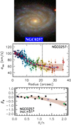 |
Fig. 1 Example of results with the galaxy NGC 257. Top: composite SDSS image of the galaxy. Middle: line-of-sight dispersion profile. A rainbow color code is used to highlight the common spaxel centroids inside the adaptive radial rings. The shaded area represents the standard deviation of σlos inside each adaptive ring. Red open circles represent the azimuthally average of σlos within each radial ring. The thick blue line indicates the azimuthally average of the dispersion model done with |

The azimuthal anisotropy profile is shown in Fig. 1 (bottom panel, filled circles). The scatter of βϕ at each radius remains small within the spanned range of  (except at R ∼ 1.45 h). This indicates that βϕ is not strongly dependent on the choice of
  in stellar disks, whose finding agrees with the results obtained from the modeling of mock data using a N-body simulation (Appendix A). This result is well representative of the whole sample. The anisotropy profile of NGC 257 is consistent with isotropy in the inner disk (βϕ ∼ 0) and then with more tangential stellar orbits in outer regions. The shaded area shows the scatter of 1000 second degree polynomial fits to random anisotropy profiles chosen within a Gaussian law of standard deviation the quoted uncertainties of the filled circles. The polynomial fits make it possible to interpolate the profile at the characteristic radii R = Re and R∕h = 0.5, 1, 2, whenever possible. Table 1 lists the interpolated anisotropies at these radii as well as the median of the profile.
Azimuthal anistropy of 93 disk galaxies from the CALIFA sample.
Figure 2 presents azimuth-dispersion diagrams at selected radii for nine galaxies. The radial ranges are 11.9″–22.6′′ (NGC 755), 13.3′′–15.4′′ (NGC 5633), 5.4′′–7.6′′ (IC1528), R = 1′′–9.4′′ (NGC 257), 5.4′′–9.4′′ (NGC 5016), 1.1′′–8.1′′ (IC 456), 7.3–13.8′′ (NGC 2253), 3.2′′–11.6′′ (NGC 4047), and 13.7′′–22.3′′ (NGC 5406). The radial range shown for NGC 257 corresponds to the isotropic orbits observed in the four innermost radial bins in Fig. 1. The solid lines are the model line-of-sight dispersion, as deduced from anisotropies averaged over the considered radial ranges. The azimuth-dispersion diagrams are evidence of many irregularities in the dispersion maps. Some diagrams seem scattered (e.g., NGC 755, NGC 5633, IC 4566), others present wiggles on small angular scales (e.g., NGC 4047, NGC 5016, NGC 5406), others show asymmetries in the amplitude of the anisotropy from one side of the galaxy to the other (e.g., ϕ = π∕2 versus ϕ = 3π∕2 for NGC 2253). These asymmetries are caused by lopsidedness, spiral arms, and bisymmetric or other higher frequency perturbations in the disks. They obviously cannot be reproduced by axisymmetric modeling.
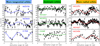 |
Fig. 2 Azimuth-velocity dispersion diagrams for 9 example galaxies. From left to right (respectively) the columns illustrate orbits that are more tangentially biased (βϕ → − 0.5), isotropic (βϕ ∼ 0), and more radially biased (βϕ → 0.5). Symbols are the CALIFA line-of-sight velocity dispersions and colored curves the best-fit anisotropic dispersion model (for the case |

3.2. Global properties
The distribution of the median anisotropy as a function of disk inclination is shown in the top panel of Fig. 3. It shows the negligible projection effect on the derived anisotropy, as the median anisotropy is consistent with being not strongly correlated with the inclination. Whether the slight trend of smaller βϕ in disks of lower inclination is genuine or an artifact from having fewer such disks in the sample is not clear. A larger sample would be helpful to clarify that point. What is clear however is the inclination effect with the median uncertainty (bottom panel). This implies that the accuracy of the modeling is lower for lower inclinations. It is important to note that this trend is in good agreement with the expectations from the analysis of the mock datasets of Appendix A (solid line in Fig. 3). It is evidence that the proposed uncertainties on observed anisotropies are realistic, and that the trends obtained from the analysis of mock low-resolution dispersion maps are representative of real observations.
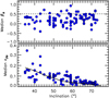 |
Fig. 3 Median anisotropy and uncertainty (ϵβϕ) as a function of disk inclination for the CALIFA disk galaxies. The horizontal dashed line is βϕ = 0.51 chosen by the DiskMass Survey (Bershady et al. 2011). The solid line is not a fit to the data but the uncertainty curve deduced from the mock data of Appendix A, showing the consistency between the observations and numerical modeling. |
The profiles of azimuthal anisotropy as a function of galactocentric radius for the 93 galaxies are shown in Fig. 4 (open circles). The galaxy distances used to transform the radius into a kpc-scale are those listed in Nasa NASA/IPAC Extragalactic Database. The median profile is also shown (filled diamonds) as well as the standard deviation on each bin of radius (dashed lines). Based on prescriptions given in Binney & Tremaine (2008), several types of orbits can be identified as follows: tangential orbits (βϕ <− 0.5), intermediate tangential-to-isotropic orbits (− 0.5 < βϕ < − 0.25), isotropic orbits (|βϕ| ≤ 0.25, with pure isotropy at βϕ = 0), intermediate isotropic-to-radial orbits (0.25 < βϕ < 0.5), and radial orbits (βϕ > 0.5). Radii with very tangential orbits βϕ ≪ − 5 that are proxies of circular orbits (βϕ → − ∞) are not observed. We note the effect of the orbits in the azimuthal-dispersion diagrams of Fig. 2. The largest values of σlos are reached at ϕ = (0,π) for more tangential orbits, ϕ = (π∕2, 3π∕2) for more radial orbits, whereas σlos is nearly flat for isotropic orbits, according to Eq. (1).
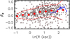 |
Fig. 4 Azimuthal anisotropy profiles for the sample of 93 CALIFA disk galaxies(circles).The filled diamonds represent the median profile derived from every galaxy and the dashed lines the standard deviation. The solid line indicates the anisotropy profile oftheMilkyWayasdeducedfromGaiaDataRelease2dispersions published in Gaia Collaboration (2018b), and an open triangle the location of the Sun. |
The median anisotropy for the sample is βϕ = 0.25 and the median profile as a function of radius is consistent with orbits that turn from isotropic at low radius to more radially biased orbits at larger radius. This radial trend also seems to depend on the morpholigical type (see Sect. 4). Another consequence of Figs. 3 and 4 is the observation that βϕ = 0.51, as assumed by the DMS analysis (Bershady et al. 2010a,b; Martinsson et al. 2013), cannot be a value representative of nearby disks of any morphological types and at every galactocentric radii.
The Gaia DR2 anisotropy profile of the Milky Way compares well with the values measured for the other galaxies (solid line in Fig. 4). It rises as a function of radius, giving a solar neighborhood value consistent with radially biased orbits (open triangle). It is important to note that the value chosen by Bershady et al. (2010a,b) and Martinsson et al. (2013) agrees perfectly with that of the solar neighborhood, as already reported in Bershady et al. (2010b).
3.3. Impact of bars and bulges
The variation of anisotropy as a function of bulge-to-total (B/T) and bar-to-total r-band luminosity fractions is shown in Fig. 5. It is useful to assess globally the impact of the stellar bulges and bars onthe median velocity anisotropy in the disk planes.
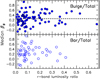 |
Fig. 5 Median anisotropy as a function of B/T (top) and bar-to-total (bottom) luminosity fraction in the SDSS r-band. A horizontal dashed line indicates the median anisotropy of the galaxies with lower bulge contribution (bulge-to-total luminosity fraction lower than 20%). |
In particular, verifications were made that the galaxies with larger bulge contributions to the total galaxy luminosity are not systematically more isotropic/anisotropic than the rest of the sample. Indeed, the relevance of performing fits of the planar model of Eq. (1) to dispersions of stars potentially more impacted by spherical or triaxial symmetries could be questioned. The verification is shown in the top panel of Fig. 5. No systematic trends are observed; the anisotropy of the galaxies with a more important bulge contribution (B∕T > 20%) remains in full agreement with the median anisotropy of the galaxies with a smaller bulge contribution (B∕T ≤ 20%, dashed line). Then, verifications were also made that no systematic trend occurs when B/T is compared to the anisotropy interpolated at the bulge effective radius R = Rb.
A similar comparison with the luminosity contribution of the bar was carried out. As the dynamics of bars participate in the secular evolution of disks, it might be possible to observe an effect on the structure of the stellar orbits as a function of bar importance. This is however not the case, as shown in the bottom panel of Fig. 5. As in the bulge case, the anisotropy distribution remains roughly constant as a function of the bar-to-total luminosity fraction. This could indicate a more important role from other mechanisms than stellar bars in shaping the global orbital structure in the plane of galactic disks.
4. Evidence for a link between azimuthal anisotropy and the magnitude and morphological type
The radial variation of βϕ can also be measured in bins of luminosity and morphological types. This is shown in Fig. 6, which reveals a link between the anisotropy and morphology (top). The earlier the type of the disk, the more radially biased the stellar orbits. Anisotropy parameters in Sa-Sab show small differences with Sb types. The radial change of anisotropy seems linked to the morphology as well. Globally, it increases with radius in Sa, Sab, and Sb types, increases slightly in Sbc-Sc disks, and tends to decrease in types later than Scd. Interestingly, the anisotropy seems roughly independent on type in the innermost regions.
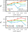 |
Fig. 6 Azimuthal dispersion profiles color-coded with the morphological type (top) and absolute r-band magnitude (bottom). |
The bottom panel of Fig. 6 also identifies a clear link with the absolute r-band magnitude (thus with the stellar mass). Unsurprisingly, the relation looks similar to the top panel, in which the median anisotropy is larger in more luminous disks.
The link with the luminosity can also be studied at characteristic radii. Figure 7 shows for instance the azimuthal anisotropy at R = h∕2 and R = h as a function of magnitude; symbol shapes and colors are coded as functions of morphological types. The anisotropy and magnitude at R = h∕2 present a non-negligible degree of correlation (Pearson correlation factor of 60%), but also non-negligible scatter.
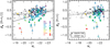 |
Fig. 7 Absolute magnitude-anisotropy relations of CALIFA stellar disks at R = h∕2 (left) and R = h (right). Different colors and symbols represent different disk morphologies from Sa to Irr. The solid line is the most likely linear fit to βϕ (at R = h∕2 only). Crossed symbols and dotted lines represent the observed and best-fit relations predicted by the epicycle approximation for the same CALIFA disks, as deduced from circular velocity curves of Kalinova et al. (2017). Gray circles and dashed lines are the observed and best-fit relations predicted by the epicycle approximation for other galaxies, as deduced from Hα rotation curves of the GHASP sample of Epinat et al. (2008a,b). |
A linear model βϕ = aMr + b has thus been fitted to the relation. This can be achieved by iterative least-squares fits coupled with sigma-clipping of the most deviant points. However a more robust solution for scattered correlations is to account for an additional intrinsic variation perpendicular to the model (e.g. Hogg et al. 2010). A linear Bayesian estimation turns out to be more appropriate in this case. It has been performed with the Python library emcee developed by Foreman-Mackey et al. (2013), which makes use of the affine-invariant ensemble sampler Goodman & Weare (2010) in the Markov chain Monte Carlo fit (MCMC). The likelihood function introducing the Gaussian variance s due to the point scattering perpendicular to the line is given in Hogg et al. (2010). The corner plot reporting the projections of the posterior probability distributions of the two parameters and of ln(s) is shown in Fig. D.1.
The linear relation the most likely is (2)where the slope, intercept, and lower and upper uncertainties are based on the 50th, 16th, and 84th percentiles of the samples in the marginalized distributions, respectively. The larger scatter of βϕ at R = h makes the correlation poorer (correlation factor of 30%) and the linear fit difficult. This correlation is mostly valid for disks brighter than with Mr = − 20 because of the lack of observations of fainter galaxies. It would therefore be important to extend this type of analysis using a more complete sample at the faint magnitude end. This could only be achieved from more accurate and sensitive observations than CALIFA. Integral field spectroscopy with, for example, the Very Large Telescope MUSE instrument (Bacon et al. 2010) would be certainly appropriate for that work. That absolute magnitude-anisotropy relation is translated into a stellar mass-anisotropy relation in Sect. 6.
5. Disagreement with the epicyclic approximation
In the framework of the epicycle theory, the azimuthal anisotropy is linked to the slope of the circular velocity vc (e.g. Binney & Tremaine 2008) by (3)
(3)
The objective of this section is to present a comparative analysis of the epicycle anisotropy βEA to the stellar azimuthal anisotropy. This goal is achieved by means of two samples of velocity curves that make it possible to derive the difference Δβϕ = βϕ − βEA and the distribution of anisotropies at characteristic radii (R∕h = 0.5, 1, 2 and R = Re).
The first set of data are the circular velocity curves of CALIFA galaxies derived by Kalinova et al. (2017). As these authors fit the mass distribution and gravitational potential to the data from dynamical modeling involving anisotropic multi-Gaussian expansion (Cappellari 2008), they were able to infer the circular velocity curves of the galaxies. I thus derived the profiles of βEA for the 68 galaxies in common with their CALIFA sample, as well as Δβϕ. An example of an epicycle anisotropy profile is shown in Fig. 1 with the galaxy NGC 257, and in Appendix C for a few other galaxies.
Moreover, the circular velocity can be reasonably approximated by the rotation curve vϕ of a gaseous component because the gas rotation does not lag vc as significantly as stars. This assumption allowed Gerssen et al. (1997, 2000), Shapiro et al. (2003), Ciardullo et al. (2004), Gerssen & Shapiro Griffin (2012), and Westfall et al. (2011) to derive  beforehand, then find σϕ, σR and σz using the line-of-sight dispersions and the equation of the asymmetric drift, to finally deduce
  . Therefore, a second set of kinematical data does not involve CALIFA, and instead uses Gassendi Hα survey of SPirals (GHASP), a high-resolution Fabry–Perot interferometry survey of Hα gas velocity fields and rotation curves of 203 nearby disk galaxies (Epinat et al. 2008a,b). The GHASP sample presents a couple of advantages. First, it has negligible overlap with CALIFA. This implies that it can be used as an independent consistency check in the analysis. Then, its angular and spectral resolution is higher than CALIFA. As the slope of vϕ is the key factor of Eq. (3), the better the resolution, the less biased the analysis of βEA. This is the reason why no attempt to derive gas rotation curves of the present CALIFA sample was performed.
The GHASP sample contains all types of disk morphology over a large range of magnitude and rotation velocity. A selection was made to keep only the GHASP targets with available Rc surface photometry from Barbosa et al. (2015). The Rc magnitudes of GHASP can be used as good proxies of the SDSS r magnitudes, with a difference between the two photometric systems within ± 0.2 magnitude only, on average (Barbosa et al. 2015). A three-parameter velocity model was fitted to the GHASP rotation curves to avoid sudden ring-to-ring change of velocity slope inherent to the high-resolution Fabry–Perot data. The model is the Einasto velocity profile presented in Chemin et al. (2011). The disk scalelengths of GHASP are given in Barbosa et al. (2015). If no scalelength is provided in Barbosa et al. (2015), then it was deduced from the galaxy effective radius by h = Re∕1.7. An example of rotation curve and epicycle anisotropy profile is shown in Fig. 8 with the galaxy UGC 3809. The selection led to a total of 128 galaxies with βEA at R = h, without objects in common with the CALIFA sample.
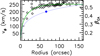 |
Fig. 8 Hα rotation curve (vϕ, open symbols and solid line) and the epicycle anisotropy profile (βEA, dotted line) of the galaxy UGC 3809. The Hα rotation curve is from the GHASP survey (Epinat et al. 2008a,b). The solid line indicates the Einasto model of the rotation velocity. The βEA profile is deduced from the rotation model using Eq. (3). The filled circles represent βEA at R = h. |
It is important to note that in the considered range of magnitude, the fraction of galaxies fainter than Mr = − 20.5 is larger in GHASP than in CALIFA, and the fraction of galaxies brighter than Mr = − 22.1 is larger in CALIFA than in GHASP. It is indeed more difficult for GHASP to detect Hα emission at high stellar mass and more difficult for CALIFA to detect absorption lines from colder (lower dispersion) stellar disks. This has no impact on the result, however.
The normalized distribution of residuals Δβϕ is shown in the top left panel of Fig. 9. This figure also presents the normalized distributions of βϕ and βEA at R∕h = 0.5, 1, 2 and R = Re (R = h for GHASP).
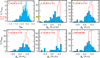 |
Fig. 9 Comparisons of stellar anisotropy βϕ and epicycle anisotropy βEA. All panels show normalized distributions in %. The bottom right panel compares the stellar anisotropy from CALIFA with the epicycle value derived from Hα rotation curves of the GHASP sample of Epinat et al. (2008a,b), while all other panels compare the stellar anisotropy from CALIFA with the epicycle value derived from CALIFA circular velocity curves of Kalinova et al. (2017). The top left graph is the total distribution of differences Δβϕ = βϕ − βEA for the 68 CALIFA galaxies with common βϕ and βEA. Blue shaded histograms are those of the stellar anisotropy, and red histograms those of the epicycle anisotropy. |
The distribution of epicycle anisotropy for the GHASP galaxies is very comparable to that of CALIFA. A difference of ∼0.1 only is observed between the two samples (GHASP values tend to be smaller). This indicates a good consistency between the two datasets of velocity curves. Ionized gas rotation curves tend to be only slightly less flat than the circular velocity curves of Kalinova et al. (2017) at the considered radius, perhaps highlighting a small asymmetric drift in the gaseous component.
More interestingly, significant discrepancies between stellar and epicycle anisotropies are evidenced. Δβϕ that are consistent with the null value within the quoted uncertainty of 0.15 represent only 1/3 of all values. The residuals are mainly negative. The concentration of epicyclic approximation around ∼ 0.3− 0.5 makes the theory overestimate the number of galaxies with intermediate isotropic-to-radial and radially biased orbits, up to a factor of 2 − 6, depending on the considered radius. The variation of Δβϕ as a function of radius for the 68 galaxies in common with Kalinova et al. (2017) is shown in Fig. 10. It is seen that, on average, larger anisotropy residuals occur at low radius, as caused by the larger occurrence of isotropic orbits in inner disk regions (Fig. 4); smaller residuals occur at larger radii, although with a significant scatter.
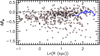 |
Fig. 10 Radial profiles of difference between the stellar anisotropy βϕ and the epicycle anisotropy βEA = Δβϕ. The solid line indicates Δβϕ for the Milky Way, as derived from Gaia DR2 data published in Gaia Collaboration (2018b). The location of the Sun is indicated by a triangle. |
I also measured the epicycle anisotropy of the Milky Way between R = 4 and R = 13 kpc using a third degree polynomial fit of the azimuthal velocity curve of stars within |z| = 200 pc of the disk measured in Gaia Collaboration (2018b) from Gaia DR2 data, as well as between R = 4 and R = 8 kpc using a Einasto model of the Hi rotation curve measured in Chemin et al. (2015). I found Galactic βEA between 0.4 and 0.6, which is thus different from the real Galactic anisotropy profile of Fig. 4 by Δβϕ = 0.1 to 0.25 inside R ∼ 7 kpc (solid line in Fig. 10). Therefore, Eq. (3) of the epicyclic approximation does not apply completely to the inner Galactic kinematics either. In the solar neighborhood, the epicycle anisotropy matches well the stellar value (triangle symbol in Fig. 10).
A direct consequence of these results is the significant possibility that the azimuthal anisotropy chosen by Gerssen et al. (1997, 2000), Shapiro et al. (2003), Ciardullo et al. (2004), Westfall et al. (2011), and Gerssen & Shapiro Griffin (2012) is inappropriate, because these authors all assumed βϕ = βEA. Since the impact of this assumption is negative on the estimation of the vertical-to-radial dispersion ratio (see Appendix B), I did not attempt to derive βz at fixed βEA.
The epicycle anisotropy is shown as a function of absolute magnitude in Fig. 7 at R = h∕2 and R = h. The two values are correlated at both radii. The epicycle relations can be modeled by the linear equations (4)at R = h/2 and
 (5)at R = h, again considering Mr ∼ MR. This parametrization is shown as dashed and dotted curves in Fig. 7. The slopes of the CALIFA and GHASP relationships are sensitively similar. The zero points are different, but that difference is not significant as it includes the systematic ∼0.1 difference between the two samples mentioned above and is within the errors.
It is important to note that if the epicycle approximation was able to produce correct anisotropies, it would automatically imply an absolute magnitude-anisotropy relation. Even though this correlation actually has different parameters, the correlation observed between stellar anisotropy and magnitude would thus be supported by theoretical expectations. In reality, the epicycle relationship is shallower than the magnitude-anisotropy relation at R = h∕2. This also suggests that the failed detection of a clear correlation at R = h may be fortuitous. A larger sample would certainly clarify that point.
6. Discussion
The advent of large IFS surveys such as CALIFA (Sánchez et al. 2012), SAMI (Bryant et al. 2015), and MaNGA (Bundy et al. 2015) is an opportunity to understand better the dynamics and evolution of stellar disks. With such data, it has been shown it is possible to measure the velocity anisotropy in the disk plane from a simple geometric and kinematic model of dispersion fields, as for velocity fields, and with minimum assumptions. This is a major improvement with respect to early slit measurements, although not enough to get strong constraints on the vertical-to-radial axis ratio of the ellipsoid. A significant range of vertical-to-radial dispersion ratio can indeed be invoked to get the value of the azimuthal anisotropy parameter (Sect. 3.2). This does not necessarily imply that a link does not exist between βϕ and βz within the sample, however.
The best way to determine unambiguously all parameters remains the observations of face-on disks (e.g., the DMS survey) and the direct measurements of vertical dispersion in a wide variety of luminosities and morphologies, and then fix σz in Eq. (1) while fitting the dispersion maps of the present CALIFA subsample. This type of analysis will be investigated in future works. It is important to note that this should work well only if clear relation(s) between σz and fundamental galaxy properties can be identified.
6.1. Relation between the stellar mass and shape of stellar orbits
Schwarzschild orbit modeling is another possible way to constrain the orbital structure of stellar triaxial systems (Schwarzschild 1979). This method was used very recently to model the whole CALIFA sample, i.e., also including ellipticals and lenticulars (Zhu et al. 2018a,b). These authors found a broad range of types of orbits inside Re at a given stellar mass, but noticed a trend in the links between the stellar mass and shape of orbits. Counter-rotating orbits represent ≲10% of the galaxy populations; warm orbits dominate the galaxy luminosity fraction at a level of 40% for M⋆ ≲ 1011 M⊙; the fraction of hot orbits increases from 2 × 10¹⁰ M⊙ and dominates at large mass, while that of colder orbits contribute to 10–30%, being more important around M⋆ = 1010 M⊙. These authors defined cold orbits by near circular orbits; warm orbits by those with substantive angular momentum, but harboring more extensive radial motions; and hot orbits by those with negligible angular momentum.
Making the comparison with their analysis is not straightforward as they measured a circularity parameter, which differs from βϕ. Moreover, the present methodology is not designed to differentiate prograde from retrograde orbits. To force the comparison with Zhu et al. (2018b), I used the stellar mass given in Falcón-Barroso et al. (2017) to recast the magnitude-anisotropy relation into a mass-anisotropy relation (Fig. 11), and measure the fractions of three broader families of orbits in the plane, i.e, tangential (βϕ < − 0.25), isotropic (|βϕ| ≤ 0.25) and radial (βϕ > 0.25) orbits, in bins of 0.5 dex of stellar mass. For each galaxy, the global anisotropy is chosen as the median value of the radial profile, and the associated error is the median of the anisotropy uncertainties. With those definitions, it is shown that the fraction of tangential orbits is unsurprisingly negligible and the fraction of isotropic orbits decreases with the stellar mass to the detriment of radial orbits, which start dominating the sample at log(M⋆∕M⊙) ∼ 10.5. Therefore, the trends measured by Zhu et al. (2018b) are qualitatively present within the three categories of orbits if a rough parallel is made between warm with isotropic orbits, hot with radial orbits and cold with tangential orbits, and with some obvious overlap between warm with radial orbits and cold with isotropic orbits. These results indicate the important role of galaxy evolution in shaping the stellar orbits in the plane. As the morphology changes with time and as the mass grows and is redistributed through various dynamical effects, the tangential and isotropic orbits in disks turn progressively radial.
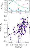 |
Fig. 11 Stellar mass-azimuthal anisotropy correlation. The top panel shows the occurrence of galaxies per bin of stellar mass with isotropic, radial and tangential orbits (circle, triangle, and squared symbols, respectively), normalized to the total number of galaxies per 0.5 dex bin of stellar mass. The mass unit is M⊙. The starred symbol is for the Milky Way. The solid line is the most likely linear model of the mass-anisotropy relation given by Eq. (6). |
The mass-anisotropy correlation of Fig. 11 can be modeled by the following linear law: (6)This model is shown as a solid line in Fig. 11. Appendix D gives posterior distributions of the MCMC fits, again performed with a nuisance parameter controlling the scatter perpendicular to the law.
During the refereeing step of this article, Pinna et al. (2018) published a detailed analysis of the impact of many dynamical processes on  from idealized and cosmological simulations. They found that the vertical-to-radial axis of the velocity ellipsoid can be produced by a multitude of disk heating mechanisms (bars, mergers, and spiral arms). They also analyzed a compilation of
  from photometry and spectroscopy-based observations and came to the conclusion that no correlation exists between the morphological type and vertical anisotropy parameter, in contrast with claims of Gerssen & Shapiro Griffin (2012). The study of a range of simulated galaxy mass larger than that of Pinna et al. (2018) would be useful to investigate whether the new magnitude and mass-anisotropy correlations shown in this work are present in cosmological numerical models as well. If present, such simulations could likely identify which of the secular and hierarchical mechanisms participates the most in the building of that relation.
Finally, the location of the Milky Way in the stellar mass-anisotropy diagram matches perfectly within the observed correlation. The mass of the Milky Way takes into account the stellar masses of the bulge, thin and superthin bars, thick and thin disks and outer halo, as given in Bland-Hawthorn & Gerhard (2016). The median value is that of the Galactic profile shown in Fig. 4.
6.2. Epicycle anisotropy versus stellar azimuthal anisotropy
The difference between the anisotropy parameters measured from stellar dispersions and predicted from the epicycle approximation can be seen as a problem of slope of rotation curves with respect to the measured anisotropies: there are too many galaxies harboring an almost flat velocity curve. This problem is manyfold.
First, the rise of the galaxy rotation curves is not steep enough to explain the occurrence of isotropic and more tangential orbits. In the context of the epicycle approximation, isotropy can only be obtained when the velocity is linearly dependent on radius. As for tangential motions, βϕ = − 0.5 can only be obtained with vc ∝ R 2, assuming a spherical distribution of total dark + luminous matter. Besides the fact that such latter velocity shape has never been observed in galaxies, it is that of a mass distribution that increases as R 4 (the density linearly increases with radius), which is not physical. In presence of almost flat velocity curves, the nominal equation of βEA thus excludes the tangential orbits for realistic mass distributions, and, by extension, the circular orbits (βϕ → − ∞). This may seem paradoxical because the epicyclic approximation is supposed to explain motions of stars very weakly perturbed, almost circular.
Then, there are not enough steeply declining rotation curves to explain the occurrence of the most radial orbits (βϕ > 0.5). It is indeed very rare to find declining curves, particularly at the radii probed here, knowing that the maximum of rotation curves are usually observed around R = 2.2 h where the amplitude of the contribution of an exponential stellar disk is maximum (Freeman 1970).
I exclude the possibility of incorrect derived anisotropies for the stellar data as origin of the discrepancy. The analysis of a numerical simulation shows that the azimuthal anisotropy inferred from fits of Eq. (1) is not strongly deviant from the simulated values. The systematic offset is ∼ 0.1 at most and occurs only at low inclination, and the typical uncertainty is 0.15 (see Appendix A). In other words, the level of inaccuracy of the proposed methodology is not enough to confuse orbits that are genuinely radial with more isotropic and tangential orbits.
It is not possible to identify the origin of the discrepancy with the current analysis. More observations of cold stellar disks are necessary to study this problem, particularly at low disk stellar mass where the difference is stronger. Similarly, other observations probing outer regions would be helpful to verify whether the problem still holds where the disks are colder and the rotation curves flatter. Moreover, numerical simulations would be helpful to assess the domain of suitability of the theory with realistic stellar orbits. That would imply studying both the simulated dynamics of low mass, unevolved disks, and that of massive, evolved disks, i.e., those which have been dynamically heated by a large diversity of disturbing mechanisms that the theory cannot address (tidal encounters, mergers, accretion of intergalactic gas, spiral arms, bars, lopsidedness, interactions between Giant Molecular Clouds, etc.). The test of Eq. (3) with the N-body simulation of a barred spiral disk in Appendices A and B is a first step toward these objectives. Additionally, Cuddeford & Binney (1994) proposed a modified version of Eq. (3), but it has never been tested with extragalactic data. This possibility shall be explored in future works.
7. Summary
In this article, I have derived the azimuthal anisotropy of velocity dispersions in the plane of stellar disks by means of a simple kinematic and geometric model fitted to dispersion maps from the IFS CALIFA survey, assuming fixed vertical-to-radial dispersion ratios. The testing of the validity of the methodology applied to a N-body numerical simulation of a Milky Way-like disk gave full satisfaction. It showed the negligible impact of systematic inclination, angular resolution, and noise effects, which do not prevent the algorithm from finding different families of simulated stellar orbits.
The main conclusions from this work are as follows:
-
Stellar disks exhibit a broad variety of tangential, isotropic, and radial orbits, yet isotropic to radially biased orbits are more frequent.
-
Globally, stellar orbits in the plane tend to be more and more radial with radius. This figure nonetheless depends on the morphology and absolute magnitude of the galaxies.
-
Evidence for an absolute magnitude-, or stellar mass-, azimuthal anisotropy correlation is presented. Disks with lower stellar mass exhibit more tangential and isotropic orbits, while more massive stellar disks have more radial orbits. This unsurprisingly suggests the important role of galaxy evolution in shaping the orbital structure in the disks.
-
A discrepancy with expectations from the epicyclic approximation is evidenced. The epicycle azimuthal anisotropy inferred from the shape of circular velocity curves is observed in a narrow range of values that is not representative of the variety of stellar orbits. This is explained by the large occurrence of nearly flat velocity curves that cannot reproduce more isotropic and tangential stellar orbits and some of the most radial orbits. A magnitude-epicycle azimuthal anisotropy is also evidenced, but is significantly shallower than the magnitude-anisotropy relationship of stellar disks. Consequently, extreme caution must be taken when using both azimuthal and vertical anisotropy parameters derived in the framework of the epicyclic approximation. This study thus casts doubts on the validity of many anisotropies found in the works that were based on that theory.
In the next decade, the huge quantity of absorption lines data gathered for nearby disks will impact the knowledge of stellar disk dynamics and evolution, perhaps at the same extent as it did for early-type galaxies (Emsellem et al. 2011; Cappellari et al. 2011, 2013). The modeling of dispersion fields of disks such as that proposed here, or elsewhere but with different methodologies may be first steps toward these objectives. It appears also fundamental in the future to measure the stellar disk kinematics at higher spectral resolution and sampling to extend the discovered trends to outer, colder regions, and to the large population of low stellar mass disks. Yet, this latter point still represents a real challenge for observations.
Acknowledgments
This research is supported by the Comité Mixto ESO-Chile and the DGI at University of Antofagasta. I am very grateful to Françoise Combes for many fruitful discussions, and to the referee for a critical review and constructive suggestions. I am grateful to David Katz who provided the rotation curve and velocity dispersions of the Milky Way from Gaia Data Release 2. This study makes use of data from the Calar Alto Legacy Integral Field Area (CALIFA) survey (http://califa.caha.es), whose observations have been collected at the Centro Astronímico Hispano Alemán (CAHA) at Calar Alto, operated jointly by the Max-Planck-Institut für Astronomie and the Instituto de Astrofísica de Andalucía (CSIC). This work has made use of data from the European Space Agency (ESA) mission Gaia (https://www.cosmos.esa.int/gaia), processed by the Gaia Data Processing and Analysis Consortium (DPAC, https://www.cosmos.esa.int/web/gaia/dpac/consortium). Funding for the DPAC has been provided by national institutions, in particular the institutions participating in the Gaia MultilateralAgreement. It also makes use of GHASP, whose data are available on the Fabry Perot database (http://cesam.lam.fr/fabryperot), operated at CeSAM/LAM, Marseille, France. The Markov chain Monte Carlo hammerEMCEE is available at http://dfm.io/emcee/currentand the MPFIT minimization library at https://cow.physics.wisc.edu/∼craigm/idl.
References
- Barbosa, C. E., Mendes de Oliveira, C., Amram, P., et al. 2015, MNRAS, 453, 2965 [Google Scholar]
- Bershady, M. A., Verheijen, M. A. W., Swaters, R. A., et al. 2010a, ApJ, 716, 198 [NASA ADS] [CrossRef] [Google Scholar]
- Bershady, M. A., Verheijen, M. A. W., Westfall, K. B., et al. 2010b, ApJ, 716, 234 [NASA ADS] [CrossRef] [Google Scholar]
- Bershady, M. A., Martinsson, T. P. K., Verheijen, M. A. W., et al. 2011, ApJ, 739, L47 [NASA ADS] [CrossRef] [Google Scholar]
- Bacon, R., Accardo, M., &Adjali, L. 2010, Ground-based and Airborne Instrumentation for Astronomy III, 7735, 773508 [CrossRef] [Google Scholar]
- Binney, J., &Tremaine, S., 2008, Galactic Dynamics, 2nd edn. (Princeton University Press) [Google Scholar]
- Bland-Hawthorn, J., &Gerhard, O. 2016, ARA&A, 54, 529 [NASA ADS] [CrossRef] [EDP Sciences] [Google Scholar]
- Bottinelli, L., Gouguenheim, L., Paturel, G., &de Vaucouleurs, G. 1983, A&A, 118, 4 [NASA ADS] [Google Scholar]
- Bryant, J. J., Owers, M. S., Robotham, A. S. G., et al. 2015, MNRAS, 447, 2857 [NASA ADS] [CrossRef] [Google Scholar]
- Bundy, K., Bershady, M. A., Law, D. R., et al. 2015, ApJ, 798, 7 [NASA ADS] [CrossRef] [Google Scholar]
- Cappellari, M. 2008, MNRAS, 390, 71 [NASA ADS] [CrossRef] [Google Scholar]
- Cappellari, M., Emsellem, E., Krajnović, D., et al. 2011, MNRAS, 413, 813 [NASA ADS] [CrossRef] [Google Scholar]
- Cappellari, M., Scott, N., Alatalo, K., et al. 2013, MNRAS, 432, 1709 [NASA ADS] [CrossRef] [Google Scholar]
- Chemin, L., de Blok, W. J. G., &Mamon, G. A. 2011, AJ, 142, 109 [NASA ADS] [CrossRef] [Google Scholar]
- Chemin, L., Renaud, F., &Soubiran, C. 2015, A&A, 578, A14 [NASA ADS] [CrossRef] [EDP Sciences] [Google Scholar]
- Ciardullo, R., Durrell, P. R., Laychak, M. B., et al. 2004, ApJ, 614, 167 [Google Scholar]
- Cuddeford, P., &Binney, J. 1994, MNRAS, 266, 273 [NASA ADS] [CrossRef] [Google Scholar]
- Emsellem, E., Cappellari, M., Krajnović, D., et al. 2011, MNRAS, 414, 888 [NASA ADS] [CrossRef] [Google Scholar]
- Epinat, B., Amram, P., &Marcelin, M. 2008a, MNRAS, 390, 466 [NASA ADS] [Google Scholar]
- Epinat, B., Amram, P., Marcelin, M., et al. 2008b, MNRAS, 388, 500 [NASA ADS] [CrossRef] [Google Scholar]
- Falcón-Barroso, J., Lyubenova, M., van de Ven, G., et al. 2017, A&A, 597, A48 [NASA ADS] [CrossRef] [EDP Sciences] [Google Scholar]
- Foreman-Mackey, D., Hogg, D. W., Lang, D., &Goodman, J. 2013, PASP, 125, 306 [CrossRef] [Google Scholar]
- Freeman, K. C. 1970, ApJ, 160, 811 [NASA ADS] [CrossRef] [Google Scholar]
- Gaia Collaboration (Prusti, T., et al.) 2016, A&A, 595, A1 [NASA ADS] [CrossRef] [EDP Sciences] [Google Scholar]
- Gaia Collaboration (Brown, A. G. A., et al.) 2018a, A&A, 616, A1 [NASA ADS] [CrossRef] [EDP Sciences] [Google Scholar]
- Gaia Collaboration (Katz, D., et al.) 2018b, A&A, 616, A11 [NASA ADS] [CrossRef] [EDP Sciences] [Google Scholar]
- Gerssen, J., &Shapiro Griffin, K., 2012, MNRAS, 423, 2726 [NASA ADS] [CrossRef] [Google Scholar]
- Gerssen, J., Kuijken, K., &Merrifield, M. R. 1997, MNRAS, 288, 618 [NASA ADS] [CrossRef] [Google Scholar]
- Gerssen, J., Kuijken, K., &Merrifield, M. R. 2000, MNRAS, 317, 545 [NASA ADS] [CrossRef] [Google Scholar]
- Goodman, J., &Weare, J. 2010, Commun. Appl. Math. Comput. Sci., 5, 65 [Google Scholar]
- Hogg, D. W., Bovy, J., &Lang, D. 2010, ArXiv e-prints [arXiv:1008.4686] [Google Scholar]
- Holmberg, E. 1946, Meddelanden Lunds Astron. Observat. Ser. II, 117, 3 [Google Scholar]
- Hunt, J. A. S., Kawata, D., &Martel, H. 2013, MNRAS, 432, 3062 [NASA ADS] [CrossRef] [Google Scholar]
- Kalinova, V., Colombo, D., Rosolowsky, E., et al. 2017, MNRAS, 469, 2539 [NASA ADS] [CrossRef] [Google Scholar]
- Kawata, D., &Gibson, B. K. 2003, MNRAS, 340, 908 [Google Scholar]
- Kawata, D., Okamoto, T., Gibson, B. K., Barnes, D. J., &Cen, R. 2013, MNRAS, 428, 1968 [NASA ADS] [CrossRef] [Google Scholar]
- Markwardt, C. B. 2009, Astron. Data Anal. Soft. Syst. XVIII, 411, 251. [Google Scholar]
- Martinsson, T. P. K., Verheijen, M. A. W., Westfall, K. B., et al. 2013, A&A, 557, A131 [NASA ADS] [CrossRef] [EDP Sciences] [Google Scholar]
- Méndez-Abreu, J., Ruiz-Lara, T., Sánchez-Menguiano, L., et al. 2017, A&A, 598, A32 [NASA ADS] [CrossRef] [EDP Sciences] [Google Scholar]
- Noordermeer, E., Merrifield, M. R., &Aragón-Salamanca, A. 2008, MNRAS, 388, 1381 [NASA ADS] [Google Scholar]
- Pinna, F., Falcón-Barroso, J., Martig, M., et al. 2018, MNRAS, 475, 2697 [NASA ADS] [CrossRef] [Google Scholar]
- Sánchez, S. F., Kennicutt, R. C., Gil de Paz, A., et al. 2012, A&A, 538, A8 [NASA ADS] [CrossRef] [EDP Sciences] [Google Scholar]
- Sánchez, S. F., García-Benito, R., Zibetti, S., et al. 2016, A&A, 594, A36 [NASA ADS] [CrossRef] [EDP Sciences] [Google Scholar]
- Schwarzschild, M. 1979, ApJ, 232, 236 [NASA ADS] [CrossRef] [Google Scholar]
- Shapiro, K. L., Gerssen, J., &van der Marel, R. P. 2003, AJ, 126, 2707 [NASA ADS] [CrossRef] [Google Scholar]
- Walcher, C. J., Wisotzki, L., Bekeraité, S., et al. 2014, A&A, 569, A1 [NASA ADS] [CrossRef] [EDP Sciences] [Google Scholar]
- Westfall, K. B., Bershady, M. A., Verheijen, M. A. W., et al. 2011, ApJ, 742, 18 [NASA ADS] [CrossRef] [Google Scholar]
- Zhu, L., van de Ven, G., &van den Bosc, R. 2018a, Nat. Astron., 2, 233 [NASA ADS] [CrossRef] [Google Scholar]
- Zhu, L., van den Bosch, R., van de Ven, G., et al. 2018b, MNRAS, 473, 3000 [NASA ADS] [CrossRef] [Google Scholar]
Appendix A:
Validation with a numerical N-body simulation
The proposed work is to perform nonlinear Levenberg–Marquardt least-squares axisymmetric fits of Eq. (1) to velocity dispersion fields at fixed disk inclination and major axis position angle with the only assumption that  is known. The fits give the ellipsoid at each radius from which the azimuthal anisotropy parameter is deduced. An important step in the discussion of the modeling of dispersion fields of galaxies from IFS (Sect. 2) is the validation of the proposed methodology and, more importantly, the study of the impact of the assumption made in this study on the derivation of βϕ.
A.1: Building mock IFS data from a N-body simulation
To achieve that objective, I applied the methodology to a N-body simulation of a stellar disk artificially projected on the sky plane to mimick an idealized, mock IFS observation. The idealized dataset is a high-spectral data cube free from instrumental, observational, and reduction effects such as seeing, dust extinction, sparsity of spaxels, adaptive binning, velocity, and flux errors. Of course, such idealized mock data do not intend to reflect real observations perfectly but they are appropriate to validate the derivation of dispersion ellipsoids. Indeed, it appears from the analysis described below that the trend obtained from observations regarding the impact of the assumed βz on the inferred βϕ (Sect. 3.2) is reproduced by the modeling of the mock data. Furthermore, as  measured directly in the simulation is recovered by the least-squares fits to the mock line-of-sight dispersion field at a sufficient level of precision, the corollary is that the agreement between
  derived from the CALIFA data and the real value must be good, within the uncertainties.
The numerical simulation is that of a Milky Way-like, barred and spiral disk, performed by Hunt et al. (2013) using the tree N-body code, GCD + (Kawata & Gibson 2003; Kawata et al. 2013). This code is made of a pure stellar disk of mass 5 × 10¹⁰ M⊙ embedded in a static NFW dark matter halo with a concentration of 9 and a virial mass of 2 × 10¹² M⊙. The N-body simulation contains 106 particles, and I use the final t = 2 Gyr output of their simulation as input of the kinematic modeling (for more details on the simulation, see Hunt et al. 2013).
I restrict the analysis to radii within 1–15 kpc because of possible numerical effects at radii smaller than the softening length of the simulation (0.6 kpc) or in the outermost regions. This range is sufficicent for the purpose of this work. The azimuthal velocity curve of the simulated galaxy is shown in Fig. A.1 along with the vertical-to-radial dispersion ratio and the azimuthal anisotropy. The median value of  is 0.39. The orbits in the inner disk plane are in the intermediate isotropic-to-radial regime (βϕ ∼ 0.25 − 0.3) and become more radial with radius (βϕ → 0.6). The median value of βϕ is 0.37.
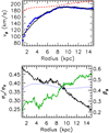 |
Fig. A.1 Top: rotation velocity curve of the simulated disk (solid black line). Filled blue symbols represent the rotation curve derived from the high-resolution mock velocity field (i = 55°, see Fig. A.3 and text). The red line indicates the circular velocity curve of the simulation. Bottom: vertical-to-radial dispersion ratio (black line) and azimuthal anisotropy (green line) of the simulated disk. The dotted line indicates the azimuthal anisotropy profile predicted by Eq. (3) of the epicyclic approximation using the circular velocity curve of the simulation. |
An artificial observed data cube is generated by projecting the position-velocity space (x,y,z,vϕ,vR,vz) of each of the 106 particles of the simulations to the sky plane, using a disk systemic velocity of 1000 km s− 1, major axis position angle of 315° (the bar being not aligned with that axis), and inclination from 35° to 75° by step of 5°. Lower and higher inclinations have not been probed to avoid the small line-of-sight contribution of the dispersions in the plane for more face-on projections, and smaller numbers of pixels for more edge-on cases. The line-of-sight projection of the velocity vector of each particle given by vlos = vsys + (vϕ cos ϕ + vR sin ϕ) sin i + vz cos i has then been assigned to a velocity channel of the data cube by interpolation. The total intensity or surface density assigned to a given pixel at a given channel is the sum of the stellar mass of each of the particles whose vlos falls within that channel. The intensity-weighted first and second moment maps of the data cube then yield mock velocity and velocity dispersion maps.
Several cases are considered to analyze the impact of the angular resolution and the noise on the results. First, high angular resolution, noise-free mock data were made assuming a distance to the galaxy of 40 Mpc and a pixel scale in the sky plane (or detector) of 1′′ (190 pc at the adopted distance). The dimensions of these mock data cubes are 512 × 512 × 141 (α,δ,vheliocentric), adopting a spectral sampling of 5 km s− 1. The high-resolution mock data is the most ideal case that is used as reference for further comparisons with the modeling at low resolution.
Then, lower angular resolution data were created to mimic observations in better agreement with CALIFA observations. The typical distance of a galaxy in CALIFA is 65 Mpc, projecting the 3″ fiber scale of the IFS instrument in a linear scale of 0.95 kpc. This is about five times less resolved than the high angular mock data. The mock low-resolution data thus assumed a galaxy distance of 65 Mpc and a pixel scale of 3″, yielding data cubes of dimensions 64 × 64 × 141, for a spectral dimension still sampled with a 5 km s−1 channel width. Furthermore, the following cases were studied at low-resolution: data with or without noise and with or without corrections from the angular effect.
The impact of noise on the anisotropy was studied by applying a noise pattern that matches the observational error on individual line-of-sight dispersion of CALIFA to the mock low angular dispersion fields. Observed dispersions are less accurate in the low regime of random motions, which occurs mainly in outer regions of galactic disks or in low mass disks. This can be explained by the combined effect of the smaller signal-to-noise in spectra from low luminosity regions with the limited spectral resolution. I defined the noise pattern by the distribution of average errors as a function of dispersion for the CALIFA subsample of 93 galaxies described of Sect. 2. This noise pattern is given in Fig. A.2 and shows that the error reaches 25% of σlos at low dispersion, while it is negligible at large dispersion. In the noisy model, each value of a noise-free dispersion map was replaced by another value randomly chosen from a normal law centered on the noise-free random motion and of standard deviation the corresponding ⟨ϵσlos∕σlosMAX⟩ value from Fig. A.2. The maximum value in the noise-free dispersion map is adopted as the normalization factor σlosMAX.
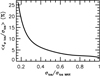 |
Fig. A.2 Noise pattern introduced in the mock data. It corresponds to the average error on stellar σlos in CALIFA as a function of line-of-sight dispersion. The σlos has been normalized to the maximum observed value of the present CALIFA sample. |
The resolution effect (also called smearing effect) stems from the observation of any velocity gradient with a finite angular sampling/resolution and generates a pattern inside a dispersion map that is not made of genuine random motions. That effect is stronger with lower angular sampling/resolution and also depends on the amplitude of the velocity gradients in the galaxies. For instance, it is more important for disks with steep inner rotation curves than with shallower curves. Also, at a given rotation curve slope, the inner structure of the dispersion pattern is more prominent at higher inclination. I modeled the pattern by creating data cubes made from the particles of the simulation orbiting with purely axisymmetric azimuthal motions (vR = vz = 0), choosing vϕ equal to the rotation curve of Fig. A.1. The resulting dispersion maps thus contain only the pattern caused by the projected rotation velocity gradient, which was then subtracted quadratically from the mock dispersion fields. Low-resolution models done with and without that correction make it possible to study the impact of the angular resolution on the anisotropy. It is worth stating that verifications that the effect has no impact on the results were carried out in the high-resolution configuration. Only results at low resolution are worth discussing hereafter.
For each disk inclination angle, fits of Eq. (1) to the dispersion fields were performed at fixed  , which was kept constant with radius and iterated within 0.1 to 1 by step of 0.05. The least-squares fits have the radial dispersion and azimuthal anisotropy as free parameters.
A.2: Results for the high angular resolution data
Figure A.3 (top row) shows an example of mock high angular stellar intensity, velocity, and velocity dispersion maps for a disk inclination of 55°. The stellar bar and spiral arms are well identified in these maps. The dispersion field also exhibits clear asymmetric features that reflect the anisotropic stellar orbits in the bar and spiral regions. The rotation curve of the mock observation is very similar to the true azimuthal velocity of the simulation (Fig. A.1). A minor difference exists in the inner regions, which is due to the effects of the perturbed kinematics inside the bar. Figure A.4 (top panel) shows the line-of-sight velocity dispersion of each individual pixel of that example inclination as a function of radius (black dots) and the corresponding azimuthally averaged dispersion profile (red open circles). The blue line corresponds to the azimuthally averaged profile of the fitted model dispersion map ( = 0.4, median ratio of the simulation). It is very consistent with the azimuthally σlos profile, showing the ability of the axisymmetric model to converge toward realistic results, and in particular to fit successfully the bulk of the random motions.
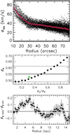 |
Fig. A.4 Illustrative results of the fitting of the dispersion model to the high-resolution i = 55 mock data. Top: line-of-sight velocity dispersion profile of the mock disk. Black dots indicate σlos in each individual pixel of the so-called observed dispersion map. The red open circles correspond to the azimuthally averaged profile of that map. The blue line corresponds to the azimuthally averaged profile of the fitted model dispersion map ( |


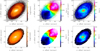 |
Fig. A.3 Example of mock line-of-sight intensity, velocity, and dispersion velocity maps of a stellar disk (from left to right, respectively). The N-body simulation of the barred spiral galaxy by Hunt et al. (2013) has been projected with an inclination of 55° and a major axis position angle of 315°, and a systemic velocity of 1000 km s− 1. The top row represents the high-resolution mock dataset (distance of 40 Mpc, spatial sampling of 1″), the bottom row the low-resolution case (distance of 65 Mpc, 3″ sampling, representative of the CALIFA resolution). |
The typical impact of  on βϕ is shown in the middle panel of Fig. A.4 for the example radius of R = 11.5 kpc. At that radius, no results could be obtained for the extreme cases
  < 0.1 and
  > 0.9. The formal errors on fitted anisotropies are negligible (0.02 at most). A narrow range of βϕ is found (0.5 ≲ βϕ ≲ 0.7), which agrees with the true value at that radius (0.53, shown as a green circle). The difference with the true value is not linear as a function of
  , but seems more consistent with a power law. In particular, derived values are more clustered at lower anisotropies and
  , thus closer to the simulated values. Consequently, it is very tempting to adopt the median value of the distribution as resulting anisotropy (solid line) and the standard deviation as resulting anisotropy uncertainty (dashed lines) at that radius.
By applying this definition to other radii, the azimuthal anisotropy profile can be recovered, making the comparison with the true simulated anisotropies possible. The bottom panel of Fig. A.4 presents the residual anisotropy profile βϕmock − βϕsim. It shows that in more than 90% of the cases the median anisotropy differs only by ∼ 0.1 at most from the true anisotropy. Larger differences occur at R ∼ 4 kpc at the end of the bar and where the inner spiral structure starts. This likely indicates a limitation of the axisymmetric model performed in this work, as in these regions the stellar kinematics is asymmetric. It is important to note that verifications were made that the modeling performed with  fixed at the true ratio in the simulation (Fig. A.1) gives results consistent with the residual anisotropy shown here.
I repeated this exercise for all high-resolution dispersion fields of different inclination, using the same disk major axis position angle and bar orientation. The distribution of anisotropy differences βϕmock − βϕsimwere then reduced to the average and standard deviation at each inclination (Fig. A.5, panel A). The impact of the inclination is to overestimate the anisotropy at low disk inclination, while it is well recovered at large inclination. However, that inclination effect is marginal as the anisotropy difference remains at the level of the standard deviation (0.1 at most). The anisotropy uncertainty on βϕ at each radius (see, e.g., the dashed lines in the middle panel of Fig. A.4) is ≲0.15 at lower inclination and ≲0.1 at larger inclination, thus in perfect agreement with the anisotropy difference within its standard deviation.
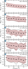 |
Fig. A.5 Residual between the fitted and simulated azimuthal anisotropy as a function of the disk inclination. The filled symbols represent the radially averaged anisotropy difference and the colored area indicates the corresponding standard deviation. For easy comparison between the various cases, the dashed lines in panels B, C, D and E delineate the colored area of panels A, B, C, D, respectively, while the dotted lines in panels B, C, D and E represent the values (symbols) of panels A, B, C, D, respectively. |
A.3: Results for the low angular resolution data
The same procedure was then applied to the low angular resolution mock data, but this time with a particular attention to understand the impact of the systematic noise and resolution effects in addition to the projection effect. Figure A.3 (bottom row) shows the example of noise-free low-resolution map (i = 55°). I followed the rule established in the modeling of CALIFA data of Sect. 2 by considering adaptive radial bins that must contain at least ten points and of minimum width of 2″. That allows successful fittings with typical formal errors on the anisotropy (standard deviation of the fitted anisotropy as a function of  at each radius) of 0.1 for most of inclinations (0.15 for inclinations closer to 35°), which agrees perfectly with errors measured at high resolution. The panel B in Fig. A.5 shows the anisotropy behavior as a function of inclination at low resolution. The inclination effect is very comparable to the high-resolution case (shown as dashed and dotted lines). The difference is the larger scatter than at high resolution, although this remains unsignificant.
The impact of the lower angular resolution can be further addressed by comparing panel C to panel B of Fig. A.5. Panel C corresponds to the low angular resolution case corrected from the resolution effect. The dispersion pattern caused by viewing the rotation curve projection at a resolution of ∼1 kpc is shown in Fig. A.6 (i = 55° case). The pattern is well identifiable by a butterfly shape of the dispersion contours, mimicking artificial anisotropy as σlos along the major and minor axes are different. Panel C shows that the azimuthal anisotropy recovered from the modeling of the mock random motion maps free from such dispersional patterns remains consistent with the simulated anisotropy. Larger differences of anisotropy still occur at low inclination and a trend for better agreement with the simulation is observed at i > 40°. The results obtained with the maps not corrected from the resolution effect remain nonetheless very comparable with the models corrected from the resolution effect within the quoted scatters.
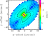 |
Fig. A.6 Dispersion pattern in the i = 55° mock dispersion velocity field caused by the effect of viewing the rotation curve at a low resolution of ∼ 1 kpc. Contours represent σlos = 2.5, 4, 5, 10, and 20 km s− 1. |
The systematic noise effect has then been addressed within panels D and E of Fig. A.5 by applying the noise model of Appendix A.3 to any inclinations and dispersion fields. Figure A.7 presents an example of residuals between the noise free and noisy mock i = 55° dispersion maps. The impact of noise is to slightly increase the scatter of the residual anisotropy, but again with no effect on the anisotropy difference. These panels also show the consistent residual and scatter for the cases with and without corrections from the resolution effect.
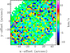 |
Fig. A.7 Residual velocity dispersion map between the noise-free and noisy mock i = 55° datasets. |
Figure A.8 presents an azimuth-dispersion diagram extracted within the example radial range R = 12 − 14 kpc for the low-resolutioncases with and without noise. This radial range was chosen to show the effect of radially biased orbits in the plane (βϕ ∼ 0.5, see Fig. A.1) on the line-of-sight dispersions. Obviously, as σϕ < σR, σlos is larger for |ϕ| → π∕2, hence closer to the minor axis than the major axis. The modeling succeeds in finding the anisotropic radial orbits (solid lines). A small difference is seen between the noisy and noise-free results in a smaller amplitude of the sine wave for the noisy case. This diagram also shows the failure of the modeling to reproduce the various dispersion wiggles through the spiral structure. This is because of the axisymmetric nature of the model of Eq. (1), which cannot produce stellar dispersions that are more asymmetric as a function of azimuth because the spiral structure is also not totally bisymmetric in that radial range. Models with high-order dispersion harmonics would certainly help in producing perturbed stellar orbits more accurately. Such an analysis is however beyond the scope of this article.
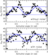 |
Fig. A.8 Azimuth-velocity dispersion diagram (low-resolution case). The top and bottom panels delineate the noise-free and noisy models, respectively. The symbols indicate the mock dispersions, and the solid lines the resulting model fitted to the mock values. The selected radial range is 12 ≤ R ≤ 14 kpc. The dashed lines highlight two extreme models of isotropic orbits, which cannot represent the intrinsinc radially biased orbits at the considered radii. |
In summary, the proposed methodology has been shown to be very appropriate in finding the bulk of the random motions and anisotropy within a large range of inclination despite the noise and resolution effects. Panel E in Fig. A.5 represents the configuration the closest to the modeling of the CALIFA velocity dispersion fields. Indeed, no attempt to correct from the resolution effect has been performed in this study owing to its very negligible impact. Random stellar motions are always significantly larger than the resolution-triggered dispersion pattern, considering that the inner slope of the stellar rotation curve of the simulated disk is of the same order of those of CALIFA stellar disks. It is worth noting in that prospect the agreement between the variation of normalized anisotropy uncertainty as a function of inclination for both the mock data and the observations (see solid line in Fig. 3).
Consequently, it is very likely that the systematic effects (inclination, resolution, and noise) make the azimuthal anisotropy measured from real galaxies with the CALIFA data, on average, different by only ∼0.1 ± 0.1 at most from reality. Both this level of systematics and the quoted formal error on anisotropy (0.1 − 0.15) remain small in comparison with the gap of anisotropy between the different families of stellar orbits in disk galaxies. In other words, a simple model like that of Eq. (1) applied to CALIFA will always be able to disentangle the different types of orbits at a resolution of 1 kpc.
Appendix B:
Negative impact of the epicyclic approximation on the vertical-to-radial axis of the velocity ellipsoid
It has been shown in Sect. 5 that Eq. (3) steming from the epicycle approximation predicts a range of anisotropy that is not representative of the diversity of orbits in CALIFA galactic planes found by Eq. (1) at free βϕ and fixed  . In this section, I use the mock data of Appendix A to carry out the opposite work that fits the model of Eq. (1) to find
  at fixed value of βϕ, by assuming that this latter is given by the epicycle theory through Eq. (3), βϕ(R) = βEA(R).
This approach was adopted by Gerssen et al. (1997, 2000), Gerssen & Shapiro Griffin (2012), Shapiro et al. (2003), or Westfall et al. (2011) and is as valid from a numerical viewpoint as the opposite approach I adopted in this study, providing that the theory is able to describe every kind of stellar orbit. However, in practice, there is no evident reason to assume that Eq. (3) should apply to any galactic disks. Indeed, at first look, it is obvious that it is possible to find tangential and isotropic orbits only at the price of continuously increasing rotation curves, which rarely occurs in reality.
In addition, although widely spread in observations, this approach has never been tested on numerical simulations. This Appendix fills that objective with the N-body model of the Milky Way-like disk.
A first step is to compare βEA with βϕ. I used the circular velocity curve of the simulation (the dashed line in top panel of Fig. A.1) to infer βEA. Not suprisingly, it yields a narrow range of values (dotted line in bottom panel of Fig. A.1) because the curve slightly increases. However, that result is not consistent with the true orbits in the simulation, which is sufficient to question the validity of the epicycle anisotropy, at least within the framework of that simulation.
Let us assume now that this disagreement applies to any observations and use this information to determine the error that is made on  when βϕ = βEA is assumed. The second step is thus to perform least-squares fits of Eq. (1) to the high-resolution mock data of Appendix A.2 at fixed βEA. Figure B.1 shows the residual profile between the mock and simulated vertical-to-radial dispersion ratios, Δz = (σz∕σR)mock − (σz∕σR)sim, for the i = 55° mock high-resolution data. With this simulation, the fitted ratio (σz∕σR)mock is significantly larger than the true values at almost every point. The difference is larger in the inner regions, which unsurprisingly corresponds to the radial range where the simulated azimuthal anisotropy differs the most from the epicycle values (Fig. A.1).
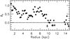 |
Fig. B.1 Residual vertical-to-radial dispersion ratio Δz = (σz∕σR)mock − (σz∕σR)sim for the i = 55° example mock data. The profile has been obtained assuming βϕ(R) = βEA(R). The quoted uncertainties are the formal errors from the fits. |
Once again, this exercise was repeated to any mock inclinations, and the average normalized differences from the true (simulated) ratio ⟨Δz∕(σz∕σR)sim⟩ were derived. The results shown in Fig. B.2 illustrate the impact on  owing to the choice of an incorrect βϕ. On the one hand, the average error is very important from 50% to 430% of the true ratio. On another hand, it strongly depends on the inclination: the more inclined, the more incorrect and the more scattered. This behavior is expected because larger inclinations leave less room to fit
  from a smaller projected contribution of σz to σlos.
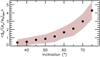 |
Fig. B.2 Residual between the fitted and simulated vertical-to-radial dispersion ratio as a function of the disk inclination. The filled symbols show the radially averaged |

Other tests to be done with larger sets of simulations would be very helpful to verify these trends, and particularly to find the conditions where βϕ ⇔ βEA and βϕ = βEA (if applicable). This work will be the subject of future papers.
Finally, I note that this does not mean that the use of the epicycle anisotropy has to be prohibited in galaxies. However, such a result illustrates nicely the dramatic consequence that the epicyclic approximation can have on the vertical ratio of stellar disks when it is known that it does not apply. As long as there is no possibility of testing if βϕ = βEA from, for example, the other approach chosen in this article, extreme caution should thus be taken when using the epicycle anisotropy to infer  from observations.
Appendix C:
Examples of results
This section shows four other examples of results for the galaxies NGC 5406, NGC 5888, UGC 08231, and UGC 09476.
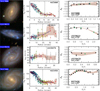 |
Fig. C.1 Examples of results with NGC 5406, NGC 5888, UGC 08231, and UGC 09476. From left to right column: composite SDSS image of the galaxy. Line-of-sight velocity dispersion profile (observation and model). Profile of stellar azimuthal anisotropy parameter (symbols and dashed area) and epicyclic anisotropy (dashed line). Color codes and symbols are the same as in Fig. 1. |
Appendix D:
Results of the MCMC linear fits
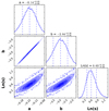 |
Fig. D.1 Results of the MCMC linear fit to the absolute magnitude-azimuthal anisotropy relation to the CALIFA stellar disks at R = h∕2 of Fig. 7. |
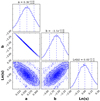 |
Fig. D.2 Results of the MCMC linear fit to the stellar mass-azimuthal anisotropy relation to the CALIFA stellar disks of Fig. 11. The anisotropy parameter that was fitted is the median of each anisotropy profile. |
All Tables
All Figures
|
Fig. 1 Example of results with the galaxy NGC 257. Top: composite SDSS image of the galaxy. Middle: line-of-sight dispersion profile. A rainbow color code is used to highlight the common spaxel centroids inside the adaptive radial rings. The shaded area represents the standard deviation of σlos inside each adaptive ring. Red open circles represent the azimuthally average of σlos within each radial ring. The thick blue line indicates the azimuthally average of the dispersion model done with |
| In the text | |
|
Fig. 2 Azimuth-velocity dispersion diagrams for 9 example galaxies. From left to right (respectively) the columns illustrate orbits that are more tangentially biased (βϕ → − 0.5), isotropic (βϕ ∼ 0), and more radially biased (βϕ → 0.5). Symbols are the CALIFA line-of-sight velocity dispersions and colored curves the best-fit anisotropic dispersion model (for the case |
| In the text | |
|
Fig. 3 Median anisotropy and uncertainty (ϵβϕ) as a function of disk inclination for the CALIFA disk galaxies. The horizontal dashed line is βϕ = 0.51 chosen by the DiskMass Survey (Bershady et al. 2011). The solid line is not a fit to the data but the uncertainty curve deduced from the mock data of Appendix A, showing the consistency between the observations and numerical modeling. |
| In the text | |
|
Fig. 4 Azimuthal anisotropy profiles for the sample of 93 CALIFA disk galaxies(circles).The filled diamonds represent the median profile derived from every galaxy and the dashed lines the standard deviation. The solid line indicates the anisotropy profile oftheMilkyWayasdeducedfromGaiaDataRelease2dispersions published in Gaia Collaboration (2018b), and an open triangle the location of the Sun. |
| In the text | |
|
Fig. 5 Median anisotropy as a function of B/T (top) and bar-to-total (bottom) luminosity fraction in the SDSS r-band. A horizontal dashed line indicates the median anisotropy of the galaxies with lower bulge contribution (bulge-to-total luminosity fraction lower than 20%). |
| In the text | |
|
Fig. 6 Azimuthal dispersion profiles color-coded with the morphological type (top) and absolute r-band magnitude (bottom). |
| In the text | |
|
Fig. 7 Absolute magnitude-anisotropy relations of CALIFA stellar disks at R = h∕2 (left) and R = h (right). Different colors and symbols represent different disk morphologies from Sa to Irr. The solid line is the most likely linear fit to βϕ (at R = h∕2 only). Crossed symbols and dotted lines represent the observed and best-fit relations predicted by the epicycle approximation for the same CALIFA disks, as deduced from circular velocity curves of Kalinova et al. (2017). Gray circles and dashed lines are the observed and best-fit relations predicted by the epicycle approximation for other galaxies, as deduced from Hα rotation curves of the GHASP sample of Epinat et al. (2008a,b). |
| In the text | |
|
Fig. 8 Hα rotation curve (vϕ, open symbols and solid line) and the epicycle anisotropy profile (βEA, dotted line) of the galaxy UGC 3809. The Hα rotation curve is from the GHASP survey (Epinat et al. 2008a,b). The solid line indicates the Einasto model of the rotation velocity. The βEA profile is deduced from the rotation model using Eq. (3). The filled circles represent βEA at R = h. |
| In the text | |
|
Fig. 9 Comparisons of stellar anisotropy βϕ and epicycle anisotropy βEA. All panels show normalized distributions in %. The bottom right panel compares the stellar anisotropy from CALIFA with the epicycle value derived from Hα rotation curves of the GHASP sample of Epinat et al. (2008a,b), while all other panels compare the stellar anisotropy from CALIFA with the epicycle value derived from CALIFA circular velocity curves of Kalinova et al. (2017). The top left graph is the total distribution of differences Δβϕ = βϕ − βEA for the 68 CALIFA galaxies with common βϕ and βEA. Blue shaded histograms are those of the stellar anisotropy, and red histograms those of the epicycle anisotropy. |
| In the text | |
|
Fig. 10 Radial profiles of difference between the stellar anisotropy βϕ and the epicycle anisotropy βEA = Δβϕ. The solid line indicates Δβϕ for the Milky Way, as derived from Gaia DR2 data published in Gaia Collaboration (2018b). The location of the Sun is indicated by a triangle. |
| In the text | |
|
Fig. 11 Stellar mass-azimuthal anisotropy correlation. The top panel shows the occurrence of galaxies per bin of stellar mass with isotropic, radial and tangential orbits (circle, triangle, and squared symbols, respectively), normalized to the total number of galaxies per 0.5 dex bin of stellar mass. The mass unit is M⊙. The starred symbol is for the Milky Way. The solid line is the most likely linear model of the mass-anisotropy relation given by Eq. (6). |
| In the text | |
|
Fig. A.1 Top: rotation velocity curve of the simulated disk (solid black line). Filled blue symbols represent the rotation curve derived from the high-resolution mock velocity field (i = 55°, see Fig. A.3 and text). The red line indicates the circular velocity curve of the simulation. Bottom: vertical-to-radial dispersion ratio (black line) and azimuthal anisotropy (green line) of the simulated disk. The dotted line indicates the azimuthal anisotropy profile predicted by Eq. (3) of the epicyclic approximation using the circular velocity curve of the simulation. |
| In the text | |
|
Fig. A.2 Noise pattern introduced in the mock data. It corresponds to the average error on stellar σlos in CALIFA as a function of line-of-sight dispersion. The σlos has been normalized to the maximum observed value of the present CALIFA sample. |
| In the text | |
|
Fig. A.4 Illustrative results of the fitting of the dispersion model to the high-resolution i = 55 mock data. Top: line-of-sight velocity dispersion profile of the mock disk. Black dots indicate σlos in each individual pixel of the so-called observed dispersion map. The red open circles correspond to the azimuthally averaged profile of that map. The blue line corresponds to the azimuthally averaged profile of the fitted model dispersion map ( |
| In the text | |
|
Fig. A.3 Example of mock line-of-sight intensity, velocity, and dispersion velocity maps of a stellar disk (from left to right, respectively). The N-body simulation of the barred spiral galaxy by Hunt et al. (2013) has been projected with an inclination of 55° and a major axis position angle of 315°, and a systemic velocity of 1000 km s− 1. The top row represents the high-resolution mock dataset (distance of 40 Mpc, spatial sampling of 1″), the bottom row the low-resolution case (distance of 65 Mpc, 3″ sampling, representative of the CALIFA resolution). |
| In the text | |
|
Fig. A.5 Residual between the fitted and simulated azimuthal anisotropy as a function of the disk inclination. The filled symbols represent the radially averaged anisotropy difference and the colored area indicates the corresponding standard deviation. For easy comparison between the various cases, the dashed lines in panels B, C, D and E delineate the colored area of panels A, B, C, D, respectively, while the dotted lines in panels B, C, D and E represent the values (symbols) of panels A, B, C, D, respectively. |
| In the text | |
|
Fig. A.6 Dispersion pattern in the i = 55° mock dispersion velocity field caused by the effect of viewing the rotation curve at a low resolution of ∼ 1 kpc. Contours represent σlos = 2.5, 4, 5, 10, and 20 km s− 1. |
| In the text | |
|
Fig. A.7 Residual velocity dispersion map between the noise-free and noisy mock i = 55° datasets. |
| In the text | |
|
Fig. A.8 Azimuth-velocity dispersion diagram (low-resolution case). The top and bottom panels delineate the noise-free and noisy models, respectively. The symbols indicate the mock dispersions, and the solid lines the resulting model fitted to the mock values. The selected radial range is 12 ≤ R ≤ 14 kpc. The dashed lines highlight two extreme models of isotropic orbits, which cannot represent the intrinsinc radially biased orbits at the considered radii. |
| In the text | |
|
Fig. B.1 Residual vertical-to-radial dispersion ratio Δz = (σz∕σR)mock − (σz∕σR)sim for the i = 55° example mock data. The profile has been obtained assuming βϕ(R) = βEA(R). The quoted uncertainties are the formal errors from the fits. |
| In the text | |
|
Fig. B.2 Residual between the fitted and simulated vertical-to-radial dispersion ratio as a function of the disk inclination. The filled symbols show the radially averaged |
| In the text | |
|
Fig. C.1 Examples of results with NGC 5406, NGC 5888, UGC 08231, and UGC 09476. From left to right column: composite SDSS image of the galaxy. Line-of-sight velocity dispersion profile (observation and model). Profile of stellar azimuthal anisotropy parameter (symbols and dashed area) and epicyclic anisotropy (dashed line). Color codes and symbols are the same as in Fig. 1. |
| In the text | |
|
Fig. D.1 Results of the MCMC linear fit to the absolute magnitude-azimuthal anisotropy relation to the CALIFA stellar disks at R = h∕2 of Fig. 7. |
| In the text | |
|
Fig. D.2 Results of the MCMC linear fit to the stellar mass-azimuthal anisotropy relation to the CALIFA stellar disks of Fig. 11. The anisotropy parameter that was fitted is the median of each anisotropy profile. |
| In the text | |
Current usage metrics show cumulative count of Article Views (full-text article views including HTML views, PDF and ePub downloads, according to the available data) and Abstracts Views on Vision4Press platform.
Data correspond to usage on the plateform after 2015. The current usage metrics is available 48-96 hours after online publication and is updated daily on week days.
Initial download of the metrics may take a while.