Quantifying the stellar ages of dynamically separated bulges and disks of CALIFA spiral galaxies

Yunpeng Jin; Ling Zhu; Stefano Zibetti; Luca Costantin; Glenn van de Ven; Shude Mao

doi:10.1051/0004-6361/202347197

Home

All issues

Volume 681 (January 2024)

A&A, 681 (2024) A95

Full HTML

Open Access

Issue		A&A Volume 681, January 2024


Article Number		A95
Number of page(s)		21
Section		Extragalactic astronomy
DOI		https://doi.org/10.1051/0004-6361/202347197
Published online		23 January 2024

A&A, 681, A95 (2024)

Quantifying the stellar ages of dynamically separated bulges and disks of CALIFA spiral galaxies

Yunpeng Jin¹, Ling Zhu¹, Stefano Zibetti², Luca Costantin³^,4, Glenn van de Ven⁵ and Shude Mao⁶^,7

¹ Shanghai Astronomical Observatory, Chinese Academy of Sciences, 80 Nandan Road, Shanghai 200030, PR China
e-mail: jyp199333@163.com; lzhu@shao.ac.cn
² INAF – Osservatorio Astrofisico di Arcetri, Largo Enrico Fermi 5, 50125 Firenze, Italy
³ Centro de Astrobiología (CSIC-INTA), Ctra de Ajalvir km 4, Torrejón de Ardoz, 28850 Madrid, Spain
⁴ INAF – Osservatorio Astronomico di Brera, Via Brera 28, 20121 Milano, Italy
⁵ Department of Astrophysics, University of Vienna, Türkenschanzstraße 17, 1180 Wien, Austria
⁶ Department of Astronomy, Tsinghua University, Beijing 100084, PR China
⁷ National Astronomical Observatories, Chinese Academy of Sciences, 20A Datun Road, Chaoyang District, Beijing 100101, PR China

Received: 15 June 2023
Accepted: 27 October 2023

Abstract

We employ a recently developed population-orbit superposition technique to simultaneously fit the stellar kinematic and age maps of 82 CALIFA spiral galaxies and obtain the ages of stars in different dynamical structures. We first evaluated the capabilities of this method on CALIFA-like mock data created from the Auriga simulations. The recovered mean ages of dynamically cold, warm, and hot components match the true values well, with an observational error of up to 20% in the mock age maps. For CALIFA spiral galaxies, we find that the stellar ages of the cold, warm, and hot components all increase with the stellar mass of the galaxies, from t_cold ~ 2.2 Gyr, t_warm ~ 2.3 Gyr, and t_hot ~ 2.6 Gyr for galaxies with stellar mass M_* < 10¹⁰ M_⊙, to t_cold ~ 4.0 Gyr, t_warm ~ 5.1 Gyr, and t_hot ~ 5.9 Gyr for galaxies with M_* > 10¹¹ M_⊙. About 80% of the galaxies in our sample have t_hot > t_cold, and the mean values of t_hot − t_cold also increase with stellar mass, from 0.7_−0.2^+0.6 Gyr in low-mass galaxies (10^8.9 M_⊙ < M_* ≤ 10^10.5 M_⊙) to 1.7_−0.2^+0.7 Gyr in high-mass galaxies (10^10.5 M_⊙ < M_* < 10^11.3 M_⊙). The stellar age is younger in disks than in bulges, on average. This suggests that either the disks formed later and/or that they experienced a more prolonged and extensive period of star formation. Lower-mass spiral galaxies have younger bulges and younger disks, while higher-mass spiral galaxies generally have older bulges, and their disks span a wide range of ages. This is consistent with the scenario in which the bulges in more massive spirals formed earlier than those in less massive spirals.

Key words: galaxies: spiral / galaxies: structure / galaxies: kinematics and dynamics / galaxies: evolution / galaxies: fundamental parameters

© The Authors 2024

Open Access article, published by EDP Sciences, under the terms of the Creative Commons Attribution License (https://creativecommons.org/licenses/by/4.0), which permits unrestricted use, distribution, and reproduction in any medium, provided the original work is properly cited.

This article is published in open access under the Subscribe to Open model. Subscribe to A&A to support open access publication.

1 Introduction

Our knowledge of galaxy structures evolves with the development of the instruments that are used in galaxy observations. The preliminary understanding of external galaxies, such as the morphology and colour, directly comes from photometric images of galaxies. Galaxies are classified into different Hubble types based on the presence of a disk, a bulge, and/or bar structures (Hubble 1926). Since the 1970s, numerous single-band surveys from the ultraviolet to the far-infrared have been carried out. They generally tell us that typical elliptical galaxies (and bulges in spiral galaxies) tend to be red, gas poor, and have no ongoing star formations, whereas the disks of spiral galaxies are usually blue, gas rich, and have distinct star formation regions (Kennicutt 1998).

Since the late 1990s, large galaxy surveys such as the Sloan Digital Sky Survey (SDSS; York et al. 2000) provided multi-band images for millions of nearby galaxies. New methods such as the spectral energy distribution fitting (SED fitting; e.g. Bolzonella et al. 2000; Walcher et al. 2011) are used to derive the stellar age across the image plane for each galaxy. Low-mass galaxies are found to be typically young, while massive galaxies are usually old (e.g. Kauffmann et al. 2003; Gallazzi et al. 2005).

Most spiral galaxies have clear negative age gradients (e.g. Bell & de Jong 2000; MacArthur et al. 2004), which indicates that the stellar populations of the bulge are older than those in the disk, while the age gradients in elliptical galaxies are usually mild or even negligible (e.g. Trager et al. 2000; Mehlert et al. 2003). It has also been found that galaxies with higher stellar velocity dispersion tend to be older (e.g. Thomas et al. 2005; Bernardi et al. 2006).

It is widely thought that bulges and disks in galaxies should be formed through different physical processes. To analyse them separately, photometric bulge-disk decomposition methods are widely used, which usually assume that the surface brightness of the bulge follows a radial profile with Sérsic index n ≳ 2 (Sersic 1968), while the surface brightness of the disk follows an exponential profile with index n = 1 (e.g. Peng et al. 2002, 2010; de Souza et al. 2004; Méndez-Abreu et al. 2008). The Sérsic index derived from the photometric decomposition is widely used to separate the classical bulges that formed via major mergers and the pseudobulges, which formed via disk instability (e.g. Fisher & Drory 2008; Weinzirl et al. 2009; Gadotti 2009). However, it may not be an appropriate diagnostic for a distinction between bulges (e.g. Graham & Worley 2008; Costantin et al. 2018; Gao et al. 2022). Recent studies have shown that the surface brightness profile of the disk may not be exactly exponential, but down-bending or up-bending in the inner or outer regions (e.g. Méndez-Abreu et al. 2017; Breda et al. 2020), which challenges the basic assumption taken in photometric decomposition. In addition, photometric decomposition provides limited information on the stellar populations of bulges and disks separately.

In recent years, Integral Field Spectroscopy (IFS) surveys such as SAURON (Bacon et al. 2001), ATLAS^3D (Cappellari et al. 2011), CALIFA (Sánchez et al. 2012), SAMI (Bryant et al. 2015), MaNGA (Bundy et al. 2015), and multiple MUSE programmes (Bacon et al. 2017) have observed thousands of nearby galaxies. IFS observations allow us to investigate the spatially resolved stellar population distribution of a galaxy (e.g. McDermid et al. 2015; González Delgado et al. 2015; Goddard et al. 2017; Li et al. 2018; Bernardi et al. 2019). The traditional photometric decomposition was then updated to a spectrophotometric decomposition method (Méndez-Abreu et al. 2019), which fits the IFS data cube and obtains the stellar populations of photometrically decomposed bulges and disks separately. Subsequent research suggested that bulges in spiral galaxies form first and have not evolved much through cosmic time, and the disks are built up later around the bulges, but do not affect them significantly (e.g. Méndez-Abreu et al. 2021). Multiple spectroscopic decomposition attempts have been made that directly separated the bulge and disk by fitting the spectra (e.g. Johnston et al. 2012, 2014; Tabor et al. 2017, 2019; Oh et al. 2020; Pak et al. 2021) based on the full spectral fitting software pPXF (Cappellari & Emsellem 2004; Cappellari 2017). These works in general found that the bulges in spiral galaxies are older, more metal rich, and rotate more slowly than the disks, while the differences in age and metallicity between bulges and disks become small or even negligible in early-type galaxies. Recent studies of spiral galaxies at intermediate redshift 0.14 < z ≤ 1 based on SHARDS (Pérez-González et al. 2013) and HST/CANDELS (Koekemoer et al. 2011; Grogin et al. 2011) data also found that the bulges in spiral galaxies are usually older than the disks, and their age difference increases with galaxy stellar mass, which was explained by two formation epochs of bulges in different galaxies (Costantin et al. 2021, 2022).

Dynamical decomposition is an alternative way to distinguish between different galaxy structures, such as bulges and disks, and it is commonly used in simulations (e.g. Correa et al. 2017; Pillepich et al. 2019; Rodriguez-Gomez et al. 2019; Du et al. 2019, 2020; Pulsoni et al. 2020). This decomposition also becomes possible for real galaxies based on Schwarzschild’s orbit-superposition method (Schwarzschild 1979, 1982, 1993) by fitting the stellar luminosity distribution and kinematic data from IFS observations. Several implementations of Schwarzschild’s method are currently in use (e.g. van den Bosch et al. 2008; Vasiliev & Valluri 2020; Neureiter et al. 2021). The triaxial Schwarzschild model developed by van den Bosch et al. (2008) was extensively used to analyse large samples of nearby galaxies from IFS observations to obtain the mass distributions and intrinsic shapes (e.g. Jin et al. 2019, 2020; Santucci et al. 2022; Pilawa et al. 2022), internal orbital structures (e.g. Zhu et al. 2018a,b,c; Jin et al. 2019, 2020; Santucci et al. 2022), and black hole masses (e.g. Quenneville et al. 2021, 2022; Pilawa et al. 2022). This triaxial model has recently been modified to explicitly include a bar (Tahmasebzadeh et al. 2021, 2022). The orbit-superposition method allows us to obtain the probability density distributions of stellar orbits in a galaxy and to carry out an orbital decomposition. Studies of CALIFA galaxies revealed that dynamically hot orbits usually occupy the inner bulge regions, while dynamically cold orbits are well correlated with the photometrically decomposed disk fraction (Zhu et al. 2018a,c). The hot orbit fraction f_hot decreases with stellar mass for galaxies with M_* < 10¹⁰ M_⊙ and increases with stellar mass for galaxies with M_* > 10¹⁰ M_⊙, while the cold orbit fraction fcoid increases with stellar mass below 10¹⁰ M_⊙ and decreases with stellar mass above 10¹⁰ M_⊙ (Zhu et al. 2018b). Similar mass dependences of f_hot and f_cold were also found in Jin et al. (2020) for MaNGA early-type galaxies. These results enabled direct and statistical comparison of galactic structures to cosmological simulations (Xu et al. 2019).

A population-orbit superposition method has further been developed based on the Schwarzschild method by tagging the stellar orbits with ages and metallicities, allowing us to obtain the stellar populations of different dynamical structures. This method was validated by Zhu et al. (2020) using MUSE-like mock data created from the Auriga simulations (Grand et al. 2017). It has been applied to 23 early-type galaxies from the Fornax3D project (Sarzi et al. 2018), leading to several new analyses of the internal galaxy structures, including the deviation of the intrinsic age-velocity dispersion profile in disks of external galaxies (Poci et al. 2019, 2021), weighting and timing ancient massive mergers in external galaxies using a so-called hot inner stellar halo structure (Zhu et al. 2022a,b), and probing the cluster environmental effects on the formation of cold galaxy disks (Ding et al. 2023).

In this paper, we validate the population-orbit superposition method with CALIFA-like mock data and apply it to a sample of 82 CALIFA spiral galaxies. With the stellar orbit distributions already derived from Zhu et al. (2018b) via the standard Schwarzschild method, we further obtain the stellar ages of different dynamical components. In Sect. 2, we introduce the population-orbit superposition method. In Sect. 3, we validate the method with CALIFA-like mock data, and in Sect. 4 we present the statistical analysis for CALIFA spiral galaxies. We discuss our findings in Sect. 5, and we conclude in Sect. 6.

2 The population-orbit superposition method

We took a two-step process to create a population-orbit superposition model for a galaxy, as proposed by Zhu et al. (2020): We first created a standard Schwarzschild’s orbit-superposition model by fitting the stellar luminosity distribution and kinematic data, and searched for the best-fitting model by exploring the free parameter space. Then we tagged the stellar orbits of the best-fitting model with stellar populations. In this paper, we only tagged stellar orbits with stellar ages, but not with metallicities.

2.1 Creating an orbit-superposition model

This paper follows the same approach as van den Bosch et al. (2008) and Zhu et al. (2018b). We took three steps to create an orbit-superposition Schwarzschild model for a galaxy: (1) We constructed the gravitational potential, (2) sampled and integrated orbits, and (3) solved the orbit weights by fitting the observational data, which included the 2D surface brightness, the 3D luminosity density distribution, and kinematic data.

The gravitational potential of the galaxy was generated by combining a triaxial stellar component, a dark matter halo, and a central supermassive black hole that was treated as a point source. To calculate the stellar potential, the galaxy surface brightness was first fitted by the multi-Gaussian expansion (MGE) formalism (Emsellem et al. 1994; Cappellari 2002).

The 3D luminosity density was then deprojected from the 2D MGE by setting the viewing angles (θ, ϕ,ψ). By multiplying the 3D luminosity density by the mass-to-light ratio M_*/L, the stellar mass distribution was calculated, and subsequently the stellar gravitational potential was derived by solving Poisson’s equation. The dark matter potential was described by a spherical Navarro-Frenk-White (NFW) profile (Navarro et al. 1996), which had two free parameters: the enclosed halo mass M₂₀₀ within the virial radius, and the dark matter concentration c. The viewing angles (θ, ϕ,ψ) were transformed into the intrinsic triaxial shapes of the galaxy: the axis ratios p = b/a, q = c/a, and the compression factor u. In practice, to reduce degeneracy, the concentration c was fixed following the M₂₀₀ − c relation from Dutton & Macciò (2014), and the compression factor was set to u = 0.9999. Thus, there were four free parameters in total: M_*/L, p, q, and M₂₀₀.

The orbits were sampled from three integrals of motion that define a triaxial system: energy E, second integral I₂, and third integral I₃. The orbit libraries include a typical library of orbits sampled from the x − z plane, a library of counter-rotating orbits, and an additional library of box orbits sampled from the equipotential plane. When modelling CALIFA galaxies (Zhu et al. 2Ol8b,c), a combination of 21 × 10 × 7 intervals in (E, I₂, I₃) was used to generate the initial orbit conditions in each orbit library. Then, by slightly perturbing the initial conditions, each orbit was dithered to 5³ orbits to form an orbit bundle. Thus, there are 3 × 21 × 10 × 7 = 4410 orbit bundles in total.

The orbit weights were then solved using the non-negative least-squares (NNLS; Lawson & Hanson 1974) implementation, taking both stellar luminosity distribution and kinematic data as constraints. The $χ_{err}^{2}$ $\chi _{{\rm{err}}}^2$ that needs to be minimised by NNLS is expressed as

$χ_{err}^{2} = χ_{lum}^{2} + χ_{kin}^{2} .$ $\chi _{{\rm{err}}}^2 = \chi _{{\rm{lum}}}^2 + \chi _{{\rm{kin}}}^2.$ (1)

For the luminosity distribution, we used both the 2D surface brightness and 3D luminosity density as constraints. The 2D surface brightness was stored in the same apertures as the kinematic data, with S _i representing the surface brightness in the ith aperture. The 3D space was divided into 360 cells, with γ_m representing the luminosity of the mth cell. We set the relative errors of S_i to be 1% and γ_m to be 2%. For the kinematic data, we fit the Gauss–Hermite coefficients (Gerhard 1993; van der Marel & Franx 1993; Rix et al. 1997) of the line-of-sight velocity distribution. The Gauss-–Hermite coefficients and their errors h₁, h₂, Δh₁, and Δh₂ were converted from the observational data V, σ, ΔV, and Δσ. Thus, we have

$χ_{lum}^{2} = \sum_{i = 1}^{N_{obs}} {(\frac{S_{i}^{*} - S_{i}}{0.01 S_{i}})}^{2} + \sum_{m = 1}^{M} {(\frac{γ_{m}^{*} - γ_{m}}{0.02 γ_{m}})}^{2},$ $\chi _{{\rm{lum}}}^2 = \sum\limits_{{\rm{i}} = 1}^{{N_{{\rm{obs}}}}} {{{\left( {{{S_i^* - {S_i}} \over {0.01{S_i}}}} \right)}^2}} + \sum\limits_{{\rm{m}} = 1}^M {{{\left( {{{\gamma _m^* - {\gamma _m}} \over {0.02{\gamma _m}}}} \right)}^2}} ,$ (2)

$\begin{array}{l} χ_{lum}^{2} = \sum_{i = 1}^{N_{obs}} [{(\frac{h_{1 i}^{*} - h_{1 i}}{Δ h_{1 i}})}^{2} + {(\frac{h_{2 i}^{*} - h_{2 i}}{Δ h_{2 i}})}^{2} \\ + {(\frac{h_{3 i}^{*} - h_{3 i}}{Δ h_{3 i}})}^{2} + {(\frac{h_{4 i}^{*} - h_{4 i}}{Δ h_{4 i}})}^{2}], \end{array}$ $\matrix{ {\chi _{{\rm{lum}}}^2 = \sum\limits_{{\rm{i}} = 1}^{{N_{{\rm{obs}}}}} {\left[ {{{\left( {{{h_{1i}^* - {h_{1i}}} \over {{\rm{\Delta }}{h_{1i}}}}} \right)}^2} + {{\left( {{{h_{2i}^* - {h_{2i}}} \over {{\rm{\Delta }}{h_{2i}}}}} \right)}^2}} \right.} } \hfill \cr {\,\,\,\,\,\,\,\,\,\,\,\,\,\,\,\,\left. {\,\,\, + {{\left( {{{h_{3i}^* - {h_{3i}}} \over {{\rm{\Delta }}{h_{3i}}}}} \right)}^2} + {{\left( {{{h_{4i}^* - {h_{4i}}} \over {{\rm{\Delta }}{h_{4i}}}}} \right)}^2}} \right],} \hfill \cr }$ (3)

where N_obs is the number of 2D apertures, and M is the number of 3D cells. Variables marked with an asterisk indicate the model fittings, those with an upward-pointing triangle represent the errors of the input data, and those without a marker denote the input data.

After solving the orbit weights, we calculated the difference between model-recovered and observed kinematic maps directly,

$\begin{array}{l} χ^{2} = \sum_{i = 1}^{N_{obs}} [{(\frac{V_{i}^{*} - V_{i}}{Δ V_{1 i}})}^{2} + {(\frac{σ_{i}^{*} - σ_{i}}{Δ σ_{i}})}^{2} \\ + {(\frac{h_{3 i}^{*} - h_{3 i}}{Δ h_{3 i}})}^{2} + {(\frac{h_{4 i}^{*} - h_{4 i}}{Δ h_{4 i}})}^{2}], \end{array}$ $\matrix{ {{\chi ^2} = \sum\limits_{{\rm{i}} = 1}^{{N_{{\rm{obs}}}}} {\left[ {{{\left( {{{V_i^* - {V_i}} \over {{\rm{\Delta }}{V_{1i}}}}} \right)}^2} + {{\left( {{{\sigma _i^* - {\sigma _i}} \over {{\rm{\Delta }}{\sigma _i}}}} \right)}^2}} \right.} } \hfill \cr {\,\,\,\,\,\,\,\,\,\,\,\,\,\,\,\,\left. { + {{\left( {{{h_{3i}^* - {h_{3i}}} \over {{\rm{\Delta }}{h_{3i}}}}} \right)}^2} + {{\left( {{{h_{4i}^* - {h_{4i}}} \over {{\rm{\Delta }}{h_{4i}}}}} \right)}^2}} \right],} \hfill \cr }$ (4)

which, in principle, should be highly correlated with $χ_{kin}^{2}$ $\chi _{{\rm{kin}}}^2$ we fitted. However, if the line-of-sight velocity distribution significantly deviates from a Gaussian distribution,; $χ_{kin}^{2}$ $\chi _{{\rm{kin}}}^2$ and; χ² may not be similar. Because; χ² directly reflects how the model matches the data, we took χ² to represent the goodness of fit. In practice, luminosity distributions are much easier to fit than kinematic data, so that $χ_{lum}^{2}$ $\chi _{{\rm{lum}}}^2$ is a low value and was not taken into account in the goodness evaluation.

We have four free hyper-parameters (M_*/L, p, q, and M₂₀₀), and we took an iterative process to search for the best-fitting model. We started by making initial guesses of the parameters. After constructing the initial models, we selected the models within a relatively lower χ² and created new models around these selected models by walking a few steps in the parameter space. We initially took large step sizes of 0.1, 0.05, 0.05, and 0.5 for M_*/L, p, q, u, and M₂₀₀/M_* to avoid becoming stuck in a local minimum. We repeated this iterative process until we reached a minimum χ² with all models around it calculated in the parameter space. Then we reduced the step size to half and repeated the process again. Finally, we determined the model with the minimum χ², and all the models around it in the parameter space within 3σ confidence level were calculated.

In the end, we not only constrained the free parameters in the potential, but also obtained the best-fitting model whose stellar orbit distribution is representative of the real galaxy. Following Zhu et al. (2018b,c), we characterised each orbit by its time-averaged radius r and circularity λ_z. Circularity λ_z represents the angular momentum of the orbit around the short axis normalised by the maximum of a circular orbit with the same binding energy. Therefore, we obtained the probability density distributions of stellar orbits in the phase space of λ_z versus r, as illustrated in Fig. 1, taking a typical simulated spiral galaxy as an example.

2.2 Tagging the stellar orbits with ages

After obtaining the best-fitting model in the previous step, we tagged the stellar orbits of the best-fitting model with stellar ages. We took the basic assumption that the stars on similar orbits have similar stellar populations. Following Zhu et al. (2020), we divided the orbits in λ_z-r phase space into different bundles using the Voronoi 2D binning method (Cappellari & Copin 2003), ensuring that each bundle contained at least 0.5% of the total orbit weight, which resulted in N_b ~ 100 orbit bundles, as illustrated in Fig. 1. We assumed that stars in the same orbit bundle are represented by a simple stellar population of age t_k to be determined. Then we tagged the orbit bundles with ages, projected them onto the observing plane, and extracted a map of the stellar ages. The age $t_{model}^{i}$ $t_{{\rm{model}}}^i$ of each aperture i in the observing plane was calculated by

$t_{model}^{i} = \frac{\sum_{k = 1}^{N_{b}} t_{k} f_{k}^{i}}{\sum_{k = 1}^{N_{b}} f_{k}^{i}},$ $t_{{\rm{model}}}^i = {{\sum\nolimits_{k = 1}^{{N_{\rm{b}}}} {{t_k}f_k^i} } \over {\sum\nolimits_{k = 1}^{{N_{\rm{b}}}} {f_k^i} }},$ (5)

where N_b is the total number of orbit bundles, and $f_{k}^{i}$ $f_k^i$ is the luminosity contributed by the orbit bundle k in aperture i. The age t_k of each orbit bundle could be solved by matching the model-predicted age map with the observed data.

We adopted a Bayesian analysis to match the model-predicted age $t_{model}^{i}$ $t_{{\rm{model}}}^i$ with the observational age map $t_{obs}^{i}$ $t_{{\rm{obs}}}^i$ . To do this, we employed the Python package PyMC3¹, which is a probabilistic programming library that allows users to build Bayesian models and fit them with Markov chain Monte Carlo (MCMC) methods. This package allows us to approximate the posterior likelihoods, and here we adopted the Student T distribution. We began the MCMC chain with an age of $t_{k}^{start}$ $t_k^{{\rm{start}}}$ , which was sampled from a bounded Gaussian distribution,

$t_{k}^{start} ~ N (μ_{k}, σ_{k}, [0, 14]),$ $t_k^{{\rm{start}}}\~N\left( {{\mu _k},{\sigma _k},\left[ {0,14} \right]} \right),$ (6)

where µ_k is the centre of the Gaussian, and σ_k represents the dispersion. We set the physical restriction that the age value must be between 0 and 14 Gyr. The starting values of age $t_{k}^{start}$ $t_k^{{\rm{start}}}$ were initialised using the method called automatic differentiation variational inference (Advi) with 200 000 draws. Then we ran 2000 steps and took the mean age of the last 500 steps as t_k of each orbit bundle.

Because our aim is to probe the internal 3D age distribution constrained by the 2D age map with limited data quality such as CALIFA, the age of stellar orbit t_k may not be fully constrained by the data, but may be affected by the starting values $t_{k}^{start}$ $t_k^{{\rm{start}}}$ in the Bayesian analysis. In the next section, we discuss the effects of choosing different µ_k and σ_k.

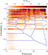Fig. 1

Probability density distributions of stellar orbits P(λ_z, r) in the phase space of time-averaged radius r vs. circularity λ_z for the best-fitting model of a typical simulated spiral galaxy. The normalized probability P/P_max is indicated by the colour bar. We adopted the Voronoi-binning scheme in the λ_z-r plane to make roughly equal-weight orbit bundles. Their boundaries are represented by the blue lines.

3 Method validation with mock data

3.1 The Auriga simulations

The Auriga project is a suite of cosmological magnetohydro-dynamical zoom-in simulations, which consists of 30 isolated Milky Way-mass haloes (Grand et al. 2017). The Auriga sample was selected from the dark matter-only version of the EAGLE Ref-L100N1504 simulation (Schaye et al. 2015), and the simulations were carried out with the N-body magnetohy-drodynamical moving-mesh code AREPO (Springel 2010). The simulations contain comprehensive physical processes of galaxy formation, such as primordial and metal-line cooling mechanism (Vogelsberger et al. 2013), a hybrid multi-phase star formation model (Springel & Hernquist 2003), stellar feedback (Marinacci et al. 2014), AGN feedback (Springel et al. 2005), a UV background field (Faucher-Giguère et al. 2009), and magnetic fields (Pakmor & Springel 2013). The initial masses of baryon particles and high-resolution dark matter particles were m_b ~ 5 × 10⁴ M_⊙ and m_DM ~ 3 × 10⁵ M_⊙, respectively. We refer to Grand et al. (2017) for more details of the Auriga simulations.

3.2 Mock data

In this paper, we selected the three simulated galaxies Au-5, Au-6, and Au-23 from Auriga with different stellar masses M_*, dark matter halo masses M₂₀₀, and structures. Both Au-5 (M_* = 6.7 × 10¹⁰ M_⊙, M₂₀₀ = 1.2 × 10¹² Mo) and Au-6 (M_* = 4.75 × 10¹⁰ M_⊙, M₂₀₀ = 1.0 × 10¹² M_⊙) have spiral arms and a weak bar in their structures, while Au-23 (M_* = 9.02 × 10¹⁰ M_⊙, M₂₀₀ = 1.45 × 10¹² M_⊙) has warps and a strong bar. For each simulation, we created three versions of mock data with inclination angles ranging from close to face-on to close to edge-on: ϑ = 40°, 60°, and 80°.

We projected each simulated galaxy onto the observational plane with a particular inclination angle ϑ, placed it at a distance of 80 Mpc, and observed it as a real galaxy. We first observed it with a pixel size of 1 arcsec and calculated the stellar mass of the particles in each pixel to obtain a surface mass density map. Then we created mock stellar kinematic and age maps with a spatial coverage and resolution similar to those of the data from CALIFA survey. For each pixel, we calculated signal-to-noise ratio (S/N) by taking the particle numbers as the signal and assuming Poisson noise. Then we performed the Voronoi-binning scheme to obtain apertures with their sizes similar to those of CALIFA galaxies, which was accomplished by setting a target S/N = 50 with the Auriga simulation. For each aperture, we calculated the flux and the line-of-sight velocity distribution, and fit the latter with a Gauss–Hermite distribution. We thus obtained the mean velocity V, the velocity dispersion σ, the skewness h₃, and the kurtosis h₄. We note that the binned target S /N = 50 is higher than the S/N of CALIFA data. We further perturbed the kinematic data by adding random noise following the method in Tsatsi et al. (2015), so that the uncertainties of the perturbed kinematic data were similar to those of the CALIFA data.

We took each mock data set as an observed galaxy and created the orbit-superposition model to fit the data. In Fig. 2 we show Au-6 with an inclination angle ϑ = 60^° as an example to demonstrate the mock data, the best-fitting model, and their residuals.

We constructed the age maps using the same binning scheme as for the kinematic maps. We first calculated the mass-weighted mean age tⁱ of the particles in each aperture i and then added the Gaussian-distributed relative errors to the ages. Thus, the observational age map $t_{obs}^{i}$ $t_{{\rm{obs}}}^i$ and the error map $t_{obserr}^{i}$ $t_{{\rm{obserr }}}^i$ were written as

$\begin{array}{l} t_{obs}^{i} = t^{i} + t^{i} \times N (0, x), \\ t_{obserr}^{i} = x \times t^{i}, \end{array}$ $\matrix{ {t_{{\rm{obs}}}^i = {t^i} + {t^i} \times N\left( {0,x} \right),} \hfill \cr {t_{{\rm{obserr}}}^i = x \times {t^i},} \hfill \cr }$ (7)

where N(0, x) denotes the Gaussian distribution with centre 0 and dispersion x. Here, x represents the relative error of the age map, and we took x = 5%, 10%, 15%, and 20% in our analysis. By creating four versions of the age maps with different errors, we finally had 3 × 3 × 4 = 36 mock age data sets. We used Au-6 with an inclination ϑ = 60° and an error of 5% of the age map (denoted Au-6-60-5 hereafter) to illustrate our method and results.

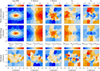Fig. 2

Mock surface brightness, stellar kinematic data, and best-fitting model for Au-6 with an inclination angle ϑ = 60°. From left to right: logarithmic normalised surface brightness, mean velocity V, velocity dispersion σ, skewness h₃, and kurtosis h₄. From top to bottom: mock observations, model fittings, and residuals. The residuals represent the relative deviations of the surface brightness and the standardised residuals of the kinematics.

3.3 Priors of the Bayesian analysis

For each mock data set, we first obtained the stellar orbit distribution by fitting the luminosity distribution and kinematic data. We then adopted a Bayesian analysis to fit the mock age map. Recent works have shown that stellar ages are strongly correlated with stellar kinematics in both real observations (e.g. Zhu et al. 2022a) and simulations (e.g. Trayford et al. 2019; Bird et al. 2013; Stinson et al. 2013). Old stars are usually dominated by random motion, while young stars tend to form a rotation-dominated disk. Therefore, we used the correlation between the stellar age and the orbit circularity to set the prior of the stellar age of the orbit.

3.3.1 Single-age prior: Model A

Following Zhu et al. (2020), we determined the age-circularity prior by iterative model fitting. We first started the PyMC3 procedure with a uniform prior, where (µ_k, σ_k) were set to the mean value and twice the standard deviation of the observational age map,

$\begin{array}{l} μ_{k} = 〈 t_{obs}^{i} 〉, \\ σ_{k} = 2 σ (t_{obs}^{i}) . \end{array}$ $\matrix{ {{\mu _k} = \left\langle {t_{{\rm{obs}}}^i} \right\rangle ,} \hfill \cr {{\sigma _k} = 2\sigma \left( {t_{{\rm{obs}}}^i} \right).} \hfill \cr }$ (8)

Then we processed a linear fitting to the outcome t_k(λ_z) from the previous model and took the fitting results as a new prior,

$\begin{array}{l} μ_{k} = t_{λ_{z} = 0} + (t_{λ_{z} = 1} - t_{λ_{z} = 0}) λ_{z}, & if & λ_{z} \geq 0; \\ μ_{k} = t_{λ_{z} = 0}, & if & λ_{z} < 0; \\ σ_{k} = 2 σ (t_{obs}^{i}) . \end{array}$ $\matrix{ {{\mu _k} = {t_{{\lambda _z} = 0}} + \left( {{t_{{\lambda _z} = 1}} - {t_{{\lambda _z} = 0}}} \right){\lambda _z},} \hfill & {{\rm{if}}} \hfill & {{\lambda _z} \ge 0;} \hfill \cr {{\mu _k} = {t_{{\lambda _z} = 0}},} \hfill & {{\rm{if}}} \hfill & {{\lambda _z} < 0;} \hfill \cr {{\sigma _k} = 2\sigma \left( {t_{{\rm{obs}}}^i} \right).} \hfill & {} \hfill & {} \hfill \cr }$ (9)

Here, µ_k equals a constant value when λ_z < 0, and follows a linear relation with the circularity λ_z when λ_z > 0. We reran the model with the refined prior from the previous model iteratively. The results usually converged after one or two iterations. We took the average ages of the last 500 steps in the MCMC chains from the last model iteration as our final results. In Fig. 3 we show how the prior µ_k is refined in a model of Au-6-60-5. The scatter between the final results and the refined prior is correlated with σ_k. We call this iterative model model A.

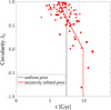Fig. 3

Correlation between stellar age t and circularity λ_z demonstrated with Au-6-60-5. The dotted black line represents µ_k of the uniform prior we started with, while the solid red line represents µ_k of the iteratively refined prior based on the results from the previous model run. The red dots represent the final t_k obtained in the last model iteration. Larger dot sizes indicate larger orbit weights of the orbit bundles.

3.3.2 Multiple age priors: Model B

With limited data quality, we tried to improve the recovery of the stellar age distributions by introducing a revised model, model B. This model followed the same linear relation as model A, but allowed different values of $t_{λ_{z} = 0}, t_{λ_{z} = 1}$ ${t_{{\lambda _z} = 0}},{t_{{\lambda _z} = 1}}$ and σ_k. We set $t_{λ_{z} = 0}$ ${t_{{\lambda _z} = 0}}$ and $t_{λ_{z} = 1}$ ${t_{{\lambda _z} = 1}}$ to range from 0.25 to 13.75 Gyr with an interval of 0.75 Gyr, and σ_k to range from 0.5 to 5 Gyr with an interval of 0.5 Gyr. Because we expect the bulges to be older than the disks for most galaxies, we added an additional restriction that the priors should satisfy $t_{λ_{z} = 0} \geq t_{λ_{z} = 1}$ ${t_{{\lambda _z} = 0}} \ge {t_{{\lambda _z} = 1}}$ . In Fig. 4 we show the parameter space of ( $t_{λ_{z} = 0}$ ${t_{{\lambda _z} = 0}}$ , $t_{λ_{z} = 1}$ ${t_{{\lambda _z} = 1}}$ , σ_k), taking Au-6-60-5 as an example. For each set of priors, we created a population-orbit superposition model and calculated the $χ_{age}^{2}$ $\chi _{{\rm{age }}}^2$ between the mock age map and the corresponding model fitting,

$χ_{age}^{2} = \sum_{i = 1}^{N_{obs}} {(t_{obs}^{i} - t_{model}^{i})}^{2},$ $\chi _{{\rm{age}}}^2 = \sum\limits_{i = 1}^{{N_{{\rm{obs}}}}} {{{\left( {t_{{\rm{obs}}}^i - t_{{\rm{model}}}^i} \right)}^2}} ,$ (10)

where N_i indicates the number of apertures of age map. We used $χ_{\min^{2}}$ ${\chi _{{{\min }^2}}}$ represent the minimum $χ_{age}^{2}$ $\chi _{{\rm{age }}}^2$ in all sets of prior and defined the 1er confidence level as

$χ_{age}^{2} - χ_{min}^{2} < χ_{CL}^{2} = \sqrt{2 N_{obs}} .$ $\chi _{{\rm{age}}}^2 - \chi _{{\rm{min}}}^2 < \chi _{{\rm{CL}}}^2 = \sqrt {2{N_{{\rm{obs}}}}} .$ (11)

We averaged the age distributions of all models within the 1σ confidence level in the phase space of λ_z versus t and took this smoothed age distribution as the result from model B.

In Fig. 5, we show the best-fitting models from models A and B for Au-6-60-5. Models A and B both fit the age map well, with a relatively old inner region (t ~ 9 Gyr) and a relatively young disk (t ~ 6 Gyr). The standardised residuals between the mock observations and the model fittings are smaller than unity for more than half of the apertures.

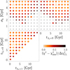Fig. 4

Parameter space of the age-circularity priors for Au-6-60-5. We use three parameters to determine the λ_z−t prior, including the age when λ_z = 0, the age when λ_z = 1, and the dispersion σ_k. The largest orange triangles denote the model with the minimum χ², and the other coloured dots represent the models within the 1σ confidence level, as indicated by the colour bar. The small black asterisks represent the models outside the 1σ confidence level.

3.4 Test results

In this subsection, we analyse the results obtained from our simulation tests in detail, including a comparison between models A and B. We show the orbit probability density distributions in the phase space of circularity λ_z versus age t for Au-6-60-5 in Fig. 6. From left to right, the true distribution directly derived from the stellar particles in the simulation is shown, followed by the model-recovered distribution from model A and that from model B. For a fair comparison, only the stellar particles within the mock data coverage are included. Model B is smoother than model A, as model B is an average of different models, while model A is just a single model. By dividing the particles or orbits into multiple circularity bins and calculating the mean age of the particles or orbits in each bin, we find that the mean age as a function of circularity from both model A and model B generally match the true one from simulations. Despite the limited data quality, both models recover the mean age as a function of circularity well, but the detailed distribution of stellar ages is not fully recovered. For example, young stars with t < 3 Gyr are not well represented by our models.

To quantify the test results, we divided each galaxy into three coarse components: cold (λ_z > 0.8), warm (0.25 < λ_z < 0.8), and hot (λ_z < 0.25), as illustrated in Fig. 6. The hot component here includes the counter-rotating (λ_z < −0.25) orbits as defined in Zhu et al. (2Ol8a,b,c). We then calculated the true and model recovered mean age of each component for all mock data sets, and we present them in Fig. 7. The middle and bottom panels show our results from model A and model B, respectively, with the relative observational error ranging from 5% to 20%. We also show the results from Zhu et al. (2020) in the top left panel. They applied model A to mock data with a MUSE-like spatial resolution.

When the observational error is 5%, model A is able to recover the mean age of each component well, similar to the results from MUSE-like mock data (Zhu et al. 2020). However, with increasing observational error, the estimations of the age of the cold and hot components (t_cold,model and t_hot,model) in model A become more biased. For the mock age maps with an observational error of 5%, 10%, 15%, and 20%, the models overestimate the mean age of the cold component by t_cold,model − t_cold,true = 0.8, 0.9, 1.0, and 1.2 Gyr and underestimate the mean age of the hot component by t_hot,model − t_hot,true = −0.3, −0.6, −0.8, and −1.3 Gyr, respectively. Model A, which started from a uniform prior, has a weak ability to distinguish the ages of different components when the observational error is as large as 20%.

The results of model B are shown in the bottom panels of Fig. 7. The mean biases of the recovered ages are within 0.3 Gyr for the cold components and within 0.7 Gyr for the hot components, with up to 20% observational error. These biases are much smaller than those of model A, and the statistical uncertainties of model B are also generally smaller. These results indicate that model B is more effective than model A, especially for data with relatively large observational errors. In both models, the ages of the cold, warm, and hot components are recovered similarly well for galaxies with different inclination angles (40°, 60°, and 80°).

When modelling real galaxies such as the CALIFA galaxies, we used the test results with an observational error of 20% to estimate the overall uncertainties of the ages of different components. We converted the absolute overall uncertainties, which included the statistical uncertainty and the mean systematic bias as shown in Fig. 7, into the relative ones. Model A has a statistical uncertainty of σ_stat = 11%, 3%, and 8% and a systematic bias of $\bar{𝒟} = 25 %$ $\overline D = 25\%$ , −9%, and −14% for the cold, warm, and hot components, respectively. Model B has a statistical uncertainty of σ_stat = 8%, 2%, and 7%, and a systematic bias of $\bar{𝒟} = 14 %$ $\overline D = 14\%$ , −9%, and −3%.

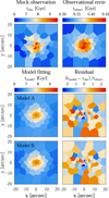Fig. 5

Mock age map and best-fitting models for Au-6-60-5. Top panels: mock age map t_obs and mock error map t_obserr. Middle panels: best-fitting age map t_model and standardised residuals between mock observations and model fittings t_stdres = (t_model − t_obs)/t_obserr derived from model A. Bottom: similar to the middle panels, but derived from model B.

4 CALIFA spiral galaxies

4.1 CALIFA survey and dynamical models

The Calar Alto Legacy Integral Field Area Survey (CALIFA; Sánchez et al. 2012) is an IFS survey that was designed to observe different types of galaxies representative of the Local Universe. Data were derived with the spectrophotometer PMAS (Roth et al. 2005) in the PPAK mode (Verheijen et al. 2004; Kelz et al. 2006) mounted on the 3.5-m telescope at the Calar Alto Observatory. The final data release (DR3; Sánchez et al. 2016) contains observations of over 600 galaxies spanning all morphological types with redshift 0.005 < z < 0.03 in the Local Universe. This release also provides stellar kinematics extracted from the medium-resolution V1200 setup and the r-band images from SDSS DR8 (Aihara et al. 2011) for an ensemble of 300 galaxies with the stellar mass range from 10^8.7 to 10^11.9 M_⊙. These 300 CALIFA galaxies were modelled using the triaxial Schwarzschild code implemented by van den Bosch et al. (2008), and the stellar orbit distributions of these CALIFA galaxies were then derived from the models (Zhu et al. 2018b). A bug in this triaxial Schwarzschild code was recently reported (Quenneville et al. 2022), but the stellar orbit distributions based on the original code should not be affected (Thater et al. 2022). Thus, we directly used the best-fitting models from Zhu et al. (2018b) in our work.

4.2 Stellar age maps and sample selection

The stellar age maps we used originally came from Zibetti et al. (2017). They derived the stellar population properties of CALIFA galaxies based on a set of five spectral indices and the photometric fluxes in the five SDSS bands, using a Bayesian approach similar to that of Gallazzi et al. (2005). We matched the catalogues from Zhu et al. (2018b) and Zibetti et al. (2017) and obtained 227 galaxies with both complete standard orbit-superposition models and observational age maps, including 160 spiral galaxies and 67 early-type galaxies. We further excluded spiral galaxies with fewer than 30 apertures in their kinematic maps, which resulted in 113 spiral galaxies with guaranteed data quality and reliable stellar orbit distributions from the orbit-superposition model. We then removed those with obvious asymmetric features in the age maps inspected by eye because our model is point-symmetrised and can never match the asymmetric features. In the end, we obtained a final sample of 82 spiral galaxies with their stellar mass ranging from 10^8.9 to 10^11.3 M_⊙. The surface brightness profiles of our sample within different mass bins are shown in Fig. A.1, and the age profiles of our sample are shown in Fig. A.2. Most of the spiral galaxies in our final sample have negative age gradients. We calculated the luminosity-weighted mean age within and outside half the effective radius R_e/2 and found that 94% of the galaxies are older in the inner regions and younger in the outer regions. This suggests that the bulges in spiral galaxies, which are spatially concentrated, are mostly older than the disks, which are extended. The 67 early-type galaxies lack obvious age gradients statistically, and we did not tag their orbits with ages. We mention them in the discussion section when we compare with the main results from spiral galaxies by directly taking the average age of the whole galaxy as the age of the bulge.

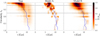Fig. 6

Probability density distributions of stellar orbits P(λ_Z, t) in the phase space of circularity λ_z vs. age t for Au-6-60-5. Left panel: true distribution directly derived from the simulation. Middle panel: model-recovered distribution from model A. Right panel: model-recovered distribution from model B, which is the average of all acceptable models within the 1σ confidence level. The normalised probability P/P_max is indicated by the colour bar. The horizontal dashed lines divide the cold (λ_z ≥ 0.8), warm (0.25 < λ_z < 0.8) and hot (λ_z ≤ 0.25, including the counter-rotating orbits) components. The solid blue line in each panel represents the mean stellar age as a function of circularity from the simulations, while the dashed blue lines denote the model-recovered ages from models A and B.

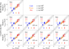Fig. 7

One-to-one comparison of the true and model-recovered age of the cold, warm, and hot orbit components for all mock data sets. Top left panel: results using model A and mock data with a MUSE-like spatial resolution from Zhu et al. (2020). Middle panels: results using model A and mock data with a CALIFA-like spatial resolution. Bottom panels: results using model B and mock data with a CALIFA-like spatial resolution. In the middle and bottom panels, the relative observational errors equal 5%, 10%, 15%, and 20% from left to right. The triangles, squares, and circles represent the mock data sets with inclination angles of 40°, 60°, and 80°. Blue, orange, and red markers denote the cold (λ_z > 0.8), warm (0.25 < λ_z < 0.8), and hot (λ_z ≤ 0.25) components. Their corresponding mean bias and statistical uncertainty are shown by the coloured texts and error bars in each panel. The dashed lines represent the equality of t_model and t_true, while the dotted lines are ±1 Gyr away from the dashed lines.

4.3 Fitting the stellar age maps

For each of the 82 spiral galaxies, we took the best-fitting orbit-superposition model and tagged stellar ages to the orbits. Before fitting the age map, we first binned the age map to reduce the high-frequency noise. For each pixel j in a galaxy, an r-band luminosity-weighted mean stellar age t_j together with its uncertainty σ(t_j) was calculated by Zibetti et al. (2017). Following the same spatial binning scheme as the kinematic map, the luminosity-weighted binned age could be written as

$t_{obs}^{i} = \frac{\sum_{j = 1}^{N_{i}} L_{j} t_{j}}{\sum_{j = 1}^{N_{i}} L_{j}},$ $t_{{\rm{obs}}}^i = {{\sum\nolimits_{j = 1}^{{N_i}} {{L_j}{t_j}} } \over {\sum\nolimits_{j = 1}^{{N_i}} {{L_j}} }},$ (12)

where L_j is the r-band luminosity of pixel j, and N_i represents the number of pixels in aperture i. Thus, the characteristic error of the binned age could be calculated by

$t_{obserr}^{i} = \frac{\sqrt{\sum_{j = 1}^{N_{i}} L_{j}^{2} σ {(t_{j})}^{2}}}{\sum_{j = 1}^{N_{i}} L_{j}} .$ $t_{{\rm{obserr}}}^i = {{\sqrt {\sum\nolimits_{j = 1}^{{N_i}} {L_j^2\sigma {{\left( {{t_j}} \right)}^2}} } } \over {\sum\nolimits_{j = 1}^{{N_i}} {{L_j}} }}.$ (13)

The binned age $t_{obs}^{i}$ $t_{{\rm{obs}}}^i$ obtained in this way should be statistically consistent with that derived from the stacked spectrum of all pixels in each aperture (Ge et al. 2019, 2021). However, the surrounding pixels in regions with low S/N were adaptively smoothed in the stellar population analysis by Zibetti et al. (2017), which results in stellar ages of nearby pixels that are not fully independent. Therefore, the error of the binned age $t_{obserr}^{i}$ $t_{{\rm{obserr}}}^i$ might be underestimated, particularly in the outer part of the galaxy. To address this issue and prevent the dominance of any data point in the χ² when fitting the age map, we restricted the minimum value of $t_{obserr}^{i}$ $t_{{\rm{obserr}}}^i$ to be 0.5 Gyr. We illustrate in Appendix B that the age error maps created in this way do not affect our main results. Figure 8 shows the observational age map t_obs, the age error map t_obserr, the best-fitting models t_model from models A and B, and the standardised residuals between observations and model fittings for the typical CALIFA galaxy NGC 0171. Both models generally match the observational map, and the standardised residuals are smaller than unity for more than half of the apertures.

As described in Sect. 3.3, we added a restriction of $t_{λ_{z} = 0} \geq t_{λ_{z} = 1}$ ${t_{{\lambda _z} = 0}} \ge {t_{{\lambda _z} = 1}}$ on the age-circularity priors in model B. However, this may not be suitable for galaxies whose bulges are of similar ages or younger than the disks. For the CALIFA sample, we only kept the restriction $t_{λ_{z} = 0} \geq t_{λ_{z} = 1}$ ${t_{{\lambda _z} = 0}} \ge {t_{{\lambda _z} = 1}}$ for galaxies whose inner parts (r < R_e/2) are 0.5 Gyr older than their outer parts (r > R_e/2), and we eliminated this restriction for the rest of galaxies. In addition, we followed the same way as introduced in Sect. 3 to construct models A and B for our CALIFA sample. We took the results from model B as our default results.

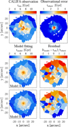Fig. 8

Binned age map and best-fitting models for NGC 0171. Top panels: binned age map t_obs and binned error map t_obserr. Middle panels: best-fitting age map t_model and standardised residuals between mock observations and model fittings t_stdres = (t_model − t_obs)/t_obserr derived from model A. Bottom: similar to middle panels, but derived from model B.

4.4 Intrinsic stellar age distributions

Now we had the stellar orbit distributions with the stellar ages tagged to the orbits for all the 82 spiral galaxies. For each galaxy, we took all stellar orbits within the effective radius R_e and divided them into 15 bins of circularity. Then we calculated the probability density of orbits and luminosity-weighted mean stellar ages in each bin. We thus obtained the probability density distributions of orbits P(λ_z) and the intrinsic distributions of stellar ages t(λ_z) for each galaxy. We also calculated the average circularity of all stellar orbits for each galaxy. The probability density of the orbits is the same as presented in Zhu et al. (2018b), and the total orbit weight within R_e for each galaxy was normalised to unity.

We present P(λ_z) and t(λ_z) for all the 82 CALIFA spiral galaxies in Fig. 9, with the galaxies sorted by increasing stellar mass from left to right. The top panel shows the stellar orbit distributions P(λ_z), and the bottom panel shows the intrinsic stellar age distributions t(λ_z) derived from model B. The stars on all orbits become systematically older with increasing stellar mass, with a more significant increase for stars on random-motion dominated orbits than those on rotation-dominated orbits. For low-mass galaxies, stars on all orbits are similarly young. For high-mass galaxies, stars on random-motion dominated orbits become significantly older in most cases, while the ages of stars on rotation-dominated orbits span a wide range, which means that disks are much older in some cases and are young in other cases.

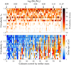Fig. 9

Probability density distributions of stellar orbits and the distributions of stellar ages within R_e vs. circularity λ_z for each of the 82 CALIFA spirals. Each column in the top panel shows the orbit probability P(λ_z) of a certain circularity bin (y-axis) for a galaxy (x-axis), as indicated by the colour bar. The sequence of galaxies along the x-axis is sorted by increasing stellar mass from left to right, with the positions of some typical stellar mass log(M_*/ M_⊙) shown at the top of the figure. For each galaxy, the average circularity of all stellar orbits is calculated, with the black folded line denoting its variation with stellar mass. The results in the top panel originally come from Fig. 2 of Zhu et al. (2018b), which plots a similar orbit distribution for each of 300 CALIFA galaxies. The bottom panel correspondingly presents the age t of each circularity bin for each galaxy, with bluer pixels indicating younger stellar populations and redder pixels denoting older populations. The horizontal dashed lines in the top and middle panels divide the cold (λ_z ≥ 0.8), warm (0.25 < λ_z < 0.8), and hot (λ_z < 0.25, including the counter-rotating orbits) components.

4.5 Stellar ages of different dynamical components

For each galaxy, we divided the orbits within R_e into three components: cold (λ_z ≥ 0.8), warm (0.25 < λ_z < 0.8), and hot (λ_z ≤ 0.25), as indicated in Fig. 9. We then calculated the luminosity-weighted orbit fraction and mean stellar age of each component. According to the morphological analysis of different orbit components (Zhu et al. 2018a), these galaxies do not have obvious counter-rotating disks, and the counter-rotating orbits usually exist in the inner parts of galaxies. Both hot and counter-rotating orbits contribute to the bulges in these galaxies, and the cold orbits make up the majority of the disks, while the warm orbits contribute either to bulges or disks. We thus took the cold component as the dynamical disk and the hot component, which includes both hot and counter-rotating orbits, as the dynamical bulge in this paper.

We divided our sample of 82 galaxies into six mass bins, with intervals defined by log(M_*/M_⊙) = 8.9, 10.0, 10.3, 10.6, 10.8, 11.0, and 11.3. For each mass bin, we calculated the average fractions of the cold, warm, and hot components, and we present them in the top panel of Fig. 10. The cold-orbit fraction peaks in galaxies with intermediate mass (M_* = 10¹⁰ ~ 10¹¹ M_⊙), and decreases at both the low-mass (M_* < 10¹⁰ M_⊙) and high-mass (M_* > 10¹¹ M_⊙) ends, while the hot-orbit fraction correspondingly increases at the low- and high-mass ends. In the bottom panel of Fig. 10, we present the average stellar ages of the cold, warm, and hot components ( $\bar{t_{cold}}$ $\overline {{t_{{\rm{cold }}}}}$ , $\bar{t_{warm}}$ $\overline {{t_{{\rm{warm }}}}}$ , and $\bar{t_{hot}}$ $\overline {{t_{{\rm{hot}}}}}$ ) in each bin. The overall uncertainties are also shown in the panel, which includes statistical uncertainties and systematic biases. For a bin with N galaxies, the statistical uncertainty contributes $σ_{stat} / \sqrt{N}$ ${\sigma _{{\rm{stat }}}}/\sqrt N$ to the upper and lower overall uncertainties, while the systematic bias $\bar{𝒟}$ $\overline D$ is added to the upper or lower overall uncertainties, depending on its sign. For example, if $\bar{𝒟} < 0$ $\overline D 0$ , the model underestimates the value, so that the upper overall uncertainty is increased by $| \bar{𝒟} |$ $|\overline D |$ to recover the true value. According to our tests in Sect. 3.4, the statistical uncertainties of each galaxy for the ages of the cold, warm, and hot components are σ_stat = 11 %, 3%, and 8%, respectively, and the corresponding systematic biases are $\bar{𝒟} = 14 %$ $\overline D = 14\%$ , −9%, and −3%. For the 66 galaxies whose inner parts of the age maps are 0.5 Gyr older than the outer parts (see Sect. 4.3), we treated them as similar to the mock galaxies and used the test results to estimate their overall uncertainties. For the other 14 galaxies that are not similar to the mock galaxies, we set a secure statistical uncertainty of 30% for the stellar ages of each component.

From Fig. 10, we find that most galaxies have younger stars in dynamically colder components, the stars in the cold disks are the youngest, and those in the hot bulges are the oldest (t_cold < t_warm < t_hot)· All three components become older with increasing stellar mass, which is consistent with the scenario that more massive spirals tend to form both their bulges and disks earlier. Furthermore, the age of the hot component t_hot obviously increases faster than that of the cold component t_cold. At M_* < 10¹⁰ M_⊙, the mean ages of the cold, warm, and hot components derived from model B ( $\bar{t_{cold}}$ $\overline {{t_{{\rm{cold }}}}}$ , $\bar{t_{warm}}$ $\overline {{t_{{\rm{warm }}}}}$ , and $\bar{t_{hot}}$ $\overline {{t_{{\rm{hot}}}}}$ ) are ~2.2 Gyr, ~2.3 Gyr, and ~2.6 Gyr, respectively, while at M_* > 10¹¹ M_⊙, the values increase to ~4.0 Gyr, ~5.1 Gyr, and ~5.9 Gyr. For comparison, we also present the results from model A. Model A provides similar mean ages as model B, but with larger uncertainties.

In order to further investigate the age difference between dynamically hot bulges and dynamically cold disks, we plot t_hot − t_cold versus stellar mass log(M_*/M_⊙) in Fig. 11. We calculated the moving average of t_hot − t_cold, and the uncertainties of the moving average have a similar definition as those in Fig. 10. In model B, the age difference between the hot and cold components increases with stellar mass from t_hot − t_cold ~ 0.5 Gyr at the low-mass end to t_hot − t_cold ~ 2 Gyr at the high-mass end. This increase of t_hot − t_cold becomes rapid around a critical mass of M_* = 10^{10 5} M_⊙. Thus, we separated our sample into low-mass (M_* ≤ 10¹⁰⁵ M_⊙) and high-mass (M_* > 10^10.5 M_⊙) spiral galaxies. For low-mass spirals, the age difference between the cold and hot components t_hot − t_cold is usually smaller than 2 Gyr, with a mean value of $\bar{t_{hot} - t_{cold}} = {0.7}_{- 0.2}^{+ 0.6} Gyr$ $\overline {{t_{{\rm{hot }}}} - {t_{{\rm{cold }}}}} = 0.7_{ - 0.2}^{ + 0.6}{\rm{Gyr}}$ ; while for high-mass spirals, the age difference spans a wide range, with a mean value of $\bar{t_{hot} - t_{cold}} = {1.7}_{- 0.2}^{+ 0.7} Gyr$ $\overline {{t_{{\rm{hot }}}} - {t_{{\rm{cold }}}}} = 1.7_{ - 0.2}^{ + 0.7}{\rm{Gyr}}$ . The scatter of the age difference in low-mass galaxies is relatively small, with σ(t_hot − t_cold) = 0.9 Gyr, while it increases to 1.4 Gyr in high-mass galaxies.

For comparison, we also present the results from model A in Fig. 11. Model A also shows a similar trend that t_hot − t_cold increases with stellar mass, but with larger uncertainties. About 80% of galaxies (66 out of 82) in model B and 79% of galaxies (65 out of 82) in model A have bulges that are older than disks (t_hot − t_cold). Although we set strong age-circularity priors in model B, the fraction of galaxies whose bulges are older than disks is not significantly different from model A, which started from a uniform prior (see Sects. 3.3 and 4.3).

Combing Figs. 9–11, we infer the assembly histories of CALIFA spiral galaxies. Most spirals (80%) have bulges that are older on average than their disks. Low-mass spirals have relatively young bulges and disks, with bulges being slightly older. This is consistent with the scenario found in the cosmological simulation TNG50: less massive spirals, especially those with M_* ≲ 10¹⁰ M_⊙, form their bulges and disks simultaneously with continuous star formation from high to intermediate redshift, with the star formation in disks lasting longer to the present day, resulting in slightly younger disks on average (Zhang et al., in prep.). High-mass spirals have old bulges, and their disks are generally younger than their bulges, but with a wide range of stellar ages. The bulges in massive galaxies (M_* ≳ 10^{10 5} M_⊙) are likely formed in the star formation burst at high redshift (Zhang et al., in prep.), while the disks are built after the bulge formation and could be destroyed by mergers but might be rebuilt afterwards (e.g. Springel et al. 2005; Robertson et al. 2006; Hopkins et al. 2009). Thus the wide range of disk stellar ages could be caused by their different merger histories. We also note that in some galaxies, the bulges are younger than disks, which could be caused by a few processes such as environmental gas stripping in the outer regions (e.g. Schaefer et al. 2019; Owers et al. 2019; Lin et al. 2019; Ding et al. 2023) and stellar winds (e.g. Pipino et al. 2008, 2010; Zibetti et al. 2020).

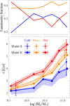Fig. 10

Luminosity-weighted orbit fractions and mean stellar ages of the cold, warm, and hot components within R_e as a function of the galaxy stellar mass. In the top panel, the blue, orange, and red lines represent the luminosity-weighted fractions of the cold, warm, and hot components in different mass bins. In the bottom panel, the coloured solid lines with dots denote the mean ages of the cold, warm, and hot components within different mass bins derived from model B. The coloured shadows represent the overall uncertainties of model B. For comparison, the mean ages of the cold, warm, and hot components derived from model A are shown by the coloured dashed lines, with the coloured error bars representing the typical overall uncertainties of model A at the low-mass and high-mass ends.

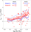Fig. 11

Age difference between the hot and cold orbit components t_hot − t_cold within R_e vs. stellar mass. The red markers indicate t_hot − t_cold derived from model B for each galaxy in our sample, with the triangles representing low-mass spirals (M_* ≤ 10¹⁰⁵M_⊙) and the circles representing high-mass spirals (M_* > 10¹⁰⁵M_⊙). The corresponding red curve represents the moving average of t_hot − t_cold. The red shadow denotes the overall uncertainties of model B. For comparison, the moving average of t_hot − t_cold and the overall uncertainties derived from model A are shown by the dashed and dotted blue lines. The horizontal dotted line means t_hot − t_cold, while the vertical dotted line denotes M_* = 10¹⁰⁵ M_⊙. The mean values of t_hot − t_cold for low-mass spirals and high-mass spirals are shown by the texts.

5 Discussion

5.1 Bulge versus disk stellar ages

Several studies in the literature have aimed to obtain the stellar ages of bulges and disks separately (e.g. Breda & Papaderos 2018; Fraser-McKelvie et al. 2018; Tabor et al. 2019; Pak et al. 2021; Johnston et al. 2022; Costantin et al. 2022; Ding et al. 2023), and we present them in this section. The bulge ages and disk ages of 135 CALIFA spiral galaxies were derived by Breda & Papaderos (2018), who used the surface photometry, the spectral modelling of IFS data based on the spectral fitting software STARLIGHT (Cid Fernandes et al. 2005), and the postprocessing tool REMOVEYOUNG (Gomes & Papaderos 2016). The stellar ages of bulges and disks were derived for 91 spiral galaxies with M_* > 10¹⁰ M_⊙ at redshift 0.14 < z ≤ 1 (Costantin et al. 2022) from the spectral energy distributions (SED) with spectral resolution R ~ 50 up to redshift z = 1 (Costantin et al. 2021), taking full advantage of the spectral information provided by SHARDS (Pérez-González et al. 2013) and the spatial resolution given by HST/CANDELS (Koekemoer et al. 2011; Grogin et al. 2011). By preforming the spectroscopic decomposition method presented in Tabor et al. (2017), the stellar ages of bulges and disks were derived for 272 MaNGA early-type galaxies (Tabor et al. 2019) and 34 CALIFA S0 galaxies (Pak et al. 2021). Based directly on photometric decomposition, 279 MaNGA S0 galaxies were decomposed, and then their bulge ages and disk ages were derived (Fraser-McKelvie et al. 2018). The bulge ages and disk ages of 78 MaNGA S0 galaxies were derived (Johnston et al. 2022) via the 2D multi-band image fitting software BUDDI (Johnston et al. 2017). Based on the same population-orbit superposition method, the stellar ages of dynamically cold disks and hot bulges were derived for 18 early-type galaxies in the Fornax Cluster by Ding et al. (2023), with the bulge and disk defined in a similar way as in our work.

In Fig. 12, we plot the bulge ages t_bulge versus the disk ages t_disk from the above works and compare them with our results. For low-mass spiral galaxies (M_* ≤ 10^{10 5} M_⊙) in CALIFA, both bulges and disks are relatively young, with bulges being ~1 Gyr older; while for high-mass spiral galaxies (M_* > 10^{10 5} M_⊙) in CALIFA, both bulges and disks become older, with bulges becoming ~2Gyr older than disks. The mass dependence of t_bulge − t_disk in our work is exactly the same as in Breda & Papaderos (2018), while their bulge ages and disk ages systematically exceed ours, which might be caused by the removal of young stellar populations in their work. The results of spiral galaxies are consistent with the works on S0 galaxies, where the bulges are slightly older (Pak et al. 2021, CALIFA) or 2–3 Gyr older on average (Fraser-McKelvie et al. 2018; Johnston et al. 2022, MaNGA) than disks. However, early-type galaxies in MaNGA have similar bulge ages and disk ages, as suggested by Tabor et al. (2019). The comparison might be biased because the definitions of bulges and disks are not exactly the same in the different methods.

The stellar ages of bulges and disks in Ding et al. (2023) were obtained using the same method as we used here, but for early-type galaxies in the Fornax cluster. The age difference between bulges and disks was found to be related with the galaxy infall time into the cluster. The ancient infallers tend to have similar bulge ages and disk ages as a result of gas removal in the cluster environment, while the intermediate and recent infallers have ~2Gyr older bulges than disks, similar to the high-mass spirals in CALIFA.

For galaxies with slightly higher redshift, the majority of spiral galaxies (85%) also have bulges older than disks, as shown in Costantin et al. (2022), and the age difference t_bulge − t_disk increases with stellar mass, which is consistent with our results. However, both t_disk and t_bulge in their work are smaller than ours, which may have two reasons. Firstly, their galaxies are at red-shift 0.14 < z ≤ 1 and our CALIFA galaxies are at z ~ 0, which will cause both their bulges and disks to be younger than ours. Secondly, our disks are defined within R_e of the galaxies, while their disks might cover larger radii. Because we expect stars in the outer disk to be younger than those in the inner disk with inside-out growth (e.g. González Delgado et al. 2015; Goddard et al. 2017; Ma et al. 2017), the average disk age will be different with different spatial coverage. When we increase the spatial coverage of the disks from R_e to 1.5 R_e, the average disk age we obtain is ~0.2 Gyr younger.

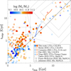Fig. 12

One-to-one comparison of bulge ages t_bulge and disk ages t_disk from different works. The dots represent 82 CALIFA spirals in our sample, with the bulge and disk ages corresponding to the ages of the hot and cold components within R_e derived from model B (t_bulge=t_hot, t_disk=t_cold). The coloured folded line illustrates the variation of mean bulge ages with mean disk ages for 135 CALIFA spiral galaxies from Breda & Papaderos (2018). The circles indicate 91 spiral galaxies at redshift 0.14 < z ≤ 1 from Costantin et al. (2022). The triangles denote 29 CALIFA S0 galaxies (shifted to 2 Gyr younger for both bulges and disks) from Pak et al. (2021). The pentacles denote 18 early-type galaxies in the Fornax Cluster from Ding et al. (2023). The stellar mass of galaxies are indicated by the colour bar. The region covered by the grey dashed lines (shifted to 4 Gyr younger for both bulges and disks) roughly shows the density distributions of 272 MaNGA early-type galaxies from Tabor et al. (2019). The grey squares and diamonds represent the mean bulge ages and disk ages in the samples of 279 MaNGA S0 galaxies (Fraser-McKelvie et al. 2018) and 78 MaNGA S0 galaxies (Johnston et al. 2022), respectively, with the corresponding error bars representing the standard deviations of bulge ages and disk ages.

5.2 Bulge stellar age versus mass

We further investigated the dependence of the bulge age t_bulge on the bulge mass log(M_b / M_⊙). We included 82 CALIFA spiral galaxies and 67 CALIFA early-type galaxies in our sample. For all CALIFA galaxies, the stellar orbit distributions were derived from the orbit-superposition method (Zhu et al. 2018b), and we defined the bulges in early-type galaxies in the same way as in spiral galaxies. The early-type galaxies show no obvious stellar age gradients, which indicates that the stellar ages of bulges and disks are statistically similar. We thus take the luminosity-weighted mean ages calculated from the age maps to represent the bulge ages of these early-type galaxies. As shown in Fig. 13, the stellar ages of bulges increase with bulge mass for both spiral galaxies and early-type galaxies. At similar bulge mass (M_b ~ 10^10.5 M_⊙), bulges in early-type galaxies span a wide range of ages and are similarly old as those in spiral galaxies.

In the top and right panels of Fig. 13, we compare the marginalised distributions of the bulge mass and the bulge ages with those from Costantin et al. (2022). They found a bimodal distribution of the bulge stellar age in their sample, and defined the bulges formed at redshift z > 3 (t > 11.7 Gyr) as the first-wave bulges and the bulges formed after z < 3 as the second-wave bulges. They claimed that the first-wave bulges built up fast in the early Universe through dissipative processes, probably evolving to the well-known z ~ 2 (t ~ 10.5 Gyr) red nuggets, while the second-wave bulges form at z = 1-2 (t = 7.9– 10.5 Gyr), and both types of bulges tend to acquire their disks by z ~ 0.5 (t ~ 5.2 Gyr). The mass and age distributions in the bulges of our spiral galaxies are similar to the second-wave bulges, except that there are more low-mass bulges in oursample, which is likely caused by the selection bias, and the bulge ages of our spiral galaxies are older than the second-wave bulges, which is likely due to the reason we explained when introducing Fig. 12. However, we lack spiral galaxies with bulges corresponding to the first-wave bulges. Instead, distributions of the bulges in our early-type galaxies are similar to those of the first-wave bulges in both bulge mass and ages. This indicates that the bulges in local early-type galaxies may have the same origin as the first-wave bulges in massive spiral galaxies at higher redshift. Firstly, a spiral galaxy containing a first-wave bulge at high redshift may quench later and become a present-day early-type galaxy. Secondly, if a first-wave bulge formed in the early Universe does not acquire a disk, it could also become a present-day early-type galaxy.

When spiral and early-type galaxies are combined, the population of bulges in CALIFA galaxies is generally consistent with the bimodality distribution of bulges in spiral galaxies at higher redshift (Costantin et al. 2022).

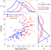Fig. 13

Bulge ages vs. bulge mass for spiral galaxies and early-type galaxies. In the main panel, the blue triangles represent 82 bulges in spiral galaxies in our sample, and their ages correspond to the ages of the hot component within R_e derived from model B. The red circles denote 67 bulges in early-type galaxies in our contrast sample, and their ages correspond to the luminosity-weighted mean ages calculated from the age maps. The solid blue line with the shadow represents the mean bulge ages and uncertainties of spiral galaxies within different mass bins, and the solid red line denotes the mean bulge ages of early-type galaxies within different mass bins. In the top and right panels, the corresponding coloured solid lines represent the marginalised distributions of bulge mass and bulge ages in our work. The dashed lines denote the distributions from Costantin et al. (2022), and the blue lines represent the second-wave bulges, and the red lines represent the first-wave bulges.

6 Summary

We adopted an innovative technique combining stellar kinematics and stellar populations, the population-orbit superposition method, to study the stellar ages of the cold, warm, and hot components for CALIFA spiral galaxies. We first evaluated the capabilities of this method on 36 mock data sets with CALIFA-like resolution created from Auriga simulated galaxies. By carefully considering the initial priors of Bayesian analysis in fitting the age maps (model B), the recovered mean ages of the cold (λ_z ≥ 0.8) and hot (λ_z ≤ 0.25) components always match the true values within 0.7 Gyr, with observational errors ranging from 5% to 20%. However, for Bayesian analysis starting from uniform priors (model A), the recovered mean ages of the cold and hot components could be biased by more than 1 Gyr, with observational errors of 15% and 20%.

We applied models A and B to 82 CALIFA spiral galaxies and obtained results consistent with each other. We took model B as the default, and our main findings are as follows:

1.
Most spirals (80%) in our sample have t_hot > t_cold, which indicates that these galaxies form their bulges first and acquire their disks later, and/or their disks experience more prolonged and extensive period of star formation;
2.
The stellar ages of the cold, warm, and hot components (t_hot, t_warm and t_cold) all increase with galaxy stellar mass. The mean ages of the cold, warm, and hot components ( $\bar{t_{hot}}$ $\overline {{t_{{\rm{hot}}}}}$ , $\bar{t_{warm}}$ $\overline {{t_{{\rm{warm}}}}}$ , and $\bar{t_{cold}}$ $\overline {{t_{{\rm{cold}}}}} \~2.2\,{\rm{Gyr}}$ ) increase from $\bar{t_{cold}} ~ 2.2 Gyr$ $\overline {{t_{{\rm{cold}}}}} \~2.3\,{\rm{Gyr}}$ , $\bar{t_{cold}} ~ 2.3 Gyr$ $\overline {{t_{{\rm{hot}}}}} \~2.6\,{\rm{Gyr}}$ , and $\bar{t_{hot}} ~ 2.6 Gyr$ $\overline {{t_{{\rm{cold}}}}} \~4.0\,{\rm{Gyr}}$ for galaxies with M_* < 10¹⁰ M_⊙ to $\bar{t_{cold}} ~ 4.0 Gyr$ $\overline {{t_{{\rm{cold}}}}} \~4.0\,{\rm{Gyr}}$ , $\bar{t_{warm}} ~ 5.1 Gyr$ $\overline {{t_{{\rm{warm}}}}} \~5.1\,{\rm{Gyr}}$ , and $\bar{t_{hot}} ~ 5.9 Gyr$ $\overline {{t_{{\rm{hot}}}}} \~5.9\,{\rm{Gyr}}$ for galaxies with M_* > 10¹¹ M_⊙;
3.
The difference in stellar ages between cold and hot components t_hot − t_cold increases with the galaxy stellar mass. The hot component is $0 {.7}_{- 0.2}^{+ 0.6} Gyr$ ${\rm{0}}{\rm{.7}}_{ - 0.2}^{ + 0.6}\,{\rm{Gyr}}$ older on average than the cold component for low-mass spirals (10^8.9 M_⊙ < M_* ≤ 10^10.5 M_⊙), while it becomes ${1.7}_{- 0.2}^{+ 0.7}$ $1.7_{ - 0.2}^{ + 0.7}$ older on average than the cold component for high-mass spirals (10^10.5 M_⊙ < M_* < 10^11.3 M_⊙).

The systematic change in stellar ages in bulges and disks from low- to high-mass galaxies indicates their different formation histories, which is generally consistent with the scenario found in the cosmologcal simulation TNG50. Low-mass spirals, especially those with M_* ≲ 10¹⁰ M_⊙, form their bulges and disks simultaneously with continuous star formation from high to intermediate redshift, with the star formations on disks lasting longer to the present day, resulting in slightly younger disks on average. The bulges in massive galaxies (M_* ≳ 10^10.5 M_⊙) are likely formed in the star formation burst at high redshift, while the disks are built after the bulge formation and could be destroyed by mergers, but are rebuilt afterwards. Various dry/wet merger histories could cause the wide range of disk ages we found in massive spiral galaxies.

Acknowledgements

The authors acknowledge the Tsinghua Astrophysics High-Performance Computing platform at Tsinghua University for providing computational and data storage resources. The research presented here is partially supported by the National Natural Science Foundation of China under grant no. Y945271001, and CAS Project for Young Scientists in Basic Research under grant no. YSBR-062. L.C. acknowledges financial support from Comunidad de Madrid under Atracción de Talento grant no. 2018-T2/TIC-11612 and from grant no. PGC2018-093499-B-I00 by the Spanish Ministry of Science and Innovation/State Agency of Research MCIN/AEI/ 10.13039/501100011033. G.v.d.V. acknowledges funding from the European Research Council (ERC) under the European Union’s Horizon 2020 research and innovation programme under grant agreement no. 724857 (Consolidator Grant ArcheoDyn).

Appendix A The surface brightness profiles and age profiles for CALIFA spiral galaxies

In Fig. A.1, we plot the r-band surface brightness profiles $\bar{μ_{r}}$ $\overline {{\mu _{\rm{r}}}}$ versus radius $\bar{R / R_{e}}$ $\overline {{R \mathord{\left/ {\vphantom {R {{R_{\rm{e}}}}}} \right. \kern-\nulldelimiterspace} {{R_{\rm{e}}}}}}$ for the cold, warm, and hot components within different mass bins, based on the results from Zhu et al. (2018b). In Fig. A.2, we present the luminosity-weighted age profiles (fobs) along the major and minor axes versus radius R/R_e, which are directly calculated based on the age maps from Zibetti et al. (2017).

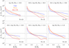Fig. A.1

Binned r-band surface brightness profiles $\bar{μ_{r}}$ $\overline {{\mu _{\rm{r}}}}$ vs radius $\bar{R / R_{e}}$ $\overline {{R \mathord{\left/ {\vphantom {R {{R_{\rm{e}}}}}} \right. \kern-\nulldelimiterspace} {{R_{\rm{e}}}}}}$ . Our sample is divided into six mass bins with intervals defined by log(M_*/ M_⊙) = 8.9,10.0, 10.3, 10.6, 10.8,11.0, and 11.3. In each panel, we bin the profiles of galaxies within a certain mass bin for cold (λ_z ≥ 0.8, blue lines), warm (0.25 < λ_z < 0.8, orange lines), and hot (λ_z ≤ 0.25, red lines) components separately. The number of galaxies N in each bin is shown by the text. The horizontal dotted lines in each panel represent the values of 10¹ and 10².

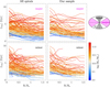Fig. A.2

Luminosity-weighted age profiles 〈t_obs〉 along the major and minor axes vs radius R/R_e. The left panels show the profiles of all 160 spiral galaxies by matching the catalogues from Zhu et al. (2018b) and Zibetti et al. (2017), while the right panels show the profiles of 82 spirals in our final sample. The ellipse on the right of the figure illustrates how we calculate the age profile: for each galaxy, we find its major axis from the image and divide the image into different regions (separated by the dotted lines) by a step of 30° starting from the major axis. Then we calculate the luminosity-weighted age profile within ±30° regions away from the major axis (magenta shadow, corresponding to the top panels) and the minor axis (grey shadow, corresponding to the bottom panels). Each fold line in the panels indicates a galaxy, with its stellar mass log(M_*/ M_⊙) indicated by the colour bar.

Appendix B A new version of age error maps and the corresponding results

Here, we define a new version of age error maps. We still binned the age map in the same way as described in Sect. 4.3, but define the age error in each bin by adapting the luminosity-weighted mean error of all pixels in that bin,

$t_{obserr}^{i} = \frac{\sum_{j = 1}^{N_{i}} L_{j} σ (t_{j})}{\sum_{j = 1}^{N_{i}} L_{j}} .$ $t_{{\rm{obserr}}}^i = {{\sum\nolimits_{j = 1}^{{N_i}} {{L_j}\sigma \left( {{t_j}} \right)} } \over {\sum\nolimits_{j = 1}^{{N_i}} {{L_j}} }}.$ (B.1)

In this way, the errors of the binned ages might be overestimated, especially in the outer regions of galaxies, in contrast to the errors defined in Eq. (13). We show this new version of the error map together with the corresponding best-fitting models for NGC 0171 in Fig. B.1. We note that we kept the results from model A unchanged as they are not influenced by the error map.

Using the new age error maps, we reran the models for all our sample galaxies with other settings unchanged and compared the recovered ages of the cold, warm, and hot components with previous results in Fig. B.2. We then replot the bottom panel of Fig. 10 by changing model A to model B with new age error maps, and present them in Fig. B.3. For different versions of error maps, the results from model B are statistically similar, which confirms the validity of our major conclusions.

Fig. B.1

Similar to Fig. 8, but using the new age error map.

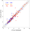Fig. B.2

One-to-one comparison of the stellar ages of the cold, warm, and hot components derived from model B under different age error maps for 82 CALIFA spirals. The x-axis represents ages calculated under the default error maps, as defined in Equation (13), while y-axis represents ages calculated under the new error maps, as defined in Equation (B.1). The blue, orange, and red circles denote cold, warm, and hot components respectively, and the corresponding colour texts show the mean difference of the ages of different components. The dashed line represent the equality of ages, while the dotted lines are ±0.5 Gyr away from the dashed line.

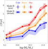Fig. B.3

Similar to the bottom panel of Fig. 10, but changing model A to model B with new age error maps.

Appendix C Data table

The main properties of 82 spiral galaxies in our sample and the corresponding modelling results are available in Table C.1.

Table C.1

The main properties of 82 spiral galaxies in our sample and the corresponding modelling results.

Notes. From left to right, they are (1) galaxy name; (2) stellar mass log(M_* /M_⊙); (3) the effective radius R_e; (4) the mean age of the cold component derived from model A; (5) the mean age of the warm component derived from model A; (6) the mean age of the hot component derived from model A; (7) the mean age of the cold component derived from model B; (8) the mean age of the warm component derived from model B; (9) the mean age of the hot component derived from model B. We refer to the journal website for the complete table.

References

Aihara, H., Allende Prieto, C., An, D., et al. 2011, ApJS, 193, 29 [NASA ADS] [CrossRef] [Google Scholar]
Bacon, R., Copin, Y., Monnet, G., et al. 2001, MNRAS, 326, 23 [Google Scholar]
Bacon, R., Conseil, S., Mary, D., et al. 2017, A & A, 608, A1 Bell, E. F., & de Jong, R. S. 2000, MNRAS, 312, 497 [Google Scholar]
Bernardi, M., Nichol, R. C., Sheth, R. K., Miller, C. J., & Brinkmann, J. 2006, AJ, 131, 1288 [NASA ADS] [CrossRef] [Google Scholar]
Bernardi, M., Domínguez Sánchez, H., Brownstein, J. R., Drory, N., & Sheth, R. K. 2019, MNRAS, 489, 5633 [Google Scholar]
Bird, J. C., Kazantzidis, S., Weinberg, D. H., et al. 2013, ApJ, 773, 43 [Google Scholar]
Bolzonella, M., Miralles, J. M., & Pelló, R. 2000, A & A, 363, 476 [NASA ADS] [Google Scholar]
Breda, I., & Papaderos, P. 2018, A & A, 614, A48 [NASA ADS] [CrossRef] [EDP Sciences] [Google Scholar]
Breda, I., Papaderos, P., & Gomes, J.-M. 2020, A & A, 640, A20 [NASA ADS] [CrossRef] [EDP Sciences] [Google Scholar]
Bryant, J. J., Owers, M. S., Robotham, A. S. G., et al. 2015, MNRAS, 447, 2857 [Google Scholar]
Bundy, K., Bershady, M. A., Law, D. R., et al. 2015, ApJ, 798, 7 [Google Scholar]
Cappellari, M. 2002, MNRAS, 333, 400 [NASA ADS] [CrossRef] [Google Scholar]
Cappellari, M. 2017, MNRAS, 466, 798 [Google Scholar]
Cappellari, M., & Copin, Y. 2003, MNRAS, 342, 345 [Google Scholar]
Cappellari, M., & Emsellem, E. 2004, PASP, 116, 138 [Google Scholar]
Cappellari, M., Emsellem, E., Krajnovic, D., et al. 2011, MNRAS, 413, 813 [NASA ADS] [CrossRef] [Google Scholar]
Cid Fernandes, R., Mateus, A., Sodré, L., Stasin´ska, G., & Gomes, J. M. 2005, MNRAS, 358, 363 [CrossRef] [Google Scholar]
Correa, C. A., Schaye, J., Clauwens, B., et al. 2017, MNRAS, 472, L45 [Google Scholar]
Costantin, L., Corsini, E. M., Méndez-Abreu, J., et al. 2018, MNRAS, 481, 3623 [CrossRef] [Google Scholar]
Costantin, L., Pérez-González, P. G., Méndez-Abreu, J., et al. 2021, ApJ, 913, 125 [NASA ADS] [CrossRef] [Google Scholar]
Costantin, L., Pérez-González, P. G., Méndez-Abreu, J., et al. 2022, ApJ, 929, 121 [NASA ADS] [CrossRef] [Google Scholar]
de Souza, R. E., Gadotti, D. A., & dos Anjos, S. 2004, ApJS, 153, 411 [NASA ADS] [CrossRef] [Google Scholar]
Ding, Y., Zhu, L., van de Ven, G., et al. 2023, A & A, 672, A84 [NASA ADS] [CrossRef] [EDP Sciences] [Google Scholar]
Du, M., Ho, L. C., Zhao, D., et al. 2019, ApJ, 884, 129 [NASA ADS] [CrossRef] [Google Scholar]
Du, M., Ho, L. C., Debattista, V. P., et al. 2020, ApJ, 895, 139 [CrossRef] [Google Scholar]
Dutton, A. A., & Macciò, A. V. 2014, MNRAS, 441, 3359 [Google Scholar]
Emsellem, E., Monnet, G., & Bacon, R. 1994, A & A, 285, 723 [NASA ADS] [Google Scholar]
Faucher-Giguère, C.-A., Lidz, A., Zaldarriaga, M., & Hernquist, L. 2009, ApJ, 703, 1416 [Google Scholar]
Fisher, D. B., & Drory, N. 2008, AJ, 136, 773 [NASA ADS] [CrossRef] [Google Scholar]
Fraser-McKelvie, A., Aragón-Salamanca, A., Merrifield, M., et al. 2018, MNRAS, 481, 5580 [Google Scholar]
Gadotti, D. A. 2009, MNRAS, 393, 1531 [Google Scholar]
Gallazzi, A., Charlot, S., Brinchmann, J., White, S. D. M., & Tremonti, C. A. 2005, MNRAS, 362, 41 [Google Scholar]
Gao, H., Ho, L. C., & Li, Z.-Y. 2022, ApJS, 262, 54 [NASA ADS] [CrossRef] [Google Scholar]
Ge, J., Mao, S., Lu, Y., Cappellari, M., & Yan, R. 2019, MNRAS, 485, 1675 [NASA ADS] [CrossRef] [Google Scholar]
Ge, J., Mao, S., Lu, Y., et al. 2021, MNRAS, 507, 2488 [NASA ADS] [CrossRef] [Google Scholar]
Gerhard, O. E. 1993, MNRAS, 265, 213 [Google Scholar]
Goddard, D., Thomas, D., Maraston, C., et al. 2017, MNRAS, 466, 4731 [NASA ADS] [Google Scholar]
Gomes, J. M., & Papaderos, P. 2016, A & A, 594, A49 [NASA ADS] [CrossRef] [EDP Sciences] [Google Scholar]
González Delgado, R. M., García-Benito, R., Pérez, E., et al. 2015, A & A, 581, A103 [CrossRef] [EDP Sciences] [Google Scholar]
Graham, A. W., & Worley, C. C. 2008, MNRAS, 388, 1708 [NASA ADS] [CrossRef] [Google Scholar]
Grand, R. J. J., Gómez, F. A., Marinacci, F., et al. 2017, MNRAS, 467, 179 [NASA ADS] [Google Scholar]
Grogin, N. A., Kocevski, D. D., Faber, S. M., et al. 2011, ApJS, 197, 35 [NASA ADS] [CrossRef] [Google Scholar]
Hopkins, P. F., Cox, T. J., Younger, J. D., & Hernquist, L. 2009, ApJ, 691, 1168 [NASA ADS] [CrossRef] [Google Scholar]
Hubble, E. P. 1926, ApJ, 64, 321 [Google Scholar]
Jin, Y., Zhu, L., Long, R. J., et al. 2019, MNRAS, 486, 4753 [Google Scholar]
Jin, Y., Zhu, L., Long, R. J., et al. 2020, MNRAS, 491, 1690 [NASA ADS] [Google Scholar]
Johnston, E. J., Aragón-Salamanca, A., Merrifield, M. R., & Bedregal, A. G. 2012, MNRAS, 422, 2590 [Google Scholar]
Johnston, E. J., Aragón-Salamanca, A., & Merrifield, M. R. 2014, MNRAS, 441, 333 [Google Scholar]
Johnston, E. J., Häußler, B., Aragón-Salamanca, A., et al. 2017, MNRAS, 465, 2317 [Google Scholar]
Johnston, E. J., Häußler, B., Jegatheesan, K., et al. 2022, MNRAS, 514, 6141 [NASA ADS] [CrossRef] [Google Scholar]
Kauffmann, G., Heckman, T. M., White, S. D. M., et al. 2003, MNRAS, 341, 54 [Google Scholar]
Kelz, A., Verheijen, M. A. W., Roth, M. M., et al. 2006, PASP, 118, 129 [Google Scholar]
Kennicutt, R. C.Jr., 1998, ARA & A, 36, 189 [NASA ADS] [CrossRef] [Google Scholar]
Koekemoer, A. M., Faber, S. M., Ferguson, H. C., et al. 2011, ApJS, 197, 36 [NASA ADS] [CrossRef] [Google Scholar]
Lawson, C. L., & Hanson, R. J. 1974, Solving least squares problems (Englewood Cliffs: Prentice-Hall) [Google Scholar]
Li, H., Mao, S., Cappellari, M., et al. 2018, MNRAS, 476, 1765 [NASA ADS] [Google Scholar]
Lin, L., Hsieh, B.-C., Pan, H.-A., et al. 2019, ApJ, 872, 50 [Google Scholar]
Ma, X., Hopkins, P. F., Wetzel, A. R., et al. 2017, MNRAS, 467, 2430 [Google Scholar]
MacArthur, L. A., Courteau, S., Bell, E., & Holtzman, J. A. 2004, ApJS, 152, 175 [NASA ADS] [CrossRef] [Google Scholar]
Marinacci, F., Pakmor, R., & Springel, V. 2014, MNRAS, 437, 1750 [Google Scholar]
McDermid, R. M., Alatalo, K., Blitz, L., et al. 2015, MNRAS, 448, 3484 [Google Scholar]
Mehlert, D., Thomas, D., Saglia, R. P., Bender, R., & Wegner, G. 2003, A & A, 407, 423 [NASA ADS] [CrossRef] [EDP Sciences] [Google Scholar]
Méndez-Abreu, J., Aguerri, J. A. L., Corsini, E. M., & Simonneau, E. 2008, A & A, 478, 353 [CrossRef] [EDP Sciences] [Google Scholar]
Méndez-Abreu, J., Ruiz-Lara, T., Sánchez-Menguiano, L., et al. 2017, A & A, 598, A32 [CrossRef] [EDP Sciences] [Google Scholar]
Méndez-Abreu, J., Sánchez, S. F., & de Lorenzo-Cáceres, A. 2019, MNRAS, 484, 4298 [Google Scholar]
Méndez-Abreu, J., de Lorenzo-Cáceres, A., & Sánchez, S. F. 2021, MNRAS, 504, 3058 [CrossRef] [Google Scholar]
Navarro, J. F., Frenk, C. S., & White, S. D. M. 1996, ApJ, 462, 563 [Google Scholar]
Neureiter, B., Thomas, J., Saglia, R., et al. 2021, MNRAS, 500, 1437 [Google Scholar]
Oh, S., Colless, M., Barsanti, S., et al. 2020, MNRAS, 495, 4638 [Google Scholar]
Owers, M. S., Hudson, M. J., Oman, K. A., et al. 2019, ApJ, 873, 52 [Google Scholar]
Pak, M., Lee, J. H., Oh, S., et al. 2021, ApJ, 921, 49 [NASA ADS] [CrossRef] [Google Scholar]
Pakmor, R., & Springel, V. 2013, MNRAS, 432, 176 [NASA ADS] [CrossRef] [Google Scholar]
Peng, C. Y., Ho, L. C., Impey, C. D., & Rix, H.-W. 2002, AJ, 124, 266 [Google Scholar]
Peng, C. Y., Ho, L. C., Impey, C. D., & Rix, H.-W. 2010, AJ, 139, 2097 [Google Scholar]
Pérez-González, P. G., Cava, A., Barro, G., et al. 2013, ApJ, 762, 46 [Google Scholar]
Pilawa, J. D., Liepold, C. M., Delgado Andrade, S. C., et al. 2022, ApJ, 928, 178 [NASA ADS] [CrossRef] [Google Scholar]
Pillepich, A., Nelson, D., Springel, V., et al. 2019, MNRAS, 490, 3196 [Google Scholar]
Pipino, A., D'Ercole, A., & Matteucci, F. 2008, A & A, 484, 679 [NASA ADS] [CrossRef] [EDP Sciences] [Google Scholar]
Pipino, A., D'Ercole, A., Chiappini, C., & Matteucci, F. 2010, MNRAS, 407, 1347 [NASA ADS] [CrossRef] [Google Scholar]
Poci, A., McDermid, R. M., Zhu, L., & van de Ven, G. 2019, MNRAS, 487, 3776 [Google Scholar]
Poci, A., McDermid, R. M., Lyubenova, M., et al. 2021, A & A, 647, A145 [NASA ADS] [CrossRef] [EDP Sciences] [Google Scholar]
Pulsoni, C., Gerhard, O., Arnaboldi, M., et al. 2020, A & A, 641, A60 [NASA ADS] [CrossRef] [EDP Sciences] [Google Scholar]
Quenneville, M. E., Liepold, C. M., & Ma, C.-P. 2021, ApJS, 254, 25 [NASA ADS] [CrossRef] [Google Scholar]
Quenneville, M. E., Liepold, C. M., & Ma, C.-P. 2022, ApJ, 926, 30 [NASA ADS] [CrossRef] [Google Scholar]
Rix, H.-W., de Zeeuw, P. T., Cretton, N., van der Marel, R. P., & Carollo, C. M. 1997, ApJ, 488, 702 [NASA ADS] [CrossRef] [Google Scholar]
Robertson, B., Bullock, J. S., Cox, T. J., et al. 2006, ApJ, 645, 986 [NASA ADS] [CrossRef] [Google Scholar]
Rodriguez-Gomez, V., Snyder, G. F., Lotz, J. M., et al. 2019, MNRAS, 483, 4140 [NASA ADS] [CrossRef] [Google Scholar]
Roth, M. M., Kelz, A., Fechner, T., et al. 2005, PASP, 117, 620 [Google Scholar]
Sánchez, S. F., Kennicutt, R. C., Gil de Paz, A., et al. 2012, A & A, 538, A8 [CrossRef] [EDP Sciences] [Google Scholar]
Sánchez, S. F., García-Benito, R., Zibetti, S., et al. 2016, A & A, 594, A36 [CrossRef] [EDP Sciences] [Google Scholar]
Santucci, G., Brough, S., van de Sande, J., et al. 2022, ApJ, 930, 153 [NASA ADS] [CrossRef] [Google Scholar]
Sarzi, M., Iodice, E., Coccato, L., et al. 2018, A & A, 616, A121 [NASA ADS] [CrossRef] [EDP Sciences] [Google Scholar]
Schaefer, A. L., Croom, S. M., Scott, N., et al. 2019, MNRAS, 483, 2851 [NASA ADS] [CrossRef] [Google Scholar]
Schaye, J., Crain, R. A., Bower, R. G., et al. 2015, MNRAS, 446, 521 [Google Scholar]
Schwarzschild, M. 1979, ApJ, 232, 236 [NASA ADS] [CrossRef] [Google Scholar]
Schwarzschild, M. 1982, ApJ, 263, 599 [NASA ADS] [CrossRef] [Google Scholar]
Schwarzschild, M. 1993, ApJ, 409, 563 [NASA ADS] [CrossRef] [Google Scholar]
Sersic, J. L. 1968, Atlas de Galaxias Australes (Cordoba, Argentina: Observatorio Astronomico) [Google Scholar]
Springel, V. 2010, MNRAS, 401, 791 [Google Scholar]
Springel, V., & Hernquist, L. 2003, MNRAS, 339, 289 [Google Scholar]
Springel, V., Di Matteo, T., & Hernquist, L. 2005, MNRAS, 361, 776 [Google Scholar]
Stinson, G. S., Bovy, J., Rix, H. W., et al. 2013, MNRAS, 436, 625 [CrossRef] [Google Scholar]
Tabor, M., Merrifield, M., Aragón-Salamanca, A., et al. 2017, MNRAS, 466, 2024 [NASA ADS] [CrossRef] [Google Scholar]
Tabor, M., Merrifield, M., Aragón-Salamanca, A., et al. 2019, MNRAS, 485, 1546 [NASA ADS] [CrossRef] [Google Scholar]
Tahmasebzadeh, B., Zhu, L., Shen, J., Gerhard, O., & Qin, Y. 2021, MNRAS, 508, 6209 [NASA ADS] [CrossRef] [Google Scholar]
Tahmasebzadeh, B., Zhu, L., Shen, J., Gerhard, O., & van de Ven, G. 2022, ApJ, 941, 109 [NASA ADS] [CrossRef] [Google Scholar]
Thater, S., Jethwa, P., Tahmasebzadeh, B., et al. 2022, A & A, 667, A51 [NASA ADS] [CrossRef] [EDP Sciences] [Google Scholar]
Thomas, D., Maraston, C., Bender, R., & Mendes de Oliveira, C. 2005, ApJ, 621, 673 [Google Scholar]
Trager, S. C., Faber, S. M., Worthey, G., & González, J. J. 2000, AJ, 119, 1645 [Google Scholar]
Trayford, J. W., Frenk, C. S., Theuns, T., Schaye, J., & Correa, C. 2019, MNRAS, 483, 744 [NASA ADS] [CrossRef] [Google Scholar]
Tsatsi, A., Macciò, A. V., van de Ven, G., & Moster, B. P. 2015, ApJ, 802, L3 [Google Scholar]
van den Bosch, R. C. E., van de Ven, G., Verolme, E. K., Cappellari, M., & de Zeeuw, P. T. 2008, MNRAS, 385, 647 [Google Scholar]
van der Marel, R. P., & Franx, M. 1993, ApJ, 407, 525 [Google Scholar]
Vasiliev, E., & Valluri, M. 2020, ApJ, 889, 39 [Google Scholar]
Verheijen, M. A. W., Bershady, M. A., Andersen, D. R., et al. 2004, Astron. Nachr., 325, 151 [Google Scholar]
Vogelsberger, M., Genel, S., Sijacki, D., et al. 2013, MNRAS, 436, 3031 [Google Scholar]
Walcher, J., Groves, B., Budavári, T., & Dale, D. 2011, Ap & SS, 331, 1 [NASA ADS] [CrossRef] [Google Scholar]
Weinzirl, T., Jogee, S., Khochfar, S., Burkert, A., & Kormendy, J. 2009, ApJ, 696, 411 [NASA ADS] [CrossRef] [Google Scholar]
Xu, D., Zhu, L., Grand, R., et al. 2019, MNRAS, 489, 842 [NASA ADS] [CrossRef] [Google Scholar]
York, D. G., Adelman, J., Anderson, John E., J., et al. 2000, AJ, 120, 1579 [NASA ADS] [CrossRef] [Google Scholar]
Zhu, L., van de Ven, G., Méndez-Abreu, J., & Obreja, A. 2018a, MNRAS, 479, 945 [Google Scholar]
Zhu, L., van de Ven, G., van den Bosch, R., et al. 2018b, Nat. Astron., 2, 233 [Google Scholar]
Zhu, L., van den Bosch, R., van de Ven, G., et al. 2018c, MNRAS, 473, 3000 [Google Scholar]
Zhu, L., van de Ven, G., Leaman, R., et al. 2020, MNRAS, 496, 1579 [Google Scholar]
Zhu, L., Pillepich, A., van de Ven, G., et al. 2022a, A & A, 660, A20 [NASA ADS] [CrossRef] [EDP Sciences] [Google Scholar]
Zhu, L., van de Ven, G., Leaman, R., et al. 2022b, A & A, 664, A115 [Google Scholar]
Zibetti, S., Gallazzi, A. R., Ascasibar, Y., et al. 2017, MNRAS, 468, 1902 [NASA ADS] [Google Scholar]
Zibetti, S., Gallazzi, A. R., Hirschmann, M., et al. 2020, MNRAS, 491, 3562 [Google Scholar]

¹ https://pypi.org/project/pymc3

All Tables

Table C.1

The main properties of 82 spiral galaxies in our sample and the corresponding modelling results.

In the text

All Figures

Fig. 1

Probability density distributions of stellar orbits P(λ_z, r) in the phase space of time-averaged radius r vs. circularity λ_z for the best-fitting model of a typical simulated spiral galaxy. The normalized probability P/P_max is indicated by the colour bar. We adopted the Voronoi-binning scheme in the λ_z-r plane to make roughly equal-weight orbit bundles. Their boundaries are represented by the blue lines.

In the text

Fig. 2

Mock surface brightness, stellar kinematic data, and best-fitting model for Au-6 with an inclination angle ϑ = 60°. From left to right: logarithmic normalised surface brightness, mean velocity V, velocity dispersion σ, skewness h₃, and kurtosis h₄. From top to bottom: mock observations, model fittings, and residuals. The residuals represent the relative deviations of the surface brightness and the standardised residuals of the kinematics.

In the text

Fig. 3

Correlation between stellar age t and circularity λ_z demonstrated with Au-6-60-5. The dotted black line represents µ_k of the uniform prior we started with, while the solid red line represents µ_k of the iteratively refined prior based on the results from the previous model run. The red dots represent the final t_k obtained in the last model iteration. Larger dot sizes indicate larger orbit weights of the orbit bundles.

In the text

Fig. 4

Parameter space of the age-circularity priors for Au-6-60-5. We use three parameters to determine the λ_z−t prior, including the age when λ_z = 0, the age when λ_z = 1, and the dispersion σ_k. The largest orange triangles denote the model with the minimum χ², and the other coloured dots represent the models within the 1σ confidence level, as indicated by the colour bar. The small black asterisks represent the models outside the 1σ confidence level.

In the text

	Fig. 5 Mock age map and best-fitting models for Au-6-60-5. Top panels: mock age map t_obs and mock error map t_obserr. Middle panels: best-fitting age map t_model and standardised residuals between mock observations and model fittings t_stdres = (t_model − t_obs)/t_obserr derived from model A. Bottom: similar to the middle panels, but derived from model B.
In the text

Fig. 6

Probability density distributions of stellar orbits P(λ_Z, t) in the phase space of circularity λ_z vs. age t for Au-6-60-5. Left panel: true distribution directly derived from the simulation. Middle panel: model-recovered distribution from model A. Right panel: model-recovered distribution from model B, which is the average of all acceptable models within the 1σ confidence level. The normalised probability P/P_max is indicated by the colour bar. The horizontal dashed lines divide the cold (λ_z ≥ 0.8), warm (0.25 < λ_z < 0.8) and hot (λ_z ≤ 0.25, including the counter-rotating orbits) components. The solid blue line in each panel represents the mean stellar age as a function of circularity from the simulations, while the dashed blue lines denote the model-recovered ages from models A and B.

In the text

Fig. 7

One-to-one comparison of the true and model-recovered age of the cold, warm, and hot orbit components for all mock data sets. Top left panel: results using model A and mock data with a MUSE-like spatial resolution from Zhu et al. (2020). Middle panels: results using model A and mock data with a CALIFA-like spatial resolution. Bottom panels: results using model B and mock data with a CALIFA-like spatial resolution. In the middle and bottom panels, the relative observational errors equal 5%, 10%, 15%, and 20% from left to right. The triangles, squares, and circles represent the mock data sets with inclination angles of 40°, 60°, and 80°. Blue, orange, and red markers denote the cold (λ_z > 0.8), warm (0.25 < λ_z < 0.8), and hot (λ_z ≤ 0.25) components. Their corresponding mean bias and statistical uncertainty are shown by the coloured texts and error bars in each panel. The dashed lines represent the equality of t_model and t_true, while the dotted lines are ±1 Gyr away from the dashed lines.

In the text

	Fig. 8 Binned age map and best-fitting models for NGC 0171. Top panels: binned age map t_obs and binned error map t_obserr. Middle panels: best-fitting age map t_model and standardised residuals between mock observations and model fittings t_stdres = (t_model − t_obs)/t_obserr derived from model A. Bottom: similar to middle panels, but derived from model B.
In the text

Fig. 9

Probability density distributions of stellar orbits and the distributions of stellar ages within R_e vs. circularity λ_z for each of the 82 CALIFA spirals. Each column in the top panel shows the orbit probability P(λ_z) of a certain circularity bin (y-axis) for a galaxy (x-axis), as indicated by the colour bar. The sequence of galaxies along the x-axis is sorted by increasing stellar mass from left to right, with the positions of some typical stellar mass log(M_*/ M_⊙) shown at the top of the figure. For each galaxy, the average circularity of all stellar orbits is calculated, with the black folded line denoting its variation with stellar mass. The results in the top panel originally come from Fig. 2 of Zhu et al. (2018b), which plots a similar orbit distribution for each of 300 CALIFA galaxies. The bottom panel correspondingly presents the age t of each circularity bin for each galaxy, with bluer pixels indicating younger stellar populations and redder pixels denoting older populations. The horizontal dashed lines in the top and middle panels divide the cold (λ_z ≥ 0.8), warm (0.25 < λ_z < 0.8), and hot (λ_z < 0.25, including the counter-rotating orbits) components.

In the text

Fig. 10

Luminosity-weighted orbit fractions and mean stellar ages of the cold, warm, and hot components within R_e as a function of the galaxy stellar mass. In the top panel, the blue, orange, and red lines represent the luminosity-weighted fractions of the cold, warm, and hot components in different mass bins. In the bottom panel, the coloured solid lines with dots denote the mean ages of the cold, warm, and hot components within different mass bins derived from model B. The coloured shadows represent the overall uncertainties of model B. For comparison, the mean ages of the cold, warm, and hot components derived from model A are shown by the coloured dashed lines, with the coloured error bars representing the typical overall uncertainties of model A at the low-mass and high-mass ends.

In the text

Fig. 11

Age difference between the hot and cold orbit components t_hot − t_cold within R_e vs. stellar mass. The red markers indicate t_hot − t_cold derived from model B for each galaxy in our sample, with the triangles representing low-mass spirals (M_* ≤ 10¹⁰⁵M_⊙) and the circles representing high-mass spirals (M_* > 10¹⁰⁵M_⊙). The corresponding red curve represents the moving average of t_hot − t_cold. The red shadow denotes the overall uncertainties of model B. For comparison, the moving average of t_hot − t_cold and the overall uncertainties derived from model A are shown by the dashed and dotted blue lines. The horizontal dotted line means t_hot − t_cold, while the vertical dotted line denotes M_* = 10¹⁰⁵ M_⊙. The mean values of t_hot − t_cold for low-mass spirals and high-mass spirals are shown by the texts.

In the text

Fig. 12

One-to-one comparison of bulge ages t_bulge and disk ages t_disk from different works. The dots represent 82 CALIFA spirals in our sample, with the bulge and disk ages corresponding to the ages of the hot and cold components within R_e derived from model B (t_bulge=t_hot, t_disk=t_cold). The coloured folded line illustrates the variation of mean bulge ages with mean disk ages for 135 CALIFA spiral galaxies from Breda & Papaderos (2018). The circles indicate 91 spiral galaxies at redshift 0.14 < z ≤ 1 from Costantin et al. (2022). The triangles denote 29 CALIFA S0 galaxies (shifted to 2 Gyr younger for both bulges and disks) from Pak et al. (2021). The pentacles denote 18 early-type galaxies in the Fornax Cluster from Ding et al. (2023). The stellar mass of galaxies are indicated by the colour bar. The region covered by the grey dashed lines (shifted to 4 Gyr younger for both bulges and disks) roughly shows the density distributions of 272 MaNGA early-type galaxies from Tabor et al. (2019). The grey squares and diamonds represent the mean bulge ages and disk ages in the samples of 279 MaNGA S0 galaxies (Fraser-McKelvie et al. 2018) and 78 MaNGA S0 galaxies (Johnston et al. 2022), respectively, with the corresponding error bars representing the standard deviations of bulge ages and disk ages.

In the text

Fig. 13

Bulge ages vs. bulge mass for spiral galaxies and early-type galaxies. In the main panel, the blue triangles represent 82 bulges in spiral galaxies in our sample, and their ages correspond to the ages of the hot component within R_e derived from model B. The red circles denote 67 bulges in early-type galaxies in our contrast sample, and their ages correspond to the luminosity-weighted mean ages calculated from the age maps. The solid blue line with the shadow represents the mean bulge ages and uncertainties of spiral galaxies within different mass bins, and the solid red line denotes the mean bulge ages of early-type galaxies within different mass bins. In the top and right panels, the corresponding coloured solid lines represent the marginalised distributions of bulge mass and bulge ages in our work. The dashed lines denote the distributions from Costantin et al. (2022), and the blue lines represent the second-wave bulges, and the red lines represent the first-wave bulges.

In the text

Fig. A.1

Binned r-band surface brightness profiles $\bar{μ_{r}}$ $\overline {{\mu _{\rm{r}}}}$ vs radius $\bar{R / R_{e}}$ $\overline {{R \mathord{\left/ {\vphantom {R {{R_{\rm{e}}}}}} \right. \kern-\nulldelimiterspace} {{R_{\rm{e}}}}}}$ . Our sample is divided into six mass bins with intervals defined by log(M_*/ M_⊙) = 8.9,10.0, 10.3, 10.6, 10.8,11.0, and 11.3. In each panel, we bin the profiles of galaxies within a certain mass bin for cold (λ_z ≥ 0.8, blue lines), warm (0.25 < λ_z < 0.8, orange lines), and hot (λ_z ≤ 0.25, red lines) components separately. The number of galaxies N in each bin is shown by the text. The horizontal dotted lines in each panel represent the values of 10¹ and 10².

In the text

Fig. A.2

Luminosity-weighted age profiles 〈t_obs〉 along the major and minor axes vs radius R/R_e. The left panels show the profiles of all 160 spiral galaxies by matching the catalogues from Zhu et al. (2018b) and Zibetti et al. (2017), while the right panels show the profiles of 82 spirals in our final sample. The ellipse on the right of the figure illustrates how we calculate the age profile: for each galaxy, we find its major axis from the image and divide the image into different regions (separated by the dotted lines) by a step of 30° starting from the major axis. Then we calculate the luminosity-weighted age profile within ±30° regions away from the major axis (magenta shadow, corresponding to the top panels) and the minor axis (grey shadow, corresponding to the bottom panels). Each fold line in the panels indicates a galaxy, with its stellar mass log(M_*/ M_⊙) indicated by the colour bar.

In the text

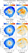	Fig. B.1 Similar to Fig. 8, but using the new age error map.
In the text

Fig. B.2

One-to-one comparison of the stellar ages of the cold, warm, and hot components derived from model B under different age error maps for 82 CALIFA spirals. The x-axis represents ages calculated under the default error maps, as defined in Equation (13), while y-axis represents ages calculated under the new error maps, as defined in Equation (B.1). The blue, orange, and red circles denote cold, warm, and hot components respectively, and the corresponding colour texts show the mean difference of the ages of different components. The dashed line represent the equality of ages, while the dotted lines are ±0.5 Gyr away from the dashed line.

In the text

	Fig. B.3 Similar to the bottom panel of Fig. 10, but changing model A to model B with new age error maps.
In the text

Current usage metrics show cumulative count of Article Views (full-text article views including HTML views, PDF and ePub downloads, according to the available data) and Abstracts Views on Vision4Press platform.

Data correspond to usage on the plateform after 2015. The current usage metrics is available 48-96 hours after online publication and is updated daily on week days.

Initial download of the metrics may take a while.

[1] Aihara, H., Allende Prieto, C., An, D., et al. 2011, ApJS, 193, 29 [NASA ADS] [CrossRef] [Google Scholar]

[2] Bacon, R., Copin, Y., Monnet, G., et al. 2001, MNRAS, 326, 23 [Google Scholar]

[3] Bacon, R., Conseil, S., Mary, D., et al. 2017, A & A, 608, A1 Bell, E. F., & de Jong, R. S. 2000, MNRAS, 312, 497 [Google Scholar]

[4] Bernardi, M., Nichol, R. C., Sheth, R. K., Miller, C. J., & Brinkmann, J. 2006, AJ, 131, 1288 [NASA ADS] [CrossRef] [Google Scholar]

[5] Bernardi, M., Domínguez Sánchez, H., Brownstein, J. R., Drory, N., & Sheth, R. K. 2019, MNRAS, 489, 5633 [Google Scholar]

[6] Bird, J. C., Kazantzidis, S., Weinberg, D. H., et al. 2013, ApJ, 773, 43 [Google Scholar]

[7] Bolzonella, M., Miralles, J. M., & Pelló, R. 2000, A & A, 363, 476 [NASA ADS] [Google Scholar]

[8] Breda, I., & Papaderos, P. 2018, A & A, 614, A48 [NASA ADS] [CrossRef] [EDP Sciences] [Google Scholar]

[9] Breda, I., Papaderos, P., & Gomes, J.-M. 2020, A & A, 640, A20 [NASA ADS] [CrossRef] [EDP Sciences] [Google Scholar]

[10] Bryant, J. J., Owers, M. S., Robotham, A. S. G., et al. 2015, MNRAS, 447, 2857 [Google Scholar]

[11] Bundy, K., Bershady, M. A., Law, D. R., et al. 2015, ApJ, 798, 7 [Google Scholar]

[12] Cappellari, M. 2002, MNRAS, 333, 400 [NASA ADS] [CrossRef] [Google Scholar]

[13] Cappellari, M. 2017, MNRAS, 466, 798 [Google Scholar]

[14] Cappellari, M., & Copin, Y. 2003, MNRAS, 342, 345 [Google Scholar]

[15] Cappellari, M., & Emsellem, E. 2004, PASP, 116, 138 [Google Scholar]

[16] Cappellari, M., Emsellem, E., Krajnovic, D., et al. 2011, MNRAS, 413, 813 [NASA ADS] [CrossRef] [Google Scholar]

[17] Cid Fernandes, R., Mateus, A., Sodré, L., Stasin´ska, G., & Gomes, J. M. 2005, MNRAS, 358, 363 [CrossRef] [Google Scholar]

[18] Correa, C. A., Schaye, J., Clauwens, B., et al. 2017, MNRAS, 472, L45 [Google Scholar]

[19] Costantin, L., Corsini, E. M., Méndez-Abreu, J., et al. 2018, MNRAS, 481, 3623 [CrossRef] [Google Scholar]

[20] Costantin, L., Pérez-González, P. G., Méndez-Abreu, J., et al. 2021, ApJ, 913, 125 [NASA ADS] [CrossRef] [Google Scholar]

[21] Costantin, L., Pérez-González, P. G., Méndez-Abreu, J., et al. 2022, ApJ, 929, 121 [NASA ADS] [CrossRef] [Google Scholar]

[22] de Souza, R. E., Gadotti, D. A., & dos Anjos, S. 2004, ApJS, 153, 411 [NASA ADS] [CrossRef] [Google Scholar]

[23] Ding, Y., Zhu, L., van de Ven, G., et al. 2023, A & A, 672, A84 [NASA ADS] [CrossRef] [EDP Sciences] [Google Scholar]

[24] Du, M., Ho, L. C., Zhao, D., et al. 2019, ApJ, 884, 129 [NASA ADS] [CrossRef] [Google Scholar]

[25] Du, M., Ho, L. C., Debattista, V. P., et al. 2020, ApJ, 895, 139 [CrossRef] [Google Scholar]

[26] Dutton, A. A., & Macciò, A. V. 2014, MNRAS, 441, 3359 [Google Scholar]

[27] Emsellem, E., Monnet, G., & Bacon, R. 1994, A & A, 285, 723 [NASA ADS] [Google Scholar]

[28] Faucher-Giguère, C.-A., Lidz, A., Zaldarriaga, M., & Hernquist, L. 2009, ApJ, 703, 1416 [Google Scholar]

[29] Fisher, D. B., & Drory, N. 2008, AJ, 136, 773 [NASA ADS] [CrossRef] [Google Scholar]

[30] Fraser-McKelvie, A., Aragón-Salamanca, A., Merrifield, M., et al. 2018, MNRAS, 481, 5580 [Google Scholar]

[31] Gadotti, D. A. 2009, MNRAS, 393, 1531 [Google Scholar]

[32] Gallazzi, A., Charlot, S., Brinchmann, J., White, S. D. M., & Tremonti, C. A. 2005, MNRAS, 362, 41 [Google Scholar]

[33] Gao, H., Ho, L. C., & Li, Z.-Y. 2022, ApJS, 262, 54 [NASA ADS] [CrossRef] [Google Scholar]

[34] Ge, J., Mao, S., Lu, Y., Cappellari, M., & Yan, R. 2019, MNRAS, 485, 1675 [NASA ADS] [CrossRef] [Google Scholar]

[35] Ge, J., Mao, S., Lu, Y., et al. 2021, MNRAS, 507, 2488 [NASA ADS] [CrossRef] [Google Scholar]

[36] Gerhard, O. E. 1993, MNRAS, 265, 213 [Google Scholar]

[37] Goddard, D., Thomas, D., Maraston, C., et al. 2017, MNRAS, 466, 4731 [NASA ADS] [Google Scholar]

[38] Gomes, J. M., & Papaderos, P. 2016, A & A, 594, A49 [NASA ADS] [CrossRef] [EDP Sciences] [Google Scholar]

[39] González Delgado, R. M., García-Benito, R., Pérez, E., et al. 2015, A & A, 581, A103 [CrossRef] [EDP Sciences] [Google Scholar]

[40] Graham, A. W., & Worley, C. C. 2008, MNRAS, 388, 1708 [NASA ADS] [CrossRef] [Google Scholar]

[41] Grand, R. J. J., Gómez, F. A., Marinacci, F., et al. 2017, MNRAS, 467, 179 [NASA ADS] [Google Scholar]

[42] Grogin, N. A., Kocevski, D. D., Faber, S. M., et al. 2011, ApJS, 197, 35 [NASA ADS] [CrossRef] [Google Scholar]

[43] Hopkins, P. F., Cox, T. J., Younger, J. D., & Hernquist, L. 2009, ApJ, 691, 1168 [NASA ADS] [CrossRef] [Google Scholar]

[44] Hubble, E. P. 1926, ApJ, 64, 321 [Google Scholar]

[45] Jin, Y., Zhu, L., Long, R. J., et al. 2019, MNRAS, 486, 4753 [Google Scholar]

[46] Jin, Y., Zhu, L., Long, R. J., et al. 2020, MNRAS, 491, 1690 [NASA ADS] [Google Scholar]

[47] Johnston, E. J., Aragón-Salamanca, A., Merrifield, M. R., & Bedregal, A. G. 2012, MNRAS, 422, 2590 [Google Scholar]

[48] Johnston, E. J., Aragón-Salamanca, A., & Merrifield, M. R. 2014, MNRAS, 441, 333 [Google Scholar]

[49] Johnston, E. J., Häußler, B., Aragón-Salamanca, A., et al. 2017, MNRAS, 465, 2317 [Google Scholar]

[50] Johnston, E. J., Häußler, B., Jegatheesan, K., et al. 2022, MNRAS, 514, 6141 [NASA ADS] [CrossRef] [Google Scholar]

[51] Kauffmann, G., Heckman, T. M., White, S. D. M., et al. 2003, MNRAS, 341, 54 [Google Scholar]

[52] Kelz, A., Verheijen, M. A. W., Roth, M. M., et al. 2006, PASP, 118, 129 [Google Scholar]

[53] Kennicutt, R. C.Jr., 1998, ARA & A, 36, 189 [NASA ADS] [CrossRef] [Google Scholar]

[54] Koekemoer, A. M., Faber, S. M., Ferguson, H. C., et al. 2011, ApJS, 197, 36 [NASA ADS] [CrossRef] [Google Scholar]

[55] Lawson, C. L., & Hanson, R. J. 1974, Solving least squares problems (Englewood Cliffs: Prentice-Hall) [Google Scholar]

[56] Li, H., Mao, S., Cappellari, M., et al. 2018, MNRAS, 476, 1765 [NASA ADS] [Google Scholar]

[57] Lin, L., Hsieh, B.-C., Pan, H.-A., et al. 2019, ApJ, 872, 50 [Google Scholar]

[58] Ma, X., Hopkins, P. F., Wetzel, A. R., et al. 2017, MNRAS, 467, 2430 [Google Scholar]

[59] MacArthur, L. A., Courteau, S., Bell, E., & Holtzman, J. A. 2004, ApJS, 152, 175 [NASA ADS] [CrossRef] [Google Scholar]

[60] Marinacci, F., Pakmor, R., & Springel, V. 2014, MNRAS, 437, 1750 [Google Scholar]

[61] McDermid, R. M., Alatalo, K., Blitz, L., et al. 2015, MNRAS, 448, 3484 [Google Scholar]

[62] Mehlert, D., Thomas, D., Saglia, R. P., Bender, R., & Wegner, G. 2003, A & A, 407, 423 [NASA ADS] [CrossRef] [EDP Sciences] [Google Scholar]

[63] Méndez-Abreu, J., Aguerri, J. A. L., Corsini, E. M., & Simonneau, E. 2008, A & A, 478, 353 [CrossRef] [EDP Sciences] [Google Scholar]

[64] Méndez-Abreu, J., Ruiz-Lara, T., Sánchez-Menguiano, L., et al. 2017, A & A, 598, A32 [CrossRef] [EDP Sciences] [Google Scholar]

[65] Méndez-Abreu, J., Sánchez, S. F., & de Lorenzo-Cáceres, A. 2019, MNRAS, 484, 4298 [Google Scholar]

[66] Méndez-Abreu, J., de Lorenzo-Cáceres, A., & Sánchez, S. F. 2021, MNRAS, 504, 3058 [CrossRef] [Google Scholar]

[67] Navarro, J. F., Frenk, C. S., & White, S. D. M. 1996, ApJ, 462, 563 [Google Scholar]

[68] Neureiter, B., Thomas, J., Saglia, R., et al. 2021, MNRAS, 500, 1437 [Google Scholar]

[69] Oh, S., Colless, M., Barsanti, S., et al. 2020, MNRAS, 495, 4638 [Google Scholar]

[70] Owers, M. S., Hudson, M. J., Oman, K. A., et al. 2019, ApJ, 873, 52 [Google Scholar]

[71] Pak, M., Lee, J. H., Oh, S., et al. 2021, ApJ, 921, 49 [NASA ADS] [CrossRef] [Google Scholar]

[72] Pakmor, R., & Springel, V. 2013, MNRAS, 432, 176 [NASA ADS] [CrossRef] [Google Scholar]

[73] Peng, C. Y., Ho, L. C., Impey, C. D., & Rix, H.-W. 2002, AJ, 124, 266 [Google Scholar]

[74] Peng, C. Y., Ho, L. C., Impey, C. D., & Rix, H.-W. 2010, AJ, 139, 2097 [Google Scholar]

[75] Pérez-González, P. G., Cava, A., Barro, G., et al. 2013, ApJ, 762, 46 [Google Scholar]

[76] Pilawa, J. D., Liepold, C. M., Delgado Andrade, S. C., et al. 2022, ApJ, 928, 178 [NASA ADS] [CrossRef] [Google Scholar]

[77] Pillepich, A., Nelson, D., Springel, V., et al. 2019, MNRAS, 490, 3196 [Google Scholar]

[78] Pipino, A., D'Ercole, A., & Matteucci, F. 2008, A & A, 484, 679 [NASA ADS] [CrossRef] [EDP Sciences] [Google Scholar]

[79] Pipino, A., D'Ercole, A., Chiappini, C., & Matteucci, F. 2010, MNRAS, 407, 1347 [NASA ADS] [CrossRef] [Google Scholar]

[80] Poci, A., McDermid, R. M., Zhu, L., & van de Ven, G. 2019, MNRAS, 487, 3776 [Google Scholar]

[81] Poci, A., McDermid, R. M., Lyubenova, M., et al. 2021, A & A, 647, A145 [NASA ADS] [CrossRef] [EDP Sciences] [Google Scholar]

[82] Pulsoni, C., Gerhard, O., Arnaboldi, M., et al. 2020, A & A, 641, A60 [NASA ADS] [CrossRef] [EDP Sciences] [Google Scholar]

[83] Quenneville, M. E., Liepold, C. M., & Ma, C.-P. 2021, ApJS, 254, 25 [NASA ADS] [CrossRef] [Google Scholar]

[84] Quenneville, M. E., Liepold, C. M., & Ma, C.-P. 2022, ApJ, 926, 30 [NASA ADS] [CrossRef] [Google Scholar]

[85] Rix, H.-W., de Zeeuw, P. T., Cretton, N., van der Marel, R. P., & Carollo, C. M. 1997, ApJ, 488, 702 [NASA ADS] [CrossRef] [Google Scholar]

[86] Robertson, B., Bullock, J. S., Cox, T. J., et al. 2006, ApJ, 645, 986 [NASA ADS] [CrossRef] [Google Scholar]

[87] Rodriguez-Gomez, V., Snyder, G. F., Lotz, J. M., et al. 2019, MNRAS, 483, 4140 [NASA ADS] [CrossRef] [Google Scholar]

[88] Roth, M. M., Kelz, A., Fechner, T., et al. 2005, PASP, 117, 620 [Google Scholar]

[89] Sánchez, S. F., Kennicutt, R. C., Gil de Paz, A., et al. 2012, A & A, 538, A8 [CrossRef] [EDP Sciences] [Google Scholar]

[90] Sánchez, S. F., García-Benito, R., Zibetti, S., et al. 2016, A & A, 594, A36 [CrossRef] [EDP Sciences] [Google Scholar]

[91] Santucci, G., Brough, S., van de Sande, J., et al. 2022, ApJ, 930, 153 [NASA ADS] [CrossRef] [Google Scholar]

[92] Sarzi, M., Iodice, E., Coccato, L., et al. 2018, A & A, 616, A121 [NASA ADS] [CrossRef] [EDP Sciences] [Google Scholar]

[93] Schaefer, A. L., Croom, S. M., Scott, N., et al. 2019, MNRAS, 483, 2851 [NASA ADS] [CrossRef] [Google Scholar]

[94] Schaye, J., Crain, R. A., Bower, R. G., et al. 2015, MNRAS, 446, 521 [Google Scholar]

[95] Schwarzschild, M. 1979, ApJ, 232, 236 [NASA ADS] [CrossRef] [Google Scholar]

[96] Schwarzschild, M. 1982, ApJ, 263, 599 [NASA ADS] [CrossRef] [Google Scholar]

[97] Schwarzschild, M. 1993, ApJ, 409, 563 [NASA ADS] [CrossRef] [Google Scholar]

[98] Sersic, J. L. 1968, Atlas de Galaxias Australes (Cordoba, Argentina: Observatorio Astronomico) [Google Scholar]

[99] Springel, V. 2010, MNRAS, 401, 791 [Google Scholar]

[100] Springel, V., & Hernquist, L. 2003, MNRAS, 339, 289 [Google Scholar]

[101] Springel, V., Di Matteo, T., & Hernquist, L. 2005, MNRAS, 361, 776 [Google Scholar]

[102] Stinson, G. S., Bovy, J., Rix, H. W., et al. 2013, MNRAS, 436, 625 [CrossRef] [Google Scholar]

[103] Tabor, M., Merrifield, M., Aragón-Salamanca, A., et al. 2017, MNRAS, 466, 2024 [NASA ADS] [CrossRef] [Google Scholar]

[104] Tabor, M., Merrifield, M., Aragón-Salamanca, A., et al. 2019, MNRAS, 485, 1546 [NASA ADS] [CrossRef] [Google Scholar]

[105] Tahmasebzadeh, B., Zhu, L., Shen, J., Gerhard, O., & Qin, Y. 2021, MNRAS, 508, 6209 [NASA ADS] [CrossRef] [Google Scholar]

[106] Tahmasebzadeh, B., Zhu, L., Shen, J., Gerhard, O., & van de Ven, G. 2022, ApJ, 941, 109 [NASA ADS] [CrossRef] [Google Scholar]

[107] Thater, S., Jethwa, P., Tahmasebzadeh, B., et al. 2022, A & A, 667, A51 [NASA ADS] [CrossRef] [EDP Sciences] [Google Scholar]

[108] Thomas, D., Maraston, C., Bender, R., & Mendes de Oliveira, C. 2005, ApJ, 621, 673 [Google Scholar]

[109] Trager, S. C., Faber, S. M., Worthey, G., & González, J. J. 2000, AJ, 119, 1645 [Google Scholar]

[110] Trayford, J. W., Frenk, C. S., Theuns, T., Schaye, J., & Correa, C. 2019, MNRAS, 483, 744 [NASA ADS] [CrossRef] [Google Scholar]

[111] Tsatsi, A., Macciò, A. V., van de Ven, G., & Moster, B. P. 2015, ApJ, 802, L3 [Google Scholar]

[112] van den Bosch, R. C. E., van de Ven, G., Verolme, E. K., Cappellari, M., & de Zeeuw, P. T. 2008, MNRAS, 385, 647 [Google Scholar]

[113] van der Marel, R. P., & Franx, M. 1993, ApJ, 407, 525 [Google Scholar]

[114] Vasiliev, E., & Valluri, M. 2020, ApJ, 889, 39 [Google Scholar]

[115] Verheijen, M. A. W., Bershady, M. A., Andersen, D. R., et al. 2004, Astron. Nachr., 325, 151 [Google Scholar]

[116] Vogelsberger, M., Genel, S., Sijacki, D., et al. 2013, MNRAS, 436, 3031 [Google Scholar]

[117] Walcher, J., Groves, B., Budavári, T., & Dale, D. 2011, Ap & SS, 331, 1 [NASA ADS] [CrossRef] [Google Scholar]

[118] Weinzirl, T., Jogee, S., Khochfar, S., Burkert, A., & Kormendy, J. 2009, ApJ, 696, 411 [NASA ADS] [CrossRef] [Google Scholar]

[119] Xu, D., Zhu, L., Grand, R., et al. 2019, MNRAS, 489, 842 [NASA ADS] [CrossRef] [Google Scholar]

[120] York, D. G., Adelman, J., Anderson, John E., J., et al. 2000, AJ, 120, 1579 [NASA ADS] [CrossRef] [Google Scholar]

[121] Zhu, L., van de Ven, G., Méndez-Abreu, J., & Obreja, A. 2018a, MNRAS, 479, 945 [Google Scholar]

[122] Zhu, L., van de Ven, G., van den Bosch, R., et al. 2018b, Nat. Astron., 2, 233 [Google Scholar]

[123] Zhu, L., van den Bosch, R., van de Ven, G., et al. 2018c, MNRAS, 473, 3000 [Google Scholar]

[124] Zhu, L., van de Ven, G., Leaman, R., et al. 2020, MNRAS, 496, 1579 [Google Scholar]

[125] Zhu, L., Pillepich, A., van de Ven, G., et al. 2022a, A & A, 660, A20 [NASA ADS] [CrossRef] [EDP Sciences] [Google Scholar]

[126] Zhu, L., van de Ven, G., Leaman, R., et al. 2022b, A & A, 664, A115 [Google Scholar]

[127] Zibetti, S., Gallazzi, A. R., Ascasibar, Y., et al. 2017, MNRAS, 468, 1902 [NASA ADS] [Google Scholar]

[128] Zibetti, S., Gallazzi, A. R., Hirschmann, M., et al. 2020, MNRAS, 491, 3562 [Google Scholar]