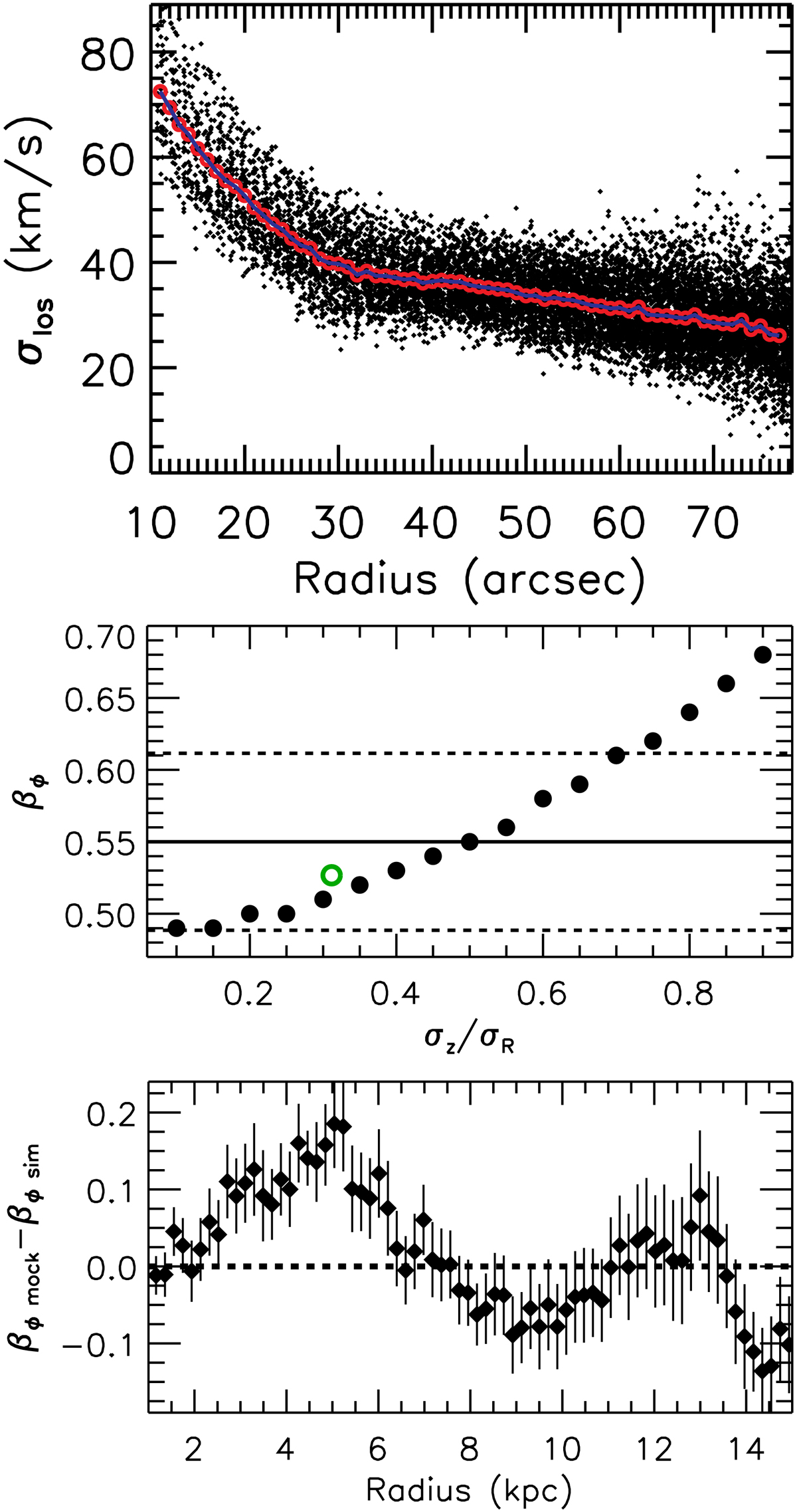
Illustrative results of the fitting of the dispersion model to the high-resolution i = 55 mock data. Top: line-of-sight velocity dispersion profile of the mock disk. Black dots indicate σ_los in each individual pixel of the so-called observed dispersion map. The red open circles correspond to the azimuthally averaged profile of that map. The blue line corresponds to the azimuthally averaged profile of the fitted model dispersion map ( = 0.4). Middle: derived anisotropy parameter as a function of the assumed value of at an example radius R = 11.5 kpc. The green open circle indicates the location of the true simulated value. The horizontal solid line and dashed lines are the median and ± 1 standard deviation of the derived values. Bottom: residual azimuthal anisotropy profile (fitted anisotropy minus true anisotropy from the simulation).