| Issue |
A&A
Volume 617, September 2018
|
|
|---|---|---|
| Article Number | A45 | |
| Number of page(s) | 23 | |
| Section | Interstellar and circumstellar matter | |
| DOI | https://doi.org/10.1051/0004-6361/201732508 | |
| Published online | 12 September 2018 | |
Anatomy of the massive star-forming region S106
The [O I] 63 μm line observed with GREAT/SOFIA as a versatile diagnostic tool for the evolution of massive stars★
1
I. Physikalisches Institut, Universität zu Köln,
Zülpicher Str. 77,
50937
Köln,
Germany
e-mail: This email address is being protected from spambots. You need JavaScript enabled to view it.
2
OASU/LAB, Université de Bordeaux,
33615
Pessac,
France
3
Max-Planck Institut für Radioastronomie,
Auf dem Hügel 69,
53121
Bonn,
Germany
4
LERMA, Obs. de Paris, ENS, PSL Research University, CNRS, Sorbonne Universités,
UPMC Univ.Paris 06,
Paris,
France
5
European Southern Observatory,
Alonso de Córdova 3107,
Vitacura,
Santiago,
Chile
6
SOFIA, USRA, NASA/Armstrong Flight Research Center,
2825 East Avenue P,
Palmdale,
CA 93550,
USA
7
DLR,
Rutherfordstraße 2,
12489
Berlin-Adlershof,
Germany
Received:
20
December
2017
Accepted:
20
May
2018
Abstract
The central area (40″ × 40″) of the bipolar nebula S106 was mapped in the [O I] line at 63.2 μm (4.74 THz) with high angular (6″) and spectral (0.24 MHz) resolution, using the GREAT heterodyne receiver on board SOFIA. The spatial and spectral emission distribution of [O I] is compared to emission in the CO 16 →15, [C II] 158 μm, and CO 11 →10 lines, mm-molecular lines, and continuum. The [O I] emission is composed of several velocity components in the range from –30 to 25 km s−1. The high-velocity blue- and red-shifted emission (v = −30 to –9 km s−1 and 8 to 25 km s−1) can be explained as arising from accelerated photodissociated gas associated with a dark lane close to the massive binary system S106 IR, and from shocks caused by the stellar wind and/or a disk–envelope interaction. At velocities from –9 to –4 km s−1 and from 0.5 to 8 km s−1 line wings are observed in most of the lines that we attribute to cooling in photodissociation regions (PDRs) created by the ionizing radiation impinging on the cavity walls. The velocity range from –4 to 0.5 km s−1 is dominated by emission from the clumpy molecular cloud, and the [O I], [C II], and high-J CO lines are excited in PDRs on clump surfaces that are illuminated by the central stars. Modelling the line emission in the different velocity ranges with the KOSMA-τ code constrains a radiation field χ of a few times 104 and densities n of a few times 104 cm−3. Considering self-absorption of the [O I] line results in higher densities (up to 106 cm−3) only for the gas component seen at high blue- and red velocities. We thus confirm the scenario found in other studies that the emission of these lines can be explained by a two-phase PDR, but attribute the high-density gas to the high-velocity component only. The dark lane has a mass of ~275 M⊙ and shows a velocity difference of ~1.4 km s−1 along its projected length of ~1 pc, determined from H13CO+ 1 →0 mapping. Its nature depends on the geometry and can be interpreted as a massive accretion flow (infall rate of ~2.5 × 10⁻⁴ M⊙ yr−1), or the remains of it, linked to S106 IR/FIR. The most likely explanation is that the binary system is at a stage of its evolution where gas accretion is counteracted by the stellar winds and radiation, leading to the very complex observed spatial and kinematic emission distribution of the various tracers.
Key words: accretion, accretion disks / ISM: atoms / ISM: molecules / ISM: clouds / HII regions / photon-dominated region (PDR)
Movie associated to Fig. 16 is available at http://www.aanda.org
© ESO 2018
1 Introduction
Massive stars form by accretion of mass in one of three ways: the core accretion model similar to low-mass stars via a prominent disk (McKee & Tan 2002), the competitive accretion scenario in a clustered environment with a very small accretion disk (Bonnell 2007; Bate 2012), or the fragmentation-induced starvation view (Peters et al. 2011) by fragmentation from gravitational instability in dense accretion flows. Only the second and third scenarios straightforwardly explain why massive stars often form in multiple systems and are found preferentially at the centre of stellar clusters (Bontemps et al. 2010). Regardless of the scenario, what is known so far about how the different stages can be observationally traced, in particular with regard to the far-infrared (FIR), can be summarized as follows (see also Tan et al. 2014):
Pre-stellar phase: massive dense clumps (masses from a few tens to a few thousands of M⊙, size ~1 pc, density n ≥ 106 cm−3, temperatureT ~ 15 K) are the locations where high-mass stars form (e.g. Beuther 2002; Motte et al. 2007; Tan et al. 2013). They often show subfragmentation into several smaller cores, i.e. pre- and protostellar objects, of size scale ≪0.1 pc (e.g. Bontemps et al. 2010), but there are also examples for isolated massive cores (e.g. Duarte-Cabral et al. 2013; Csengeri et al. 2017). Observationally, these cold dense clumps and cores are best traced by dust emission and molecular lines (such as N2 H+) in the mm and sub-mm wavelength range. In contrast, molecular line emission in the FIR is not observed in the cold dense gas phase because the energy levels of rotational transitions are too high. Only light hydrides such as CH+, CH, NH, OH, etc., can be seen in more diffuse gas. Molecular lines with lower excitation than the background continuum temperature can be observed in absorption. A good example is NH3 with its transitions from non-metastable to metastable levels, which have low excitation temperatures. For example, Wyrowski et al. (2012) successfully observed the 1.8 THz NH3 line in absorption in high-mass star-forming clumps.
Protostellar/stellar phase: massive protostars contract so quickly that there is virtually no pre-main sequence stage. Hydrogen burning starts almost instantaneously, and they are main sequence objects while still accreting. However, no well-defined Keplerian disk has been detected yet, only disk-like structures on size scales smaller than 2000 AU (e.g. Beltran et al. 2011; Sanchez-Monge et al. 2013). The envelope–disk interaction leads to an atomic jet of at least partly ionized gas orthogonal to the disk, which can then drive a molecular outflow (e.g. Kuiper et al. 2011). For low-mass protostars and massive protostars in the core accretion model, the bipolar radio jet and molecular outflow are well collimated with a time-dependent activity and opening angle (Bontemps et al. 1996). For massive protostars in the competitive accretion scenario, the jet/outflow is often poorly collimated. Surrounding lower-mass protostars can cause multiple overlapping, randomly aligned outflows so that the overall outflow pattern can be rather complex (Hunter et al. 2008). A gas distribution with a highly fragmented and filamentary structure is predicted in the fragmentation-induced starvation scenario where the dense accretion flows should be directly observable. Radiative heating leads to a higher Jeans mass so that fewer but more massive stars form (Peters et al. 2010a).
Generally, outflows from massive protostars are more massive and energetic (Beuther 2002; Duarte-Cabral et al. 2013; Maud et al. 2015) than those from low-mass protostars. Extreme UV photons (EUV, energy >13.6 eV) lead to ionization of the protostellar outflows and create an outflow-confined H II region. One class of such H II regions are those with a morphology of an hourglass shaped parsec-scale bipolar nebula such as S106. Another example is associated with the evolved star MWC349A (Gvaramadze & Menten 2012) which in addition shows a subparsec (sub-pc) nebula that is explained as being due to a biconical outflow of ionized gas pinched at the waist by a small disk seen edge-on (Cohen et al. 1985). Typical of many bipolar nebulae is also a belt of dense cold gas in the equatorial plane of the nebula (Gvaramadze et al. 2010). Though it is commonly accepted that a disk oriented perpendicular to the symmetry axis of the H II region plays a crucial role in shaping the small-scale nebula/H II region and the large-scale bipolar nebula, it is not clear how this process works in detail. In addition, the nature of the dense gas structure in the nebula waist, where the existing star or stars are embedded, is not clear. It might be the remains of an accretion flow, as was shown in numerical simulations (Peters et al. 2010a), or the result of a shock that leads to an expansion and ultimately the dispersal of the belt (Gvaramadze & Menten 2012).
The earliest stages of hyper-compact, ultra-compact, and compact H II regions are sometimes difficult to identify because the massive protostar is deeply embedded in dense gas, and even cm-emission can become optically thick. Ionized collimated jets have been seen in radio continuum for some massive protostars (e.g. Gibb et al. 2003; Guzman et al. 2014). At the stage when a larger cavity is blown out, entrained gas can also arise from the ablation of gas at the cavity borders to the surrounding molecular cloud, caused by the stellar wind. Generally, as soon as the massive star reaches the main sequence, all forms of radiative feedback (thermal heating, ionization, radiation pressure on dust) and mechanical feedback (stellar winds from the stellar surface, protostellar winds/outflows from the magneto-centrifugally driven flows powered by accretion) become important. Observationally, it is challenging to disentangle the different processes and to establish an evolutionary sequence for the protostellar phase because it is short (a few 103 yr, Duarte-Cabral et al. 2013) and because of the small number of objects to study. An additional complication is that most massive stars form as binary or multiple systems, so that the observed jet and outflow patterns are even more complex and depend on the properties of each system.
It is theobjective of this study and follow-up studies on the star-forming region S106 to identify and potentially better characterize these detailed phases by combining the spatial, velocity, and intensity information of atomic and molecular line observations and continuum from the mm to the FIR. In this first paper we focus on interpreting the [O I] 63 μm emission observed in the immediate environment of the exciting source S106 IR (see below) in the framework of a photodissociation region (PDR). A possible shock origin of the [O I] emission will be discussed and modelled in a subsequent paper, followed by a study of the large-scale structure of the bipolar nebula using [C II] 158 μm SOFIA data.
The bipolar H II region S106 in Cygnus X is an enigmatic object that has received considerable attention owing to its eye-catching appearance. Its distance was estimated to be 1.7 kpc (Schneider et al. 2007) and then determined with maser parallax measurements to be 1.3 ± 0.1 kpc (Xu et al. 2013). In the recent Gaia DR2 catalogue, the distance is derived from the trigonometric parallax to be 1.671 kpc (+738, –392 pc). In this paper, we use a value of 1.3 kpc. S106 IR was always thought to be a single late O to early B star (see Hodapp & Schneider 2008 for a summary). However, recent observations (Comerón et al. 2018) show that it is a close (separation < 0.2 AU), massive binary system, most likely consisting of a late O and a late B star, being responsible for the bipolar emission nebula (Fig. 1). Hereafter, we refer to this binary system as S106 IR. A small (only slightly larger than the beam of ~30 mas), edge-on disk-like feature around the two stars was discovered by cm-interferometry (Hoare & Muxlow 1996; Gibb & Hoare 2007), but its exact evolutionary status is not clear (Adams et al. 2015). The system already shows signatures of main sequence stars, emitting copiously in the UV (where the O star dominates) and driving an ionized wind with a velocity of 100–200 km s−1 (Simon & Fischer 1982; Bally et al. 1983) into the bipolar cavity. Associated with this system is an IR cluster withmore than 160 members (Hodapp & Rayner 1991). The centroid of the cluster lies about 30″ west and 15″ north of S106 IR and is symmetrically distributed about this location.
Figure 2 shows a cartoon of S106 with its known features and those observed to date. The two lobes of the H II region are inclined with respect to a vertical north–south axis. In addition, the northern (southern) lobe is tilted away from (towards) the observer (Solf & Carsenty 1982). A large portion of the front part of the southern cavity facing the observer has been eroded so that the backside of the cavity is visible in the optical and IR. The northern lobe is obscured byforeground gas and dust. The strongest nebular emission in the optical and near-IR arises from the shell-like structures that represent the ionization front and from the limb-brightened edges of the cavity walls. High-velocity emission of the [C II] 158 μm fine structure line and high-J CO lines (Simon et al. 2012) was interpreted as arising from swept-up material at the front and back sides of the expanding wind-driven cavity.
Another prominent feature related to S106 is a dark lane dividing the two lobes (indicated in dark blue in the cartoon) and lying apparently in front of S106 IR. It was initially interpreted as the shadow of a large-scale disk (Bally et al. 1983; Bieging 1984), but dust continuum observations (Vallée & Fiege 2005; Motte et al. 2007; Simon et al. 2012; Adams et al. 2015) revealed it to be an elongated high column-density feature associated with the extended molecular cloud (Schneider et al. 2007). Dust observations also show strong emission ≈15″ west of S106 IR, coinciding with two clusters of H2O masers (Stutzki et al. 1982; Furuya et al. 1999). The dust peak was named S106 FIR by Richer et al. (1993), and interpreted as a Class 0 young stellar object (YSO). The molecular gas close to S106 IR is highly clumped (Schneider et al. 2002) and a number of authors interpreted their observations of ionic and fine-structure lines (van den Ancker et al. 2000; Schneider et al. 2003; Simon et al. 2012; Stock et al. 2015) as arising fromphotodissociation regions (PDRs) on the surfaces of these individual clumps around S106 IR. However, most of the studies of the FIR fine-structure cooling lines of S106 were hampered because only line integrated fluxes were observed and used for PDR modelling. Here we take a different approach in that we benefit from the unprecedented velocity resolution of the German REceiver for Astronomy at Terahertz frequencies (GREAT) on board the Stratospheric Observatory for Far-Infrared Astronomy (SOFIA), and apply PDR modelling to line ratios in different velocity ranges so that we can determine more precisely the density and radiation field in individual portions of the gas.
In addition to getting a better understanding of the nature of the S106 star-forming complex itself, one of the objectives of this paper is putting our results into a larger context of how massive stars form and evolve. The paper is structured as follows. Section 2 gives observational details and Sect. 3 outlines how we realize the PDR modelling. In Sect. 4, we present maps of the observed lines and give results of PDR modelling. In Sect. 5, we develop a physical model of the S106 region and put the findings into a larger context of massive star formation. Section 6 summarizes the results of the paper.
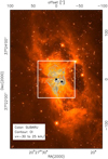 |
Fig. 1 Near-IR image (filters at J (1.25 μm), H (1.65 μm), and K′ (2.15 μm)) of S106 taken with Subaru (Oasa et al. 2006), outlining the bipolar emission nebula, with contours of velocity integrated (–30 to 25 km s−1) [O I] emission (136 to 456 K km s−1 in steps of 64 K km s−1). The area mapped with SOFIA in [O I] and CO 16 →15 emission is indicated with a white polygon. The star indicates the position of the S106 IR binary system and the triangle the position of the young stellar object (YSO) S106 FIR. |
 |
Fig. 2 Schematic view of the S106 region as seen on the sky. The nebula is tilted ≈25° to the east in the plane of the sky; the northern lobe, which is more obscured by foreground gas and dust, is inclined (≈15°) away from the observer. The southern lobe is inclined towards the observer and lacks the front side. The bipolar nebula and the H II region are embedded in an extended molecular cloud. |
2 Observations
2.1 SOFIA
The [O I] 3P1 → 3 P2 atomic fine structure line at 4.74477749 THz (63.2 μm) and the CO 16 →15 rotational line at 1.841345 THz (162.8 μm) were observed with the heterodyne receiver GREAT1 on board SOFIA during one flight on December 15, 2015, from Palmdale/California. The [O I] line was observed in the single-pixel H channel (now upgraded to a 7-pixel array), and the CO line in the single-pixel L2 channel. The average system temperatures over the total bandpass were 3641 and 5059 K for [O I] and CO, respectively. We employed a fast Fourier transform spectrometer (AFFTS). The centre intermediate frequency (IF) was 1455 MHz for the [O I] line and 1000 MHz for the CO line. The frequency resolution of the original [O I] and CO data sets is 0.244 MHz, giving a velocity resolution of ~0.04 km s−1 (16384 spectrometer channels).
Beam-switched on-the-fly maps with a scan length of 90″, a step size of 3″, and a dump time of 1 s were performed. The chopper throw was 360″ with a chop angle of 45° anti-clockwise from +RA. The map centre position refers to S106 IR (RA, Dec)(J2000) = (20h27m26s.74, 37°22′47″.9). The same area was covered three times while scanning in RA, and two times in Dec. Procedures to determine the instrument alignment and telescope efficiencies, antenna temperature and atmospheric calibration, as well as the spectrometers used, are described in Heyminck et al. (2012) and Guan et al. (2012). Tracking was done on the H-channel and the co-alignment between the H- and L2-channel is determined to be ~2″. All line intensities are reported as main beam temperatures scaled with main-beam efficiencies of 0.69 and 0.68 for[O I] and CO, respectively, and a forward efficiency of 0.97. The main beam sizes are 15.3″ for the L2 channel and 6.1″ for the H channel.
The telluric [O I] line, originating from the mesosphere, contributes as a narrow feature at the velocity of the bulk emission of the cloud (approximately +3 km s−1). We corrected for the absorption following the procedure described in Appendix A in Leurini et al. (2015), assuming that the profile can be characterized by a Gaussian. In summary, for the opacity correction the absorption strength was adjusted so as to achieve an adequate interpolation between adjacent unaffected spectral channels.
The calibrated [O I] and CO spectra were further reduced and analysed with the GILDAS software, developed and maintained by IRAM. From the spectra, a third-order baseline was removed and spectra were then averaged with 1/σ2 weighting (baseline noise). The mean r.m.s. noise temperatures per 0.6 km s−1 velocity bin are 1.9 K for [O I] (6″ beam) and 1.6 K for CO (15″ beam). We estimate that the absolute calibration uncertainty is ~20%.
For some overlays and PDR modelling, we use [C II] 158 μm and 12 CO 11 →10 data observed with SOFIA from 2012 (Simon et al. 2012) and new observations from May 2015 to December 2016 (Simon et al., in prep.).
2.2 Complementary data
2.2.1 IRAM 30 m
We use molecular line data from the IRAM2 30 m telescope, obtained in January 2016 (PI: N. Schneider). The observations were performed with two settings, one with the high-resolution spectrometer FTS50 attached to the EMIR E0 receiver (at 3 mm wavelength), and one with the lower resolution FTS200 in combination with EMIR E1 (at 1 mm wavelength). A large number of molecular lines (~20) was observed, covering a range from 85.3 to 106.1 GHz and from 89.8 to 110.5 GHz, respectively. We performed on-the-fly maps that consist of one horizontally and one vertically scanned map of size 300″ at 3 mm and 168″ at 1 mm (larger than is shown in Fig. 1). The centre position of all maps is the same as for the [O I] map. As emission-free reference position, we used a position with offset –700″, 0″ to the S106 map centre position. The quality of the data is very good, thus only baselines of first order were removed. For the H13 CO+ 1 →0 data we employ here, the average system temperature during the observations was 88 K and the average baseline rms for spectra smoothed to 15″ angular resolution and with a velocity resolution of 0.17 km s−1 is 0.16 K.
2.2.2 Other instruments
For overlaysand PDR modelling, we use published or archived continuum data from Herschel (70, 160, 250, 350, 500 μm) and FORCAST (19.7, 25.3, 31.5, 37.1 μm) (Adams et al. 2015), Spitzer (3.6, 4.5, 5.8, 8.0 μm), MAMBO (1.2 mm) (Motte et al. 2007), the VLA (Bally et al. 1983), and Subaru (Oasa et al. 2006). The flux uncertainties for the continuum data are ~10% for PACS, SPIRE, and FORCAST, and ~20% for MAMBO (see references above for these values).
3 Photodissociation region modelling
We employ the KOSMA-τ PDR model (Störzer et al. 1996; Röllig et al. 2006) to derive local physical conditions from the observed line intensities and continuum fluxes. In the following, we explain the model and our approach in more detail because this methodology will also be used for subsequent studies.
3.1 Model description
The KOSMA-τ PDR model numerically computes the energetic and chemical balance in a spherical cloud that is externally irradiated. We here use a non-clumpy model approach, i.e. a single, spherical PDR with a density gradient similar to a Bonnor–Ebert sphere, and a cloud mass of M = 100 M⊙ (the results depend only weakly on the model clump mass and we ran models with a parameter range between 10−3 and 103 M⊙). The full numerical computation scheme of KOSMA-τ involves three steps. First, the continuum radiative transfer code MCDRT (Szczerba et al. 1997) is used to compute the thermal balance of all dust components (see below) as well as the far-ultraviolet (FUV) radiative transfer within the model cloud, and the emergent continuum radiation (Röllig et al. 2013). We include a variety of different dust models, for example, the MRN model (Mathis et al. 1977) and the dust models by Weingartner & Draine (2001a). By assuming that the dust temperature is independent of the gas temperature, we then use the MCDRT output as input for the second step where the KOSMA-τ code computes the chemical and physical state of the gas. In Fig. 3, we show as an example a comparison between the observed mid-IR and FIR data at the position 3b (offsets 5″, –25″) and the best fitting dust continuum model. We determined in this way the dust continuum at all positions (nine in total) where we performed PDR modelling.
We assume a local chemical steady state, i.e. a balance between chemical formation and destruction processes of all involved species and compute their local densities and thermal equilibrium, i.e. a balance between all heating and cooling processes, resulting in local gas and dust temperatures. This is done for all radial grid positions in an iterative way to reach the numerical convergence criteria which is that the column density deviations between iterations are less than 1%. The result is the radial density and temperature profile of the model clump. In a last step the profile is used to perform the radiative transfer computations, giving the spectral line emission of the model cloud for comparison with observations (Gierens et al. 1992)3.
We use the most recent CO self-shielding functions by Visser et al. (2009) and assume a Doppler line width according to the linewidth–size relation as given by Larson (1981). The photo-electric heating is computed according to Weingartner & Draine (2001b; model 4 from their Table 2). The formation of H2 on grain surfaces follows Cazaux & Tielens (2002, 2004, 2010) and formation on polyaromatic hydrocarbon (PAH) surfaces is suppressed. For more details see Röllig et al. (2013). In addition, we use the UMIST Database for Astrochemistry chemical network (McElroy et al. 2013), including all isotopic reaction variants including 13 C and/or 18 O isotopes (Röllig & Ossenkopf 2013). In total 3766 reactions are considered and the 227 species that are included in the chemistry are listed in Table A.1. Numerically problematic reaction rate coefficients have been rescaled according to Röllig (2011). The formation of CH+ and SH+ is computed using state-to-state reaction rates (Agundez et al. 2010; Nagy et al. 2013).
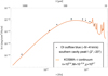 |
Fig. 3 One example (position 3a, southern cavity) for KOSMA-τ PDR model continuum emission fitting the observed continuum observations (black points) of MAMBO (1.2 mm), Herschel (PACS: 70, 160, SPIRE: 250 μm), and FORCAST (19.7, 25.3, 31.5, 37.1 μm), assuming a unity beam filling factor. The error for the flux values is generally small (see Sect. 2.2). All data were smoothed to a common angular resolution of 15″. The Herschel/SPIRE 250 μm data point has a resolution of 18″. |
3.2 Model fitting
Table 1 summarizes the model parameters. To derive local physical conditions, we compare observed line ratios4 with the corresponding model line ratios to find the best fitting model parameters. We use two line ratios, [CII]158μm∕[OI]63μm and CO(16–15)/CO(11–10), and compare them against ![Mathematical equation: $(\textrm{[CII]}_{158{\mu {\textrm{m}}}}+\textrm{[OI]}_{63{\mu {\textrm{m}}}})/\mathrm{\Sigma}_{\textrm{FIR}_{\textrm{range}}}$](/articles/aa/full_html/2018/09/aa32508-17/aa32508-17-eq1.png) . We note that we do not use here the total FIR intensity
. We note that we do not use here the total FIR intensity  , which is commonly used in PDR models (Stock et al. 2015) because we work with velocity resolved data. The parameter
  is thus only the continuum intensity in one particular velocity range. We define five velocity intervals for the [C II] and [O I] emission as explained in Sect. 4. Observationally, however, we can only determine the total FIR intensity
  obtained over all velocity ranges. For that, we derive
  by numerically integrating the continuum data between 10 and 1000 μm, stemming from FORCAST, Herschel, and MAMBO (see Sect. 2.2) using a linear interpolation. Figure 3 shows an example of this procedure. For the determination of
  we then assume that gas and dust are well mixed and that the absolute [O I] 63 μm line integrated intensity in all velocity5 ranges is higher than that of [C II] and CO (which is the case in each velocity range for each observed/analysed position, see Table 2). With these two assumptions, the fraction of [O I] line integrated intensity in one velocity range to that in the total velocity range is the same as the fraction of
  to
to  .
.
All maps are on the same angular resolution of 15″ (also the mid- and FIR continuum data), except the CO 11 →10 map, which has a resolution of ~20″, and the Herschel/SPIRE 250 μm data, which have a resolution of 18″. In the following, we thus focus on the values for density and UV field obtained from the [CII]158 μm∕[OI]63 μm ratio since beam filling factors are eliminated to the first order and because only the [O I] and [C II] lines show emission in all velocity ranges, in contrast to the CO lines that show no emission (or only marginal amounts) at the highest velocities. The model continuum intensities are provided by MCDRT; the model line intensities are computed by KOSMA-τ.
Overview of the most important model parameters.
4 Results
4.1 [O I] Spectral line map and average spectrum
Figure 4 shows the [O I] spectral line map of the region outlined in Fig. 1 on a 6″ grid, representing the original resolution of the data. The line profiles are very complex, showing several velocity components and extended wing emission, particularly in the blue range. Some of the spectral features can be explained by self-absorption (see below). Figure 5 displays the average spectrum (across the 40″ × 40″ area indicated in Fig. 1) of [O I] together with other tracers such as [C II] and molecular lines. Based upon the [O I] line profile, the emission from other tracers, and earlier studies of S106 (Schneider et al. 2002, 2003) we define and label five distinct velocity ranges to characterize the velocity distribution in S106. We note that the terms “high-velocity” and “outflow” used here are descriptive, comprising all gas dynamics (molecular and atomic) provoked by stellar feedback (radiation, wind, shocks). In the following sections, we single out the possible origin of each of the different observed features.
High-velocity blue emission (HV-blue). v = −30 to –9 km s−1, significant emission only observed in [O I] and [C II], no emission in optically thin lines.
Blue outflow emission. v = −9 to –4 km s−1, prominent emission in all optically thick lines in the form of extended wings.
Bulk emission. v = −4 to 0.5 km s−1, commonly defined velocity range for the bulk emission of the associated molecular cloud, peak emission for all observed lines, substructure in line profiles for optically thick lines, strong self-absorption features in the [O I] line.
Red outflow emission. v = 0.5–8 km s−1, broad line wings for CO lines, individual components in [C II] and [O I]. At +3 km s−1, there is aprominent dip in the [O I] line and in all other line tracers that is due to absorption6.
High-velocity red emission (HV-red). v = 8–25 km s−1, significant emission only observed in [C II] and [O I].
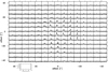 |
Fig. 4 Spectral map of [O I] emission with a velocity resolution of 1 km s−1 on a 6″ beam-sampled grid in the velocity range from –40 to 40 km s−1 and main beam brightness temperature range from –4 to 40 K. |
 |
Fig. 5 Spatially averaged spectrum of molecular and atomic lines (the spectral resolution is typically 0.2–0.6 km s−1). All spectra within the central area of 40″ × 40″ around S106 IR were included. Based upon the different spectral features, we define five major velocity ranges. The local standard of rest (lsr) velocity of the S106 molecular cloud is approximately –3 km s−1. |
4.2 Overview of [O I], [C II], and CO emission in S106
Because theline profiles of [O I] and other atomic and molecular line tracers are very complex and show a strong positional variation, we show the spectra for the positions where we performed PDR modelling in Fig. 7, an [O I] channel map (Fig. 8), and overlays of different tracers in the main velocity ranges (Appendix B). The spectra are extracted at the peak of emission in different line tracers in the respective velocity range and reflect different physical environments. They are indicated in Fig. 6 where we plot the overall line integrated [O I] emission as contours on a dust map at 19 μm (Adams et al. 2015). This overlay indicates that the total [O I] emission correlates very well with the warm dust, while the most prominent peaks of [O I] emission (positions 2, 3a, 3b) are slightly shifted with regard to the peaks of 19 μm emission. The line integrated intensities and the total FIR continuum (used for PDR modelling) are listed in Table 2. We note that positions 3a and 3b appear more than once in the table because there are peaks of emission in [O I] at different velocities.
High-velocity blue emission
The most prominent feature of the [O I] spectra is the high-velocity blue (HV-blue) emission that appears as a single component with an extended blue wing at temperatures up to 20 K at positions 1, 2, and 3c in Fig. 7. The dip in emission at –9 km s−1 is most likely not caused by self-absorption because the [C II] line has a very similar emission profile (though it cannot be excluded that both lines are affected by self-absorption). The channel map (Fig. 8) clearly shows how the HV-blue emission starts south-west of S106 IR at v = −20.6 km s−1 and then gradually develops a north-eastern component. Both peaks together are best visible at v = −12.6 km s−1.
Blue outflow emission
The channel map shows how the northern and southern cavity lobes are outlined in [O I] emission in the blue outflow velocity range (panels –8.6 to –4.6 km s−1). Position Pos. 3c represents the peak of blue outflow emission in the CO 16 →15 line, and Pos. 4 is the peak position of the blue outflow in [O I] emission in the northern cavity.
Bulk emission
Generally, the bulk emission velocity range shows a very clumpy distribution around S106 IR (panels –2.6 and –0.6 km s−1). The “hole” in the emission around S106 IR is partly caused by self-absorption, but also reflects a real lack of gas since all molecular line tracers show no emission (see Sect. 5.3). The [O I] spectra (Fig. 7) are very complex for this velocity range, showing mostly several components, which can be due to several PDR layers on clump surfaces along the line of sight and/or intrinsic self-absorption effects. Future observations of the more optically thin [O I] 145 μm line may help to decide between the different possibilities. The [O I] 145/63 μm ratio determined from velocity unresolved data (Schneider et al. 2003; Stock et al. 2015) yield a value of 0.15–0.17, indicating that one or both of the lines is optically thick. We note that the molecular cloud velocity is –1 km s−1, indicated by the 13CO 2 →1 line in (Fig. 7), while the [O I] line has a centre velocity of typically –4 km s−1. A very prominent peak of emission is found at position Pos. 3b which arises from a single clump SW of S106 IR (position S106 FIR, location of the H2 O maser), clearly visible in panel –2.6 km s−1 in the channel map. Position 5a represents the “dark lane”, which is strong in 13 CO emission and weaker in the atomic and high-J CO lines, and 5b is the NW peak of [O I] emission.
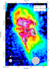 |
Fig. 6 [O I] emission of the total velocity range from –30 to 25 km s−1 in contours overlaid on a map of 19 μm emission (FORCAST; Adams et al. 2015). Positions for which we show individual spectra of various lines and report the line integrated intensities in Table 2 (in a 15″ beam) are indicated with a cross and labelled 1–6. The angular resolution of the 19 μm emissionand the [O I] beam are indicated in the panel. For comparison, the 15″ resolution we used for PDR modelling is also given. Positions 1–6 do not always correspond to peaks in [O I] emission, but also to peak emission in high- and low-J CO lines (see text for details). |
Red outflow
The velocity range from 0.5 to 8 km s−1 is strongly affected by absorption, basically all [O I] spectra show a dip between 1 and 3 km s−1 (see footnote on page 6). Significant emission is only found around v = 8 km s−1 in the southern cavity at Pos. 3a.
High-velocity red emission
The [O I] emission at velocities higher than v = 8 km s−1 is very different from the HV-blue emission; it is more diffuse and extends further away from S106 IR, mostly outlining the eastern cavity walls. Position 6 represents the [O I] peak in the northern cavity.
4.3 Shocks in S106
We did not detect the SiO (2 →1) or (5 →4) lines, classical tracers of stationary C-type (e.g. Schilke et al. 1997, Gusdorf et al. 2008a), J-type (e.g. Guillet et al. 2009), or non-stationary CJ-type (e.g. Gusdorf et al. 2008b) shocks. However, the presence of shocks that can give rise to the [O I] emission observed at high blue and red velocities and at outflow velocities cannot be excluded. These non-detections could indeed mean that the shocks are either self-irradiated (see the study of shocks with radiative precursors by Hollenbach & McKee 1989) or externally irradiated (e.g. Lesaffre et al. 2013). In the latter case, the irradiation could come from the FUV field of the central protostars. In shocks where irradiation plays a significant role, SiO is expected to be converted to Si and Si+. These species can be observed through three transitions: the 3 P1–3P0 at 129.68 μm, the 3 P2–3P1 at 68.47 μm for the Si lines, and the 2 P3∕2–2P1∕2 at 34.82 μm. The ground-state Si transitionat 129.68 μm has been marginally detected by Herschel-PACS, contrary to its excited counterpart at 68.47 μm. None of the Si lines has been detected by ISO in contrast to the Si+ transition, which was observed. The presence of atomic and ionized silicon in the gas phase, combined with the detection of optical and near-infrared lines reported by Riera et al. (1989), hints at the presence of irradiated shocks in the S106 region. Though we briefly discuss possible shocks in Sect. 5.1.1, a more sophisticated attempt to characterize their type and the role they play in the excitation of [O I] and [C II] lies out of the scope of the present study, and will be investigated in a separate publication.
5 Analysis and discussion
5.1 Emission from different velocity ranges
In this section, we qualitatively and quantitatively discuss the emission of the observed [C II], [O I], and CO lines in the different velocity intervals. Each velocity range reflects different properties of the gas in terms of radiation field, temperature, and density, and the emission can have a different origin. In particular the [O I] and high-J CO lines can originate from PDRs, i.e. UV-heated clump surfaces and cavity walls, and/or from shocks due to disk–envelope interactions (accretion shock) and local shocks when the stellar winds hit the cavity walls. One way to determine the origin of the emission is by studying its velocity structure (see Sects. 5.1.1 and 5.1.2). The excitation energies for [C II] and [O I] emission are 91 and 228 K, respectively. These transitions are easily excited by collisions with H and H2 in a PDR with different temperature layers. The critical densities for [O I] and [C II] are then 5 × 10⁵ and 3 × 103 cm−3, respectively. The high-J CO lines (16 →15 and 11 →10) have higher excitation energies, ~750 and ~365 K, and when the emission is purely thermal these lines probe hot gas associated with the PDR/molecular cloud layer at critical densities of 2 × 10⁶ and 4 × 105 cm−3, respectively. Though we discuss a possible origin from shocks in the following subsections, we use the observed FIR line ratios and the FIR flux only for PDR modelling.
The observed line intensities in the different velocity ranges and the total line integrated intensity and the fraction of intensity are listed in Table 2. All results from PDR modelling for the individual velocity ranges are summarized in Fig. 9 and Fig. 10 where we show the KOSMA-τ results for the [CII]158 μm∕[OI]63 μm and CO(16–15)/CO(11–10) line ratios as iso-contours. Dashed lines show contours of constant FUV fields, while black contours represent lines of constant density. In Tables 3 and 4, we summarize the observed ratios and give the model parameters corresponding to their position in the diagnostic Figs. 9 and 10.
Using the observed line ratios as diagnostics for PDR modelling involves several caveats which need to be kept in mind. Firstly, we use a non-clumpy PDR model because a more sophisticated set-up, as was used when studying the Orion Bar (Andree-Labsch et al. 2017), is beyond the scope of this paper. Secondly, the [O I] 63 μm line and to a lesser extent the [C II] 158 μm line are affected by self-absorption. This becomes obvious in the line profiles (Fig. 7), and is indicated by the low [O I] 145/63 μm ratio of < 0.2 (Schneider et al. 2003; Stock et al. 2015). If the [O I] 63 μm line is only moderately optically thick (τ ~ 1–2), Liseau et al. (2006) showed that self-absorption is responsible for the low ratio. We thus additionally constrained the PDR models using an [O I] intensity for all velocity ranges that is a factor 2, 4, and 10 higher. This is only a first approximation, but it allows us to estimate how the density and the radiation field change with varying [O I] line intensity. Using a much higher [O I] intensity (4 and 10 times the observed value) results in higher densities (typically 105−6 cm−3) for all positions but in a much lower radiation field (typically χ ~ 102−3). Such a low radiation field is not supported by observations; for example, we determine from Herschel flux measurements (see Sect. 5.2) a value of χ ~ (2–4) × 104 as a lower limit. We thus only use the results of a PDR model with the nominal [O I] intensity, and one that is a factor of 2 higher (given in Cols. 7 and 8 in Tables 3 and 4 in parentheses.)
 |
Fig. 8 Channel map of [O I] emission in 2 km s−1 velocity bins. The contour levels are 5, 10, 20, 45, and 60 K km s−1. The logarithmic colour scale ranges from 1.5 to 60 K km s−1. The star indicates the binary system S106 IR and the triangle S106 FIR. |
 |
Fig. 9 PDR diagnostic diagrams for observed fine-structure lines based on the KOSMA-τ PDR model for a clump of M = 100 M⊙.
|
![Mathematical equation: $[\rm CII]_{158\,{\mu {\textrm{m}}}}/[\rm OI]_{63\,{\mu {\textrm{m}}}}$](/articles/aa/full_html/2018/09/aa32508-17/aa32508-17-eq9.png)
![Mathematical equation: $([\rm CII]_{158\,{\mu {\textrm{m}}}}+[\rm OI]_{63\,{\mu {\textrm{m}}}})/\mathrm{\Sigma}_{\textrm{FIR}}$](/articles/aa/full_html/2018/09/aa32508-17/aa32508-17-eq10.png)
5.1.1 High-velocity blue and red range
The HV-blue (v < –9 km s−1) [O I] emission is spatially concentrated in two regions northeast (Pos. 1) and southwest (Pos. 2) of S106 IR (Fig. 11). Position 1 is correlated with a 19 μm dust peak, and Pos. 2 is located very close to S106 IR. It is remarkable that at Pos. 1, the [O I] emission at these high blue velocities contributes ~50% of the wholeline integrated emission at this position (see Table 2). The [O I] HV-blue emission corresponds well to the [C II] emission distribution (Fig. B.1), though the latter is more extended and outlines the cavity better. The 12 CO 2 →1 emission in this velocity range (Fig. B.1) traces the molecular outflow and the cold gas of the dark lane, but is probably more affected by beam dilution (11″ resolution with respectto 6″ for [O I]). The 12CO 16 →15 and 11 →10 lines show only very weak emission at some positions (Fig. 7).
The HV-red (v > 8 km s−1) [O I] emission is more dispersed and has two peaks along the eastern limb-brightened cavity wall, and a northern peak that is not correlated with the dust. While the overall [C II] emission in this velocity range corresponds well with [O I], the 12 CO 2 →1 line is only visible at the position of the northern clump (Fig. B.5).
There are three possible explanations for the origin of the high-velocity blue and red [O I] emission: (1) disk wind in the context of an accretion shock, (2) shocks caused by the stellar wind hitting the inside of the dark lane, or (3) classical PDR emission from the inner surface of the dark lane. Further details of each possibility are given below:
- 1.
An accretion shock can occur because S106 IR is surrounded by a disk-like structure. However, considering the distance of less than 0.2 AU between the two stars, the existence of a circumbinary disk is very unlikely; it is probably only one disk or its remains that were seen in cm-interferometry. Adopting what is known for low-mass stars (see Hartmann et al. 2016 for a review), accretion of material from the disk takes place in small-scale (sub-pc) flows along magnetic field lines (see e.g. Fig. 1 in Hartmann et al. 2016). The material has high free-fall velocities (on the order of several hundred km s−1), that then causes shocks at the stellar surface. However, the resulting shock heats the gas to very high temperatures (~106 K), which is far above the excitation of the [O I] 63 μm line. Moreover, the HV [O I] emission could originate from the disk that produces a bipolar flow or jet driven by accretion energy. The observed HV-blue [O I] emission is indeed very collimated and would fit into this scenario of an atomic jet, emanating from the disk–envelope–star system. The projected velocity (towards the observer) is vlsr ~ 25 km s−1, so that the real velocity is v = vlsr∕sin(α), where α is the inclination angle of the ionized lobes. Hippelein & Münch (1981) and Solf & Carsenty (1982) determined the angle to be around 15° so that the velocity is approximately 100 km s−1 and thus consistent with high-velocity dissociative J-type shocks (see Hollenbach 1985; Hollenbach & McKee 1989 for theory, and Nisini et al. 2015; Leurini et al. 2015 for observations). However, there are two arguments against this shock scenario on a sub-pc scale. Firstly, the HV-red [O I] emission is not collimated in the same way as the HV-blue emission (Fig. 11) which would be expected in the case of a symmetric atomic jet. Moreover, the emission is much more extended (up to several parsecs) and correlates well with the cavity walls. Secondly, the CO 16 →15 line as a typical J-type shock tracer has a very low line intensity (Table 2) in this velocity range and is only visible as an extended wing (Fig. 7).
- 2.
S106 IR consists of an OB star system that has a strong stellar wind of around 200 km s−1 (Hippelein & Münch 1981). The wind is a source of high kinetic energy and develops a shock when it expands into the ambient medium, in this case hitting the inner part of the dark lane and the molecular cloud fragments close to S106 IR. The shocked gas can then cool via the [O I] 63 μm line.
- 3.
Given the proximity of the exciting S106 IR binary system, the HV [O I] emission can be explained by PDRs on the surface of surrounding clumps and from the backside of the dark lane. From the PDR model (Sect. 3.2), we derive a density of 5–6 × 104 cm−3 and an UV field of χ ~ 7 × 10⁴ from the ratio [C II]/[O I] for S106 IR and the northern HV-blue and HV-red peak emission positions. The southern HV-red [O I] peak has a lower density of 104 cm−3 and a UV field of χ = 1.6 × 10⁴ from [C II]/[O I]. These density values increase to 2 × 106 cm−3 (while the radiation field becomes slightly lower, typically χ around a few times 104) when the [O I] intensity is increased by a factor of two. The density and radiation field obtained from the CO(16 →15)/CO(11 →10) line ratio for the HV-blue emission are lower (n = 1.5 and 2.8 × 104 cm−3 and χ = 2–4 × 10⁴) and stay below 105 for the density even if the [O I] intensity increases. Modelling the HV-red CO emission is tricky because of the low line intensities (see Table 2). For Pos. 6, we derive a density of n ~ 2 × 106 cm−3 for both original and increased [O I] intensity, but the radiation field with a value of χ = 106 is uncharacteristically high.
On first sight, it is puzzling that in the high-velocity blue range we observe strong [O I] emission but nearly no CO 16 →15 emission, even though the two lines have similar critical densities. Because CO 16 →15 has a higherexcitation temperature (750 K) than [O I] (228 K), and emits much less prominently in this velocity range, we assume that this high-velocity gas is not strongly heated and consists only of gas with high densities (>106 cm−3) at T ~ 300 K. The CO 16 →15 line is then mostly subthermally excited.
 |
Fig. 10 PDR diagnostic diagrams for observed fine-structure lines based on the KOSMA-τ PDR model for a clump of M = 100 M⊙. CO(16–15)/CO(11–10) against |
![Mathematical equation: $([\rm CII]_{158\,{\mu "\textrm{m}}}+[\rm OI]_{63\,{\mu {\textrm{m}}}})/\mathrm{\Sigma}_{\textrm{FIR}}$](/articles/aa/full_html/2018/09/aa32508-17/aa32508-17-eq11.png)
![Mathematical equation: $(\mathrm{[CII]}_{158\,{\mu {\textrm{m}}}}+\mathrm{[OI]}_{63\,{\mu {\textrm{m}}}})/\mathrm{\Sigma}_{\mathrm{\textrm{FIR}_{range}}}$](/articles/aa/full_html/2018/09/aa32508-17/aa32508-17-eq12.png)
![Mathematical equation: $(\mathrm{[CII]}_{158\,{\mu {\textrm{m}}}}+\mathrm{[OI]}_{63\,{\mu {\textrm{m}}}})/\mathrm{\Sigma}_{\mathrm{\textrm{FIR}_{range}}}$](/articles/aa/full_html/2018/09/aa32508-17/aa32508-17-eq15.png)
 |
Fig. 11 [O I] line integrated emission overlayed as contours on 19 μm emission from dust (Adams et al. 2015). The left panel shows the high-velocity blue emission and the right panel the high-velocity red emission. The dust emission ranges between 0 and 2.6 Jy pix−1, the [O I] contour lines go from 30 to 100% of maximum intensity (397 K km s−1 for HV-blue and 121 K km s−1 for HV-red). |
 |
Fig. 12 [O I] line integrated emission overlayed as contours on cm emission from the VLA (Bally et al. 1983). The left panel shows the blue outflow range and the right panel the redemission. The [O I] contour lines go from 36 to 156 in steps of 10 K km s−1 for the blue outflow and 40 to 180 in steps of 10 K km s−1 for the red outflow. The star indicates the binary system S106 IR and the triangle S106 FIR. |
5.1.2 Outflow blue and red [O I] emission
The [O I] emission in the blue and red outflow velocity range (–9 to –4 km s−1 and 0.5 to 8 km s−1, respectively) outlines precisely the cavity of the bipolar nebula, illustrated in Fig. 12, which shows [O I] contours overlaid on a cm VLA image (Bally et al. 1983), and in Fig. B.2. The cm emission delineates the H II region but avoids the dark lane. Bally et al. (1983) argue that the density in the lane is so high that all ionizing radiation is absorbed (see Sect. 5.3). Similar to the [C II] emission distribution (Simon et al. 2012), the red [O I] outflow emission is absent in the northern lobe. Both [O I] and [C II] red outflow emission thus stem mostly from swept-up gas of the cavity walls from the backside of the southern lobe (since the front side does not exist). In addition, we observe limb-brightened emission at the cavity walls and, closer to S106 IR, the [O I] emission in the blue outflow range is also correlated with the clump containing S106 FIR. What is causing the gas dynamics is not clear. The stellar wind of S106 IR can provoke shocks when it hits (mechanically) the cavity walls. However, the radiation of S106 IR ionizes the interface layer between the H II region and the molecular cloud and creates a classical PDR. A mixed scenario involving “irradiated shocks” (Lesaffre et al. 2013) and/or “moving PDRs” (Störzer & Hollenbach 1998) is also possible. From our modelling, we obtain average densities at the three cavity positions (3a,b, and 4) of 1.3–5.6 × 104 cm−3 at a rather constant radiation field of χ ~ a few 104, depending on position and ratio ([C II] and [O I] or CO). Interestingly, the values for density and radiation field do not change much if we increase the [O I] intensity. Though the [C II] line and to a lesser extent the [O I] line can also be excited by collisions with electrons, we assume that only a very small fraction of [C II] emission arises from the H II region because we detected only very weak [N II] 205 μm emission. Generally, this line arises only from the H II region, so that its detection only together with a sufficient [N II] to [C II] line ratio leads us to conclude that a significant amount of [C II] also emerges from the ionized gas phase (Heiles 1994). This is not the case for S106.
In contrast to [O I], the emission distribution of the CO 16 →15 line (Fig. 13) in this velocity range shows a strong spatial correlation with the “dark lane”, peaking at position 3c, which shows the highest values of CO 16 →15 emission (Table 2). Figure B.2 shows that the peak of emission in the low-J CO lines (12 CO and 13 CO 2 →1) is slightly shifted towards S106 IR. Because the lane appears prominently in the optical image as a dark feature and consists of cold gas (see SHARC image, Fig. 14, and overlays with the low-J CO lines, Fig. B.2), the CO 16 →15 emission can only arise from a PDR layer of warm and dense gas on the backside of the lane towards S106 IR. The rather low line velocities and small line width argue against a high-velocity shock origin of the high-J CO emission, but low-velocityshocks cannot be excluded. From PDR modelling, using the CO 16 →15/11 →10 ratio at position 3c, we derive a density of 5.6 × 104 cm−3 and a radiation field of χ = 7.4 × 10⁴. For the red outflow velocity range (0.5–8 km s−1) all lines with high excitation temperature and high critical density ([O I], [C II], CO 16 →15) show a similar emission distribution (Fig. B.4) with an extended clump south of S106 IR. This velocity range is affected by absorption so that the derived line intensities and ratios are not reliable and we do not use those for PDR modelling.
Summarizing, we interpret the emission in the outflow velocity ranges for all lines as arising from PDR surfaces of heated and UV illuminated clumps around S106 IR, of ablated gas from the cavity walls, and from a PDR surface on the backside of the dark lane.
 |
Fig. 13 Optical image from the Gran Telescopio Canaries (colour) with an overlay of CO 16 →15 line integrated emission (contour levels 18.6 to 83.8 in steps of 6.5 K km s−1) in the blue outflow velocity range (–9 to –4 km s−1). The dark lane is indicated by one black contour (3 Jy) of SHARC 350 μm emission (see Fig. 13). |
 |
Fig. 14 SHARC 350 μm emission (colour wedge in Jy) with overlays of CO 16 →15 line integrated emission (levels 14 to 47 by 3 K km s−1, grey contours) in the bulk velocity range (–4 to 0.5 km s−1). |
5.1.3 Bulk emission
The velocity range from –4 to 0.5 km s−1 is dominated by widespread but clumpy [O I] emission (see channel map, Fig. 8) in which the area around S106 IR is mostly devoid of emission (best visible in panel v= −0.6 km s−1). The most prominent clump is the western one associated with S106 FIR. Two other clumps northwest and south of S106 IR (Fig. B.3) are also clearly defined, and the overall emission distribution corresponds very well with that of [C II] in this velocity range (Fig. B.3). The peaks of emission in the low-J CO lines and CO 16 →15 emission areclose to the dark lane and at the position of S106 FIR (Figs. 14 and B.3). The CO 16 →15 peak corresponds to Pos. 5a, the NW peak of [O I] emission to Pos. 5b, and the western [O I] peak to Pos. 3b, i.e. the continuum source S106 FIR (Richer et al. 1993; Little et al. 1995), possibly a low- or high-mass Class 0 YSO. Theabsolute line intensities of [O I] and [C II] emission are high and the line fractional emission is 20–40%, indicating that these lines are the most important cooling lines for this portion of the gas. The CO 16 →15 line is less strong at these positions (incontrast to the CO 11 →10 line) and excited only in the outermost surface PDR layer of the dark lane facing S106 IR. Because the density and radiation field are not veryhigh (see below), it is a fair assumption that this line is subthermally excited.
From PDR modelling, we derive a density of 1.1 (1.6) 104 cm−3 (from the [C II]/[O I] and CO ratios, respectively), and a radiation field of χ = 1.1 (2.1) 104 for Pos. 5a, i.e. the CO 16 →15 peak at theinner working surface of the dark lane. The density and radiation field (n = 3.0 × 104 cm−3 and χ = 2.7 × 10⁴) are similar at the position of the NW [O I] peak. S106 FIR shows peak emission in hot dust, but the gas density and radiation field is not elevated, i.e. n ~ 2 × 104 cm−3 and χ ~ 2.5 × 10⁴. As for the blue and red outflow velocity range, the density and radiation field do not change significantly when the [O I] intensity is increased in the PDR model.
In summary, the [O I] emission in this velocity range seems to arise from the inner cavity walls in combination with PDR surfaces of individual clumps located within the cavity, close to S106 IR.
5.2 Comparison between SOFIA results and earlier studies
This is the first time that a spectrally resolved map of the [O I] 63 μm FIR cooling line is available for S106. A [C II] 158 μm map obtained with GREAT on SOFIA was presented by Simon et al. (2012). Other observations (not spectrally resolved) of the [C II] and [O I] lines with the Infrared Space Observatory (ISO), the Kuiper Airborne Observatory (KAO), and Herschel were reported by van den Ancker et al. (2000), Schneider et al. (2003), Stock et al. (2015), respectively. These studies, however, have a much lower angular resolution (40″ to 80″) and thus contain the different physical regimes in S106 (H II region, molecular cloud bulk emission, cavity, etc.) in one beam7. Nevertheless, all studies agree that there are different gas phases with at least two temperature regimes. Schneider et al. (2003) proposed a two-phase gas model with small (<0.2 pc) high-density (n = 3 × 10⁵ to 5 × 106 cm−3) clumps with high surface temperature (T ~ 200–500 K) embedded in lower density (n ~ 104 cm−3) gas. The radiation field in these two regimes is χ ~ 105 and χ ~ 103, respectively. Stock et al. (2015), based on their PACS and SPIRE Herschel study, support this scenario. They find a two-phase regime with a hot (T ~ 400 K) region characterized by a high radiation field (χ > 105) and high density (n > 105 cm−3), based on CO rotational temperatures, and a less dense region (n ~ 104 cm−3) with moderate UV field (χ ~ 104) and a temperature of around 300 K, dominating the emission of the atomic cooling lines. They argue that a third PDR gas phase may be present with very high temperatures/radiation field and densities to explain their excess emission in the CO rotational ladder for the highest-J CO lines (J > 20). From fitting the high-J CO lines within a PDR model, they obtain a radiation field of χ ~ 105 and densities of 108 cm−3. The assumption of such high densities is somewhat problematic as they are not observed in any other way, thus excitation by shocks can also be the reason for the strong CO emission. However, the contribution of shocks is not clear. van den Ancker et al. (2000) and Stock et al. (2015) estimate that their contribution is small, while Noel et al. (2005) attribute their H2 observations to shocks. In a subsequent paper on S106, we will apply irradiated shock models and investigate whether they reproduce our observed line intensities and ratios more closely.
In this study, we explain the observed [O I], [C II], and CO line ratios with a PDR model of a single gas phase with densities of a few 104 cm−3, exposed to a radiation field χ of a few 104. This would be consistent with the lower density PDR component that was found by Schneider et al. (2003) and Stock et al. (2015). If we consider self-absorption of the [O I] line and approximate the missing emission by doubling the [O I] intensity, we find that the HV-blue and HV-red emission has its origin in much denser gas of n ~ 106 cm−3, but with a similar radiation field8 of χ = 2–3 × 10⁴. This can correspond to the high-density gas component found by van den Ancker et al. (2000), Schneider et al. (2003), and Stock et al. (2015). Because they are velocity unresolved observations, it was not possible to attribute one gas component to a certain velocity range. Our data now point toward a possible scenario in which the FIR line emission in the outflow and bulk velocity ranges arises from PDRs at lower density (a few 104 cm−3) exposed to a radiation field of a few χ = 104, while the high-density gas component is only found at the high blue and red velocities. This finding emphasizes the importance of velocity resolved observations of [O I], [C II], and high-J CO lines.
Our findings also show that we do not need to invoke a third, very high-density gas phase (Stock et al.) nor a high-temperature two-gas phase regime (at T ~ 300 K and T ~ 700 K) as was needed to model outflow emission from low-mass protostars (Kristensen et al. 2017).
5.3 The dark lane: an accretion flow or an evaporating filamentary structure?
It was shown by dust observations in the mm-wavelength range (Vallée & Fiege 2005; Motte et al. 2007), in the mid-IR with FORCAST (Adams et al. 2015), and in the FIR with SHARC (Simon et al. 2012) at 350 μm, that the dark lane east of S106 IR is a high column-density feature (see Fig. 14 for the SHARC 350 μm map). Froma column density map derived from a SED fit to the 160–500 μm flux maps of Herschel (Schneider et al. 2016), we obtain an average column density9 of 4.5 × 1022 cm−2, a total mass of 275 M⊙, and an average density of 3 × 104 cm−3 for the lane.
Our IRAM 30 m observations of H13 CO+ 1 →0 reveal the dynamics of the dark lane more precisely than earlier 12CO and 13CO data of the region (Schneider et al. 2002). Figure 15 shows a channel map of H13 CO+ 1 →0 emission in the velocity range between –1.3 and –3.2 km s−1 overlaid on the Subaru IR image (Fig 1). The emission distribution has a close link to S106 IR. It starts as a more widespread emission around –1.3 km s−1 with two lobes of emission and develops into a single feature between –2.3 and –3.2 km s−1. The peak of emission moves gradually from a position further away northeast of S106 IR at –1.8 km s−1 to a peak close to S106 IR at –3.2 km s−1. This velocity distribution is thus consistent with two possible geometries that we illustrate in Fig. 16. Either the far end of the lane is slightly tilted away from the observer and the gas flows towards S106 IR (the accretion flow scenario, in green in Fig. 16) or the far end of lane is oriented towards the observer and the gas is streaming off the lane (the dispersal scenario, in blue in Fig. 16)10. In both scenarios, the lane is located in front of the H II region because it is clearly visible as a dark feature in front of a bright H II region (e.g. Fig. 15). While this is straightforward to understand in the dispersal scenario because the lane is inclined towards the observer, the flow scenario requires that the lane should be only slightly tilted away from the observer so that it can wrap around the equatorial plane of the hourglass-shaped H II region, but still be located in front of the ionized gas phase.
The dispersal scenario was originally proposed by Hodapp & Rayner (1991). They explain the bipolar H II region as arising from an anisotropic circumstellar wind, absorbing the ionizing radiation in the equatorial plane, and postulate that the single massive star S106 IR must be in a mass-loss evolutionary state and not in an accretion phase. However, such a scenario requires an energy transfer of the stellar wind onto the dense and cold gas deep in the dark lane. We observe in [O I] and [C II] high-velocity gas around –30 km s−1 that stems from PDRs and possibly shocks, caused by the stellar wind and radiation hitting the inner working surface of the dark lane. However, the cold gas within the dark lane occurs around the bulk emission of the cloud, from –1 to –3 km s−1, and is thus decoupled from the high-velocity gas phase.
In contrast, an accretion flow scenario11 was proposed by Bally et al. (1983) based on their VLA 5 GHz data (see Fig. 12). The area just around S106 IR shows only very weak 5 GHz radio emission, indicating the absence of ionized gas (because the 5 GHz emission is not attenuated by dust). The gas at very high densities is then able to absorb the emitted ionizing radiation. Our data show that the lane can be a flow that is illuminated by S106 IR.
Both scenarios were also proposed in Balsara et al. (2001), based upon interferometric 13 CO observations. They emphasize the importance of the magnetic field that can channel material in filamentary structures onto the highest gravitational potential well. The magnetic field was found to run parallel to the dark lane (Vallée & Fiege 2005), thus consistent with an inflow of gas. A number of recent observational studies support this dynamic scenario (e.g. Schneider et al. 2010; Kirk et al. 2013; Peretto et al. 2013; Rayner et al. 2017). Despite the higher angular resolution of their 13 CO data compared to our H13 CO+ data at 30″ resolution, it is not possible to discriminate between the two views, mostly because a low-J 13 CO line is not the best tracer for dense gas. It is also not possible to tell whether accretion is still occurring. Interferometric observations are required with a high-velocity resolution of high-density tracers such as H13 CO+, H13 CN, and in particular N2 H+ (a probe for cold dense gas). This sort of observation would enable us to study the velocity structure of the dark lane and to explore the immediate environment around S106 IR.
Assuming that we indeed observe a flow towards S106 IR, the projected length l of the flow is roughly 2.2′, corresponding to ~1 pc at a distance of 1.3 kpc. The velocity difference Δv along the flow, determined from the H13 CO+ map, is ~1.4 km s−1. We assume a random distribution of orientation angles and thus an average angle of the flow to the line of sight of 57.3° so that the lifetime t of the flow calculates as t = l/(Δvtan(57.3)). The lifetime is then approximately 1.1 × 10⁶ yr, leading to a mass input rate of 2.5 × 10⁻⁴ M⊙ yr−1 (using the Herschel determined mass of the lane). This rate is lower than that found for the massive subfilaments of the DR21 ridge (a few 10−3 M⊙ yr−1, Schneider et al. 2010), but similar to that observed for Mon R2 (a few 10−4 M⊙ yr−1; Rayner et al. 2017). We note, however, that this is a very crude approximation, and does not consider the true inclination and bending of the flow.
The flow scenario is consistent with simulations of Peters et al. (2010a,b) who modelled the collapse of rotating, massive cloud cores including radiative heating by both non-ionizing and ionizing radiation. The simulations show fragmentation from gravitational instability in the dense accretion flows in which either a single massive star is formed or several massive stars with many low-mass stars within the regions of the accretion flows. Because there is competition of mass, but not in the classical meaning of “competitive accretion” (Bonnell 2007; Bate 2012), they named this process “fragmentation-induced starvation”. The simulations (Peters et al. 2010b) also show the non-uniform expansion of H II regions with the formation of bipolar lobes, very similar to what is observed for S106. The bipolar outflow structure of the H II region visible at early time steps of their runs A (single sink) and B (multiple sinks) reflects qualitatively what is seen for S106. From what is known so far, S106 IR is a binary system (Comerón et al. 2018) and is associated with a large cluster of low-mass stars, detected in the IR (Hodapp & Rayner 1991). In addition, several dense pre-stellar cores have formed in the dark lane (S20 to S24 in Motte et al. 2007), indicating ongoing fragmentation.
In the scenario of the dark lane as an ionized accretion flow in the fragmentation-induced starvation model, the observed emission distribution of [O I], [C II], and other tracers fit very well. In particular the high-velocity blue emission is consistent with gas that moves downward perpendicularly to the accretion flow, down the steepest density gradient. This causes the very focused emission seen in various tracers (Figs. 11 and B.1). Interestingly, the very complex morphology and velocity distribution of jets and outflowing gas – as we observe it for S106 – is well reproduced in the models of Kuruwita et al. (2017). They produced simulations of the outflow pattern of close (separation < 10 AU) and wide (>10 AU) binaries and showed that the geometry and velocity of the jets and outflows are strongly modified with respect to a single star.
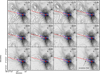 |
Fig. 15 Channel map of H13CO+ 1 →0 emission (contours in K km s−1 from 0.25 to 1.75 in steps of 0.25) obtained with the IRAM 30 m telescope. The background image is the Subaru IR image from Fig 1. The blue contour is the 3 Jy level of the SHARC 350 μm emission. The star marks the position of the binary system S106 IR; the dashed red line indicates the run of the dark lane, i.e. thepossible accretion flow. |
 |
Fig. 16 Schematic view of two possible scenarios (shown at the same time) explaining the nature of the dark lane. The front view (left panel), as S106 is seen on the sky, does not allow us to distinguish between infall scenario (dark lane in green) or expansion scenario (dark lane in blue) of the gas in the dark lane. The middle view shows best the “accretion flow” scenario, i.e. how the (green) dark lane wraps around the equatorial waist of the hourglass-nebula. The right view shows how the (blue) dark lane, which is more detached from the nebula, is tilted towards the observer and dispersed. An animated version of this cartoon is available online. |
6 Summary: a scenario for S106 IR
Summarizing our observational results and what is already known about S106, we develop the following scenario:
S106 IRis a binary system with two stars that are sources of a strong UV field and stellar wind. The very small disk-like structure that was detected in cm-interferometry can be an intact accretion disk that is connectedto a large-scale accretion flow, known as the dark lane or the remains of a disk without a link to the dark lane. The lane is illuminated by the more massive star of the system, presumably an O9 star with 20 M⊙ (the companion has a preliminary classification as a B8 star with ~3 M⊙; Comerón et al. 2018), and forms a dense hot PDR that cools mostly via [O I] 63 μm and CO 16 →15 emission. The PDR gas is highly dynamic; it flows fast and follows the steepest density gradients of the dark lane, and “escapes” the lane close to S106 IR, giving rise to the very collimated emission distribution in the [O I] lines at velocities from –30 to –9 km s−1 and 8 to 25 km s−1. We obtain a radiation field of χ = 2–7 × 10⁴ at a density of 1.5–6 × 104 cm−3 from PDR modelling. Generally, modelling the [O I] and [C II] emission is difficult because both lines show self-absorption features. By increasing the [O I] emission by a factor of 2, we obtain that the densities in the HV emission ranges increase up to 106 cm−3, which is more consistent with earlier findings (Schneider et al. 2003; Stock et al. 2015). If the emission in this velocity range could also arise from a shock (disk-envelope interaction and/or radiation and stellar wind hitting locally the dark lane) cannot yet be answered and will be addressed in an upcoming study.
The gas in the blue and red outflow velocity ranges (from –9 to –4 km s−1 and 8 to 25 km s−1) has a very similar emission distribution compared to the optical visible lobes. The [O I] (and [C II]) emission distributions at the blue and red velocities indicate that the emission mostly arises from the back side of the southern lobe and the front side of the northern lobe. The outflow gas is entrained in the wind of S106 IR and ablated by radiation (and possibly shocks) from the cavity walls. PDR modelling gives densities typically of a few 104 cm−3 at a radiation field of χ a few 104. The low value for the density indicates that the CO 16 →15 line is most likely subthermally excited.
Molecular cloud clumps and possibly fragments of what once was the larger-scale circumbinary disk around S106 IR are seen in the close environment of the star. These clumps form PDRs on their surfaces (the most prominent one is the western clump) that emit in all lines at the cloud bulk velocity around –3 km s−1. The clumps are exposed to aradiation field χ of a ~2 × 10⁴ and the density is ~2 × 104 cm−3.
S106 IR and its bipolar H II region are embedded in a larger molecular cloud that provides the gas reservoir for a possible accretion flow onto S106 IR. Mapping of the high-density tracer H13 CO+ 1 →0 revealed a velocity gradient across the dark lane that is consistent with either a flow onto S106 IR or gas streaming away, depending on the geometry of the region. Only interferometric observations can elucidate the nature of the dark lane. The flow scenario is more consistent with the fragmentation-induced starvation scenario of Peters et al. (2010a,b) than with the monolithic collapse model of McKee & Tan (2002). As yet unclear is whether shocks driven by the ionizing stellar wind that hits the accretion flow and the cavity walls can also cause the observed emission of the FIR lines. It is also not clear to what extent the [O I] 63 μm line is self-absorbed. Higher line intensities will change the [C II]/[O I] line ratios and thus modify the outcome of the PDR models. Observations of the [O I] 145 μm line, if this line is optically thin, may help to tackle this problem.
Summarizing, this study shows that the new detection of high-velocity emission in the [O I] line, and the identification of various velocity components in other FIR lines ([C II], high-J CO), which are only now possible with the (up)GREAT receiver on SOFIA, help to diagnose more precisely the physical properties of different gas phases in complex star-forming regions.
Movie
Movie for Fig. 16. Access Supplementary Material
Acknowledgements
This work was supported by the Agence National de Recherche (ANR/France) and the Deutsche Forschungsgemeinschaft (DFG/Germany) through the project ‘GENESIS’ (ANR-16-CE92-0035-01/DFG1591/2-1). N.S. acknowledges support from the BMBF, Projekt Number 50OR1714 (MOBS - MOdellierung von Beobachtungsdaten SOFIA). This work isbased on observations made with the NASA/DLR Stratospheric Observatory for Infrared Astronomy (SOFIA). SOFIA is jointly operated by the Universities Space Research Association, Inc. (USRA), under NASA contract NAS2-97001, and the Deutsches SOFIA Institut (DSI) under DLR contract 50 OK 0901 to the University of Stuttgart. This work is based on observations carried out under project number 140-15 with the IRAM 30 m telescope. IRAM is supported by INSU/CNRS (France), MPG (Germany), and IGN (Spain). N.S. acknowledges support from the Deutsche Forschungsgemeinschaft, DFG, through project number Os 177/2-1 and 177/2-2, and central funds of the DFG-priority program 1573 (ISM-SPP). This work was supported by the German Deutsche Forschungsgemeinschaft, DFG project number SFB 956. We thank B. Rumph for carefully reading the manuscript.
Appendix A Chemical network
Chemical species included in the model.
Appendix B Overlaysof different tracers in individual velocity ranges
 |
Fig. B.1 High-velocity blue emission (–30 to –9 km s−1): contours of [C II] (30–100 K km s−1), and 12 CO 2 →1 (3.1–44.4 K km s−1) emission overlaid on [O I] emission in colour scale (wedge in K km s−1). |
Figures B.1–B.5 show overlays between [O I] emission in colour scale and other tracers ([C II], CO 16 →15, 12 CO 2 →1, and 13 CO 2 →1) in the five main velocity ranges.
 |
Fig. B.2 Outflow blue emission (–9 to –4 km s−1): contours of [C II] (59–192 K km s−1), 12 CO 2 →1 (3.1–44.4 K km s−1), 12 CO 16 →15 (13.1–191.1 K km s−1), and 13 CO 2 →1 (2.0–28.9 K km s−1) emission overlaid on [O I] emission in colour scale (wedge in K km s−1). |
 |
Fig. B.3 Molecular cloud bulk emission (–4 to 0.5 km s−1): contours of [C II] (72.5–235.5 K km s−1), 12 CO 2 →1 (24.7–357.8 K km s−1), 12 CO 16 →15 (9.5–66.9 K km s−1), and 13 CO 2 →1 (5.8 to 84.5 K km s−1) emission overlaid on [O I] emission in colour scale (wedge in K km s−1). |
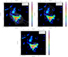 |
Fig. B.4 Outflow red emission (0.5–8 km s−1): contours of [C II] (58.5–190.2 K km s−1), 12 CO 2 →1 (3.2–46.6 K km s−1), and 12 CO 16 →15 (15.0–48.9 Kkm s−1) emission overlaid on [O I] emission in colour scale (wedge in K km s−1). |
 |
Fig. B.5 High-velocity red emission (8–25 km s−1): contours of [C II] (34.4–111.7 K km s−1) and 12 CO 2 →1 (3.1–44.4 K km s−1) emission overlaid on [O I] emission in colour scale (wedge in K km s−1). |
References
- Adams, J. D., Herter, T. L., Hora, J. L., et al. 2015, ApJ, 814, 54 [NASA ADS] [CrossRef] [Google Scholar]
- Agundez, M., Goicoechea, J. R., Cernicharo, J., et al. 2010, ApJ, 713, 662 [NASA ADS] [CrossRef] [Google Scholar]
- Andree-Labsch, S., Ossenkopf-Okada, V. Röllig, M. 2017, A&A, 598, A2 [NASA ADS] [CrossRef] [EDP Sciences] [Google Scholar]
- Asplund, M., Grevesse, N., & Sauval, A. J. 2005, ASPC, 336, 25 [Google Scholar]
- Bally, J., Snell, R. L., & Predmore, R. 1983, ApJ, 272, 154 [NASA ADS] [CrossRef] [Google Scholar]
- Balsara, D., Ward-Thompson, D., & Crutcher, R. M. 2001, MNRAS, 327, 715 [NASA ADS] [CrossRef] [Google Scholar]
- Bate, M. R. 2012, MNRAS, 419, 3115 [NASA ADS] [CrossRef] [Google Scholar]
- Beltran, M., Cesaroni, R., Neri, R., & Codella, C. 2011, A&A, 525, A151 [NASA ADS] [CrossRef] [EDP Sciences] [Google Scholar]
- Beuther, H., Schilke, P., & Menten K. M. 2002, ApJ, 566, 945 [NASA ADS] [CrossRef] [Google Scholar]
- Bieging, J. H. 1984, ApJ, 286, 591 [NASA ADS] [CrossRef] [Google Scholar]
- Bonnell, I. 2007, KITP Conference: Star Formation Then and Now, Santa Barbara, 25 [Google Scholar]
- Bontemps, S., André, P., Terebey, S., & Cabrit, S. 1996, A&A, 311, 858 [Google Scholar]
- Bontemps, S., Motte, F., Csengeri, T., & Schneider, N. 2010, A&A, 524, A18 [NASA ADS] [CrossRef] [EDP Sciences] [Google Scholar]
- Cazaux, S., & Tielens, A. G. G. M. 2002, ApJ, 575, L29 [NASA ADS] [CrossRef] [Google Scholar]
- Cazaux, S., & Tielens, A. G. G. M. 2004, ApJ, 604, 222 [NASA ADS] [CrossRef] [Google Scholar]
- Cazaux, S., & Tielens, A. G. G. M. 2010, ApJ, 715, 698 [NASA ADS] [CrossRef] [Google Scholar]
- Cohen, M., Bieging, J. H., & Welch, W. J. 1985, ApJ, 292, 249 [NASA ADS] [CrossRef] [Google Scholar]
- Comerón, F., Schneider, N., Djupvik, A. A., & Schnugg, C. 2018, A&A, 615, A2 [NASA ADS] [CrossRef] [EDP Sciences] [Google Scholar]
- Csengeri, T., Bontemps, S., Wyrowski, F., et al. 2017, A&A, 600, L10 [NASA ADS] [CrossRef] [EDP Sciences] [Google Scholar]
- Draine, B. T. 1978, ApJS, 36, 595 [NASA ADS] [CrossRef] [Google Scholar]
- Duarte-Cabral, A., Bontemps, S., Motte, F., et al. 2013, A&A, 550, A8 [NASA ADS] [CrossRef] [EDP Sciences] [Google Scholar]
- Eiroa, C., Elsässer, H., & Lahulla, J. F. 1979, A&A, 74, 89 [NASA ADS] [Google Scholar]
- Felli, M., Massi, M., Staude, H. J., et al. 1984, A&A, 135, 261 [NASA ADS] [Google Scholar]
- Furuya, R. S., Kitamura, Y., Saito, M., et al. 1999, ApJ, 525, 821 [NASA ADS] [CrossRef] [Google Scholar]
- Gibb, A. G., & Hoare, M. 2007, MNRAS, 380, 246 [NASA ADS] [CrossRef] [Google Scholar]
- Gibb, A. G., Hoare, M., Little L., & Wright M. 2003, MNRAS, 339, 1011 [NASA ADS] [CrossRef] [Google Scholar]
- Gierens, K. M., Stutzki, J., & Winnewisser, G. 1992, A&A, 259, 271 [NASA ADS] [Google Scholar]
- Guan, X., Stutzki, J., Graf, U., et al. 2012, A&A, 542, L4 [NASA ADS] [CrossRef] [EDP Sciences] [Google Scholar]
- Guillet, V., Jones, A. P., & Pineau Des Forêts, G. 2009, A&A, 497, 145 [Google Scholar]
- Gusdorf, A., Cabrit, S., Flower, D. R., & Pineau Des Forêts, G. 2008a, A&A, 482, 809 [Google Scholar]
- Gusdorf, A., Pineau Des Forêts, G., Cabrit, S., & Flower, D. R. 2008b, A&A, 490, 695 [NASA ADS] [CrossRef] [EDP Sciences] [Google Scholar]
- Guzman, A. E., Garay, G., Rodriguez, L. F., et al. 2014, ApJ, 796, 117 [NASA ADS] [CrossRef] [Google Scholar]
- Gvaramadze, V. V., & Menten, K. M. 2012, A&A, 541, A7 [NASA ADS] [CrossRef] [EDP Sciences] [Google Scholar]
- Gvaramadze, V. V., Kniazev, A. Y., & Fabrika, S. 2010, MNRAS, 405, 1047 [NASA ADS] [Google Scholar]
- Hartmann, L., Herczeg, G., & Calvet, N. 2016, Ann. Rev. Astron. Astrophs., 54, 135 [Google Scholar]
- Heiles, C. 1994, ApJ, 436, 720 [NASA ADS] [CrossRef] [Google Scholar]
- Heyminck, S., Graf, U. U., Güsten, R., et al. 2012, A&A, 542, L1 [NASA ADS] [CrossRef] [EDP Sciences] [Google Scholar]
- Hippelein, H., & Münch, G. 1981, A&A, 99, 248 [NASA ADS] [Google Scholar]
- Hoare, M., & Muxlow, T. 1996, Radio Emission from the Stars and the Sun, eds. A. R. Taylor, & J. M. Paredes (ASP), 93, 47 [NASA ADS] [Google Scholar]
- Hodapp, K., & Rayner, J. 1991, AJ, 102, 1108 [NASA ADS] [CrossRef] [Google Scholar]
- Hodapp, K., & Schneider, N. 2008, Handbook of Star Forming Regions, Vol. I, ed. B. Reipurth (The Northern Sky ASP Monograph Publications, Vol. 4), 90 [Google Scholar]
- Hollenbach, D. 1985, Icarus, 61, 36 [NASA ADS] [CrossRef] [Google Scholar]
- Hollenbach, D., & McKee, C. F. 1989, ApJ, 342, 306 [NASA ADS] [CrossRef] [Google Scholar]
- Hollenbach, D., Kaufman, M. J., Neufeld, D., et al. 2012, ApJ, 754, 105 [NASA ADS] [CrossRef] [Google Scholar]
- Hunter, T. R., Brogan, C. L., Indebetouw, R., et al. 2008, ApJ, 680, 1271 [NASA ADS] [CrossRef] [Google Scholar]
- Kirk, H., Myers, P. C., Bourke, T. L., et al. 2013, ApJ, 766, 115 [NASA ADS] [CrossRef] [Google Scholar]
- Kristensen, L. E., van Dishoeck, E. F., Mottram, J. C., et al. 2017, A&A, 605, A93 [NASA ADS] [CrossRef] [EDP Sciences] [Google Scholar]
- Kuiper, R., Klahr, H., Beuther, H., & Henning, T. 2011, ApJ, 732, 20 [NASA ADS] [CrossRef] [Google Scholar]
- Kuruwita, R., Federrath, C., & Ireland, M. 2017, MNRAS, 470, 1626 [NASA ADS] [CrossRef] [Google Scholar]
- Langer, W. D., & Penzias, A. A. 1990, ApJ, 357, 477 [NASA ADS] [CrossRef] [Google Scholar]
- Larson, R. B. 1981, MNRAS, 194, 809 [NASA ADS] [CrossRef] [Google Scholar]
- Leurini, S., Wyrowski, F., Wiesemayer, H., et al. 2015, A&A, 584, A70 [NASA ADS] [CrossRef] [EDP Sciences] [Google Scholar]
- Liseau, R., Justtanot, K., & Tielens, A. G. G. M. 2006, A&A, 446, 561 [NASA ADS] [CrossRef] [EDP Sciences] [Google Scholar]
- Lesaffre, P., Pineau des Forêts, G., Godard, B., et al. 2013, A&A, 550, A106 [NASA ADS] [CrossRef] [EDP Sciences] [Google Scholar]
- Little, L. T., Kelly, M. L., Habing, R., et al. 1995, MNRAS, 277, 307 [NASA ADS] [Google Scholar]
- Mathis, J. S., Rumpl, W., & Nordsieck, K. H. 1977, ApJ, 217, 425 [NASA ADS] [CrossRef] [Google Scholar]
- Maud, L. T., Moore, T. J. T., Lumsden, S. L., et al. 2015, MNRAS, 453, 645 [NASA ADS] [CrossRef] [Google Scholar]
- McElroy, D., Walsh, C., & Markwick, A. J. 2013, A&A, 550, A36 [NASA ADS] [CrossRef] [EDP Sciences] [Google Scholar]
- McKee, C. F., & Tan, J. C. 2002, Nature, 416, 59 [NASA ADS] [CrossRef] [PubMed] [Google Scholar]
- Minier, V., Tremblin, P., Hill, T., et al. 2013, A&A, 550, A50 [NASA ADS] [CrossRef] [EDP Sciences] [Google Scholar]
- Motte, F., Bontemps, S., Schilke, P., et al. 2007, A&A, 476, 1243 [NASA ADS] [CrossRef] [EDP Sciences] [Google Scholar]
- Nagy, Z., Van der Tak, F. F. S., & Ossenkopf, V. 2013, A&A, 550, A96 [NASA ADS] [CrossRef] [EDP Sciences] [Google Scholar]
- Nisini, B., Santangelo, G., Giannini, T., et al. 2015, ApJ, 801, 121 [NASA ADS] [CrossRef] [EDP Sciences] [Google Scholar]
- Noel, B., Joblin, C., Maillard, J. P., & Paumard, T. 2005, A&A, 436, 569 [NASA ADS] [CrossRef] [EDP Sciences] [Google Scholar]
- Oasa, Y., Tamura, M., Nakajima, Y., et al. 2006, AJ, 131, 1608 [NASA ADS] [CrossRef] [Google Scholar]
- Peretto, N., Fuller, G. A., Duarte-Cabral, A., et al. 2013, A&A, 555, A112 [NASA ADS] [CrossRef] [EDP Sciences] [Google Scholar]
- Peters, T., Klessen, R. S., Mac Low, M.-M., et al. 2010a, ApJ, 725, 134 [NASA ADS] [CrossRef] [Google Scholar]
- Peters, T., Banerjee, R., Klessen, R. S., et al. 2010b, ApJ, 711, 1017 [NASA ADS] [CrossRef] [Google Scholar]
- Peters, T., Banerjee, R., Klessen, R. S., et al. 2011, ApJ, 729, 72 [NASA ADS] [CrossRef] [Google Scholar]
- Polehampton, E. T., Baluteau, J.-P., & Swinyard, B. M. 2005, A&A, 437, 957 [NASA ADS] [CrossRef] [EDP Sciences] [Google Scholar]
- Rayner, T., Griffin, M., Schneider, N., et al. 2017, A&A, 607, A22 [NASA ADS] [CrossRef] [EDP Sciences] [Google Scholar]
- Richer, J., Padman, R., Ward-Thompson, D., et al. 1993, MNRAS, 262, 839 [NASA ADS] [CrossRef] [Google Scholar]
- Riera, A., Mampaso, A., Vilchez, J. M., & Phillips, J. P. 1989, A&A, 210, 351 [NASA ADS] [Google Scholar]
- Röllig, M. 2011, A&A, 530, A9 [NASA ADS] [CrossRef] [EDP Sciences] [Google Scholar]
- Röllig, M., & Ossenkopf, V. 2013, A&A, 550, A56 [NASA ADS] [CrossRef] [EDP Sciences] [Google Scholar]
- Röllig, M., Ossenkopf, V., Jeyakumar, S., et al. 2006, A&A, 451, 917 [NASA ADS] [CrossRef] [EDP Sciences] [Google Scholar]
- Röllig, M., Abel, N. P., Bell, T., et al. 2007, A&A, 467, 187 [NASA ADS] [CrossRef] [EDP Sciences] [Google Scholar]
- Röllig, M., Szczerba, R., Ossenkopf, V., & Glück, C. 2013, A&A, 549, A85 [NASA ADS] [CrossRef] [EDP Sciences] [Google Scholar]
- Sanchez-Monge, A., Cesaroni, R., Beltran, M. T., et al. 2013, A&A, 552, L10 [NASA ADS] [CrossRef] [EDP Sciences] [Google Scholar]
- Schilke, P., Walmsley, C. M., Pineau des Forets, G., & Flower, D. R. 1997, A&A, 321, 293 [NASA ADS] [Google Scholar]
- Schneider, N., Simon, R., Kramer, C., Stutzki, J., & Bontemps, S. 2002, A&A, 384, 225 [NASA ADS] [CrossRef] [EDP Sciences] [Google Scholar]
- Schneider, N., Simon, R., Kramer, C., et al. 2003, A&A, 406, 915 [NASA ADS] [CrossRef] [EDP Sciences] [Google Scholar]
- Schneider, N., Simon, R., Bontemps, S., et al. 2007, A&A, 474, 873 [NASA ADS] [CrossRef] [EDP Sciences] [Google Scholar]
- Schneider, N., Csengeri, T., Bontemps, S., et al. 2010, A&A, 520, A49 [NASA ADS] [CrossRef] [EDP Sciences] [Google Scholar]
- Schneider, N., Bontemps, S., Motte, F., et al. 2016, A&A, 591, A40 [NASA ADS] [CrossRef] [EDP Sciences] [Google Scholar]
- Solf, J., & Carsenty, U. 1982, A&A, 116, 54 [NASA ADS] [Google Scholar]
- Simon, M., & Fischer, J. 1982, BAAS, 14, 925 [NASA ADS] [Google Scholar]
- Simon, R. Schneider, N., Stutzki, J., et al. 2012, A&A, 542, L12 [NASA ADS] [CrossRef] [EDP Sciences] [Google Scholar]
- Simon-Diaz, S., & Stasinska, G. 2011, A&A, 526, A48 [NASA ADS] [CrossRef] [EDP Sciences] [Google Scholar]
- Stock, D., Wolfire, M., Peeters, E., et al. 2015, A&A, 579, A67 [NASA ADS] [CrossRef] [EDP Sciences] [Google Scholar]
- Störzer, H., & Hollenbach, D. 1998, ApJ, 495, 853 [NASA ADS] [CrossRef] [Google Scholar]
- Störzer, H., Stutzki, J., & Sternberg, A. 1996, A&A, 310, 592 [NASA ADS] [Google Scholar]
- Stutzki, J., Ungerechts, H., & Winnewisser, G. 1982, A&A, 111, 201 [NASA ADS] [Google Scholar]
- Szczerba, R., Omont, A., Volk, K., et al. 1997, A&A, 317, 859 [NASA ADS] [Google Scholar]
- Tan, J. C., Kong, S., Butler, M., et al. 2013, ApJ, 779, 96 [NASA ADS] [CrossRef] [Google Scholar]
- Tan, J. C., Beltran, M. T., Caselli, P., et al. 2014, Protostars and Planets VI, eds. H. Beuther, R. S. Klessen, C. P. Dullemond, T. Henning (Tucson: University of Arizona Press), 914, 149 [NASA ADS] [Google Scholar]
- Vallée, J. P., & Fiege, J. D. 2005, ApJ, 627, 263 [NASA ADS] [CrossRef] [Google Scholar]
- van den Ancker, M., Tielens, A. G. G. M., & Wesselius, P. 2000, A&A, 111, 201 [Google Scholar]
- Visser, R., vanDishoeck, E. F., & Black, J. H. 2009, A&A, 503, 323 [NASA ADS] [CrossRef] [EDP Sciences] [Google Scholar]
- Weingartner, J. C., & Draine, B. T. 2001a, ApJ, 548, 296 [NASA ADS] [CrossRef] [Google Scholar]
- Weingartner, J. C., & Draine, B. T. 2001b, ApJS, 134, 263 [NASA ADS] [CrossRef] [MathSciNet] [Google Scholar]
- Wyrowski, F., Güsten, R., Menten, K. M., et al. 2012, A&A, 542, L15 [NASA ADS] [CrossRef] [EDP Sciences] [Google Scholar]
- Xu, Y., Li, J. J., Reid, M.J., et al. 2013, ApJ, 769, 15 [NASA ADS] [CrossRef] [Google Scholar]
German Receiver for Astronomy at Terahertz. GREAT is a development by the MPI für Radioastronomie and the KOSMA/Universität zu Köln, in cooperation with the MPI für Sonnensystemforschung and the DLR Institut für Planetenforschung.
IRAM is supported by INSU/CNRS (France), MPG (Germany), and IGN (Spain).
The KOSMA-τ code was part of the PDR comparison benchmark study (Röllig et al. 2007).
All ratios are computed from intensities in erg s−1 cm−2 sr−1. See Table 2 for conversion factors.
To convert the FORCAST data from MJy pixel−1 to MJy sr−1 we use the conversion factor 7.213 × 1010 pixel sr−1.
As already discussed and shown in more detail in Schneider et al. (2003), the dip seen in [O I], [C II], and 12CO 2 →1 spectra gets filled in with emission in the corresponding 13CO 2 →1 spectra. The ratio 12CO/13CO drops to values lower than 1 for this velocity range over a large area on the western side of S106 IR (see Fig. 8 in Schneider et al. 2003). The lack of 12CO (and [O I] and [C II]) emission around +3 km s−1 is thus due to absorption of these lines becoming optically thick in cold foreground material. This cold gas originates from a molecular clump, associated with the extended molecular cloud.
As a consistency check, we determined the total [O I] 63 μm and [C II] 158 μm line intensity in a 40″ beam around the position of S106 IR and compared it to the value obtained with Herschel (Stock et al. 2015). Our line intensities are slightly lower but agree well, considering the calibration uncertainties for both instruments (15–20%). Our values of [O I] and [C II] emission are 2.2 × 10⁻² and 3.6 × 10⁻³ erg cm−2 sr−1 s−1, respectively, compared to 2.9 × 10⁻² and 3.9 × 10⁻³ erg cm−2 sr−1 s−1 from Stock et al. (2015).
An independent measure of the radiation field is to use the Herschel fluxes at 70 and 160 μm (see e.g. Schneider et al. 2016). With this method, we obtained a field of typically χ = 2–4 × 10⁴ or S106.
The visual extinction in the lane has been estimated between Av = 12 and 21 mag (Eiroa et al. 1979; Hodapp & Rayner 1991; van den Ancker et al. 2000).
See also the animated version of this cartoon available online.
We talk here of a parsec-scale flow that connects the molecular cloud with the disk(s) or the remains thereof, and not of possible sub-pc flows that channel material from the disk(s) onto the star (Sect. 5.1.1).
All Tables
All Figures
|
Fig. 1 Near-IR image (filters at J (1.25 μm), H (1.65 μm), and K′ (2.15 μm)) of S106 taken with Subaru (Oasa et al. 2006), outlining the bipolar emission nebula, with contours of velocity integrated (–30 to 25 km s−1) [O I] emission (136 to 456 K km s−1 in steps of 64 K km s−1). The area mapped with SOFIA in [O I] and CO 16 →15 emission is indicated with a white polygon. The star indicates the position of the S106 IR binary system and the triangle the position of the young stellar object (YSO) S106 FIR. |
| In the text | |
|
Fig. 2 Schematic view of the S106 region as seen on the sky. The nebula is tilted ≈25° to the east in the plane of the sky; the northern lobe, which is more obscured by foreground gas and dust, is inclined (≈15°) away from the observer. The southern lobe is inclined towards the observer and lacks the front side. The bipolar nebula and the H II region are embedded in an extended molecular cloud. |
| In the text | |
|
Fig. 3 One example (position 3a, southern cavity) for KOSMA-τ PDR model continuum emission fitting the observed continuum observations (black points) of MAMBO (1.2 mm), Herschel (PACS: 70, 160, SPIRE: 250 μm), and FORCAST (19.7, 25.3, 31.5, 37.1 μm), assuming a unity beam filling factor. The error for the flux values is generally small (see Sect. 2.2). All data were smoothed to a common angular resolution of 15″. The Herschel/SPIRE 250 μm data point has a resolution of 18″. |
| In the text | |
|
Fig. 4 Spectral map of [O I] emission with a velocity resolution of 1 km s−1 on a 6″ beam-sampled grid in the velocity range from –40 to 40 km s−1 and main beam brightness temperature range from –4 to 40 K. |
| In the text | |
|
Fig. 5 Spatially averaged spectrum of molecular and atomic lines (the spectral resolution is typically 0.2–0.6 km s−1). All spectra within the central area of 40″ × 40″ around S106 IR were included. Based upon the different spectral features, we define five major velocity ranges. The local standard of rest (lsr) velocity of the S106 molecular cloud is approximately –3 km s−1. |
| In the text | |
|
Fig. 6 [O I] emission of the total velocity range from –30 to 25 km s−1 in contours overlaid on a map of 19 μm emission (FORCAST; Adams et al. 2015). Positions for which we show individual spectra of various lines and report the line integrated intensities in Table 2 (in a 15″ beam) are indicated with a cross and labelled 1–6. The angular resolution of the 19 μm emissionand the [O I] beam are indicated in the panel. For comparison, the 15″ resolution we used for PDR modelling is also given. Positions 1–6 do not always correspond to peaks in [O I] emission, but also to peak emission in high- and low-J CO lines (see text for details). |
| In the text | |
 |
Fig. 7 Individual spectra with 15″ angular resolution at the positions indicated in Fig. 5. |
| In the text | |
|
Fig. 8 Channel map of [O I] emission in 2 km s−1 velocity bins. The contour levels are 5, 10, 20, 45, and 60 K km s−1. The logarithmic colour scale ranges from 1.5 to 60 K km s−1. The star indicates the binary system S106 IR and the triangle S106 FIR. |
| In the text | |
|
Fig. 9 PDR diagnostic diagrams for observed fine-structure lines based on the KOSMA-τ PDR model for a clump of M = 100 M⊙.
|
| In the text | |
|
Fig. 10 PDR diagnostic diagrams for observed fine-structure lines based on the KOSMA-τ PDR model for a clump of M = 100 M⊙. CO(16–15)/CO(11–10) against |
| In the text | |
|
Fig. 11 [O I] line integrated emission overlayed as contours on 19 μm emission from dust (Adams et al. 2015). The left panel shows the high-velocity blue emission and the right panel the high-velocity red emission. The dust emission ranges between 0 and 2.6 Jy pix−1, the [O I] contour lines go from 30 to 100% of maximum intensity (397 K km s−1 for HV-blue and 121 K km s−1 for HV-red). |
| In the text | |
|
Fig. 12 [O I] line integrated emission overlayed as contours on cm emission from the VLA (Bally et al. 1983). The left panel shows the blue outflow range and the right panel the redemission. The [O I] contour lines go from 36 to 156 in steps of 10 K km s−1 for the blue outflow and 40 to 180 in steps of 10 K km s−1 for the red outflow. The star indicates the binary system S106 IR and the triangle S106 FIR. |
| In the text | |
|
Fig. 13 Optical image from the Gran Telescopio Canaries (colour) with an overlay of CO 16 →15 line integrated emission (contour levels 18.6 to 83.8 in steps of 6.5 K km s−1) in the blue outflow velocity range (–9 to –4 km s−1). The dark lane is indicated by one black contour (3 Jy) of SHARC 350 μm emission (see Fig. 13). |
| In the text | |
|
Fig. 14 SHARC 350 μm emission (colour wedge in Jy) with overlays of CO 16 →15 line integrated emission (levels 14 to 47 by 3 K km s−1, grey contours) in the bulk velocity range (–4 to 0.5 km s−1). |
| In the text | |
|
Fig. 15 Channel map of H13CO+ 1 →0 emission (contours in K km s−1 from 0.25 to 1.75 in steps of 0.25) obtained with the IRAM 30 m telescope. The background image is the Subaru IR image from Fig 1. The blue contour is the 3 Jy level of the SHARC 350 μm emission. The star marks the position of the binary system S106 IR; the dashed red line indicates the run of the dark lane, i.e. thepossible accretion flow. |
| In the text | |
|
Fig. 16 Schematic view of two possible scenarios (shown at the same time) explaining the nature of the dark lane. The front view (left panel), as S106 is seen on the sky, does not allow us to distinguish between infall scenario (dark lane in green) or expansion scenario (dark lane in blue) of the gas in the dark lane. The middle view shows best the “accretion flow” scenario, i.e. how the (green) dark lane wraps around the equatorial waist of the hourglass-nebula. The right view shows how the (blue) dark lane, which is more detached from the nebula, is tilted towards the observer and dispersed. An animated version of this cartoon is available online. |
| In the text | |
|
Fig. B.1 High-velocity blue emission (–30 to –9 km s−1): contours of [C II] (30–100 K km s−1), and 12 CO 2 →1 (3.1–44.4 K km s−1) emission overlaid on [O I] emission in colour scale (wedge in K km s−1). |
| In the text | |
|
Fig. B.2 Outflow blue emission (–9 to –4 km s−1): contours of [C II] (59–192 K km s−1), 12 CO 2 →1 (3.1–44.4 K km s−1), 12 CO 16 →15 (13.1–191.1 K km s−1), and 13 CO 2 →1 (2.0–28.9 K km s−1) emission overlaid on [O I] emission in colour scale (wedge in K km s−1). |
| In the text | |
|
Fig. B.3 Molecular cloud bulk emission (–4 to 0.5 km s−1): contours of [C II] (72.5–235.5 K km s−1), 12 CO 2 →1 (24.7–357.8 K km s−1), 12 CO 16 →15 (9.5–66.9 K km s−1), and 13 CO 2 →1 (5.8 to 84.5 K km s−1) emission overlaid on [O I] emission in colour scale (wedge in K km s−1). |
| In the text | |
|
Fig. B.4 Outflow red emission (0.5–8 km s−1): contours of [C II] (58.5–190.2 K km s−1), 12 CO 2 →1 (3.2–46.6 K km s−1), and 12 CO 16 →15 (15.0–48.9 Kkm s−1) emission overlaid on [O I] emission in colour scale (wedge in K km s−1). |
| In the text | |
|
Fig. B.5 High-velocity red emission (8–25 km s−1): contours of [C II] (34.4–111.7 K km s−1) and 12 CO 2 →1 (3.1–44.4 K km s−1) emission overlaid on [O I] emission in colour scale (wedge in K km s−1). |
| In the text | |
Current usage metrics show cumulative count of Article Views (full-text article views including HTML views, PDF and ePub downloads, according to the available data) and Abstracts Views on Vision4Press platform.
Data correspond to usage on the plateform after 2015. The current usage metrics is available 48-96 hours after online publication and is updated daily on week days.
Initial download of the metrics may take a while.