| Issue |
A&A
Volume 617, September 2018
|
|
|---|---|---|
| Article Number | A27 | |
| Number of page(s) | 36 | |
| Section | Interstellar and circumstellar matter | |
| DOI | https://doi.org/10.1051/0004-6361/201731159 | |
| Published online | 12 September 2018 | |
Kinematics of dense gas in the L1495 filament★,★★
1
Max-Planck-Institut für extraterrestrische Physik,
Giessenbachstrasse 1,
85748
Garching,
Germany
2
Ural Federal University,
19 Mira St.,
620002
Yekaterinburg,
Russia
e-mail: This email address is being protected from spambots. You need JavaScript enabled to view it.
3
Department of Physics and Astronomy, The University of Western Ontario,
1151 Richmond Street,
London,
ON
N6A 3K7,
Canada
4
Observatorio Astronómico Nacional (IGN),
Alfonso XII 3,
28014
Madrid,
Spain
5
Leiden Observatory, University of Leiden,
Niels Bohrweg 2,
2333
CA Leiden,
The Netherlands
Received:
11
May
2017
Accepted:
12
June
2018
Abstract
Context. Nitrogen bearing species, such as NH3, N2H+, and their deuterated isotopologues show enhanced abundances in CO-depleted gas, and thus are perfect tracers of dense and cold gas in star-forming regions. The Taurus molecular cloud contains the long L1495 filament providing an excellent opportunity to study the process of star formation in filamentary environments.
Aims. We study the kinematics of the dense gas of starless and protostellar cores traced by the N2D+(2–1), N2H+(1–0), DCO+(2–1), and H13CO+(1–0) transitions along the L1495 filament and the kinematic links between the cores and surrounding molecular cloud.
Methods. We measured velocity dispersions, local and total velocity gradients, and estimate the specific angular momenta of 13 dense cores in the four transitions using on-the-fly observations with the IRAM 30-m antenna. To study a possible connection to the filament gas, we used the C18O(1–0) observations.
Results. The velocity dispersions of all studied cores are mostly subsonic in all four transitions and are similar and almost constant dispersion across the cores in N2D+(2–1) and N2H+(1–0). A small fraction of the DCO+(2–1) and H13CO+(1–0) lines show transonic dispersion and exhibit a general increase in velocity dispersion with line intensity. All cores have velocity gradients (0.6–6.1 km s−1 pc−1), typical of dense cores in low-mass star-forming regions. All cores show similar velocity patterns in the different transitions, simple in isolated starless cores, and complex in protostellar cores and starless cores close to young stellar objects where gas motions can be affected by outflows. The large-scale velocity field traced by C18O(1–0) does not show any perturbation due to protostellar feedback and does not mimic the local variations seen in the other four tracers. Specific angular momentum J∕M varies in a range (0.6–21.0) × 1020 cm2 s−1, which is similar to the results previously obtained for dense cores. The J∕M measured in N2D+(2–1) is systematically lower than J∕M measured in DCO+(2–1) and H13CO+(1–0).
Conclusions. All cores show similar properties along the 10 pc-long filament. N2D+(2–1) shows the most centrally concentrated structure, followed by N2H+(1–0) and DCO+(2–1), which show similar spatial extent, and H13CO+(1–0). The non-thermal contribution to the velocity dispersion increases from higher to lower density tracers. The change of magnitude and direction of the total velocity gradients depending on the tracer used indicates that internal motions change at different depths within the cloud. N2D+ and N2H+ show smaller gradients than the lower density tracers DCO+ and H13CO+, implying a loss of specific angular momentum at small scales. At the level of cloud-core transition, the core’s external envelope traced by DCO+ and H13CO+ is spinning up, which is consistent with conservation of angular momentum during core contraction. C18O traces the more extended cloud material whose kinematics is not affected by the presence of dense cores. The decrease in specific angular momentum towards the centres of the cores shows the importance of local magnetic fields to the small-scale dynamics of the cores. The random distributions of angles between the total velocity gradient and large-scale magnetic field suggests that magnetic fields may become important only in high density gas within dense cores.
Key words: stars: formation / ISM: kinematics and dynamics / ISM: clouds / ISM: molecules / ISM: individual objects: L1495 / radio lines: ISM
This work is based on observations carried out under the projects 032-14 and 156-14 with the IRAM 30 m Telescope. IRAM is supported by INSU/CNRS (France), MPG (Germany), and IGN (Spain).
The data cubes with the hfs parameters are only available at the CDS via anonymous ftp to cdsarc.u-strasbg.fr (130.79.128.5) or via http://cdsarc.u-strasbg.fr/viz-bin/qcat?J/A+A/617/A27
© ESO 2018
1 Introduction
Recent submillimetre studies of the nearest star-forming clouds with the Herschel Space Observatory show that interstellar filaments are common structures in molecular clouds and play an important role in the star-forming process (e.g. Men’shchikov et al. 2010; André et al. 2014). The filaments host chains of dense cores (e.g. Hacar et al. 2013; Könyves et al. 2014); some of the cores are pre-stellar, on the verge of star formation. Pre-stellar cores are cold (~10 K), dense (104 –107 cm−3), and quiescent (thermal pressure dominates turbulent motions; e.g. Benson & Myers 1989; Fuller & Myers 1992; Lada et al. 2008; Caselli et al. 2008)self-gravitating structures (Ward-Thompson et al. 1999; Keto & Caselli 2008) that are characterized by high deuterium fractions (>10%; Crapsi et al. 2005). Pre-stellar cores represent the initial conditions in the process of star formation, thus their study is crucial to understand how stars and stellar systems form.
The target of our study, L1495 (Lynds 1962), is an extended filamentary structure in the Taurus molecular cloud, a nearby (140 pc distance; Elias 1978; Torres et al. 2012), relatively quiescent, low-mass star-forming region. The selected filament contains 39 dense cores revealed in ammonia by Seo et al. (2015) including 19 dense cores previously detected in N2H+(1–0) emission (Hacar et al. 2013; see Fig. 1) at different stages of star formation. Tens of starless cores are detected there via continuum emission by Herschel (Marsh et al. 2014), and about 50 low-mass protostars in different evolutionary stages were observed with Spitzer (see the survey by Rebull et al. 2010). L1495 is a very well-studied region; its physical properties and structure are determined by several large observational studies. This includes its gas kinetic temperature(Seo et al. 2015); dust extinction (Schmalzl et al. 2010); low density gas distribution, as traced by H13CO+ (Onishi et al. 2002) and C18O (Hacar et al. 2013); and dense gas distribution and dense cores locations, as traced by N2H+ (Hacar et al. 2013; Tafalla & Hacar 2015) and NH3 (Seo et al. 2015). Thus, L1495 is an excellent place to test theories of dense core formation within filaments.
Hacar et al. (2013) mapped the whole filament in C18O(1–0), SO(3–2), and N2H+(1–0) using the Five College Radio Astronomy Observatory (FCRAO) antenna. These authors found that the filament is not a uniform structure and consists of many fibres. The fibres are elongated structures mostly aligned with the axis of the large-scale filament and have typical lengths of 0.5 pc, coherent velocity fields, and internal velocity dispersions close to the sound speed. The fibres were revealed in the low density gas tracer C18O(1–0) kinematically, that is the Gaussian fits of the multiple C18O(1–0) components plotted in position-position-velocity space appear as velocity coherent structures. Their distribution resembles the small-scale structures revealed with the getfilaments algorithm (Men’shchikov 2013) in Herschel dust continuum emission when large-scale emission was filtered out (André et al. 2014). Some of the CO fibres contain dense cores revealed by the high density tracer N2H+(1–0). Hacar et al. (2013) concluded that fragmentation in the L1495 complex proceeded in a hierarchical manner, from cloud to subregions (bundles) to fibres and then to individual dense cores. In the following study, Tafalla & Hacar (2015) found that the cores tend to cluster in linear groups (chains). Hacar et al. (2013) and Seo et al. (2015) noted that some parts of the filament are young (B211 and B216) and others (B213 and B7) are more evolved and actively star forming. The gas temperature derived by Seo et al. (2015) from NH3 is low, 8–15 K with a median value of 9.5 K, and less evolved (B10, B211, and B216) regions only have a median temperature 0.5 K less than more evolved (B7, B213, B218) regions. These authors found that the gas kinetic temperature decreases towards dense core centres. With NH3, which traces less dense gas than N2H+, Seo et al. (2015) found 39 ammonia peaks including those 19 found by Hacar et al. (2013). Onishi et al. (2002) presented a large survey of H13CO+(1–0) observed towards C18O emission peaks in L1495.
Previous studies of the gas kinematics in L1495 were focussed on the large-scale structure, the filament as a whole, and its subregions. We focus on the kinematics within the dense gas of the cores traced by N2H+ and N2D+ and the kinematics of the surrounding core envelope traced by H13CO+ and DCO+ to study the gas that connects the cores to their host cloud.
The best tracers of the dense gas kinematics are N-bearing species. In dense (> a few × 104 cm−3) and cold (T ≃ 10 K) regions, CO, CS, and other C-bearing species are heavily frozen onto dust grains (Caselli et al. 1999; Tafalla et al. 2006; Bizzocchi et al. 2014). Nitrogen-bearing species such as N2H+ and NH3 and their deuterated isotopologues stay in the gas phase up to densities of 106 cm−3 (Crapsi et al. 2005, 2007) and become good tracers of dense gas (see also Tafalla et al. 2004). N2H+ rotational transitions have higher critical densities (ncrit ≥ 105 cm−3) than the inversion transitions of NH3 (ncrit ~ 103 cm−3) and thus N2H+ traces dense gas better than NH3. Deuterated species also increase their abundance towards the central regions of cores because of the enhanced formation rate of deuterated forms of H , for example H2 D+ (the precursor of deuterated species, such as DCO+, N2D+, and deuterated ammonia), in zones where CO is mostly frozen onto dust grains (e.g. Dalgarno & Lepp 1984; Caselli et al. 2003). To study the kinematics of the gas in the central parts of the cores, we choose the N2D+(2–1) transition (ncrit = 2.5 × 106 cm−3, calculated using the data1 from the LAMDA database; Schöier et al. 2005), and the N2H+(1–0) line to connect to the work of Hacar et al. (2013), who also mapped N2H+(1–0), and also to study the deuterium fraction across the cores, which will be presented in a subsequent study (Punanova et al., in prep.). HCO+ follows CO and thus it depletes in the centres of dense cores (e.g. Pon et al. 2009); therefore, HCO+ is a good tracer of core envelopes. To study the kinematics of the core surroundings and provide a connection between the kinematics of the cores and that of the cloud, we choose the H13CO+(1–0) and DCO+(2–1) transitions. This will also enable a future study of the deuterium fraction of the cores and core envelopes (Punanova et al., in prep.).
This paper presents observations of N2D+(2–1), N2H+(1–0), DCO+(2–1), and H13CO+(1–0) towards 13 dense cores to study the kinematics of the dense gas along the L1495 filament. In Sect. 2, the details of the observations are presented. Section 3 describes the data reduction procedure. Section 4 presents the results of the hfs fitting and velocity gradients and specific angular momenta calculations. In Sect. 5 we discuss the results and connections between core-scale and cloud-scale kinematics. The conclusions are given in Sect. 6.
2 Observations
We mapped 13 out of 19 dense cores of the L1495 filamentary structure (see Fig. 1 and Table 1) in N2D+(2–1) at 154.2 GHz, N2H+(1–0) at 93.2 GHz, DCO+(2–1) at 144.1 GHz, and H13CO+(1–0) at 86.8 GHz with the IRAM 30 m telescope (IRAM projects 032-14 and 156-14). The D13CO+(2–1) at 141.5 GHz and HC18O+(1–0) at 85.2 GHzlines were observed towards the DCO+(2–1) emission peaks of 9 cores. The observations were performed on 09–14 July, 02–08 December 2014, and 04 June 2015 under acceptable weather conditions, pwv = 1–9 mm. The on-the-fly maps and single pointing observationswere obtained with the EMIR 090 (3 mm band) and EMIR 150 (2 mm band) heterodyne receivers2 in position switching mode, and the VESPA backend. The spectral resolution was 20 kHz, the corresponding velocity resolutions were ≃0.07 for the 3 mm band and ≃0.04 km s−1 for the 2 mm. The beam sizes were ≃28′′ for the 3 mm band and ≃17′′ for the 2 mm band. The system temperatures were 90–627 K depending on the lines. The exact line frequencies, beam efficiencies, beam sizes, spectral resolutions, and sensitivities are given in Table 2. Sky calibrations were obtained every 10–15 min. Reference positions were chosen individually for each core to make sure that the positions were free of N2H+(1–0) emission, using the Hacar et al. (2013) maps. The reference position for core 4 was contaminated with N2H+(1–0) emission, thus it is not analysed in the paper. Pointing was checked by observing QSO B0316+413, QSO B0415+379, Uranus, and Venus every two hours and focus was checked by observing Uranus and Venus every six hours.
To connect core-scale and cloud-scale kinematics, we used the fit results of the C18O(1–0) observations by Hacar et al. (2013) convolved to 60′′, performed with the 14 m FCRAO telescope.
Observed cores.
Observation parameters.
3 Data reduction and analysis with Pyspeckit
The data reduction up to the stage of convolved spectral data cubes was performed with the CLASS package3. The intensity scale was converted to the main-beam temperature scale according to the beam efficiency values4 (see Table 2 for details). The N2H+(1–0) maps were convolved to a resolution of 27.8′′ with 9′′ pixel size. The N2D+(2–1) maps were convolved to the resolution of the N2H+(1–0) with the same grid spacing to improve the sensitivity for a fair comparison of the kinematics traced by these transitions. The H13CO+(1–0) and DCO+(2–1) maps were convolved to resolutions of 29.9′′ and 18′′ with pixel sizes of 9′′ and 6′′, respectively. The rms across the maps in Tmb scale is 0.075–0.14 K, 0.04–0.10 K, 0.11–0.21 K, and 0.15–0.50 K for the N2H+(1–0), N2D+(2–1), H13CO+(1–0), and DCO+(2–1), respectively. Each map has a different sensitivity (see Table A.3 for details). The undersampled edges of the maps are not used for the analysis. Each data cube contains spectra of one transition towards one core. Some cores lie close to each other so we also produced combined data cubes (cores 4 and 6 and the chain of cores 10–13; see e.g. Figs. 1 and A.8). Another dataset with all maps convolved to the biggest beam (29.9′′) and Nyquist sampling was produced to compare local and total velocity gradients across the cores seen in different species (see Sect. 4.5.2 for details). The rms in Tmb scale across the maps smoothed to29.9′′ is in the ranges 0.065 – 0.12 K, 0.04–0.085 K, 0.11–0.21 K, and 0.05–0.15 K for the N2H+(1–0), N2D+(2–1), H13CO+(1–0), and DCO+(2–1), respectively (see Table A.4 for details).
The spectral analysis was performed with the Pyspeckit module of Python (Ginsburg & Mirocha 2011). The N2H+(1–0), N2D+(2–1), H13CO+(1–0), and DCO+(2–1) lines have hyperfine splitting with 15, 40, 6, and 6 components, respectively. Thus we performed hyperfine structure (hfs) fitting using the standard routines of Pyspeckit. The routine computes line profiles with the assumptions of Gaussian velocity distributions and equal excitation temperatures for all hyperfine components. It varies four parameters (excitation temperature Tex, optical depth τ, central velocity of the main hyperfine component VLSR, and velocity dispersion σ) and finds the best fit with the Levenberg–Marquardt non-linear regression algorithm. The rest frequencies of the main components, the velocity offsets, and the relative intensities of the hyperfine components were taken from Pagani et al. (2009), Schmid-Burgk et al. (2004), Caselli & Dore (2005), and Dore (priv. comm.). For the spectra of each transition towards the N2H+(1–0) emission peak of core 2, the results of Pyspeckit hfs fitting procedure were compared to the results of the CLASS hfs fitting method. The results agree within the errors. We first fitted Gaussians to the H13CO+(1–0) and DCO+(2–1) lines and compared the results to the hfs fit results. We found that the hyperfine structure significantly affects the line profile and should be taken into account to provide accurate linewidths (see Appendix A.1 for details).
The general data fitting procedure went as follows. First each spectrum in one data cube (one core, one species) was fitted two times assuming 1) unconstrained τ (all four parameters Tex, τ, VLSR, and σ were free) and 2) constrained τ (τ was fixed at0.1, which makes the fit close to the assumption that the line is optically thin; the other three parameters were free). Second, the final results data cube was produced by combining the results of the τ-constrained and τ-unconstrained fits. If τ∕Δτ ≥ 3, where Δτ is the optical depth uncertainty, the results of the τ-unconstrained fit were written to the final result data cube. If τ∕Δτ < 3, the τ-constrained fit was chosen and written to the final result data cube. The τ∕Δτ test was carried out for each pixel. The combination of τ-constrained and τ-unconstrained fits does notcause any sharp change in the velocity dispersion and centroid velocity maps, although it leads to a small increase (≃ 0.02 km s−1) in velocity dispersion for some cores (see e.g. cores 6 and 8 in Fig. A.9). One can see how constrained opacity affects the fit comparing Figs. A.9 and A.11, in which we show only the opacity maps that have more than three pixels with τ-unconstrained fit. The combined results data cube was written to the final fits file after masking poor data. For the integrated intensity maps, we used all data except the undersampled edges of the maps. The excitation temperatureand the optical depth were measured only for those spectra with a high signal-to-noise ratio (S/N):  , where I is the integrated intensity, Nch is the number of channels in the line, and Δvres is the velocity resolution. For Nch, we take all channels in the ranges 2–12, –4–16, 5–10, and 5–10 km s−1 for N2D+(2–1), N2H+(1–0), and DCO+(2–1) and H13CO+(1–0), respectively. These ranges define the emission above one
  over spectrum averaged over the whole mapped area. For the central velocity and velocity dispersion maps we used the S/N mask and a mask based on velocity dispersion: the minimum linewidth must be larger than the thermal linewidth (σT) for a temperature of 5 K (slightly below the minimum gas temperature in L1495 found by Seo et al. 2015), which is 0.04 km s−1 for the given species, and the linewidth must be defined with an accuracy better than 20% (σ∕Δσ > 5). If the line is optically thick, the intrinsic linewidth is found by means of the hfs fit.
In H13CO+(1–0) the hyperfine components are blended and the τ-unconstrained fit is often too ambiguous. For the majority of the H13CO+ spectra, optical depth was defined with an uncertainty Δτ > τ∕3, thus we used the τ-constrained fit (τ = 0.1) to gauge the central velocities and velocity dispersions. The N2H+(1–0) and H13CO+(1–0) spectra show the presence of a second component towards cores 3, 8, 13, and 16 (see Figs. 2 and A.5). When the second component is more than one linewidth away from the main line, it is assumed to represent an independent velocity component and is not considered in our analysis. When the second component is closer than one linewidth and blended with the main line so the fitting routine cannot resolve them, we considered the two components as one line.
The DCO+(2–1) spectra towards all of the observed cores show double- or multiple-peaked lines caused by either additional velocity components or self-absorption. We estimated the possible flux loss due to self-absorption of the line by observing the transition of the rare isotopologue D13CO+(2–1) towards the DCO+(2–1) emission peaks. We compared the estimates of column densities (Ncol) of DCO+ obtained with both isotopologues and found that the column densities are the same within the error bars. We thus conclude that the double-peaked lines are most likely two blended velocity components (see Sect. sectionlinking A.2 for details). The velocity dispersions produced by τ-constrained fits of self-absorbed or blended lines are overestimated because the fit considers only one velocity component and the optical depth is assumed to be 0.1. We compared the velocity dispersion values obtained with the τ-constrained and τ-unconstrained fits where the optical depth is defined with τ > 3Δτ. We found that the τ-constrained fit produces a velocity dispersion 1–3.3 times larger than the τ-unconstrained fit and has an average dispersion 1.56 times larger. As such, the velocity dispersions derived from these fits should be considered as upper limits for our DCO+ data. Thus, for all of the DCO+ spectra we used the τ-constrained fit (τ = 0.1) to define the velocity dispersion upper limits and central velocities. Significant asymmetry of the DCO+(2–1) line towards core 7 (see Fig. 2) produced a systematic difference of ≃0.1 km s−1 in its centroid velocity compared to the other species.
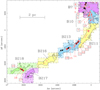 |
Fig. 1 Schematic view of the selected L1495 filament within the Taurus Molecular Cloud Complex (adapted from Hacar et al. 2013). The offsets refer to the centre at α = 4h 17m47.1s, δ = +27°37′18′′ (J2000). Theblack solid line represents the lowest C18O(1–0) contour (0.5 K km s−1). The red linesrepresent the N2H+(1–0) emission (first contour and contour interval are 0.5 K km s−1), which traces the dense cores. The C18O(1–0) and N2H+(1–0) data are from Hacar et al. (2013). The red labels identify the cores found by Hacar et al. (2013), and black squares around the labels show the cores studied in this work. The stars correspond to young stellar objects from the survey of Rebull et al. (2010). Solid symbols represent the youngest objects (Class I and Flat), and open symbols represent evolved objects (Class II and III). |
4 Results
4.1 Distribution of gas emission
Figure 2 presents the spectra of all four species towards the N2H+(1–0) emission peak of each core. For core 4, where the reference position was contaminated with N2H+(1–0) emission, we present the spectra towards the N2D+(2–1) emission peak.
There are starless (2, 3, 4, 6, 7, 8, 10, 12, 16, 17, and 19) and protostellar (11 and 13) cores among the observed targets. The protostellar cores host Class 0–I young stellar objects (YSOs). Two YSOs (Class II and III) are close in projection to but not associated with core 8. Two cores (2 and 7) are isolated from other cores and YSOs, the other cores are clustered in chains with other starless and protostellar cores and YSOs (see Fig. 1). The integrated intensity maps are shown in Fig. A.8. All four species are detected towards all observed cores (with S∕N > 5) except for N2D+(2–1) towards core3 (detected with S∕N ≃ 3).
The N2H+(1–0) and N2D+(2–1) emission peaks usually match within one beam size (cores 2, 6, 7, 8, 10, 11, 13, 17, 19), however in cores 12 and 16 the peaks are offset by one or two beam widths (~30–60′′; see Fig. 3). Often the N2H+(1–0) and N2D+(2–1) emission areas have different shapes; the N2D+(2–1) areas are more compact. Emission peaks of N2H+(1–0) and N2D+(2–1) are associated with a position of a YSO towards the protostellar cores (11 and 13). One core (12) has two N2D+(2–1) emission peaks with the N2H+(1–0) emission peak in between (see cores 10–13 in Fig. A.8). H13CO+(1–0) usually has several emission peaks within one core (3, 4, 6, 8, 10, 12, 17) and avoids the N2D+(2–1) emission peaks (2, 3, 4, 6, 10, 12, 16, 17), which is a sign of possible depletion. Towards the protostellar cores 11 and 13, H13CO+(1–0) and DCO+(2–1) are centrally concentrated and their emission peaks are within a beam size to the YSOs. The DCO+(2–1) emission follows the shape of the N2D+(2–1) emission, but it is more extended (4, 6, 7, 10, 11, 13, 16, 17) and in a few cases avoids N2D+(2–1) (2, 3, 8, 12; see Fig. A.8). Towards the cores 7, 11, and 13 all four species have very similar emission distribution and close peak positions.
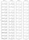 |
Fig. 2 Spectra of all observed transitions towards the N2H+(1–0) intensity peak for each core. The VLSR come from individual fits for each line. For core 4, where the reference position was contaminated with N2H+(1–0) emission, we present the spectra towards the N2D+(2–1) emission peak. The cores with an asterisk (*) near the title contain protostars. |
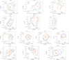 |
Fig. 3 Integrated intensities of the N2D+(2–1), N2H+(1–0), DCO+(2–1), and H13CO+(1–0) lines across the cores. The contours show 60% of the intensity peak; filled circles show the emission peaks. Stars show the positions of YSOs from Rebull et al. (2010): black stars are young, flat, and Class I objects; white stars are more evolved, Class II and III objects. The 27.8′′ beam size of N2H+(1–0) is shown in the bottom left of each panel. |
4.2 Velocity dispersion
The velocity dispersions (σ) of all transitions are determined from the hfs fits. The maps of the velocity dispersions of the N2D+(2–1), N2H+(1–0), DCO+(2–1), and H13CO+(1–0) lines are shown in Fig. A.9. The ranges of the velocity dispersions of the different lines are given in Table 3 with median values (σmedian) and typical uncertainties (Δσ) for easier comparison. The velocity dispersion increases going from higher density gas tracers (N2D+ and N2H+) to lower density gas tracers (DCO+ and H13CO+), as expected(Fuller & Myers 1992). The fact that the N2D+(2–1) velocity dispersion is on average lower than the rest of the lines may be the cause of the observed small velocity centroid shifts (see Sect. 4.4 and Fig. 5). Tracers of the lower density parts of the core may show more material along the line of sight with slightly different velocities than those traced by N2D+ and producethe small shifts (this possibility was shown with simulations in Bailey et al. 2015).
The velocity dispersion increases towards YSOs (cores 3, 8, 11, 12, 13, 17, 19); there is a protostellar core 18 between cores 17 and 19 (see e.g. Fig. 1). Nevertheless, the linewidths stay very narrow across the cores and are dominated by thermal motions (see Sect. 4.3 for details). The N2D+(2–1) velocity dispersions become large (compared to the thermal linewidth) only towards the protostar in core 13 and on the edges of cores 6, 7, and 19. The N2H+(1–0) velocity dispersions become large (compared to the thermal linewidth) only towards the protostars in cores 11 and 13, and on the edges of cores 6, 7, 8, and 16. The N2H+(1–0) and H13CO+(1–0) lines towards cores 3, 8, 13, and 16 also have hints of a second velocity component that is not clearly resolved with our observations, which may increase the velocity dispersions towards those positions (see Sect. A.2 for details). A small fraction of the DCO+(2–1) and H13CO+(1–0) spectra show a transonic velocity dispersions towards each core. The DCO+(2–1) lines show asymmetric, double-, or multiple-peaked lines which are probably unresolved multiple velocity components towards all cores (see Sect. A.2 for details).
Velocity dispersions (σ) of the observed lines.
4.3 Non-thermal motions
Figure 4 shows the ratio of the non-thermal components σNT of the N2D+(2–1), N2H+(1–0), DCO+(2–1), H13CO+(1–0), and C18O(1–0) lines in each pixel of the maps and the thermal velocity dispersion of a mean particle, σT, as a function of core radius measured as a distance from the pixel to the N2H+(1–0) emission peak. The C18O(1–0) velocity dispersions come from the fit results in Hacar et al. (2013). For the C18O(1–0) plot, we take only the CO components whose VLSR coincide with the VLSR of the dense gas. The non-thermal components are derived from the observed velocity dispersion σobs via
 (1)
(1)
where k is Boltzmann’s constant, Tk is the kinetic temperature, and mobs is the mass of the observed molecule. The formula is adopted from Myers et al. (1991), taking into account that σ2 = Δv2∕(8ln(2)), where Δv is the full width at half maximum (FWHM) of the line. To measure the non-thermal component, we use the kinetic temperature determined by Seo et al. (2015) from ammonia observations. We use the same temperature for all five lines, the temperature towards the N2H+(1–0) peak, for each core. The variations in the kinetic temperature across the mapped core areas are within 1–2 K, which produce an uncertainty of 6%–12%in the σNT∕σT ratio. Since the kinetic temperature of the gas in the studied cores usually increases towards their edges, we can expect the right-hand sides of the distributions in Fig. 4 to shift to lower values by 6%–12%.
The thermal velocity dispersions σT for a mean particle with mass 2.33 amu are 0.17–0.21 km s−1 for typical temperatures of 8–12 K across the cores of L1495. The majority of all four high density tracers’ lines are subsonic. However going from tracers of more dense gas to tracers of less dense gas, the fraction of transonic (1 < σNT∕σT < 2) lines increases: 0.8% of the N2D+(2–1) lines, 2.6% of the N2H+(1–0) lines, 19% of the DCO+(2–1) lines, and 24% of the H13CO+(1–0) lines are transonic, while 67% of the C18O(1–0) lines show transonic or supersonic linewidths. One should remember that all considered points are on the line of sight through the cores and ambient cloud (filament), and we consider that all high density tracers belong to dense cores (with H13CO+ also providing a connection to the cloud) and C18O represents mostly the cloud. The median σNT∕σT ratio also increases from high to low density, that is 0.49, 0.58, 0.84, 0.81, and 1.16 for N2D+(2–1), N2H+(1–0), DCO+(2–1), H13CO+(1–0), and C18O(1–0), respectively. The maximum non-thermal to thermal velocity dispersion ratio is 1.4 for N2D+(2–1), 1.5 for N2H+(1–0), 1.6 for DCO+(2–1), 2.4 for H13CO+(1–0), and 3.9 for C18O(1–0). The ratio slightly decreases with radius for N2D+(2–1) and DCO+(2–1), but stays relatively constant for N2H+(1–0) and H13CO+(1–0). The highest density in the points distribution occupies the same σNT∕σT range in the N2H+ and N2D+ plots (0.4–0.6), and another zone for H13CO+ and DCO+ (0.65–0.85). We also estimate the σNT∕σT ratio for the DCO+ lines with well-constrained τ (11% of all data points). The median ratio is 0.55, which is even smaller than the ratio for N2H+. However, eliminating the lines with the unconstrained τ (89% of all data points), we exclude both multiple component lines and optically thin lines, which are present mainly in the core outskirts. Nevertheless, with possibly overestimated velocity dispersions of N2H+(1–0) and H13CO+(1–0) and to a greater extent DCO+(2–1), the lines stay subsonic and split between more narrow N2D+/N2H+ with 0.5 σT and less narrow DCO+/H13CO+ with 0.8 σT.
 |
Fig. 4 Ratio of non-thermal components of N2D+(2–1), N2H+(1–0), DCO+(2–1), H13CO+(1–0), and C18O(1–0) to the thermal linewidth of a mean particle as a function of radius (distance from the N2H+(1–0) intensity peak) for all cores. The solid and dashed blue lines show the ratios equal to 1 and 0.5. The colour scale represents the density of the points. |
4.4 Velocity field: VLSR and velocity gradients
The centroid velocities VLSR of all the transitions are determined from the hfs fits. The maps of the centroid velocities of the N2D+(2–1), N2H+(1–0), DCO+(2–1), and H13CO+(1–0) lines across the cores are presented in Fig. A.10. The range of the VLSR seen in all lines (6.3–7.6 km s−1) is narrower than the velocity range seen across the entire filament in NH3 (5.0–7.2 km s−1; Seo et al. 2015) and C18O (4.5–7.5 km s−1; Hacar et al. 2013), which trace both dense and diffuse gas. The velocity fields traced by the four lines are usually similar within one core. The dense gas in core 13, which hosts the Class 0 protostar IRAS 04166+2706 (Santiago-García et al. 2009), has a peculiar velocity field in that the different species have significantly different velocity field morphologies. It is probably affected by the outflow of the protostar.
Figure 5 presents velocity profiles along the fibre directions defined in Hacar et al. (2013), from core 19 in the south-east to core 8 in the north-west. Some cores (3, 7, 8, 10, 17, and 19) are located next to the places where the fibres change their directions. Core 2 is not associated with any fibre, such that we use a –45° position angle measured from the north to the east for the filament direction there. The velocity changes both along and across the fibres. To better show the difference in velocity between N2H+ and N2D+ we plot data only for these molecules in Fig. A.12. Figure A.12 shows that the N2D+(2–1) velocity is less spread than that of N2H+(1–0) and the other lines towards cores 6, 8, 10, 11, 12, 13, and 16 (all observed cores in more evolved subregions B213 and B7, and core 6).A comparison of the velocity maps in Fig. A.10 shows that the smaller area of the N2D+(2–1) emission cannot explain the difference; the densest gas does not participate in the oscillative distribution of material along the fibres as seen in N2H+ and other tracers. The highest dispersions of the centroid velocities (≃0.6 km s−1) appear at the protostellar cores (11 and 13) and cores close to a protostar (10, 12, 17, and 19).
The VLSR of DCO+(2–1) towards core 7 is systematically lower than that of other tracers. The DCO+(2–1) line is blended with a second velocity component and the VLSR has a systematic shift because of the line asymmetry (see Fig. 2). The N2D+(2–1) velocity along the filament is lower than that of N2H+ and the other species in the majority of data points. The lower VLSR values are associated with the smaller N2D+ velocity dispersion values (compared to those of N2H+), which confirms our suggestion that N2H+ traces more material along the line of sight with possibly different velocities.
 |
Fig. 5 VLSR along the filament direction (from core 19 in the south-east to core 8 in the north-west). The transitions are shown with colours: N2D+(2–1) – red circles; N2H+(1–0) – blue squares; DCO+(2–1) – orange flipped triangles; H13CO+(1–0) – green triangles; and C18O(1–0) – black circles. The vertical bars show the N2H+(1–0) emission peaks. Stars show the positions of YSOs from Rebull et al. (2010): black stars indicate flat and Class I objects, white stars indicate Class II and III objects. |
4.5 Total gradients and specific angular momentum
Assuming that the cores are in solid body rotation, we estimate total and local velocity gradients across the cores following the method described in Goodman et al. (1993) for total gradients and applied for local gradients by Caselli et al. (2002a; see Sect. 4.6 for local gradients). The results of the total velocity gradient calculation provide the average velocity across the core ⟨VLSR⟩, the magnitude of the velocity gradient G, and the position angle θG. The total gradients are calculated using all available points weighted by  , where
  is the uncertainty of the central velocity. We also calculate the specific angular momentum as J∕M ≡ pΩR2, where p = 0.4 is a geometry factor appropriate for spheres, Ω is the angular velocity, derived from the velocity gradient analysis, R is the radius, with the assumption that
  , where S is the emittingarea (see e.g. Phillips 1999), which is the area of the velocity map. Not all the cores are spherical, however we assume spherical geometry to be consistent in our approach to treat all of them. The assumption of sperical geometry introduces a systematic difference by 20% to the resulting specific angular momentum for the elongated cores if we consider the rotation axis parallel to the core axis. The total gradient direction, which in our assumption is a direction of core rotation, is not always parallel to either of the core axes, in fact the angles are random, so we cannot use the same approach (cylinder or disc shape) for all cores. In this situation the best approach is to assume spherical geometry.
4.5.1 Total gradients and specific angular momentum measured over all detected emission
At first, ⟨VLSR⟩, G, θG, R, and J∕M are calculated for all emitting areas for each species (the numbers are given in Table B.1). The total gradients of the four species with their position angles are shown in Fig. B.1. One can expect that higher density tracers have smaller gradient values than lower density tracers, as the decrease in velocity gradient values should trace the loss of the corresponding specific angular momentum towards small scales (Crapsi et al. 2007; Belloche 2013). That means that velocity gradients should increase in a sequence N2D+ → N2H+ → DCO+ → H13CO+. Only core 19 obeys this sequence. Four cores (4, 6, 8, and 16) increase their gradients in a sequence N2D+ → N2H+ → H13CO+ → DCO+, although for core 4 there is no N2H+ data and gradients of DCO+ and H13CO+ differ within the uncertainties by ≃1%. Three cores (11, 12, and 13), belonging to one core chain, increase their gradients in a sequence N2H+ → N2D+ → H13CO+ → DCO+. Core 17 has the sequence N2H+ → N2D+ → DCO+ → H13CO+; core 10 has the sequence N2D+ → H13CO+ → N2H+ → DCO+. Cores 2 and 3 have the sequence H13CO+ → DCO+ → N2H+ → N2D+; core 2 has equal DCO+ and H13CO+ gradients and core 3 has an unreliable detection of N2D+ with S∕N = 3. Core 7 has the sequence DCO+ → H13CO+ → N2H+ → N2D+. The differences between the gradient values are significant taking the errors into account. If we assume that N2H+ and N2D+ equally well trace the dense central part of a core, and DCO+ and H13CO+ equally well trace the more diffuse envelope of a core, we have 10 out of 13 cores that follow the expectations about total gradient increase. There are three cores (2, 3, and 7) that show a total velocity gradient increase towards the denser gas (similar to L1544; Caselli et al. 2002b). Cores 2 and 7 are isolated starless cores, whereas core 3 has an evolved YSO nearby. Among these only core 7 shows a coherent velocity field and very likely is in solid body rotation.
Specific angular momentum varies in a range (0.6–21.0) × 1020 cm2 s−1 with a typical error of (0.02–0.21) × 1020 cm2 s−1 at core radii between 0.019–0.067 pc. It is similar to the results for other dense cores (J∕M = (6.2–30.9) × 1020 cm2 s−1 at radii 0.06–0.60 pc and J∕M = (0.04–25.7) × 1020 cm2 s−1 at radii 0.018–0.095 pc, Goodman et al. 1993; Caselli et al. 2002a, respectively). Figure 6 shows the correlation between specific angular momentum and radius of the core. For each species we find a best-fit power-law correlation aRb: for N2D+(2–1), J∕M = 1023±1R1.8±0.8 cm2 s−1; for N2H+(1–0), J∕M = 1024±1R2.4±0.9 cm2 s−1; for DCO+(2–1), J∕M = 1024±1R2.0±1.1 cm2 s−1; and for H13CO+(1–0), J∕M = 1024±1R2.2±0.7 cm2 s−1. These numbers agree with those found by Goodman et al. (1993) with ammonia observations, that is J∕M = 1022.8±0.2R1.6±0.2 cm2 s−1. We note that the radii used to calculate J∕M in this work are larger than the radii at FWHM of emission. The significant difference between FWHM and equivalent radius of emission (see Fig. B.4) shows that the common approach to use the FWHM as size of a core may not be correct. However if we use FWHM as a size of the core we also see the decrease in the specific angular momentum at higher densities in the majority of the cores (see Table B.4). All data used to calculate J∕M have S∕N > 5 except for the N2D+ data for core 3 with S∕N ≃ 3.
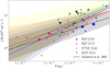 |
Fig. 6 Specific angular momentum as a function of core radius measured with different lines. Large symbols show protostellar cores, small symbols show starless cores. The lines are the best fits of a power-law function aRb calculated for each species (N2H+(1–0) – blue, N2D+(2–1) – red, H13CO+(1–0) – green, DCO+(2–1) – yellow), a and b values are given in the main text. The black line shows the relation found by Goodman et al. (1993). Thick light colour strips represent the accuracies of the fits (N2H+(1–0) – light blue, N2D+(2–1) – light red, H13CO+(1–0) – light green, DCO+(2–1) – light yellow, Goodman et al. 1993 – grey). |
4.5.2 Total gradients and specific angular momentum measured over the maps with uniform area and resolution
To compare the total velocity gradients for the four species on the same size scale, we convolve all maps to the spatial resolution of 29.9′′, corresponding to the H13CO+(1–0) beam size, with Nyquist grid spacing, and we use only the area where the emission in all four species is detected, which matches where N2D+(2–1) is detected, because this area has the most compact emission. The results of the gradient calculations are given in Table B.2.
We compare the results for N2D+(2–1) with the results obtained with the other species in Fig. B.2. The average centroid velocity ⟨VLSR⟩ of N2D+(2–1) agrees with the ⟨VLSR⟩ of the other species within 1.5%, however for most of the cores the N2D+(2–1) velocity is systematically lower (see Fig. B.2a). The total centroid velocity gradient G of N2D+(2–1) for the majority of cores is also lower than G measured with other species. The range of the total gradients seen in all species is 0.66–7.35 km s−1 pc−1 with the errors in a range 0.02–0.14 km s−1 pc−1. The N2D+(2–1) line is most similar to the N2H+(1–0) line; the maximum difference is 1.9 km s−1pc−1 at core 8 and the median difference being 0.5 km s−1pc−1. The difference with H13CO+(1–0) and DCO+(2–1) is more significant. The maximum difference between N2D+(2–1) and H13CO+(1–0) is 2.8 km s−1 pc−1 at core 16. The median difference is 1.1 km s−1 pc−1. The maximum difference between N2D+(2–1) and DCO+(2–1) is 3.8 km s−1 pc−1 at core 16. The median difference is 1.2 km s−1 pc−1.
The directions of the gradients seen in different species are generally in better agreement. The typical errors of the determination of the position angle are 0.4–3.0°. The best agreement is between N2D+(2–1) and DCO+(2–1); the biggest difference is 94° at core 16, and the median difference is 10°. The biggest difference between N2D+(2–1) and H13CO+(1–0) is 118° at core 16, and the median difference is 11°. The biggest difference between N2D+(2–1) and N2H+(1–0) is 68° at core 16, and the median difference is 12°. Thus, the median difference in the total gradient directions between the species is the same within the uncertainties.
The specific angular momentum varies in a range of (0.7–12.2) × 1020 cm2 s−1 with a typical error of (0.02–0.31) × 1020 cm2 s−1. The J∕M measured in N2D+(2–1) agrees better with the J∕M measured in N2H+(1–0); the median difference is 14% and the maximum difference is 114% at core 8. The J∕M measured in N2D+(2–1) is systematically lower than the J∕M measured in H13CO+(1–0) and DCO+(2–1) (median differences with N2D+(2–1) are 40 and 39%, maximum differences 425 and 578% at core 16) with the exception of core 7.
We also compare the results for DCO+(2–1) and H13CO+ (1–0) in Fig. B.3. The average centroid velocities of the two lines agree within 0.7%. The total centroid velocity gradient of the two species stays along the one-to-one correlation with no systematic difference. A median scatter of G is 0.9 km s−1 pc−1 and the maximum difference is 3.6 km s−1 pc−1 at core 3. The directions of the gradients of DCO+(2–1) and H13CO+(1–0) are in goodagreement, with the difference in position angle varying from 0.4–24° and having a median difference of 6°. The specific angular momentum of the two lines agrees within (0.03–2.2) × 1020 cm2 s−1 with a maximum difference at core 8.
4.6 Local gradients
The local velocity gradients are presented in Fig. B.5 with black arrows plotted over integrated intensity colour maps of the corresponding molecular transition along with red arrows, which present local velocity gradients of C18O(1–0) calculated from the Hacar et al. (2013) fit results (a comparison with the C18O local velocity gradients is given in Sect. 5.2). The maps are convolved to a 29.9′′ beam with Nyquist sampling. To calculate a gradient in a local position, we use all pixels closer than two pixel size distance, weighted according to their distance to the given position and their uncertainty of the central velocity, as follows:
![Mathematical equation: \begin{equation*} W=\frac{1}{{\rm{\Delta}}_{\textrm{V}_{\textrm{LSR}}}^2}\times\exp\left\lbrace-d^2\big/\left[2\left(\frac{\theta_{Gauss}}{2.354}\right)^2\right]\right\rbrace, \end{equation*}](/articles/aa/full_html/2018/09/aa31159-17/aa31159-17-eq8.png) (2)
(2)
where W is the weight,  is the uncertainty of the central velocity, d is the distance from the weighted pixel to the given position, and θGauss = 2 is the FWHM of the weighting function.
Cores 2, 4, and 16 increase their velocities towards the core centres, while core 17 shows velocities decreasing towards the core centre; the arrows shown in Fig. B.5 point towards higher VLSR. For a given core, the velocity fields of the different species are typically fairly similar.
There are, however, some variations from one species to the other, in particular towards theprotostellar cores. Core 13 has the most complex velocity field with the N2H+(1–0) data showing four different velocity gradient directions in various areas across the core. Only two of these gradients can be seen in the N2D+(2–1) data because of the smaller detected extent of the N2D+(2–1) emission. The significant change of the gradient direction on a small spatial scale, which is also present in core 11 and less prominent in cores 3, 8, and 12, is characteristic for a protostellar core, which was first revealed by Crapsi et al. (2004) towards another Taurus core, L1521F. This would imply that the last three cores known as starless may be relatively highly evolved. The difference between N2D+/N2H+ and DCO+/H13CO+ can represent some differential gas motions between the core envelope and central regions.
5 Discussion
5.1 Velocity dispersions
Pineda et al. (2010) defined the coherent dense core as a region with nearly constant subsonic non-thermal motions. The linewidth distribution we see in the dense gas tracers, N2D+(2–1) and N2H+(1–0), shows constant subsonic (≃σT∕2) non-thermal motions (see Fig. 4), in which N2D+ has ≃20% lower non-thermal components than N2H+; this is consistent with these observations tracing the coherent centres of dense cores in L1495.
Pineda et al. (2010) observed a sharp transition to coherence, where the linewidths of NH3(1,1) increased by a factor of at least two over a distance of less then 0.04 pc, which corresponds to their beam size. We do not see any reliable sign of the transition to coherence in any of the tracers that we have observed. One can explain this by the fact that the N2D+(2–1) line, which traces the high density gas, has a significantly higher critical density than the inversion transitions of NH3. Thus, the N2D+ line intensity drops faster towards the edge of the core because the excitation temperature decreases more rapidly than that of the NH3 inversion line. Similarly, for most of the cores, the next highest density gas tracers, the N2H+(1–0) and DCO+(2–1) lines (both having critical densities higher than that of NH3(1,1)), are detected over larger areas and still do not show any sudden increase in linewidth, as seen in NH3. Towards those cores where the emission strongly decreases away from the core centres (cores 6 and 17 for N2H+ and cores 8, 11, 13, 16, and 17 for DCO+), the linewidths at the edges do not increase significantly, or even decrease, from the linewidths towards the centre of the cores. However, even the NH3 maps by Seo et al. (2015), which cover larger areas than our maps, still do not show a significant increase in the velocity dispersions towards the core edges.
We see however supersonic linewidths in H13CO+, where the linewidths reach 2.4 σT in some places. Its transonic non-thermal motions lie mostly between 1 and 1.5 σT, which is consistent with the typical observed C18O non-thermal component (see Fig. 4). H13CO+ tends to be slightly (cores 2, 6, 8, 10) or significantly (cores 4, 12, 16) depleted towards the core centres and better traces the core envelopes compared to N2D+ and N2H+. The fact that the median velocity dispersions of N2D+(2–1) and the N2H+(1–0) are 1.3–1.6 times lower than the median velocity dispersions of DCO+(2–1) and H13CO+(1–0) indicates that the velocity dispersion is indeed increasing outwards.
5.2 Connection to the filament scale
To search for a connection from the cores and their envelopes to the filament scale, we estimate local and total VLSR gradients of the CO and compare the velocity field patterns and total gradients to the patterns seen in each species we observed. For the CO data we use the fit results of the C18O(1–0) mapping carried out by Hacar et al. (2013), which created maps convolved to a 60′′ beam size. In their work, Hacar et al. (2013) found multiple velocity components of the C18O(1–0) line and revealed the fibre structure of the L1495 filament. These authors classified the fibres as “fertile”, if they host dense cores and coincide with N2H+ emission, and “sterile” if they do not. For our study, we take only the C18O(1–0) components that have a VLSR close to the VLSR of our lines (6.3–7.6 km s−1).
We show the maps of local velocity gradients in Fig. B.5. In this figure, black arrows represent the velocity gradients of N2D+(2–1), N2H+(1–0), DCO+(2–1), and H13CO+(1–0) and red arrows represent the velocity gradients of C18O(1–0). For the majority of the cores, the C18O velocity gradient value G is lower than the G of the other lines. The velocity field of the dense gas is affected by protostars both in protostellar cores (11 and 13 as seen in all species) and cores sitting next to protostellar cores and YSOs (3, 8, 10, 12, 16, 17, and 19 as seen mostly in H13CO+; see Sect. 4.6). While the C18O velocity fields do not show the same level of complexity as that of the dense gas tracers, the velocity field of the C18O is by no means uniform and exhibits changes in direction in cores 3, 8, 10, 16, and 19.
In cores 3, 6, 12, and 19 the velocity pattern of C18O matches the patterns of the higher density tracers, and the agreement is better between C18O, N2H+, and N2D+. In cores 4, 11, 13, and 17, C18O has uniform velocity patterns that match some velocity patterns seen in N2H+, DCO+, and H13CO+. In the northern half of core 8 the velocity pattern of C18O matches the velocity patterns of N2D+, DCO+, and H13CO+ (the velocity increases to the north-west) while in the southern half of the core the C18O velocity gradient is perpendicular to the gradients of the other species. In the southern half of core 8, the dense gas tracers all increase in velocity towards the south-west, towards a YSO, whereas the CO velocity increases to the north-west. In core 16 the velocity of the high density tracers increases towards the core centre and the velocity of the C18O increases towards a position ~1′ to the northof the core, so the pattern looks similar but shifted, although this could be insignificant given the 60′′ beam size of the C18O data. In core 2 the velocity of the high density tracers also increases towards the core centre and the velocity of the C18O uniformly increases towards the south-west of the core. Core 10 has curved velocity fields both in the C18O and high density tracers, although the C18O velocity field is roughly perpendicular to the velocity fields of the other tracers towards most locations. Core 7 has coherent velocity fields both in C18O and high density tracers (local gradients arrows almost parallel in C18O and divergent in the other species), orientated with an angle to each other that changes from 90° to 0°. In general, C18O show similar velocity patterns in the starless cores as high density tracers with less complexity. C18O does not show any affect from embedded protostars in the protostellar cores, which makes the C18O velocity gradients almost perpendicular to those of the high density tracers.
The total gradients are shown in Fig. B.1. The difference between C18O and the higher density tracers is more significant in the overall gradient directions because of the additional complexity of the higher density tracers’ velocity fields. Cores 4 and 6 show a good correlation between C18O and the other species; the largest difference is the 8° separation between the C18O and H13CO+ gradients in core 6. Cores 3, 6, 7, 8, 10, 11, 12, 17, and 19 show directions for the gradient of C18O, which differ less than 90° (20°–83°) from that of the dense gas tracers. The C18O gradient differs by more than 90° from that of at least one dense gas tracer in cores 2, 13, and 16, although the total velocity gradient of C18O towards core 2 has a large error of 40° owing to the small number of data points. Core 13 has very complex velocity fields of the higher density tracers due to the strong effect of the embedded protostar. Core 16 has complex velocity patterns both in C18O and the higher density tracers, which affect the total gradient. For the majority of the cores, the C18O(1–0) velocity field coincides with those of the high density tracers but does not show the variations near YSOs (cores 8, 11, 12, 13, 17, and 19) that are seen in high density tracers.
The value of the C18O total velocity gradient (0.3–3.3 km s pc−1 measured with a typical error of 0.03–0.17 km s pc−1) is usually lower than that of the other species (0.6–6.1 km s pc−1 in cores 2, 3, 6, 7, 8, 10, 13, and 16) or lower than that of only DCO+ and H13CO+ (cores 4, 11,12, 17, and 19). This may mean that the denser material is spinning up in the process of core formation.
5.3 Velocity gradient and large-scale polarization
Caselli et al. (2002b) found that in another Taurus core, L1544, the directions of the total gradients observed in DCO+(2–1) and N2H+(1–0) are similar to the direction of the magnetic field. In Fig. 7 we compare the total velocity gradients of our N2D+(2–1), N2H+(1–0), DCO+(2–1), and H13CO+(1–0) maps and C18O(1–0) from Hacar et al. (2013) with the polarization directions measured with optical (Heyer et al. 1987) and infrared (Goodman et al. 1992; Chapman et al. 2011) observations. The magnetic field is parallel to the polarization direction. Chapman et al. (2011) pointed out that where the filament turns sharply to the north (above core 7 or starting from the B10 subregion and farther up in Fig. 1), the magnetic field changes sharply from being perpendicular to the filament to being parallel to the filament.
To quantify the alignment of the total velocity gradients with the polarization directions, we plot the minimum angle between the corresponding position angles (see left panel of Fig. 8). In Fig. 8 the grey and cyan strips show the directions within 10° of being parallel or perpendicular to the magnetic field, respectively, because the typical uncertainty of the position angle difference is of the order of 10°. There is not a big difference between the species in the alignment and the polarization directions. We compare the alignment of the polarization directions with a random angle distribution (see right panel of Fig. 8). The alignment between the total velocity gradient and polarization directions is comparable to a random distribution: 27% of the gradient directions are parallel to the polarization directions and 14% of the random directions are parallel to the polarization directions; 13% of the gradient directions are perpendicular to the polarization directions and 14% of the random directions are perpendicular to the polarization directions.
We also compare the gradient directions with the directions of the fibres that host the cores and test if the alignment is significant compared to a random distribution of the angles (see Fig. 9). The alignment between the total gradient directions and the directions of the fibres is comparable to a random distribution: 10% of the gradient directions are parallel to the directions of the fibres and 10% of the random directions are parallel to the directions of the fibres; 7% of the gradient directions are perpendicular to the directions of the fibres and 8% of the random directions are perpendicular to the directions of the fibres. Figure 10 compares cumulative distributions of the angles between the total gradients, polarization, fibre directions, and random directions.
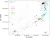 |
Fig. 7 Polarization in L1495 measured with optical (Heyer et al. 1987; grey segments) and infrared (Goodman et al. 1992; Chapman et al. 2011) observations (cyan segments) and total velocity gradients across the cores (N2D+ – red, N2H+ – blue, DCO+ – orange, H13CO+ – green, and C18O – black). The colour scale shows the dust continuum emission at 500 μm obtained with Herschel/SPIRE (Palmeirim et al. 2013). |
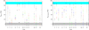 |
Fig. 8 Left panel: difference between polarization angles θpol and position angles of the total gradients θG for each core (N2D+ – red circles, N2H+ – blue squares, DCO+ – orange flipped triangles, H13CO+ – green triangles, and C18O – black diamonds). Right panel: difference between θpol and a set of random angles θrandom from 0 to 90°. Grey strip corresponds to parallel directions ± 10°; cyan strip corresponds to perpendicular directions ± 10°. |
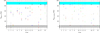 |
Fig. 9 Left panel: difference between fibre position angles θfibre and position angles of the total gradients θG for each core (N2D+ – red circles, N2H+ – blue squares, DCO+ – orange flipped triangles, H13CO+ – green triangles, and C18O – black diamonds). Right panel: difference between θfibre and a set of random angles θrandom from 0 to 90°. Grey strip corresponds to parallel directions ± 10°; cyan strip corresponds to perpendicular directions ± 10°. |
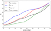 |
Fig. 10 Cumulative distribution of angles between the random angles and polarization (red), total gradients and polarization (blue), total gradients and fibre directions (green), and random angles and fibre directions (black). |
5.4 Dynamical state of the cores
Six out of 13 cores (6, 7, 8, 10, 12, and 19, all starless) show relatively coherent velocity fields that are consistent with solid body rotation. Five of the listed above cores show significantly lower total gradients in higher density tracers (N2D+ and N2H+) than in lower density tracers (DCO+ and H13CO+) on a core scale, which implies that denser material is spinning down. This does not contradict the fact that all four core tracers show higher total velocity gradients than C18O. At the levelof cloud-core transition, the core material, namely its external envelope traced by DCO+ and H13CO+, is spinning up, which is consistent with conservation of specific angular momentum. However, within the core at higher densities the central material traced by N2D+ and N2H+ is spinning down. The decrease in specific angular momentum with density may be caused by such mechanisms as magnetic braking, gravitational torques, and the transfer of angular momentum into the orbital motions of fragments if further material fragmentation takes place in the cores as explained by Belloche (2013). However our current data do not allow us to investigate the possible fragmentation and dynamics of the material within the cores at smaller scales because of the limited angular resolution. These five cores may be more evolved than the other cores not listed here. Three starless cores (3, 8, and 12) show complex local velocity gradient patterns resembling those of protostellar cores, thus they may contain a very low luminosity object, as in the case of L1521F (Crapsi et al. 2004; Bourke et al. 2006).
Emission peaks of N2H+(1–0) and N2D+(2–1) are associated with the position of a YSO towards both protostellar cores, 11 and 13. This means that these YSOs are very young or very low luminosity, such that they have not yet affected the chemistry of their surrounding. One core (12) has two N2D+(2–1) emission peaks with the N2H+(1–0) emission peak in between (see Fig. A.8), which could be a sign of further core fragmentation or binary formation.
Four cores (6, 7, 12, and 17) show that the N2D+(2–1) emission is more elongated and compact than the emission from the other lines. This may mean that the N2D+ is tracing the higher density gas, which may be contracting along the magnetic field lines, thus producing the elongated structure.
6 Conclusions
This paper presents maps of four high density tracers, N2D+(2–1), N2H+(1–0), DCO+(2–1), and H13CO+(1–0), towards 13 dense cores (starless and protostellar) along the L1495 filament. We use N2D+(2–1) and N2H+(1–0) as tracers of the core central regions, and DCO+(2–1) and H13CO+(1–0) as tracers of the core envelope. We measure velocity dispersions, local and total velocity gradients, and specific angular momenta. We connect the core-scale kinematics traced by these high density tracers to the filament-scale kinematics traced by the C18O(1–0) observations presented in Hacar et al. (2013). We study the variations in the dense gas kinematics along the filament. Our main findings are as follows:
All studied cores show similar kinematic properties along the 10 pc-long filament. These cores have similar central velocities (6.3–7.6 km s−1), similar velocity dispersions (mostly subsonic), the same order of total velocity gradient magnitudes (0.6–6 km s pc−1), and the same order of specific angular momentum magnitudes (~1020 cm2 s−1). This is consistent with the overall coherent structure of the whole filament (Hacar et al. 2013).
N2D+(2–1) shows the most centrally concentrated structure, followed by N2H+(1–0), DCO+(2–1), and H13CO+(1–0), which is consistent with chemical models of centrally concentrated dense cores with a large amount of CO freeze-out onto dust grains.
The cores show very uniform velocity dispersions. The N2D+(2–1) and N2H+(1–0) lines are subsonic, close to 0.5 σT with thermal linewidth σT = 0.17–0.21 km s−1. The DCO+(2–1) and H13CO+(1–0) lines are mostly subsonic, close to 0.8 σT, and partly transonic. The non-thermal contribution to the velocity dispersion increases from higher to lower density tracers. The median σNT∕σT are 0.49, 0.58, 0.84, 0.81, and 1.16 for N2D+(2–1), N2H+(1–0), DCO+(2–1), H13CO+(1–0), and C18O(1–0), respectively. The non-thermal contribution increases by ≃20% from N2D+ to N2H+, and by ≃40% from N2H+ to DCO+ and H13CO+ and further to C18O.
The total velocity gradients of the observed core tracers show a variety of directions and values. For 10 out of 13 cores the higher density tracers N2D+(2–1) and N2H+(1–0) show lower gradients than the lower density tracers DCO+(2–1) and H13CO+(1–0), implying a loss of specific angular momentum at small scales owing to magnetic braking, gravitational torques, and/ or the transfer of angular momentum into the orbital motions of fragments, as theoretically expected (e.g. Belloche 2013). The other 3 cores present different behaviour: core 7, the most isolated and located at the position where the magnetic field changes direction, presents a higher gradient in the higher density tracers; and cores 2 and 3 present a complex kinematic field both in the low and high density tracers, which prevents a meaningful determination of the total velocity gradient. The change of magnitude and direction of the total velocity gradients depending on the tracer indicates that internal motions change at different depths within the cloud.
The above point is strengthened by looking at local velocity gradients, which show complex patterns, especially in comparison with the velocity field traced by C18O (although with lower spatial resolution). Half of the cores (6 out of 13) show a velocity pattern that is consistent with solid body rotation. The velocity fields are mainly similar in different high density tracers, however DCO+(2–1) and H13CO+(1–0) show more local variations because they also trace some of the additional motions within the extended core envelope. The presence of a YSO at a distance less than 0.1 pc from a core locally affects the velocity field of the core.
C18O traces the more extended cloud material whose kinematics is not affected by the presence of dense cores: its total velocity gradient is always lower than that of DCO+ and H13CO+, the core envelope tracers. For the majority of the cores, the C18O velocity field coincides with that of the high density tracers, but does not show the variations near YSOs (cores 8, 11, 12, 13, 17, and 19) seen in the high density tracers, thus suggesting that the gas traced by C18O is not affected by protostellar feedback. At the level of cloud-core transition, the external envelope of the core traced by DCO+ and H13CO+ is spinning up, which is consistent with conservation of angular momentum during core contraction.
The specific angular momenta of the cores vary in the range (0.6–21.0) × 1020 cm2 s−1, which is consistent with previous observations of dense cores (Goodman et al. 1993; Caselli et al. 2002a). The specific angular momentum decreases at higher densities, which shows the importance of local magnetic fields to the small scale (central ≃0.02 − 0.06 pc) dynamics of the cores.
The distributions of angles between the total velocity gradient and the large-scale magnetic field and the distributions of angles between the velocity gradient and filament direction are consistent with being random. This suggests that the large-scale magnetic fields traced by optical and near-infrared polarization measurements is not important in shaping the high density regions of the filament.
Further studies with higher spatial and spectral resolution are needed to understand if local magnetic fields affect possible further fragmentation of the cores and if the latter also cause the decrease in specific angular momentum in their central parts.
Acknowledgements
The authors thank the anonymous referee for valuable comments that helped improve the manuscript. AP thanks Anton Vasyunin for useful comments. The authors acknowledge the financial support of the European Research Council (ERC; project PALs 320620); Andy Pon acknowledges that partial salary support was provided by a CITA National Fellowship. This work ispart of the research programme VENI with project number 639.041.644, which is financed by the Netherlands Organisation for Scientific Research (NWO). MT and AH thank the Spanish MINECO for support under grant AYA2016-79006-P.
Appendix A Line fitting
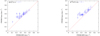 |
Fig. A.1 Comparison of linewidths (FWHM) obtained with Gaussian and hfs fits towards core 11 for DCO+(2–1) (left panel) and for H13CO+(1–0) (right panel). The red lines show one-to-one correlation. |
A.1 Comparison of hyperfine splitting and Gaussian fit results for the H13CO+(1–0) and DCO+(2–1) transitions
We compare the linewidths obtained by fitting the H13CO+(1–0) and DCO+(2–1) line with single Gaussians and taking into account the hyperfine structure (hfs). We find that the Gaussian method gives systematically larger linewidths than the hfs method. The hfs of the H13CO+ and DCO+ rotational transitions were previously studied by Schmid-Burgk et al. (2004) and Caselli & Dore (2005). However the impact of hyperfine splitting in the DCO+ transitions higher than the (1–0) transition and in H13CO+ was assumed negligible (e.g. Volgenau et al. 2006; Hirota & Yamamoto 2006). We implemented hfs fits of the H13CO+(1–0) and DCO+(2–1) transitions in Pyspeckit. The linewidths calculated with the hfs fits are systematically smaller than with the Gaussian fit. For this comparison, we use all of the spectra towards core 11 that have a S∕N > 5, produce fits that give uncertainties to the derived linewidth under 10%, and for which there is no sign of any asymmetry or multiple peaks. On average, the Gaussian linewidths are 25% wider than the hfs derived linewidths for H13CO+(1–0) and 22% wider for DCO+(2–1) (see Fig. A.1).
A.2 Multiple velocity components and self-absorption
All spectra were fitted assuming one velocity component. To check the fit quality, we inspected by eye any spectrum for which the residual after fitting divided by rms was less than 0.8 or more than 1.2. Ratio less than 0.8 implies an overfit when routine fits the noise features instead of the spectral line. A ratio higher than 1.2 implies the fit does not reproduce the line correctly. A significant difference between the data and the fit could be due to the presence of a second line component, self-absorption of the line, asymmetric wings caused by gas flows, or non-LTE effects. The N2D+(2–1) fits do not show significant differences between the fits and the data. The N2H+(1–0) and H13CO+(1–0) spectra show the presence of a second component towards cores 3, 8, 13, and 16 (see Figs. 2 and A.5). The DCO+(2–1) spectra show double-peaked lines caused by either multiple velocity components or self-absorption towards all cores. Many N2H+(1–0) spectra also show non-LTE effects in the intensities of the hfs components, similar to those described in Caselli et al. (1995). Since the non-LTE effects do not affect the velocity dispersion and central velocity estimates, they are not taken into account in this work.
N2H+, DCO+, and H13CO+ show the same line asymmetries, blue and red wings, towards cores 2, 6, 7, 10, 11, 13, and 19 (see Fig. A.5). The asymmetries also appear in the lines of the rare isotopologues D13CO+ and HC18O+ towards cores 2, 4, 7, 10, and 13 (see Fig. A.6). The wings cause an increase of the velocity dispersion. For example, on the north edge of core 10 the isolated component of the N2H+(1–0) hfs traces a gas flow that appears to connect the core and the envelope (see Fig. A.3). The other observed tracers also show an increase of the linewidth at the same place towards core 10 (see Fig. A.9).
DCO+(2–1) and H13CO+(1–0) have no isolated components in their hfs. Because of the hyperfine components are close, it is not easy to find an unambiguous τ-unconstrained fit with the hfs fitting method, and the Gaussian fits do not properly fit the wings of the lines, thereby producing larger linewidths. If the hfs structure makes the line asymmetric, the VLSR of the Gaussian fit is also altered from the correct value (see Figs. A.1 and A.4). Thus in the case of asymmetric or double-peaked lines in DCO+ and H13CO+ we used a τ-constrained fit (τ = 0.1) to gauge the central velocities. The velocity dispersions produced by the τ-constrained fit of the self-absorbed or blended lines are overestimated, as the fit considers one velocity component and the line is assumed to be optically thin (τ = 0.1). We note that the assumption of the τ-constrained fit overestimates the majority of the velocity dispersion measurements for our DCO+ data. We compared the velocity dispersion values obtained with τ-constrained and τ-unconstrained fits where the optical depth is defined with τ > 3Δτ. The τ-constrained fit produces a velocity dispersion 1–3.3 times larger than the τ-unconstrained fit and has an average dispersion that is 1.56 times larger.
Since DCO+(2–1) and H13CO+(1–0) have no isolated components, it is not possible to distinguish between self-absorbed lines and blended second velocity components. However, we control whether the flux was lost owing to the self-absorption of the lines by observing transitions of the rare isotopologues D13CO+(2–1) and HC18O+(1–0) towards the DCO+(2–1) emission peaks in nine cores; the DCO+(2–1) emission peak would suffer self-absorption more than H13CO+ because of its higher critical densities and because it is more abundant in dense, CO depleted gas. We compare the estimates of the column densities (Ncol) of DCO+ and HCO+ obtained with the rearer isotopologues in Fig. A.7. To estimate the column densities, we assume that both lines are optically thin and the fractional abundances of O and C in the species are the same as the fractional abundances of the elements, 16 O/18O = 560 ± 25, 12C/13C = 77 ± 7 (Wilson & Rood 1994). The comparison shows that both DCO+(2–1) and H13CO+(1–0) do not suffer significant self-absorption. Thus the double-peaked lines are most likely two-blended velocity components that trace different layers of an envelope and need better sensitivity and spectral resolution to be resolved.
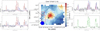 |
Fig. A.2 Integrated intensity map of N2H+(1–0) towards core 13. The red boxes in the map show the areas where the additional velocity components are present. Left panel: the second velocity component (blue fit) is well separated (by ≃1 km s−1) from the main velocity component (red fit). Right top panel: the second velocity component (red fit)is partially blended with the main velocity component (blue fit, the separation is ≃0.3 km s−1 which corresponds to a linewidth σ = 0.13 km s−1). Bottom right panel shows an example spectrum in which only one velocity component is detected with the best fit shown as the greenline. |
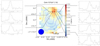 |
Fig. A.3 Velocity dispersion map of N2H+(1–0) towards core 10 with a sample of the gas flow on the edge of the core connecting it to the envelope and the isolated components spectra. |
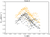 |
Fig. A.4 Comparison of the central velocity (VLSR) of the DCO+(2–1) line measured with Gaussian (yellow) and hfs (black) fits for core 2 plotted along the filament direction. |
We consider that a line has two velocity components if the components are separated by more than one linewidth (such as in core 13, see Fig. A.2). Multiple velocity components are only detected towards an area roughly the size of one to two beams towards core 13. The second components, which are well separated from the main line (see Fig. A.2, left), were missed by the one-component fit procedure and were not taken into account in this work. We tried to avoid the blended components, however, in case they are close (see Fig. A.2, right top) they were fit as one velocity component, which increased velocity dispersion in those points.
A.3 Results of hyperfine splitting fits
Results of a Gaussian fit of D13CO+(2–1) towards the DCO+(2–1) emission peaks of the cores.
Results of an hfs fit of HC18O+(1–0) towards the DCO+(2–1) emission peaks of the cores.
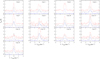 |
Fig. A.5 Spectra of the isolated components of N2H+(1–0) (black), DCO+(2–1) (red), and H13CO+(1–0) (blue) towards the N2H+(1–0) emission peaks. For convenient comparison, the DCO+(2–1) spectra are shifted up by 1 K and the N2H+(1–0) spectra are shifted up by 0.5 K. The cores with an asterisk (*) near the title contain embedded protostrars. |
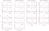 |
Fig. A.6 Spectra of DCO+(2–1) and H13CO+(1–0) (black) compared to D13CO+(2–1) and HC18O+(1–0) respectively towards the DCO+(2–1) emission peaks. For convenient comparison the DCO+(2–1) spectra are divided by 10 and the H13CO+(1–0) spectra are divided by 5. The cores with an asterisk (*) near the title contain embedded protostrars. |
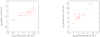 |
Fig. A.7 Comparison of the column densities of DCO+ (left panel) and HCO+ (right panel)towards the DCO+(2–1) emission peaks obtained with an assumption of optically thin lines. The dotted lines show one-to-one correlations. |
Characteristics of the N2H+(1–0), N2D+(2–1), H13CO+(1–0), and DCO+(2–1) maps convolved to 27.8′′, 27.8′′, 29.9′′, and 18′′ beams, respectively.
Characteristics of the N2H+(1–0), N2D+(2–1), H13CO+(1–0), and DCO+(2–1) maps convolved to a 29.9′′ beam.
 |
Fig. A.8 Integrated intensities of the N2D+(2–1), N2H+(1–0), DCO+(2–1), and H13CO+(1–0) lines across the cores. First contour is at the 5σ level and thecontour step is 5σ. Stars show the positions of YSOs from Rebull et al. (2010): black stars indicate young, flat, and Class I objects; white stars indicate more evolved, Class II and III objects. |
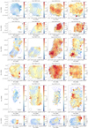 |
Fig. A.9 Velocity dispersions (σ) of the N2D+(2–1), N2H+(1–0), DCO+(2–1), and H13CO+(1–0) lines across the cores. Blue contours show the integrated intensities of the corresponding species. The first contour is at the 5σ level and thecontour step is 5σ. Stars show the positions of YSOs from Rebull et al. (2010): black stars indicate young, flat, and Class I objects, white stars indicate more evolved, Class II and III objects. |
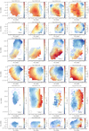 |
Fig. A.10 Central velocities (VLSR) of the N2D+(2–1), N2H+(1–0), DCO+(2–1), and H13CO+(1–0) lines across the cores. Blue contours show the integrated intensities of the corresponding species. First contour is at the 5σ level and thecontour step is 5σ. Stars show the positions of YSOs from Rebull et al. (2010): black stars indicate young, flat, and Class I objects, white stars indicate more evolved, Class II and III objects. |
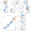 |
Fig. A.11 Opacities of the N2D+(2–1) and N2H+(1–0) lines across the cores. We show only the maps that have more than three pixels with τ-unconstrained fit. Blue contours show the integrated intensities of the corresponding species. First contour is at the 5σ level and thecontour step is 5σ. Stars show the positions of YSOs from Rebull et al. (2010): black stars indicate young, flat, and Class I objects, white stars indicate more evolved, Class II and III objects. |
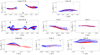 |
Fig. A.12 VLSR along the filament direction (from core 19 in the south-east to core 8 in the north-west). The transitions are shown with colours: N2D+(2–1) – red circles and N2H+(1–0) – blue squares. The vertical bars show the N2H+(1–0) emission peaks. Stars show the positions of YSOs from Rebull et al. (2010): black stars indicate flat and Class I objects, white stars indicate Class II and III objects. |
Appendix B Results of velocity gradients and specific angular momentum calculations
Total velocity gradients G, position angles θG (measured west to north), equivalent radiia measured across the cores using all emitting areas of each species and corresponding specific angular momenta J∕M.
Total velocity gradients G, position angles θG (measured west to north), equivalent radiia, measured across the cores maps convolved to the largest beam of 29.9′′ using the emitting area of N2D+(2–1) and corresponding specific angular momenta J∕M.
Parameters of 2D Gaussians fitted to the N2D+(2–1) integrated intensity maps: centres of the ellipses, major and minor axes, position angles, and aspect ratios.
Total velocity gradients G and FWHM radii RFWHM measured across the cores maps convolved to the largest beam of 29.9′′. The RFWHM are calculatedusing the N2D+(2–1) maps that trace the densest gasa.
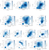 |
Fig. B.1 Total velocity gradients of the N2D+(2–1) (red), N2H+(1–0) (blue), DCO+(2–1) (orange), H13CO+(1–0) (green), and C18O(1–0) (black) lines across the cores. The colour scale shows the integrated intensities of N2D+(2–1) across the cores except core 3, where the integrated intensity of N2H+(1–0) is shown. The ellipses show the 2D Gaussian FWHM fitted to the N2D+(2–1) integrated intensity maps (N2H+(1–0) for core 3). Stars show the positions of YSOs from Rebull et al. (2010): black stars indicate young, flat and Class I objects, white stars indicate more evolved, Class II and III objects. |
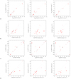 |
Fig. B.2 N2D+(2–1) compared to N2H+(1–0), H13CO+(1–0), and DCO+(2–1): a) average velocity across the core; b) total velocity gradient; c) position angle of the total velocity gradient; and d) specific angular momentum. Open circles show starless cores and filled circles show protostellar cores. For the comparison, all maps are convolved to the largest beam of 29.9′′ with Nyquist spacing and only the area that contains N2D+(2–1) emission is used. |
 |
Fig. B.3 DCO+(2–1) compared to H13CO+(1–0): a) average velocity across the core; b) total velocity gradient; c) position angle of the total velocity gradient; d) specific angular momentum. Open circles show starless cores and filled circles show protostellar cores. For the comparison, all maps are convolved to the largest beam of 29.9′′ with Nyquist spacing and only the area that contains both H13CO+(1–0) and DCO+(2–1) emission is used. |
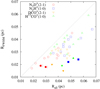 |
Fig. B.4 Core radius at FWHM of maximum emission vs. the radius of the total emitting area measured with different species. Filled symbols show protostellar cores, and open symbols show starless cores. The dashed line shows a one-to-one correlation. |
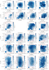 |
Fig. B.5 VLSR local gradients of the N2D+(2–1), N2H+(1–0), DCO+(2–1), and H13CO+(1–0) lines across the cores (black arrows) and VLSR local gradients of the C18O(1–0) line from Hacar et al. (2013; red arrows). The scale of the C18O(1–0) gradients is 2.5 times larger than the scale indicated in the figures. The colour scale shows integrated intensities of corresponding species across the cores. Stars show the positions of YSOs from Rebull et al. (2010): black stars indicate young, flat and Class I objects, white stars indicate more evolved, Class II and III objects. |
References
- André, P., Di Francesco, J., Ward-Thompson, D., et al. 2014, Protostars and Planets VI, 27 [Google Scholar]
- Bailey, N. D., Basu, S., & Caselli, P. 2015, ApJ, 798, 75 [NASA ADS] [CrossRef] [Google Scholar]
- Belloche, A. 2013, EAS Pub. Ser., 62, 25 [CrossRef] [EDP Sciences] [Google Scholar]
- Benson, P. J., & Myers, P. C. 1989, ApJS, 71, 89 [NASA ADS] [CrossRef] [Google Scholar]
- Bizzocchi, L., Caselli, P., Spezzano, S., & Leonardo, E. 2014, A&A, 569, A27 [NASA ADS] [CrossRef] [EDP Sciences] [Google Scholar]
- Bourke, T. L., Myers, P. C., Evans, II, N. J., et al. 2006, ApJ, 649, L37 [NASA ADS] [CrossRef] [Google Scholar]
- Caselli, P., & Dore, L. 2005, A&A, 433, 1145 [NASA ADS] [CrossRef] [EDP Sciences] [Google Scholar]
- Caselli, P., Myers, P. C., & Thaddeus, P. 1995, ApJ, 455, L77 [NASA ADS] [CrossRef] [Google Scholar]
- Caselli, P., Walmsley, C. M., Tafalla, M., Dore, L., & Myers, P. C. 1999, ApJ, 523, L165 [NASA ADS] [CrossRef] [Google Scholar]
- Caselli, P., Benson, P. J., Myers, P. C., & Tafalla, M. 2002a, ApJ, 572, 238 [NASA ADS] [CrossRef] [Google Scholar]
- Caselli, P., Walmsley, C. M., Zucconi, A., et al. 2002b, ApJ, 565, 331 [NASA ADS] [CrossRef] [Google Scholar]
- Caselli, P., van der Tak, F. F. S., Ceccarelli, C., & Bacmann, A. 2003, A&A, 403, L37 [NASA ADS] [CrossRef] [EDP Sciences] [Google Scholar]
- Caselli, P., Vastel, C., Ceccarelli, C., et al. 2008, A&A, 492, 703 [NASA ADS] [CrossRef] [EDP Sciences] [Google Scholar]
- Chapman, N. L., Goldsmith, P. F., Pineda, J. L., et al. 2011, ApJ, 741, 21 [NASA ADS] [CrossRef] [Google Scholar]
- Crapsi, A., Caselli, P., Walmsley, C. M., et al. 2004, A&A, 420, 957 [NASA ADS] [CrossRef] [EDP Sciences] [Google Scholar]
- Crapsi, A., Caselli, P., Walmsley, C. M., et al. 2005, ApJ, 619, 379 [Google Scholar]
- Crapsi, A., Caselli, P., Walmsley, M. C., & Tafalla, M. 2007, A&A, 470, 221 [NASA ADS] [CrossRef] [EDP Sciences] [Google Scholar]
- Dalgarno, A., & Lepp, S. 1984, ApJ, 287, L47 [NASA ADS] [CrossRef] [Google Scholar]
- Elias, J. H. 1978, ApJ, 224, 857 [NASA ADS] [CrossRef] [Google Scholar]
- Fuller, G. A., & Myers, P. C. 1992, ApJ, 384, 523 [NASA ADS] [CrossRef] [Google Scholar]
- Ginsburg, A., & Mirocha, J. 2011, Astrophysics Source Code Library [record ascl:1109.001] [Google Scholar]
- Goodman, A. A., Jones, T. J., Lada, E. A., & Myers, P. C. 1992, ApJ, 399, 108 [Google Scholar]
- Goodman, A. A., Benson, P. J., Fuller, G. A., & Myers, P. C. 1993, ApJ, 406, 528 [NASA ADS] [CrossRef] [Google Scholar]
- Hacar, A., Tafalla, M., Kauffmann, J., & Kovács, A. 2013, A&A, 554, A55 [NASA ADS] [CrossRef] [EDP Sciences] [Google Scholar]
- Heyer, M. H., Vrba, F. J., Snell, R. L., et al. 1987, ApJ, 321, 855 [Google Scholar]
- Hirota, T., & Yamamoto, S. 2006, ApJ, 646, 258 [NASA ADS] [CrossRef] [Google Scholar]
- Keto, E., & Caselli, P. 2008, ApJ, 683, 238 [NASA ADS] [CrossRef] [Google Scholar]
- Könyves, V., André, P., Palmeirim, P., et al. 2014, in The Labyrinth of Star Formation, ed. D. Stamatellos, S. Goodwin, & D. Ward-Thompson, Astrophys. Space Sci. Proc., 36, 265 [NASA ADS] [CrossRef] [Google Scholar]
- Lada, C. J., Muench, A. A., Rathborne, J., Alves, J. F., & Lombardi, M. 2008, ApJ, 672, 410 [NASA ADS] [CrossRef] [Google Scholar]
- Lynds, B. T. 1962, ApJS, 7, 1 [NASA ADS] [CrossRef] [Google Scholar]
- Marsh, K. A., Griffin, M. J., Palmeirim, P., et al. 2014, MNRAS, 439, 3683 [NASA ADS] [CrossRef] [Google Scholar]
- Men’shchikov, A. 2013, A&A, 560, A63 [NASA ADS] [CrossRef] [EDP Sciences] [Google Scholar]
- Men’shchikov, A., André, P., Didelon, P., et al. 2010, A&A, 518, L103 [NASA ADS] [CrossRef] [EDP Sciences] [Google Scholar]
- Myers, P. C., Ladd, E. F., & Fuller, G. A. 1991, ApJ, 372, L95 [NASA ADS] [CrossRef] [Google Scholar]
- Onishi, T., Mizuno, A., Kawamura, A., Tachihara, K., & Fukui, Y. 2002, ApJ, 575, 950 [NASA ADS] [CrossRef] [Google Scholar]
- Pagani, L., Daniel, F., & Dubernet, M.-L. 2009, A&A, 494, 719 [NASA ADS] [CrossRef] [EDP Sciences] [Google Scholar]
- Palmeirim, P., André, P., Kirk, J., et al. 2013, A&A, 550, A38 [NASA ADS] [CrossRef] [EDP Sciences] [Google Scholar]
- Phillips, J. P. 1999, A&AS, 134, 241 [NASA ADS] [CrossRef] [EDP Sciences] [Google Scholar]
- Pineda, J. E., Goodman, A. A., Arce, H. G., et al. 2010, ApJ, 712, L116 [NASA ADS] [CrossRef] [Google Scholar]
- Pon, A., Plume, R., Friesen, R. K., et al. 2009, ApJ, 698, 1914 [NASA ADS] [CrossRef] [Google Scholar]
- Rebull, L. M., Padgett, D. L., McCabe, C.-E., et al. 2010, ApJS, 186, 259 [NASA ADS] [CrossRef] [Google Scholar]
- Santiago-García, J., Tafalla, M., Johnstone, D., & Bachiller, R. 2009, A&A, 495, 169 [NASA ADS] [CrossRef] [EDP Sciences] [Google Scholar]
- Schmalzl, M., Kainulainen, J., Quanz, S. P., et al. 2010, ApJ, 725, 1327 [NASA ADS] [CrossRef] [Google Scholar]
- Schmid-Burgk, J., Muders, D., Müller, H. S. P., & Brupbacher-Gatehouse, B. 2004, A&A, 419, 949 [NASA ADS] [CrossRef] [EDP Sciences] [Google Scholar]
- Schöier, F. L., van der Tak, F. F. S., van Dishoeck, E. F., & Black, J. H. 2005, A&A, 432, 369 [NASA ADS] [CrossRef] [EDP Sciences] [Google Scholar]
- Seo, Y. M., Shirley, Y. L., Goldsmith, P., et al. 2015, ApJ, 805, 185 [NASA ADS] [CrossRef] [Google Scholar]
- Tafalla, M., & Hacar, A. 2015, A&A, 574, A104 [NASA ADS] [CrossRef] [EDP Sciences] [Google Scholar]
- Tafalla, M., Myers, P. C., Caselli, P., & Walmsley, C. M. 2004, A&A, 416, 191 [NASA ADS] [CrossRef] [EDP Sciences] [Google Scholar]
- Tafalla, M., Santiago-García, J., Myers, P. C., et al. 2006, A&A, 455, 577 [NASA ADS] [CrossRef] [EDP Sciences] [Google Scholar]
- Torres, R. M., Loinard, L., Mioduszewski, A. J., et al. 2012, ApJ, 747, 18 [NASA ADS] [CrossRef] [Google Scholar]
- Volgenau, N. H., Mundy, L. G., Looney, L. W., & Welch, W. J. 2006, ApJ, 651, 301 [NASA ADS] [CrossRef] [Google Scholar]
- Ward-Thompson, D., Motte, F., & Andre, P. 1999, MNRAS, 305, 143 [NASA ADS] [CrossRef] [Google Scholar]
- Wilson, T. L., & Rood, R. 1994, ARA&A, 32, 191 [NASA ADS] [CrossRef] [Google Scholar]
Continuum and Line Analysis Single-Dish Software http://www.iram.fr/IRAMFR/GILDAS
Kramer, C., Peñalver, J., & Greve, A. 2013: http://www.iram.es/IRAMES/mainWiki/CalibrationPapers?action=AttachFile&do=view&target=eb2013-v8.2.pdf
All Tables
Results of a Gaussian fit of D13CO+(2–1) towards the DCO+(2–1) emission peaks of the cores.
Results of an hfs fit of HC18O+(1–0) towards the DCO+(2–1) emission peaks of the cores.
Characteristics of the N2H+(1–0), N2D+(2–1), H13CO+(1–0), and DCO+(2–1) maps convolved to 27.8′′, 27.8′′, 29.9′′, and 18′′ beams, respectively.
Characteristics of the N2H+(1–0), N2D+(2–1), H13CO+(1–0), and DCO+(2–1) maps convolved to a 29.9′′ beam.
Total velocity gradients G, position angles θG (measured west to north), equivalent radiia measured across the cores using all emitting areas of each species and corresponding specific angular momenta J∕M.
Total velocity gradients G, position angles θG (measured west to north), equivalent radiia, measured across the cores maps convolved to the largest beam of 29.9′′ using the emitting area of N2D+(2–1) and corresponding specific angular momenta J∕M.
Parameters of 2D Gaussians fitted to the N2D+(2–1) integrated intensity maps: centres of the ellipses, major and minor axes, position angles, and aspect ratios.
Total velocity gradients G and FWHM radii RFWHM measured across the cores maps convolved to the largest beam of 29.9′′. The RFWHM are calculatedusing the N2D+(2–1) maps that trace the densest gasa.
All Figures
|
Fig. 1 Schematic view of the selected L1495 filament within the Taurus Molecular Cloud Complex (adapted from Hacar et al. 2013). The offsets refer to the centre at α = 4h 17m47.1s, δ = +27°37′18′′ (J2000). Theblack solid line represents the lowest C18O(1–0) contour (0.5 K km s−1). The red linesrepresent the N2H+(1–0) emission (first contour and contour interval are 0.5 K km s−1), which traces the dense cores. The C18O(1–0) and N2H+(1–0) data are from Hacar et al. (2013). The red labels identify the cores found by Hacar et al. (2013), and black squares around the labels show the cores studied in this work. The stars correspond to young stellar objects from the survey of Rebull et al. (2010). Solid symbols represent the youngest objects (Class I and Flat), and open symbols represent evolved objects (Class II and III). |
| In the text | |
|
Fig. 2 Spectra of all observed transitions towards the N2H+(1–0) intensity peak for each core. The VLSR come from individual fits for each line. For core 4, where the reference position was contaminated with N2H+(1–0) emission, we present the spectra towards the N2D+(2–1) emission peak. The cores with an asterisk (*) near the title contain protostars. |
| In the text | |
|
Fig. 3 Integrated intensities of the N2D+(2–1), N2H+(1–0), DCO+(2–1), and H13CO+(1–0) lines across the cores. The contours show 60% of the intensity peak; filled circles show the emission peaks. Stars show the positions of YSOs from Rebull et al. (2010): black stars are young, flat, and Class I objects; white stars are more evolved, Class II and III objects. The 27.8′′ beam size of N2H+(1–0) is shown in the bottom left of each panel. |
| In the text | |
|
Fig. 4 Ratio of non-thermal components of N2D+(2–1), N2H+(1–0), DCO+(2–1), H13CO+(1–0), and C18O(1–0) to the thermal linewidth of a mean particle as a function of radius (distance from the N2H+(1–0) intensity peak) for all cores. The solid and dashed blue lines show the ratios equal to 1 and 0.5. The colour scale represents the density of the points. |
| In the text | |
|
Fig. 5 VLSR along the filament direction (from core 19 in the south-east to core 8 in the north-west). The transitions are shown with colours: N2D+(2–1) – red circles; N2H+(1–0) – blue squares; DCO+(2–1) – orange flipped triangles; H13CO+(1–0) – green triangles; and C18O(1–0) – black circles. The vertical bars show the N2H+(1–0) emission peaks. Stars show the positions of YSOs from Rebull et al. (2010): black stars indicate flat and Class I objects, white stars indicate Class II and III objects. |
| In the text | |
|
Fig. 6 Specific angular momentum as a function of core radius measured with different lines. Large symbols show protostellar cores, small symbols show starless cores. The lines are the best fits of a power-law function aRb calculated for each species (N2H+(1–0) – blue, N2D+(2–1) – red, H13CO+(1–0) – green, DCO+(2–1) – yellow), a and b values are given in the main text. The black line shows the relation found by Goodman et al. (1993). Thick light colour strips represent the accuracies of the fits (N2H+(1–0) – light blue, N2D+(2–1) – light red, H13CO+(1–0) – light green, DCO+(2–1) – light yellow, Goodman et al. 1993 – grey). |
| In the text | |
|
Fig. 7 Polarization in L1495 measured with optical (Heyer et al. 1987; grey segments) and infrared (Goodman et al. 1992; Chapman et al. 2011) observations (cyan segments) and total velocity gradients across the cores (N2D+ – red, N2H+ – blue, DCO+ – orange, H13CO+ – green, and C18O – black). The colour scale shows the dust continuum emission at 500 μm obtained with Herschel/SPIRE (Palmeirim et al. 2013). |
| In the text | |
|
Fig. 8 Left panel: difference between polarization angles θpol and position angles of the total gradients θG for each core (N2D+ – red circles, N2H+ – blue squares, DCO+ – orange flipped triangles, H13CO+ – green triangles, and C18O – black diamonds). Right panel: difference between θpol and a set of random angles θrandom from 0 to 90°. Grey strip corresponds to parallel directions ± 10°; cyan strip corresponds to perpendicular directions ± 10°. |
| In the text | |
|
Fig. 9 Left panel: difference between fibre position angles θfibre and position angles of the total gradients θG for each core (N2D+ – red circles, N2H+ – blue squares, DCO+ – orange flipped triangles, H13CO+ – green triangles, and C18O – black diamonds). Right panel: difference between θfibre and a set of random angles θrandom from 0 to 90°. Grey strip corresponds to parallel directions ± 10°; cyan strip corresponds to perpendicular directions ± 10°. |
| In the text | |
|
Fig. 10 Cumulative distribution of angles between the random angles and polarization (red), total gradients and polarization (blue), total gradients and fibre directions (green), and random angles and fibre directions (black). |
| In the text | |
|
Fig. A.1 Comparison of linewidths (FWHM) obtained with Gaussian and hfs fits towards core 11 for DCO+(2–1) (left panel) and for H13CO+(1–0) (right panel). The red lines show one-to-one correlation. |
| In the text | |
|
Fig. A.2 Integrated intensity map of N2H+(1–0) towards core 13. The red boxes in the map show the areas where the additional velocity components are present. Left panel: the second velocity component (blue fit) is well separated (by ≃1 km s−1) from the main velocity component (red fit). Right top panel: the second velocity component (red fit)is partially blended with the main velocity component (blue fit, the separation is ≃0.3 km s−1 which corresponds to a linewidth σ = 0.13 km s−1). Bottom right panel shows an example spectrum in which only one velocity component is detected with the best fit shown as the greenline. |
| In the text | |
|
Fig. A.3 Velocity dispersion map of N2H+(1–0) towards core 10 with a sample of the gas flow on the edge of the core connecting it to the envelope and the isolated components spectra. |
| In the text | |
|
Fig. A.4 Comparison of the central velocity (VLSR) of the DCO+(2–1) line measured with Gaussian (yellow) and hfs (black) fits for core 2 plotted along the filament direction. |
| In the text | |
|
Fig. A.5 Spectra of the isolated components of N2H+(1–0) (black), DCO+(2–1) (red), and H13CO+(1–0) (blue) towards the N2H+(1–0) emission peaks. For convenient comparison, the DCO+(2–1) spectra are shifted up by 1 K and the N2H+(1–0) spectra are shifted up by 0.5 K. The cores with an asterisk (*) near the title contain embedded protostrars. |
| In the text | |
|
Fig. A.6 Spectra of DCO+(2–1) and H13CO+(1–0) (black) compared to D13CO+(2–1) and HC18O+(1–0) respectively towards the DCO+(2–1) emission peaks. For convenient comparison the DCO+(2–1) spectra are divided by 10 and the H13CO+(1–0) spectra are divided by 5. The cores with an asterisk (*) near the title contain embedded protostrars. |
| In the text | |
|
Fig. A.7 Comparison of the column densities of DCO+ (left panel) and HCO+ (right panel)towards the DCO+(2–1) emission peaks obtained with an assumption of optically thin lines. The dotted lines show one-to-one correlations. |
| In the text | |
|
Fig. A.8 Integrated intensities of the N2D+(2–1), N2H+(1–0), DCO+(2–1), and H13CO+(1–0) lines across the cores. First contour is at the 5σ level and thecontour step is 5σ. Stars show the positions of YSOs from Rebull et al. (2010): black stars indicate young, flat, and Class I objects; white stars indicate more evolved, Class II and III objects. |
| In the text | |
|
Fig. A.9 Velocity dispersions (σ) of the N2D+(2–1), N2H+(1–0), DCO+(2–1), and H13CO+(1–0) lines across the cores. Blue contours show the integrated intensities of the corresponding species. The first contour is at the 5σ level and thecontour step is 5σ. Stars show the positions of YSOs from Rebull et al. (2010): black stars indicate young, flat, and Class I objects, white stars indicate more evolved, Class II and III objects. |
| In the text | |
|
Fig. A.10 Central velocities (VLSR) of the N2D+(2–1), N2H+(1–0), DCO+(2–1), and H13CO+(1–0) lines across the cores. Blue contours show the integrated intensities of the corresponding species. First contour is at the 5σ level and thecontour step is 5σ. Stars show the positions of YSOs from Rebull et al. (2010): black stars indicate young, flat, and Class I objects, white stars indicate more evolved, Class II and III objects. |
| In the text | |
|
Fig. A.11 Opacities of the N2D+(2–1) and N2H+(1–0) lines across the cores. We show only the maps that have more than three pixels with τ-unconstrained fit. Blue contours show the integrated intensities of the corresponding species. First contour is at the 5σ level and thecontour step is 5σ. Stars show the positions of YSOs from Rebull et al. (2010): black stars indicate young, flat, and Class I objects, white stars indicate more evolved, Class II and III objects. |
| In the text | |
|
Fig. A.12 VLSR along the filament direction (from core 19 in the south-east to core 8 in the north-west). The transitions are shown with colours: N2D+(2–1) – red circles and N2H+(1–0) – blue squares. The vertical bars show the N2H+(1–0) emission peaks. Stars show the positions of YSOs from Rebull et al. (2010): black stars indicate flat and Class I objects, white stars indicate Class II and III objects. |
| In the text | |
|
Fig. B.1 Total velocity gradients of the N2D+(2–1) (red), N2H+(1–0) (blue), DCO+(2–1) (orange), H13CO+(1–0) (green), and C18O(1–0) (black) lines across the cores. The colour scale shows the integrated intensities of N2D+(2–1) across the cores except core 3, where the integrated intensity of N2H+(1–0) is shown. The ellipses show the 2D Gaussian FWHM fitted to the N2D+(2–1) integrated intensity maps (N2H+(1–0) for core 3). Stars show the positions of YSOs from Rebull et al. (2010): black stars indicate young, flat and Class I objects, white stars indicate more evolved, Class II and III objects. |
| In the text | |
|
Fig. B.2 N2D+(2–1) compared to N2H+(1–0), H13CO+(1–0), and DCO+(2–1): a) average velocity across the core; b) total velocity gradient; c) position angle of the total velocity gradient; and d) specific angular momentum. Open circles show starless cores and filled circles show protostellar cores. For the comparison, all maps are convolved to the largest beam of 29.9′′ with Nyquist spacing and only the area that contains N2D+(2–1) emission is used. |
| In the text | |
|
Fig. B.3 DCO+(2–1) compared to H13CO+(1–0): a) average velocity across the core; b) total velocity gradient; c) position angle of the total velocity gradient; d) specific angular momentum. Open circles show starless cores and filled circles show protostellar cores. For the comparison, all maps are convolved to the largest beam of 29.9′′ with Nyquist spacing and only the area that contains both H13CO+(1–0) and DCO+(2–1) emission is used. |
| In the text | |
|
Fig. B.4 Core radius at FWHM of maximum emission vs. the radius of the total emitting area measured with different species. Filled symbols show protostellar cores, and open symbols show starless cores. The dashed line shows a one-to-one correlation. |
| In the text | |
|
Fig. B.5 VLSR local gradients of the N2D+(2–1), N2H+(1–0), DCO+(2–1), and H13CO+(1–0) lines across the cores (black arrows) and VLSR local gradients of the C18O(1–0) line from Hacar et al. (2013; red arrows). The scale of the C18O(1–0) gradients is 2.5 times larger than the scale indicated in the figures. The colour scale shows integrated intensities of corresponding species across the cores. Stars show the positions of YSOs from Rebull et al. (2010): black stars indicate young, flat and Class I objects, white stars indicate more evolved, Class II and III objects. |
| In the text | |
Current usage metrics show cumulative count of Article Views (full-text article views including HTML views, PDF and ePub downloads, according to the available data) and Abstracts Views on Vision4Press platform.
Data correspond to usage on the plateform after 2015. The current usage metrics is available 48-96 hours after online publication and is updated daily on week days.
Initial download of the metrics may take a while.