| Issue |
A&A
Volume 616, August 2018
|
|
|---|---|---|
| Article Number | A121 | |
| Number of page(s) | 23 | |
| Section | Extragalactic astronomy | |
| DOI | https://doi.org/10.1051/0004-6361/201833137 | |
| Published online | 28 August 2018 | |
Fornax3D project: Overall goals, galaxy sample, MUSE data analysis, and initial results
1
Centre for Astrophysics Research, University of Hertfordshire,
College Lane,
Hatfield
AL10 9AB,
UK
e-mail: This email address is being protected from spambots. You need JavaScript enabled to view it.
2
INAF–Osservatorio Astronomico di Capodimonte,
via Moiariello 16,
80131
Napoli,
Italy
3
European Southern Observatory,
Karl Schwarzschild Strasse 2,
85748
Garching bei Muenchen,
Germany
4
Dipartimento di Fisica e Astronomia G. Galilei, Università di Padova,
vicolo dell’Osservatorio 3,
35122
Padova,
Italy
5
INAF–Osservatorio Astronomico di Padova,
vicolo dell’Osservatorio 5,
35122
Padova,
Italy
6
Sterrewacht Leiden, Leiden University,
Postbus 9513,
2300 RA
Leiden,
The Netherlands
7
Max-Planck-Institut fuer extraterrestrische Physik,
Giessenbachstrasse,
85741
Garching bei Muenchen,
Germany
8
Instituto de Astrofísica de Canarias,
Calle Vía Láctea s/n,
38200
La Laguna,
Spain
9
Departamento de Astrofísica, Universidad de La Laguna,
Calle Astrofísico Francisco Sánchez s/n,
38205
La Laguna,
Spain
10
Department of Physics and Astronomy, Macquarie University,
Sydney,
NSW
2109,
Australia
11
Australian Astronomical Observatory,
PO Box 915,
Sydney,
NSW
1670,
Australia
12
Max-Planck-Institut fuer Astronomie,
Koenigstuhl 17,
69117
Heidelberg,
Germany
Received:
30
March
2018
Accepted:
15
April
2018
Abstract
The Fornax cluster provides a uniquely compact laboratory in which to study the detailed history of early-type galaxies and the role played by the environment in driving their evolution and their transformation from late-type galaxies. Using the superb capabilities of the Multi Unit Spectroscopic Explorer on the Very Large Telescope, high-quality integral-field spectroscopic data were obtained for the inner regions of all the bright (mB ≤ 15) galaxies within the virial radius of Fornax. The stellar haloes of early-type galaxies are also covered out to about four effective radii. State-of-the-art stellar dynamical and population modelling allows characterising the disc components of fast-rotating early-type galaxies, constraining radial variations in the stellar initial-mass functions and measuring the stellar age, metallicity, and α-element abundance of stellar haloes in cluster galaxies. This paper describes the sample selection, observations, and overall goals of the survey, and provides initial results based on the spectroscopic data, including the detailed characterisation of stellar kinematics and populations to large radii; decomposition of galaxy components directly via their orbital structure; the ability to identify globular clusters and planetary nebulae, and derivation of high-quality emission-line diagnostics in the presence of complex ionised gas.
Key words: galaxies: elliptical and lenticular, cD / galaxies: evolution / galaxies: formation / galaxies: kinematics and dynamics / galaxies: spiral / galaxies: structure
© ESO 2018
1 Introduction
Integral-field spectroscopy has allowed precise mapping of the stellar and gas kinematics as well as the stellar-population properties in thousands of nearby galaxies (see e.g. the SAURON, ATLAS3D, CALIFA, ManGA, and SAMI surveys described in de Zeeuw et al. 2002; Cappellari et al. 2011; Sánchez et al. 2012; Bundy et al. 2015; and Croom et al. 2012, respectively). This has led to significant advances in our understanding of galaxy formation and evolution, in particular regarding early-type galaxies (ETGs; see e.g. Cappellari 2016). Classical photometric studies have typically divided ETGs into elliptical and lenticular morphologies–classifications that were prone to subjective uncertainties due to effects of projection and data quality. The detailed mapping of their stellar kinematics enabled by integral-field spectroscopy has, however, revealed that ETGs are more physically divided between a minority of slowly-rotating, roundish, and predominantly massive galaxies, and a majority of fast-rotating systems that span a wide range in mass and apparent flattening and for which there is often evidence for stellar discs (Emsellem et al. 2007, 2011; Krajnović et al. 2013). In fact, fast-rotating galaxies (FRs) are also intrinsically much flatter than slow rotators (SRs) and nearly as flat as spiral galaxies (Weijmans et al. 2014; Foster et al. 2017), which further suggests that the majority of ETGs could have evolved from late-type galaxies (LTGs; see also Cappellari et al. 2013). Furthermore, following on the earliest findings by van Dokkum & Conroy (2010) and Treu et al. (2010), integral-field spectroscopy studies also contributed to establishing the presence of systematic variations of the stellar initial mass function (IMF) in ETGs, both across different objects by means of dynamical models (e.g. McDermid et al. 2015) or within single galaxies through stellar-population analysis (e.g. Martín-Navarro et al. 2015).
Despite this tremendous progress, questions regarding the formation and evolution of ETGs still remain. For example, SRs exhibit a high incidence of kinematically distinct components, often detected as centrally misaligned “cores”. However, the frequency of kinematically distinct components is at odds with the fragility of such central components against merging events (Bois et al. 2011), even though SRs are generally thought to have formed through this path (Naab et al. 2014). Understanding the true nature and origin of these decoupled components remains an open issue. In FRs, the photometric, kinematic, and stellar-population properties of their embedded disc components need to be accurately separated from those of the host spheroidal component in order to further understand the evolutionary connection between FRs and spiral galaxies. Current studies that attempt this typically assume a single disc component with an exponential surface-brightness profile embedded in a spheroid with a steeper surface brightness profile (e.g. Johnston et al. 2013; Coccato et al. 2015). Recent findings from sophisticated orbit-superposition models indicate that the situation may be more complex, and that ETGs may also contain a dynamically-warm component resembling the “thick disc” in spiral galaxies (Zhu et al. 2018).
In terms of stellar populations, more work is needed to corroborate measurements of a varying stellar IMF in ETGs. While the initial tension between global stellar dynamical and population IMF results (Smith 2014) has been resolved (Lyubenova et al. 2016), it still remains to be established whether this agreement holds in spatially resolved studies of the IMF. While a growing body of work reports the presence of radial IMF gradients indicative of central dwarf-rich stellar populations (e.g. van Dokkum et al. 2017; La Barbera et al. 2017), the effect of radial gradients in the abundance of elements entering the IMF-sensitive absorption-line features (such as sodium; Zieleniewski et al. 2015; McConnell et al. 2016) still needs to be established.
Moving outwards in radius, to date, most efforts to directly map the stellar-population properties of galactic haloes reach only out to 2.5–4 effective radii Re, and with sparse spatial sampling (Pastorello et al. 2014; Arnold et al. 2014; Greene et al. 2015; Boardman et al. 2017; Bellstedt et al. 2018). Simulations indicate that the strongest signatures of past mergers should be more evident further out in the galaxy outskirts where phase-mixing becomes progressively more inefficient (e.g. Hirschmann et al. 2015). Indeed, deep broadband imaging often unveils a rich structure in the outer parts of ETGs indicative of major mergers (Duc et al. 2015). Globular clusters have been used to probe these outer regions (e.g.the SLUGGS survey; Brodie et al. 2014), but the relationship between the dynamics and metallicity distribution of globular clusters with their host galaxy can be difficult to ascertain given the very different radial ranges typically probed observationally. This may lead to conflicting inferences about halo properties compared to other tracers (e.g. Alabi et al. 2017).
With its extended spectral range, fine spatial sampling, large field of view, and superb throughput, the Multi Unit Spectroscopic Explorer (MUSE) integral-field spectrograph (Bacon et al. 2010) is a unique instrument with which to address these (and related) outstanding issues. For instance, the early work of Emsellem et al. (2014) demonstrates the power of this instrument for unveiling previously unknown kinematically-distinct cores in SRs. The study of Krajnović et al. (2015) illustrates how well the structure of the inner regions can be recovered when Schwarzschild orbit-superposition models are based on high-quality MUSE kinematic data. Similarly, precise measurements of higher moments of the stellar line-of-sight velocity distribution out to several effective galactic radii (such as those presented by Guérou et al. 2016) will significantly extend the measurement of the large-scale mass profiles of nearby galaxies (Poci et al. 2017; Bellstedt et al. 2018) while simultaneously providing their orbital distribution (see, Zhu et al. 2018).
The MUSE spectral range also covers several weak absorption-line features that are sensitive to the fraction of low-mass stars and the abundance of various elements (see e.g. the work of Spiniello et al. 2014; Conroy et al. 2014 on Sloan Digital Sky Survey data). This makes it possible to trace IMF gradients with great accuracy while also controlling for radial variation of element abundances (see e.g. Mentz et al. 2016; Sarzi et al. 2018). Even more exciting in this context, is the prospect of measuring stellar mass-to-light ratio (M/L) gradients from dynamical models based on MUSE data (Oldham & Auger 2018), and use them to constrain IMF gradients from stellar-population models.
The outstanding continuum signal-to-noise ratio (S/N) attainable with MUSE permits high-quality measurements of the stellar population and star-formation history diagnostics within modest exposure times, whilst retaining the fine spatial resolution required to analyse galaxy substructures and recover meaningful maps of star-formation or metal-enrichment histories (see e.g. Guérou et al. 2016). Further characterisation of the stellar population properties of the embedded disc components of FRs may become possible if the results of orbit-superposition models can be combined with spectral-analysis approaches such as those of Johnston et al. (2013) or Coccato et al. (2015). This would provide physically motivated priors on the relative light contribution and kinematics of dynamically distinct hot, warm, and cold components.
The exquisite sensitivity and high stability of MUSE data allow effective stacking of neighbouring spectra with minimal systematic errors, raising the potential to constrain the stellar-population properties of galactic haloes out to several Re, following the example of Weijmans et al. (2009). Moreover, MUSE can measure the radial velocities, as well as the chemical composition of globular clusters (GCs) in nearby galaxies, providing additional constraints on halo properties. The GCs not only provide discrete tracers of the underlying gravitational potential to constrain the total mass distribution of their host galaxy (e.g. Zhu et al. 2018), but their orbits and chemistry also contain a fossil record of where they were born. In particular, while the stars of merging satellite galaxies quickly disperse, their surviving GCs still provide a way to uncover the hierarchical build-up of the host galaxy. Similarly, following on from the earliest steps based on SAURON observations in our Galactic neighbours M32 and M31 (Sarzi et al. 2011; Pastorello et al. 2013), MUSE spectroscopic data allow a systematic investigation of the properties of the planetary nebulae (PNe) in the bright optical regions of ETGs that so far have remained largely unexplored.
The Fornax cluster of galaxies offers an ideal environment to study the archaeological record of the formation of ETGs, for several reasons. It is the second closest galaxy cluster, at a distance of only 20.9 (± 0.9) Mpc (Blakeslee et al. 2009), which allows a detailed view of the galaxies and the collection of high S/N data. At a declination of about − 35° 30′, the Fornax cluster is perfectly located for observations with telescopes at ESO’s La Silla–Paranal Observatory. Hubble Space Telescope (HST) images (Jordán et al. 2007) and VLT Survey Telescope (VST) deep multi-band imaging (Iodice et al. 2016; Venhola et al. 2017) are available for the ETGs in this cluster, which is essential for stellar-dynamical modelling of their centralregions and for the stellar-population analysis of their haloes. The cluster has a modest mass (about 7 × 10¹³ M⊙) compared to Virgo or Coma, which are ten times more massive, making Fornax an important lower-mass counterpoint to these well-studied, nearby clusters. It is also compact and dynamically relaxed, and therefore is more representative of the clusters and groups in which most ETGs tend to live (see e.g. the cluster mass function of Bahcall & Cen 1993). ETGs in clusters are also unlikely to suffer (further) major interactions (Mihos et al. 2005), and gas accretion and star formation are likewise suppressed (Davis et al. 2011; McDermid et al. 2015), in particular in the 1013 −1014 M⊙ range (Catinella et al. 2013; Odekon et al. 2016). Therefore, the Fornax cluster gives a clean view into the assembly history of ETGs since they joined the cluster, with minimal significant external influences on their dynamical or chemical evolution. Finally, as the Fornax cluster appears particularly rich in FRs (Scott et al. 2014), it provides an ideal laboratory for testing the role of galactic environment in quenching star formation and turning spirals into ETGs.
These considerations motivated the initiation of the Fornax3D (F3D) project, a timely and comprehensive study of the galaxies inside the virial radius of the Fornax cluster based on observationswith MUSE. The MUSE data provide a rich and detailed picture of the cluster’s principal central members, allowing extensive study of their resolved and unresolved stellar and ionised gas properties using state-of-the-art modelling techniques, and complementing the extensive high-quality data existing for this nearby cluster. This paper presents an overview of the project, and highlights some initial results that demonstrate the quality, legacy value, and exciting potential of the F3D data set. The design of the Fornax3D survey is described in Sect. 2. The observations and data reduction are discussed in Sect. 3. The data analysis is summarised in Sect. 4 and quality of the data is assessed in Sect. 5. A number of initial results are given in Sect. 6 and concluding remarks follow in Sect. 7.
2 Survey design
The F3D sample consists of 33 galaxies, 23 of which are ETGs (Table 1). They were selected from the catalogue of the Fornax cluster members by Ferguson & Sandage (1989), as the galaxies brighter than mB = 15 mag within or close to the virial radius (Rvir ~ 0.7 Mpc; Drinkwater et al. 2001). Fainter objects are all classified as dwarf galaxies and study of them is beyond the scope of this project. Figure 1 shows the location of the F3D galaxies in the Fornax cluster. There are a few LTGs inside the virial radius of the cluster. They were included in the F3D sample to provide a high-density counter-part to other MUSE studies of spiral galaxies in the field (e.g. Gadotti et al. 2015) and to further help to understand the link between LTGs and FRs (as done in the framework of the CALIFA survey by Falcón-Barroso et al. 2017).
To reach the scientific objectives of the project, the centre and outskirts of all the sample ETGs out to the stellar halo (i.e. where the surface brightness isμB ≥ 25 mag arcsec−2, see Janowiecki et al. 2010; Iodice et al. 2016, 2017; Spavone et al. 2017) were mapped with MUSE. For the majority of these galaxies, the extended surface photometry in the B-band provided by Caon et al. (1994) was used to define the halo pointings. They were chosen to both overlap the central pointing and cover a portion of the galaxy isophote at μB = 25 mag arcsec−2. The semi-major axis length R25 of the best-fitting ellipse to this isophote is listed in Table 1. For the remaining galaxies, the size and orientation of the isophote at μB = 25 mag arcsec−2 were taken from de Vaucouleurs et al. (1991). A single MUSE pointing was sufficient to cover both the central regions and galaxy outskirts of the ETGs with a major-axis diameter 2R25 < 1 arcmin. For the larger ETGs, two or even three MUSE pointings were needed to map the whole galaxy. In the latter case, the middle pointing targeted the transition region between the central and halo pointings. For most of the F3D LTGs, only the central regions wereobserved. The exceptions were the most extended LTGs of the sample (FCC 290, FCC 308, and FCC 312), which also meritedtwo or three pointings. The MUSE pointings of all the F3D galaxies are listed in Table 2 and shown in Fig. A.1.
High spectral quality in the central regions (within 2Re) was needed to extract high-order moments of the stellar line-of-sight velocity distribution and construct Schwarzschild orbit-superposition models to study the kinematically decoupled cores in SRs and the discs of FRs, separate the disc and bulge stellar populations in FRs, measure radial variations in the IMF, map the chemical abundance of various elements, and carry out a census of the population of the central GCs and PNe. Following Krajnović et al. (2015), this required a target S∕N = 100 per spectral pixel at 5500 Å which was reached in one hour of on-source integration time for most of the F3D galaxies with a modest spatial binning even close to the edge of the MUSE field of view. Indeed, except for a few compact objects, μB ~ 22 mag arcsec−2 was measured at 30 arcsec from the galaxy centre (Table 1). At this surface brightness level, the target S/N was reached within an area of 2.8 × 2.8 arcsec2 (corresponding to 14 × 14 spaxels). This spectral quality should also allow measurement of IMF gradients based on line-strength indices (e.g. Sarzi et al. 2018) and to constrain chemical abundances using direct spectral fitting, for which a S∕N ~ 40 per spectral pixel should suffice (Choi et al. 2014).
The regions of the stellar halo down to μB ≥ 25 mag arcsec−2 were reached in the outskirts of ETGs (out to R ≥ 4Re). At such low surface-brightness levels, MUSE observations have already proved to deliver good-quality spectra (Iodice et al. 2015). An on-source integration time of 1.5 hr within reasonable-sized spatial bins of 6 × 6 arcsec−2 (corresponding to 30 × 30 spaxels) allowed to get a target S∕N = 25 per spectral pixel at 5500 Å. This was needed to constrain the stellar age, metallicity, and α-element abundance (Choi et al. 2014). Thus, in general, the total on-source integration time for each ETG was 2.5 hr to cover both the central and outskirt regions. For smaller objects (2R25 < 1 arcmin), where the central pointing also covers the galaxy outskirts, the integration time was reduced to 1.5 hr. MUSE observations of the central regions of NGC 1399, the brightest member of the Fornax cluster, were already available in the ESO Science Archive Facility (Prop. Id. 094.B-0903(A), P.I. S. Zieleniewski). Therefore, new data were acquired in the transition and outskirt regions with a middle and halo pointing. The spatial coverage of central and halo pointings for F3D ETGs with a comparison with other integral-field spectroscopic surveys is shown in Fig. 2.
The central regions of the less extended LTGs were observed with one hour of on-source integration (Table 2) in order to reach the same limiting magnitude as for the halo regions in ETGs. The bright barred spiral galaxy NGC 1365, in the southwest part of the Fornax cluster (Fig. 1), was excluded from the F3D sample since suitable MUSE observations were present in the ESO Science Archive Facility (Prop. Id. 094.B-0321(A), P.I. A. Marconi), and the galaxy is part of the sample of the TIMER survey (Gadotti et al. 2018, in prep.), which already produced high-level data products from the archival data.
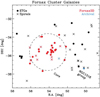 |
Fig. 1 Location on the sky of the ETGs (circles) and LTGs (crosses) with mB < 15 mag in the Fornax cluster. The dashed circle marks the virial radius of the cluster and corresponds to about 0.7 Mpc, as determined by Drinkwater et al. (2001). The red symbols show F3D galaxies while the blue symbols correspond to NGC 1316 (filled circle) and NGC 1365 (cross) for which MUSE data are already available in the ESO Science Archive Facility. |
Main properties of the F3D galaxies.
MUSE pointings of the F3D galaxies.
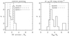 |
Fig. 2 Left panel: spatial coverage of the MUSE central pointings of the F3D ETGs in units of 30 arcsec ∕Re (histogram) compared to the ATLAS3D (Cappellari et al. 2011; dotted line) and MaNGA (Bundy et al. 2015; primary sample: dashed line, secondary sample: dash-dotted line) surveys. Right panel: spatial coverage of the MUSE halo pointings of the F3D ETGs down to μB = 25 mag arcsec−2 in units of R25∕Re (histogram) compared to the MASSIVE (Greene et al. 2015, dotted line) and SLUGGS (Foster et al. 2016, dashed line) surveys. |
3 Observations and data reduction
The integral-field spectroscopic observations of the F3D sample galaxies were carried out with MUSE mounted on the Yepun Unit Telescope 4 at the ESO Very Large Telescope in Chile. MUSE was configured in Wide Field Mode (Bacon et al. 2010) that ensured a 1 × 1 arcmin2 field coverage with 0.2 × 0.2 arcsec2 spatial sampling and a wavelength range of 4650–9300 Å with nominal spectral resolution of 2.5 Å (FWHM) at 7000 Å and spectral sampling of 1.25 Å pixel−1.
Data were taken in service mode between July 2016 and December 2017 (Table 2). Typical integration times of on-source exposures were 12 min for the central pointings and 10 min for the middle and halo pointings. The on-source exposures were dithered by a few arcseconds and rotated by 90° in order to average the spatial signature of the 24 integral-field units on the field of view. For the majority of the targets, dedicated sky exposures of 3 min were scheduled within each observing block, immediately before or after of each on-source exposure.
The data reduction was performed with the MUSE pipeline version 1.6.2 (Weilbacher et al. 2012, 2016) under the ESOREFLEX environment(Freudling et al. 2013). The reduction cascade included bias and overscan subtraction, flat fielding to correct the pixel-to-pixel response variation, wavelength calibration, determination of the line spread function, illumination correction with twilight flats to account for large-scale variation of the illumination of the detectors, and illumination correction with lamp flats to correct for the edge effects between the integral-field units. For each galaxy, the twilight exposures were combined following the same observing pattern of the target observations, producing a master twilight datacube that was used to determine the effective spectral resolution and its variation across the field of view.
The sky subtraction was done by fitting and subtracting a sky model spectrum on each spaxel of the field of view. The sky model was either evaluated on dedicated sky observations or on the edges of the exposure for the smallesttargets, where the contribution of the galaxy was negligible. The flux calibration and the first-order correction of the atmospheric telluric features were obtained using the spectro-photometric standard star observed at twilight.
A fully reduced “pixel table” was produced from each exposure. For each galaxy, the pixel tables were aligned using reference sources and then combined in an single datacube. For each individual galaxy, a datacube with the sky residuals was also produced. It was obtained by combining the sky-subtracted pixel tables of the offset sky exposures in a single datacube following the same rotation pattern as the target observations.
An additional cleaning of the residual sky contamination was achieved with the Zurich Atmospheric Purge algorithm (ZAP; Soto et al. 2016), which exploits principal component analysis to characterise and subtract the sky residuals from the observations. The principal components of the sky residuals were evaluated on the sky-residual datacubes or at the edges of the sky-subtracted target datacube, depending on the spatial extension of the galaxy. The algorithm was run within the ESOREFLEX environment, using the dedicated workflow distributed with the MUSE pipeline. For a number of targets, the results were compared by running ZAP on the individual exposures before the creation of the final datacube, and on the final datacube itself. No significant differences were found. Therefore, the adopted strategy was to clean the final combined datacube and not the individual exposures.
4 Data analysis
The data analysis was built on tools and techniques that were developed for the SAURON, ATLAS3D, and CALIFA surveys. The Voronoi binning scheme by Cappellari & Copin (2003) was used to spatially bin the data to a minimum S/N per pixel to ensure a reliable extraction of the relevant parameters of the stellar and ionised-gas kinematics and stellar populations. The stellar kinematics was computed using the Penalised Pixel-Fitting code (pPXF; Cappellari & Emsellem 2004; Cappellari 2017). Emission-line morphologies and kinematics were derived using the Gas and Absorption Line Fitting code (GandALF; Sarzi et al. 2006; Falcón-Barroso et al. 2006). The line-strength indices for the stellar population analysis were extracted as well. In the remainder of this section, the specific details about how all these methods were applied to the F3D data are provided.
The Voronoi binning process started by selecting spaxels with a minimum S/N of three (median value per pixel) as estimated using the pipeline variance cube. This was necessary to avoid poor quality spaxels which could introduce undesired systematic effects in the data at low surface-brightness regimes, that are not straightforward to account for (e.g. affecting the accuracy of the sky subtraction). In order to produce maps that match the surface photometry of the galaxies, all spaxels within the isophote level where ⟨S∕N⟩~ 3 were selected. Given that the survey has a wide range of scientific goals with different requirements, Voronoi binned maps were produced to S∕N = 40 and 100.
The combination of individual dithered observations introduced spatial correlations between neighbouring spatial and spectral pixels in thefinal combined data. This mainly affected the variance spectra resulting from the propagation of uncertainties at every step of the full data reduction process. While in principle, this effect could be accounted for by computing the covariance matrix for this combination step, the sheer volume of the data made this approach unfeasible and computationally very expensive. Instead, a more pragmatic solution was adoped: that followed by the CALIFA survey (García-Benito et al. 2015), empirically characterising the level of correlation and correcting for it during the Voronoi binning process. However, as discussed in Sect. 5, the level of covariance in the data is relatively small compared to that in the CALIFA survey.
The extraction of the stellar kinematics in the Voronoi binned spectra is restricted to the 4750–5500 Å wavelength range. Use of the full wavelength coverage of the MUSE datacube did not alter the results in any significant manner. The advantages were a major speed up in computation time and avoiding to correct the stellar templates for spectral resolution changes along wavelength. In such a short spectral range, only a low-order additive polynomial (degree = 8) was necessary to compensate for differences in calibration between the F3D data and templates. The MIUSCAT models (Vazdekis et al. 2012) were adopted as stellar templates for the extraction of the stellar kinematics. A subset of 65models was selected that uniformly sample age (from 0.1 to 15.8 Gyr) and metallicity (from − 2.32 to 0.22 dex). This subset was a good representation of the entire MIUSCAT library and very few differences were found between the two sets.
By contrast with the stellar kinematics, for which the applied spatial binning was based on the S/N estimated from the stellar continuum, the analysis of the emission-line properties was done on a spaxel-by-spaxel level, in order to capture the structure in the emission-line distribution at the highest spatial resolution provided by the data. GandALF was used in the wavelength range between 4800–6800 Å, using only a two-component reddening correction to adjust for the stellar continuum shape and for the observed Balmer decrement. Similar to the standard setup used in Sloan Digital Sky Survey data in the value-added catalogue ofOh et al. (2011), a table was created with fitted emission-line species and relative dependencies. The stellar kinematics assumed for each spaxel is that of the Voronoi bin each spaxel belongs to. Given the large differences in wavelength of the different emission lines, spectral resolution variations are accounted for during the fitting process. Spatial variations of the spectral resolution within the field of view of MUSE were not taken into account.
The study of the stellar population requires high S/N. It is for that reason that the line-strength analysis was based on the Voronoi binned data. Since emission-line contamination of stellar absorption features is an issue, the procedures summarised above were repeated with GandALF for the Voronoi binned spectra. Nebular emission as a whole was conservatively considered as detected when the amplitude-over-noise ratio was above three for all major lines (e.g. Hα, Hβ, [N II], and [O III]). Emission was removed from the spectra when, based on the GandALF uncertainties there was a 68% probability that the no-emission hypothesis could be rejected. Line-strength indices were computed in the LIS system (Vazdekis et al. 2010). This approach minimised some of the major intrinsic uncertainties associated with the popular Lick/IDS system (González 1993). This line-strength index system is based on flux-calibrated spectra with a constant resolution as a function of wavelength providing three different resolutions, namely 5, 8.4, and 14 Å (FWHM). The resolution of 8.4 Å, which is appropriate for studying low- to intermediate-mass galaxies, was usually sufficient for F3D scientific aims.
In addition to line-strength indices, the use of regularised solutions in pPXF was also explored to derive star formation histories across the entire MUSE maps. This has the potential to reveal the formation sequence of the different components in galaxies and therefore provide a much more complete evolutionary picture. The first results following this approach are presented in Pinna et al. (2018) to study the origin of the thick disc component in FCC 170.
The instrumental spectral resolution can be determined by the MUSE pipeline by recovering the full shape of the line spread function using a series of dedicated arc lamp observations. The instrumental spectral resolution varies with wavelength, integral-field unit, and slice. The galaxy observations were composed of exposures taken at varying orthogonal position angles, thus the combined spectra are influenced by each of these effects. The following strategy was adopted to measure the resulting line spread function. For each galaxy, N twilight datacubes were combined using the same observational pattern (including rotations and offsets) as the N galaxy exposures. The resulting effective instrumental broadening function was derived from the combined twilight cubes by applying pPXF with a solar-spectrum template. The process was divided in a number of wavelength intervals and for each spaxel in order to measure the variation of the fitting parameters with wavelength and position over the field of view. On average, the instrumental spectral resolution was FWHMinst ~ 2.8 Å with little variation (<0.2 Å) with wavelength and position over the field of view. This showed that the effect of having combined exposures taken at different rotations (i.e. of having combined the signal from different integral-field units) is an increase of the mean instrumental FWHM and a homogenisation over the field of view and wavelength. A modest spatial dependence of the FWHM remains, however. The twilight maps can be used to correct for this where needed (e.g. when the velocity dispersion is close to or less than the instrumental resolution).
5 Data quality
This section describes the analysis of the MUSE data obtained for FCC 167 to assess the quality of the data, with attention to i) the S/N per spaxel down to surface brightness of μB = 25 mag arcsec−2, which includes a quality check of the subtraction of the sky emission; ii) the correction for the atmospheric telluric absorption which is key to constraining the low-mass end of the IMF from a spectral analysis; iii) the quality of the relative flux calibration, which is related to the ability to measure IMF-sensitive absorption-line index (e.g. aTiO, TiO1, and TiO2); iv) the quality of the absolute flux calibration, which is important for the extraction of reliable emission-line flux values and thus derive, for instance the star-formation rate or luminosity of PNe.
The S0/a galaxy FCC 167 is on the northeast side of the Fornax cluster, located at about 0.6° (corresponding to 222 kpc) from NGC 1399 and at a distance of 21.2 Mpc from surface-brightness fluctuations (Blakeslee et al. 2009) (see Table 1). The three pointings for this object cover the central and middle regions and the outskirts (Table 2). Figure 3 shows the MUSE pointings on an r-band image obtained with the Fornax Deep Survey (Iodice et al. 2016; Venhola et al. 2017) and Fig. 4 comparesthe MUSE reconstructed image for the combined mosaic with the isophotes in the r-band derived from the deep VST image shown in Fig. 3. The top panel of Fig. 4 demonstrates that the individual pointings were correctly aligned before combining them, whereas the lower panel shows more quantitatively by means ofa major-axis cut how well the surface-brightness radial profile of the MUSE reconstructed image, after arbitrarily rescaling, follows that of the VST image. This comparison also illustrates that the overall level of the sky subtraction has been determined correctly, in particular down to the target surface-brightness level of μB = 25 mag arcsec−2 and out to R25∕Re ~ 3.5.
The HST images obtained by Jordán et al. (2007) with the Advanced Camera for Survey (ACS) in the F850LP passband, which covers the red end of the MUSE spectra (above 8000 Å), allow a further check of the absolute flux calibration. Including a small systematic correction to account for the fact that this passband extends slightly beyond the MUSE data, the average flux density of the spectra within the F850LP passband is within 10% of the flux density measured by the HST images.
The quality of the spectroscopic data is best revealed through the comparison with a physically-motivated fit to both the stellar continuum and nebular emission. Figure 5 shows the best GandALF fit to the two aperture spectra extracted at the locations indicated in Fig. 4: one centred on the nucleus of FCC 167 and the other at about 80 arcsec to the north, where the surface brightness of the galaxy is comparable to the sky background. Only dust reddening was included to correct the continuum shape, as opposed to resorting to a high-order multiplicative polynomial correction which may adjust for possible shortcomings in the data (such as an imperfect relative flux calibration). For both aperture spectra, Fig. 5 shows that the quality of the data is excellent, leading to residuals with little or no significant structure, except for a) systematic fluctuations introduced by template mismatch in the case of the GandALF fit to the very high S/N nuclear spectrum and b) some sky-subtraction residuals in the case of the outer spectrum, due to bands of weak sky emission-lines (between 5900 and 6650 Å). The residuals do not show the presence of low-frequency fluctuations, thus indicating that the relative flux calibration is under control.
To further evaluate the spectral quality, the signal-to-fit-residual-noise ratio (S/rN), was computed in the Voronoi-binned spectra and based on the results of the adopted standard pPXF fitting procedure. This S/rN is a more conservative measurement of the quality of the MUSE spectra than the formal S/N values based on the variance spectra returned by the data reduction and their formal propagation during the spatial binning process. This is because the fit residuals can also capture systematic errors in the data reduction and in particular spatial covariance introduced during the combination of individual dithered observations.
Figure 6 (top panel) shows the values of the S/rN ratio as a function of the mean r-band surface brightness inside the Voronoi bins obtained imposing a formal S∕N = 40 before further accounting for spatial correlations, as described in García-Benito et al. (2015). This illustrates the negative impact of spatial correlations, as the target S∕N = 40 is not met at first in the outskirts of FCC 167 where the data were combined in larger bins. However, the depth of the exposure was sufficient to reach the target S∕N = 25 per spaxel and resolution element around 5500 Å within the adopted fitting range at a surface brightness of μB = 25 mag arcsec−2 (corresponding μr ~ 25 mag arcsec−2 for old stellar populations).
To better quantify the impact of spatial correlations, Fig. 6 (lower panel) shows the value of correlation ratio β =rN∕N = (S∕N)∕(S∕rN) per Voronoi bin as a function of the number of spaxels Nspaxels between the noise level in the fit residuals rN and formally propagated noise N. As found in García-Benito et al. (2015), β is a linear function of log(Nspaxels) for relatively small bin sizes, although the spatial correlation in the MUSE cubes is much smaller than those in the CALIFA data. For larger bins in low-surface brightness and progressively more sky-dominated regions, β(N) increases faster as a function of bin size, so that the overall quadratic form 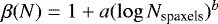 provides a better way to characterise the spatial correlations. Using this parametrisation to account for covariances during the Voronoi binning brings the quality of the outer binned spectra for FCC 167 back to the S∕N = 40 target (see Fig. 7 for the resulting kinematics).
The use of the MOLECFIT (Smette et al. 2015) and SKYCORR (Noll et al. 2014) procedures provides a better correction for atmospheric telluric absorption than the adopted one based on the use of telluric standards (Sect. 4). Most of the improvement is in the quality of the sky-subtraction, and this will be applied on an individual spectrum basis depending on the science goals.
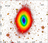 |
Fig. 3 r-Band image of FCC 167 from the Fornax Deep Survey with VST (Iodice et al. 2016; Venhola et al. 2017). The 1 × 1 arcmin2 MUSE pointings are shown in black. The black dashed ellipse corresponds to the isophote at μB = 25 mag arcsec−2, while the right ascension and declination (J2000.0) are given in degrees on the horizontal and vertical axes of the field of view, respectively. |
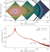 |
Fig. 4 Top panel: MUSE reconstructed image of the combined mosaic of FCC 167 compared with isophotes of the r-band VST image shown in Fig. 3. The black isophotes cover the range between μr = 16.6 and 22.6 mag arcsec−2 and are spaced by 1 mag arcsec−2. The grey isophote corresponds to μB = 25 mag arcsec−2. The blue and orange circles indicate, respectively, the position of the central and outer apertures selected for testing the spectral quality of the F3D data (see Fig. 5). The red dashed lines mark the 2 arcsec wide aperture along the galaxy major axis (P.A. = 3.9°) where the surface-brightness radial profile plotted in the bottom panel was extracted. Bottom panel: surface-brightness radial profile along the major axis of FCC 167 from the MUSE reconstructed image (red points) and r-band VST image (black points). The sky level of MUSE (horizontal continuous line) and μB = 25 mag arcsec−2 (horizontal dashed line) are shown for comparison. |
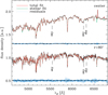 |
Fig. 5 GandALF fits to the central (top panel) and outer aperture (bottom panel) spectra extracted from the MUSE data of FCC 167 (see Fig. 4). To allow a more direct comparison between these two spectra (black lines) and their respective GandALF fits (green and red lines), both data and models were normalised and rescaled. The residuals obtained by subtracting the model from the spectrum are also shown (bluepoints). These models used the entire MILES (Blasquez et al. 2006) stellar library as stellar templates to achieve the best possible fit. At the same time, to ensure a physically-motivated model only reddening by dust was used to adjust the templates to the observed shape of the stellar continuum. The position of the most prominent [O I] sky emission lines is indicated. |
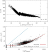 |
Fig. 6 Top panel: quality of the Voronoi-binned spectra for a target S∕N = 40 as a functionof r-band surface brightness in MUSE data of FCC 167. The S/rN ratio between the median value of the flux and the noise level in the fit residuals is used as a more conservative measure of the spectral quality. Lower panel: level of spatial correlation in the MUSE data of FCC 167. The covariance ratio β = rN∕N between the fit residual noise and the formally propagated noise increases as function of bin size (or number ofspaxels) in each Voronoi bin, although much less than in the CALIFA data (blue line). The β trend is well described by a quadratic form in logNspaxels (red line). |
6 Illustrative initial results
This sectionpresents some preliminary results obtained for the main science topics listed in Sect. 1. A detailed analysis anddiscussion will be presented in forthcoming papers.
6.1 Embedded discs in fast rotating ETGs
Figure 7 shows the stellar kinematic maps of the mean velocity v, velocity dispersion σ and the higher-order moments h3 and h4 of the line-of-sight velocity distribution for FCC 167, derived from the S∕N = 40 Voronoi-binned MUSE data. The presence of a large-scale kinematically cold disc component is beautifully brought out by the h3 and h4 maps. The median errors in the maps are 5 and 6 km s−1 for v and σ, respectively and 0.025 for both h3 and h4. To further reduce these errors for the purpose of constructing dynamical models, the data were binned to a S∕N = 100 target (see Fig. 8). This brings down the previous errors on v and σ to 2.5 and 3.5 km s−1 and to 0.012 for h3 and h4. The formal uncertainties on the stellar kinematic parameters returned by pPXF were rescaled assuming that the χ2 of the best-fitting model matches the number of degrees of freedom. The rescaled uncertainties capture the systematic deviations due to template mismatch and spatial correlations in the Voronoi bins in the centre and outskirts of the sample galaxies, respectively.
The stellar kinematic maps obtained for FCC 167 with the S∕N = 100 Voronoi-binned MUSE data were used as constraints for Schwarzschild orbit-based dynamical models in order to derive the internal orbital structure using the approach described in van den Bosch et al. (2008) and Zhu et al. (2018). The observed surface-brightness distribution of FCC 167 was fitted with a bi-axial multi-Gaussian-expansion model (Emsellem et al. 1994; Cappellari 2002), and deprojected to a three-dimensional triaxial model for the stellar luminosity by adopting a set of viewing angles (ϑ, ψ, ϕ). Multiplication by a constant stellar M/L provides the intrinsic mass density distribution of the stars. The three viewing angles relate directly to the axis ratios p = b∕a and q = c∕a and the scale factor u = aobs∕a, where a ≥ b ≥ c are the semi-axes of the constituent triaxial Gaussian density distributions and aobs is the observed major axis scale-length.Varying p and q allows exploring different intrinsic triaxial shapes. A spherical dark matter halo was added with a Navarro–Frenk–White (NFW) profile (Navarro et al. 1997) and concentration parameter c fixed according to its relation with the virial mass M200 from cosmological simulations (Dutton & Macciò 2014). The resulting total mass distribution provides the gravitational potential. Thus, the dynamical models have five free parameters: the stellar M/L; the axis ratios p and q and scale factor u of the triaxial stellar density distribution and the dark halo mass M200. The gravitational potential is static and figure rotation is not included in the model.
For each choice of parameters, a large number of stellar orbits was computed to be able to match the data. The number of orbits sampled in the space of the three integrals of motion (E, I2, I3) was (65, 15, 15), with an additional overall factor 33 resulting from dithering to create an orbit bundle (see van den Bosch et al. 2008), leading to a total of 39 4875 orbits per model. This large number of orbits is needed to do justice to the high quality of the data. The orbital weights were determined by simultaneously fitting the orbit-superposition models to the projected and de-projected luminosity density and the two-dimensional line-of-sight stellar kinematics, in other words, the maps of v, σ, h3, and h4. As shown in Fig. 8, the model with the best-fitting global parameters stellar M∕L = 5.5 M⊙∕L⊙, q = 0.60, p = 0.965, u = 0.966 (which corresponds to an inclination angle of 77.6°), and M200 = 6.4 × 10¹² M⊙ matches the stellar kinematic maps well from the inner to the outer regions.
The internal dynamical structure of each model is described by the distribution of orbital weights in integral-of-motion space. One way to visualise it is to plot the variation of λz with radius r, where λz is the circularity of orbit defined as the angular momentum around the short axis z normalised by that of the circular orbit at the same binding energy, and r is the time-averaged radius of each orbit. The result for the best-fitting model of FCC 167 is shown in the left panel of Fig. 9. Most orbits have λz < 0.25, comprising the bulge in the inner region, and contributing to the halo in the outer region. The diagram also reveals two embedded disc components: a warm (0.25 < λz < 0.8) component and a cold (0.8 < λz < 1.0) component. The cold component resembles a thin disc similar to those seen in spiral galaxies. The warm orbits constitute a thick disc with weaker rotation. The surface brightness profiles of the hot, warm, and cold orbital components are shown in the right panel of Fig. 9 and the two-dimensional surface brightness distributions of these three components are shown in the left panels of Fig. 10. The right panels of Fig. 10 show the result of a standard two-dimensional photometric decomposition into a bulge and disc, performed by using the GALFIT package (Peng et al. 2010) on the MUSE reconstructed image of FCC 167 (see Fig. 8). The surface brightness of the cold component matches the photometric disc, with comparable scale length (~ 30 arcsec or ~3 kpc). The photometric bulge appears more boxy than the hot dynamical bulge, but both components have comparable effective radius (~ 18 arcsec or ~2 kpc). The light distribution of the combined warm and hot component (see lower-right panel of Fig. 10) matches quite well the isophotes of the photometric bulge. This demonstrates that dynamical decomposition is needed to disentangle the warm and hot components.
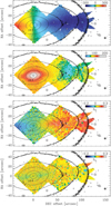 |
Fig. 7 Stellar kinematic maps of the mean velocity v, velocity dispersion σ, and higher-order moments h3 and h4 of the line-of-sight velocity distribution for FCC 167 derived from the S∕N = 40 Voronoi-binned MUSE data with the r-band isophotes (black lines) shown in Fig. 4. |
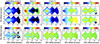 |
Fig. 8 Best-fitting Schwarzschild orbit-based dynamical model of FCC 167. Top and middle panels: observed and best-fitting model of the surface brightness SB, mean velocity v, velocity dispersion σ, and higher-order moments h3 and h4 of the line-of-sight velocity distribution, respectively. Bottom panels: residuals obtained by subtracting the best-fitting model from data. |
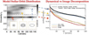 |
Fig. 9 Orbital and photometric decomposition of FCC 167. Left panel: orbit distribution in the phase space of circularity λZ vs. intrinsic radius r, as derived from the best-fitting orbit-superposition model shown in Fig. 8. Grey-scale colours indicate the orbital density in phase space. The horizontal dashed lines separate stars in highly-circular cold thin-disc orbits (λZ > 0.7) from those following dynamically warm thick-disc motions (0.2 < λZ < 0.7) and those in the non-rotating bulge and stellar halo (λZ ~ 0). Right panel:stellar surface-density profiles of FCC 167. The grey lines trace the profiles of a classical exponential disc and Sérsic bulge as derived from a standard bulge-disc decomposition, whereas the blue, orange, and red lines follow the projected surface brightness of the dynamically cold, warm (thick disc), and hot (bulge) components, respectively. |
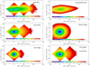 |
Fig. 10 Two-dimensional light distribution for the dynamical and photometric components of FCC 167. Left panel: two-dimensional distribution of light from each of the dynamical components, as derived from the best-fitting orbit-superposition model shown in Fig. 8: dynamically cold, warm (thick disc), and hot (bulge) componentsare shown in the top, middle and lower panel, respectively. Right panel: two-dimensional distribution of light from each of the photometric components, Sérsic bulge (middle panel) and exponential disc (top panel), as derived from the fit of the light distribution of the MUSE reconstructed image shown in Fig. 4. In the lower panel is shown the resulting image from the superposition of the hot (bulge) and warm (thick disc) dynamical components. In all panels, the colour bar indicates the surface brightness levels adopting an arbitrary zero point. |
6.2 Photometric and kinematic disc signatures in ETGs
The radial profiles of the mean velocity and velocity dispersion of FCC 167 were derived within a 2 arcsec wide aperture at P.A. = 3.9° crossing the nucleus (Fig. 11) from the kinematic maps obtained after Voronoi binning to a S∕N = 40. MUSE data map the stellar kinematics out to the unprecedented galactocentric distance of 115 arcsec (about 11.8 kpc) with very low uncertainties (≤10 km s−1) and definitely confirm the presence of several localised substructures, which were previously identified by Bedregal et al. (2006).
The mean velocity reaches a maximum of v ~ 220 km s−1 at R ~ 70 arcsec and it remains almost constant outto R ~ 100 arcsec. The velocity dispersion decreases from a central maximum value of σ ~230 km s−1 to σ~ 90 km s−1 at R ~ 70 arcsec. At larger radii, the velocity dispersion increases again to σ ~ 110 km s−1 for 70 ≤ R ≤ 115 arcsec. Sucha local minimum is already visible in long-slit data by Bedregal et al. (2006), although they did not comment on it. The σ-drop seems to be more pronounced in the long-slit data (σ ~ 85 km s−1 at R ~ 70 arcsec), but it is consistent within the errors with the MUSE measurements.
For 70 ≤ R ≤ 115 arcsec, light is still mapping the bright regions of the disc in the range of surface brightness 21 ≤ μr ≤ 24 mag arcsec−2 (Fig. 4). The σ-drop corresponds to a plateau in the surface-brightness radial profile at R ~ 70 arcsec. At the same radius, the isophotes show an increasing flattening (ϵ ~ 0.6) and a twisting of 10 degrees (Caon et al. 1994).
A Gaussian filter of the r-band VST image of FCC 167 given in Fig. 3 was performed by using the IRAF1 task FMEDIAN. The ratio between the original and filtered image gave the high-frequency residual image shown in Fig. 12. In the inner ~60 arcsec, it reveals a boxy structure which ends with a spiral-like arm and a bright knot at R ~ 70 arcsec on both sides along the major axis of the disc. This is the distance where the σ-drop in kinematics and break in the surface-brightness radial profile are observed. Thus, it seems reasonable to conclude that this feature is more likely a substructure in the disc, which produces a broadening of the line-of-sight velocity distribution.
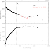 |
Fig. 11 Stellar kinematics of FCC 167 extracted from the MUSE data (black points) at P.A. = 3.9° within the2 arcsec wide aperture crossing the nucleus shown in Fig. 4. The mean velocity v (bottom panel) and velocity dispersion σ (top panel) are given. The mean errors of the data are shown in the lower-right corner of each panel. The velocity dispersion is compared to the long-slit spectroscopic data obtained by Bedregal et al. (2006) for the north side of the galaxy (red points). The vertical dashed line corresponds to the effective radius. |
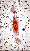 |
Fig. 12 High-frequency residual image obtained from the r-band VST image of FCC 167. The 1 × 1 arcmin2 MUSE pointings are overplotted in black. The black dashed lines mark the 2 arcsec wide aperture at P.A. = 3.9°, where the stellar kinematics shown in Fig. 11 was extracted from the MUSE data. The right ascension and declination (J2000.0) are given in degrees on the vertical and horizontal axes of the field of view, respectively. |
6.3 Stellar population in the outskirts of ETGs
One of the ambitious goals of the F3D project is to study the stellar age, metallicity, and α-element abundance in the outskirts of ETGs, out to the faint regions of their stellar halos. This will provide insight into the assembly history of galaxies.
Figure 13 presents the map of the Mg b index, which shows a clear negative outwards gradient towards lower metallicity, and reveals the presence of low-metallicity objects along the line-of-sight of FCC 167 at about 40 arcsec slightly northwest to the nucleus. The line-strength indices of Hβ, Mg b, Fe5270, Fe5335, and Fe5406 were measured in the two selected apertures in the middle (μr ~ 21.3 mag arcsec−2) and halo pointing (μr ~ 23 mag arcsec−2) shown in Fig. 13. They were fitted with a single-stellar-population Markov-chain-Monte-Carlo code, using the MILES models (Vazdekis et al. 2010) to provide the stellar age, metallicity, and α-element abundance ratio. The results are shown in Fig. 14 and suggest that in the outskirts of FCC 167 the mean stellar population has an α-element abundance [Mg/Fe] ~ 0.8−0.16 dex and an average age in the range 2.5–5 Gyr. These initial results are based on the standard data reduction, and demonstrate that the stellar population properties can be traced well into its outskirts.
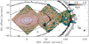 |
Fig. 13 Mg b map of FCC 167 with the r-band isophotes (black lines) and B-band isophote (grey line) shown in Fig. 4. The orange and red circles indicate the location of two selected apertures where the Hβ, Mg b, Fe5270, Fe5335, and Fe5406 line-strength indices were measured and fitted in order to constrain the stellar population properties, as shown in Fig. 14. |
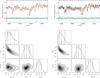 |
Fig. 14 Stellar population properties from the two selected apertures in the middle (left panels) and halo pointing (right panels) of FCC 167 shown in Fig. 13. Top panels: rest-frame spectra (black lines), best-fitting models (red lines), and residuals obtained by subtracting models from spectra (green points). Bottom panels: posterior distributions for the age, metallicity [M/H], and α-element abundance [Mg/Fe]. The dashed lines overplotted on the histograms indicate the 16%, 50%, and 84% percentiles of the marginalised distributions. |
6.4 Globular clusters and planetary nebulae
The MUSE observations also give access to GCs and PNe as discrete tracers of the underlying gravitational potential of the galaxies. First representative results on the detection of GCs and PNe in FCC 167 are presented below.
GCs detection in FCC 167 – the IMFIT algorithm (Erwin 2015) was used to model the surface-brightness distribution of FCC 167 extracted from a broad combined wavelength range of the MUSE datacubes. The resulting image was subtracted to highlight underlying structures and point sources. The locations of GCs were determined with DAOStarFinder, a Python implementation of the DAOPHOT algorithm (Stetson 1987) and were cross-referenced with the positions of GC candidates from the HST/ACS GC catalogue (Jordán et al. 2015). For FCC 167, the ACS study did not extend into the outer halo pointing, so additional GC candidates were identified directly from the MUSE data. The redshifts of these additional GC candidates were checked to confirm that these are really GCs in the FCC 167 halo rather than stars or background galaxies.
The seeing of the observations for FCC 167 was about 0.9 arcsec (FWHM) corresponding to σ =0.38 arcsec (about two pixels). Therefore, the spectra were extracted within a circular aperture with a radius of two pixels. The contamination from the galaxy light was removed by subtracting the galaxy spectrum in an annulus around the GC. The radial velocities of the GCs were determined via full spectral fitting with pPXF. Figure 15 shows the map of the mean stellar velocity of FCC 167 after Voronoi binning to a S∕N = 100 with extracted GCs colour-coded by their radial velocities. While the stellar population properties can be determined only for GCs with high S/N, the low S/N of the majority of detected GCs still allows for radial velocity estimates.
PNe in FCC 167 – to illustrate the potential of the MUSE observations to detect and study the PNe in the central regions of galaxies out to the distance of the Fornax cluster, Fig. 16 shows a map of the flux of the [O III]λ5007 emission from the central pointing of FCC 167 obtained when seeing conditions were optimal. In addition to a central disc of diffuse ionised gas (Viane et al. 2018, in prep.), the presence of a large number of point sources is immediately evident. The most prominent ones are highlighted in Fig. 16 and are confirmed as PNe. Figure 16 also shows how it becomes progressively more difficult to establish the presence of PNe towards the central regions. This is due to an increasing background of [O III]λ5007 emission that consists, in fact, mostly of correlated false detections. As the amplitude of false detections scales with the Poisson noise level in the stellar continuum of the MUSE spectra, this increase in the spurious emission towards the centre of the galaxy makes it more difficult to identify fainter PNe.
A preliminary analysis of the PNe population in FCC 167 indicates that PNe can be detected down to the absolute [O III]λ5007 magnitude M5007 = −2.7, or nearly two magnitudes below the bright cutoff of the PNe luminosity function (Ciardullo et al. 1989), while being complete at M5007 = −3.7. A detailed investigation of the PNe population of this and other F3D galaxies is under way. Furthermore, the unique depth of the MUSE stellar-population measurements will allow to check the connection between the PNe properties and those of their parent stellar populations (e.g. Buzzoni et al. 2006) both a) in a spatially consistent fashion and b) far out into the outskirts of F3D galaxies. In these outer regions narrow-band or slitless spectroscopic measurements from the literature (see e.g. Spiniello et al. 2018, for specific Fornax measurements) will complement well the measurements from the F3D data.
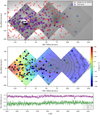 |
Fig. 15 Illustration of GC extraction from MUSE data of FCC 167. Top panel: residual image obtained by subtractingthe IMFIT surface-brightness model of FCC 167 from the galaxy surface-brightness distribution extracted from MUSE data. The GC candidates from MUSE data (blue circles) and GCs in the HST/ACS GC catalogue (Jordán et al. 2015; red crosses) are shown. Middle panel: map of the mean stellar velocity of FCC 167 shown in Fig. 8 and radial velocities of the GCs. Bottom panel: spectra of two MUSE GCs with S∕N ≈ 25 (purple line) and 5 (green line) whose location is indicated in the top panel by the filled purple and open green triangles, respectively. |
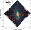 |
Fig. 16 Map of the flux of the [O III]λ5007 emission from the central pointing of FCC 167. The extended disc is clearly visible. The detected planetary nebulae are indicated by red circles. [O III]λ5007 flux values are shown on a logarithmic scale and in 10−20 erg cm−2 s−1. |
6.5 Late-type galaxies
Figure 18 shows initial results of the emission line analysis performed with pPXF and GandALF on the late-type galaxy FCC 312. This is an Scd galaxy on the east side of the cluster, at about two degrees from NGC 1399. It is the most extended disc galaxy in the F3D sample, with a major axis diameter of 4.7 arcmin, with a prominent flare on both sides of the outer disc regions. The three MUSE pointings map the light from the centre out to the flaring regions of the disc, which are more pronounced on the southeast side (Fig. A.1). Here, initial results are reported forthe central pointing. The ten LTGs in the sample, which span the full range in the Hubble sequence of barred and unbarred spirals, from Sa to Sd and Sm types, will be presented and discussed in a forthcoming paper.
The top row of Fig. 18 shows the maps of the total flux from the [N II]λ6583 emission and of the corresponding velocity and velocity dispersion. The flux map is characterised by the conspicuous presence of regions withgas ionised by hot stars, and, interestingly, a loop-like feature in the southeast side suggestive of expanding gaseous bubbles produced by stellar feedback. While the velocity dispersion map does not show an excess in the loop, which could originate from shocks with the cold phase of the interstellar medium produced by the outwards motion, the velocity field shows an offset in the region as compared to the rest of the galaxy. The [N II]λ6583/Hα and [O III]λ5007/Hβ line ratio maps displayed in Fig. 18 also present conspicuous extra-planar ionised regions in the area of the loop-like feature, as well as significant variation in the [O III]λ5007/Hβ line ratio amongst the different H II regions. It is possible that this feature is another example of an extra-planar echo of activity in the galactic nucleus (see Keel et al. 2012). The spaxel-by-spaxel BPT diagram (Baldwin et al. 1981) of Fig. 18 shows that several line-excitation mechanisms are present, including that from AGN activity.
The Hα de-reddened flux map is shown in thebottom row of Fig. 18, together with maps of dust extinction, as measured in the nebular lines and from the stellar continuum with the usual uniform dust screen approximation across the galaxy. The latter modifies the entire spectrum, and is thus in addition to the extinction affecting nebular lines only. The nebular extinction map is derived using the standard Balmer decrement approach, and accounting for the uniform dust screen contribution. This differentiated approach to measure the extinction allows deriving more accurately the effects of dust mixed with gas in star forming regions. Comparing the extinction maps in Fig. 18 one sees that the continuum-derived dust component in the galaxy is more uniformly distributed and concentrated in the disc plane, as expected.
Interestingly, the regions with elevated Hα flux (and thus star formation rate) are more heavily dust-obscured. To illustrate this, Fig. 19 shows the correlation found between the dust extinction affecting nebular lines and Hα luminosity in the same region. The origin of this correlation can be understood if regions of elevated star formation are also the regions of more substantial gas content, which is to be expected from the Kennicutt–Schmidt star-formation relation (Schmidt 1959; Kennicutt 1998). More ionising photons coming from hot stars combined with more hydrogen atoms would lead to more luminous Hα emission. Furthermore, more gas can, in principle, be translated into more dust content as well, but this correlation can depend on the metal content of the gas, since metal-poor regions are inefficient in producing dust grains. This can partly explain the scatter in the correlation. Another factor that can add scatter is the geometry of the dust distribution in the individual star-forming systems, which will determine the fraction of escaping photons. A study of this correlation for all F3D LTGs will be presented in a future paper.
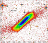 |
Fig. 17 Digitized Sky Survey image of FCC 312. The 1 × 1 arcmin2 MUSE pointings are shown in black. The black dashed ellipse corresponds to the isophote at μB = 25 mag arcsec−2, while the right ascension and declination (J2000.0) are given in degrees on the horizontal and vertical axes of the field of view, respectively. |
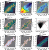 |
Fig. 18 Emission-line analysis for the central regions of FCC 312. Top panels: maps of the total flux, mean velocity and velocity dispersion along the line-of-sight from the [N II]λ6583 nebular emission. Middle panels: maps of the [N II]λ6583/Hα and [O III]λ5007/Hβ line ratios and corresponding BPT diagram. Bottom panels: maps of the de-reddened Hα flux, extinction on the nebular lines, and extinction derived from the stellar continuum. Velocities and velocity dispersions are in km s−1, reddening values are in magnitude, line ratios and fluxes are shown in a logarithmic scales, with the latter in units of 10−20 erg cm−2 s−1. Grey areas in the maps refer to regions where the S/N of the relevant lines was not sufficiently elevated to firmly exclude a false positive detection. These levels were established in regions devoid of emission well above and below the equatorial plane of the galaxy. |
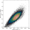 |
Fig. 19 Correlation between the dust extinction affecting nebular lines and Hα luminosity in the same region, corrected for total extinction. Regions with elevated star formation rate are also heavily dust obscured. |
7 Concluding remarks
This paper demonstrates that MUSE enables a comprehensive study of the internal orbital structure and stellar populations of a sample of galaxies inside the virial radius of the Fornax cluster. The design of the survey, the selection of the sample, the observationsand the main steps of the data analysis are described in Sects. 2–4, respectively. The assessment of the data quality in Sect. 5 and initial results included in Sect. 6, obtained for the early-type galaxy FCC 167 and the late-type galaxy FCC 312, confirm that the goals of the project as outlined in the Introduction Sect. 1, can be achieved.
Specifically, the results for FCC 167 demonstrate that the MUSE data allow reliable extraction of the two-dimensional stellar kinematic maps of the mean velocity v, velocity dispersion σ, and higher-order moments h3 and h4 of the line-of-sight velocity distribution, and of the key line-strength indices to a surface brightness of μB ~ 25 mag arcsec−2, that is, to the outskirts of the galaxies in the Fornax cluster. Orbit-based dynamical models reveal that FCC 167 contains not one, but two embedded discs, one thin and the other thick. The former is also seen photometrically, but the latter is not. Stellar population models applied to the line-strength measurements provide ages, metallicities and α-element abundances, and possibly the IMF, well into the halo region.
The emission-line maps of total flux, mean velocity and velocity dispersion for FCC 312 provide the detailed distribution of the regions ionised by hot stars, and reveal a loop-like feature suggestive of an expanding gas bubble. The nebular lines provide an estimate of the dust extinction and delineate regions of star formation. The sample contains ten such objects.
The MUSE data also allows detection and characterisation of globular clusters. These objects provide an additional tracer of the formation history of the galaxies. Individual planetary nebulae can be detected as well through their [O III]λ5007 emission, including in the bright inner regions. The central pointing also provides a unique access of the nuclear star clusters across different galaxies in the Fornax cluster. Work is underway along these and other lines of study, and will be reported in future papers.
Acknowledgements
Based on observations collected at the European Organisation for Astronomical Research in the Southern Hemisphere under ESO programme 296.B-5054(A). It is a pleasure to thank Roland Bacon and the MUSE team for building such a marvellous instrument, to thank the staff at ESO who expertly carried out and supported the service observations, and to thank Francesco La Barbera, Lorenzo Morelli, Borislav Nedelchev, Francesca Pinna, Adriano Poci, and Sébastien Viaene for their comments. The F3D team is grateful to the P.I.s of the Fornax Deep Survey (FDS) with VST (R.F. Peletier and E. Iodice) who kindly provided the thumbnail of the FDS mosaic in the r-band centred on FCC 167. E.M.C. and A.P. acknowledge financial support from Padua University through grants DOR1715817/17, DOR1885254/18, and BIRD164402/16. J.F.-B. acknowledges support from grant AYA2016-77237-C3-1-P from the Spanish Ministry of Economy and Competitiveness (MINECO). G.v.d.V. acknowledges funding from the European Research Council (ERC) under the European Union’s Horizon 2020 Research and Innovation Programme under grant agreement No. 724857 (Consolidator Grant ArcheoDyn). R.McD. is the recipient of an Australian Research Council Future Fellowship (project number FT150100333). This research made use of the Digitized Sky Surveys produced at the Space Telescope Science Institute, USA (http://archive.stsci.edu/dss/), HyperLeda Database maintained by the Observatoire de Lyon, France and Special Astrophysical Observatory, Russia (http://leda.univ-lyon1.fr/), and NASA/IPAC Extragalactic Database (NED) which is operated by the Jet Propulsion Laboratory, California Institute of Technology, USA (http://ned.ipac.caltech.edu/). The F3D team is indebted to the anonymous referee for a constructive report that was delivered very rapidly, and led to an improvement of the paper.
Appendix A Digitized Sky Survey images and MUSE pointings of F3D galaxies
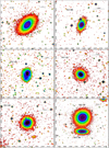 |
Fig. A.1 Digitized Sky Survey images of the F3D galaxies. For each galaxy, the 1 × 1 arcmin2 MUSE pointings are shown in black. The black dashed ellipse corresponds to the isophote at μB = 25 mag arcsec−2. The right ascension and declination (J2000.0) are given in degrees on the horizontal and vertical axes of the field of view, respectively. |
References
- Alabi, A. B., Forbes, D. A., Romanowsky, A. J., et al. 2017, MNRAS, 468, 3949 [NASA ADS] [CrossRef] [Google Scholar]
- Arnold, J. A., Romanowsky, A. J., Brodie, J. P., et al. 2014, ApJ, 791, 80 [NASA ADS] [CrossRef] [Google Scholar]
- Bacon, R., Accardo, M., Adjali, L., et al. 2010, in Ground-based and Airborne Instrumentation for Astronomy III, Proc. SPIE, 7735, 773508 [Google Scholar]
- Bahcall, N. A., & Cen, R. 1993, ApJ, 407, L49 [NASA ADS] [CrossRef] [Google Scholar]
- Baldwin, J. A., Phillips, M. M., & Terlevich, R. 1981, PASP, 93, 5 [NASA ADS] [CrossRef] [EDP Sciences] [Google Scholar]
- Bedregal, A. G., Aragón-Salamanca, A., Merrifield, M. R., & Milvang-Jensen, B. 2006, MNRAS, 371, 1912 [NASA ADS] [CrossRef] [Google Scholar]
- Bellstedt, S., Forbes, D. A., Romanowsky, A. J., et al. 2018, MNRAS, 476, 4543 [NASA ADS] [CrossRef] [Google Scholar]
- Blakeslee, J. P., Jordán, A., Mei, S., et al. 2009, ApJ, 694, 556 [NASA ADS] [CrossRef] [Google Scholar]
- Blasquez, P., Peletier, R. F., Jimenez-Vicente, J., et al. 2006, MNRAS, 371, 703 [NASA ADS] [CrossRef] [Google Scholar]
- Boardman, N. F., Weijmans, A.-M., van den Bosch, R., et al. 2017, MNRAS, 471, 4005 [NASA ADS] [CrossRef] [Google Scholar]
- Bois, M., Emsellem, E., Bournaud, F., et al. 2011, MNRAS, 416, 1654 [NASA ADS] [CrossRef] [Google Scholar]
- Brodie, J. P., Romanowsky, A. J., Strader, J., et al. 2014, ApJ, 796, 52 [NASA ADS] [CrossRef] [Google Scholar]
- Bundy, K., Bershady, M. A., Law, D. R., et al. 2015, ApJ, 798, 7 [NASA ADS] [CrossRef] [Google Scholar]
- Buzzoni, A., Arnaboldi, M., & Corradi, R. L. M. 2006, MNRAS, 368, 877 [NASA ADS] [CrossRef] [Google Scholar]
- Caon, N., Capaccioli, M., & D’Onofrio, M. 1994, A&AS, 106, 199 [NASA ADS] [Google Scholar]
- Cappellari, M. 2002, MNRAS, 333, 400 [NASA ADS] [CrossRef] [Google Scholar]
- Cappellari, M. 2016, ARA&A, 54, 597 [NASA ADS] [CrossRef] [Google Scholar]
- Cappellari, M. 2017, MNRAS, 466, 798 [NASA ADS] [CrossRef] [Google Scholar]
- Cappellari, M., & Copin, Y. 2003, MNRAS, 342, 345 [NASA ADS] [CrossRef] [Google Scholar]
- Cappellari, M., & Emsellem, E. 2004, PASP, 116, 138 [NASA ADS] [CrossRef] [Google Scholar]
- Cappellari, M., Emsellem, E., Krajnović, D., et al. 2011, MNRAS, 413, 813 [NASA ADS] [CrossRef] [Google Scholar]
- Cappellari, M., McDermid, R. M., Alatalo, K., et al. 2013, MNRAS, 432, 1862 [NASA ADS] [CrossRef] [Google Scholar]
- Catinella, B., Schiminovich, D., Cortese, L., et al. 2013, MNRAS, 436, 34 [NASA ADS] [CrossRef] [Google Scholar]
- Choi, J., Conroy, C., Moustakas, J., et al. 2014, ApJ, 792, 95 [NASA ADS] [CrossRef] [Google Scholar]
- Ciardullo, R., Jacoby, G. H., Ford, H. C., & Neill, J. D. 1989, ApJ, 339, 53 [NASA ADS] [CrossRef] [Google Scholar]
- Coccato, L., Fabricius, M., Morelli, L., et al. 2015, A&A, 581, A65 [NASA ADS] [CrossRef] [EDP Sciences] [Google Scholar]
- Conroy, C., Graves, G. J., & van Dokkum P. G. 2014, ApJ, 780, 33 [NASA ADS] [CrossRef] [Google Scholar]
- Croom, S. M., Lawrence, J. S., Bland-Hawthorn, J., et al. 2012, MNRAS, 421, 872 [NASA ADS] [Google Scholar]
- Davis, T. A., Alatalo, K., Sarzi, M., et al. 2011, MNRAS, 417, 882 [NASA ADS] [CrossRef] [Google Scholar]
- de Vaucouleurs, G., de Vaucouleurs, A., Corwin, Jr. H. G., et al. 1991, Third Reference Catalogue of Bright Galaxies (New York, NY: Springer) [Google Scholar]
- de Zeeuw, P. T., Bureau, M., Emsellem, E., et al. 2002, MNRAS, 329, 513 [NASA ADS] [CrossRef] [Google Scholar]
- Drinkwater, M. J., Gregg, M. D., & Colless, M. 2001, ApJ, 548, L139 [NASA ADS] [CrossRef] [Google Scholar]
- Duc, P.-A., Cuillandre, J.-C., Karabal, E., et al. 2015, MNRAS, 446, 120 [NASA ADS] [CrossRef] [Google Scholar]
- Dutton, A. A., & Macciò, A. V. 2014, MNRAS, 441, 3359 [NASA ADS] [CrossRef] [Google Scholar]
- Emsellem, E., Monnet, G., & Bacon, R. 1994, A&A, 285, 723 [NASA ADS] [Google Scholar]
- Emsellem, E., Cappellari, M., Krajnović, D., et al. 2007, MNRAS, 379, 401 [NASA ADS] [CrossRef] [Google Scholar]
- Emsellem, E., Cappellari, M., Krajnović, D., et al. 2011, MNRAS, 414, 888 [NASA ADS] [CrossRef] [Google Scholar]
- Emsellem, E., Krajnović, D., & Sarzi, M. 2014, MNRAS, 445, L79 [NASA ADS] [CrossRef] [Google Scholar]
- Erwin, P. 2015, ApJ, 799, 226 [NASA ADS] [CrossRef] [Google Scholar]
- Falcón-Barroso, J., Bacon, R., Bureau, M., et al. 2006, MNRAS, 369, 529 [NASA ADS] [CrossRef] [Google Scholar]
- Falcón-Barroso, J., Lyubenova, M., van de Ven, G., et al. 2017, A&A, 597, A48 [NASA ADS] [CrossRef] [EDP Sciences] [Google Scholar]
- Ferguson, H. C., & Sandage, A. 1989, AJ, 98, 367 [Google Scholar]
- Foster, C., Pastorello, N., Roediger, J., et al. 2016, MNRAS, 457, 147 [NASA ADS] [CrossRef] [Google Scholar]
- Foster, C., van de Sande, J., D’Eugenio, F., et al. 2017, MNRAS, 472, 966 [NASA ADS] [CrossRef] [Google Scholar]
- Freudling, W., Romaniello, M., Bramich, D. M., et al. 2013, A&A, 559, A96 [NASA ADS] [CrossRef] [EDP Sciences] [Google Scholar]
- Gadotti, D. A., Seidel, M. K., Sánchez-Blázquez, P., et al. 2015, A&A, 584, A90 [NASA ADS] [CrossRef] [EDP Sciences] [Google Scholar]
- García-Benito, R., Zibetti, S., Sánchez, S. F., et al. 2015, A&A, 576, A135 [NASA ADS] [CrossRef] [EDP Sciences] [Google Scholar]
- González, J. J. 1993, PhD Thesis, University of California, Santa Cruz [Google Scholar]
- Greene, J. E., Janish, R., Ma, C.-P., et al. 2015, ApJ, 807, 11 [NASA ADS] [CrossRef] [Google Scholar]
- Guérou, A., Emsellem, E., Krajnović, D., et al. 2016, A&A, 591, A143 [NASA ADS] [CrossRef] [EDP Sciences] [Google Scholar]
- Hirschmann, M., Naab, T., Ostriker, J. P., et al. 2015, MNRAS, 449, 528 [NASA ADS] [CrossRef] [Google Scholar]
- Iodice, E., Coccato, L., Combes, F., et al. 2015, A&A, 583, A48 [NASA ADS] [CrossRef] [EDP Sciences] [Google Scholar]
- Iodice, E., Capaccioli, M., Grado, A., et al. 2016, ApJ, 820, 42 [NASA ADS] [CrossRef] [Google Scholar]
- Iodice, E., Spavone, M., Capaccioli, M., et al. 2017, ApJ, 839, 21 [NASA ADS] [CrossRef] [Google Scholar]
- Janowiecki, S., Mihos, J. C., Harding, P., et al. 2010, ApJ, 715, 972 [NASA ADS] [CrossRef] [Google Scholar]
- Johnston, E. J., Merrifield, M. R., Aragón-Salamanca, A., & Cappellari, M. 2013, MNRAS, 428, 1296 [NASA ADS] [CrossRef] [Google Scholar]
- Jordán, A., Blakeslee, J. P., Côté, P., et al. 2007, ApJS, 169, 213 [NASA ADS] [CrossRef] [Google Scholar]
- Jordán, A., Peng, E. W., Blakeslee, J. P., et al. 2015, ApJS, 221, 13 [NASA ADS] [CrossRef] [Google Scholar]
- Keel, W. C., Lintott, C. J., Schawinski, K., et al. 2012, AJ, 144, 66 [NASA ADS] [CrossRef] [Google Scholar]
- Kennicutt, Jr. R. C. 1998, ApJ, 498, 541 [NASA ADS] [CrossRef] [Google Scholar]
- Krajnović, D., Alatalo, K., Blitz, L., et al. 2013, MNRAS, 432, 1768 [NASA ADS] [CrossRef] [Google Scholar]
- Krajnović, D., Weilbacher, P. M., Urrutia, T., et al. 2015, MNRAS, 452, 2 [NASA ADS] [CrossRef] [Google Scholar]
- La Barbera, F., Vazdekis, A., Ferreras, I., et al. 2017, MNRAS, 464, 3597 [NASA ADS] [CrossRef] [Google Scholar]
- Lyubenova, M., Martín-Navarro, I., van de Ven, G., et al. 2016, MNRAS, 463, 3220 [NASA ADS] [CrossRef] [Google Scholar]
- Martín-Navarro, I., La Barbera, F., Vazdekis, A., Falcón-Barroso, J., & Ferreras, I. 2015, MNRAS, 447, 1033 [NASA ADS] [CrossRef] [Google Scholar]
- McConnell, N. J., Lu, J. R., & Mann, A. W. 2016, ApJ, 821, 39 [NASA ADS] [CrossRef] [Google Scholar]
- McDermid, R. M., Alatalo, K., Blitz, L., et al. 2015, MNRAS, 448, 3484 [NASA ADS] [CrossRef] [Google Scholar]
- Mentz, J. J., La Barbera, F., Peletier, R. F., et al. 2016, MNRAS, 463, 2819 [NASA ADS] [CrossRef] [Google Scholar]
- Mihos, J. C., Harding, P., Feldmeier, J., & Morrison, H. 2005, ApJ, 631, L41 [NASA ADS] [CrossRef] [Google Scholar]
- Naab, T., Oser, L., Emsellem, E., et al. 2014, MNRAS, 444, 3357 [NASA ADS] [CrossRef] [Google Scholar]
- Navarro, J. F., Frenk, C. S., & White, S. D. M. 1997, ApJ, 490, 493 [NASA ADS] [CrossRef] [Google Scholar]
- Noll, S., Kausch, W., Kimeswenger, S., et al. 2014, A&A, 567, A25 [NASA ADS] [CrossRef] [EDP Sciences] [Google Scholar]
- Odekon, M. C., Koopmann, R. A., Haynes, M. P., et al. 2016, ApJ, 824, 110 [NASA ADS] [Google Scholar]
- Oh, K., Sarzi, M., Schawinski, K., & Yi, S. K. 2011, ApJS, 195, 13 [NASA ADS] [CrossRef] [Google Scholar]
- Oldham, L., & Auger, M. 2018, MNRAS, 474, 4169 [NASA ADS] [CrossRef] [Google Scholar]
- Pastorello, N., Sarzi, M., Cappellari, M., et al. 2013, MNRAS, 430, 1219 [NASA ADS] [CrossRef] [Google Scholar]
- Pastorello, N., Forbes, D. A., Foster, C., et al. 2014, MNRAS, 442, 1003 [NASA ADS] [CrossRef] [Google Scholar]
- Peng, C. Y., Ho, L. C., Impey, C. D., & Rix, H.-W. 2010, AJ, 139, 2097 [NASA ADS] [CrossRef] [Google Scholar]
- Pinna, F., Falcón-Barroso, J., Martig, M., et al. 2018, A&A, submitted [Google Scholar]
- Poci, A., Cappellari, M., & McDermid, R. M. 2017, MNRAS, 467, 1397 [NASA ADS] [Google Scholar]
- Sánchez, S. F., Kennicutt, R. C., Gil de Paz, A., et al. 2012, A&A, 538, A8 [NASA ADS] [CrossRef] [EDP Sciences] [Google Scholar]
- Sarzi, M., Falcón-Barroso, J., Davies, R. L., et al. 2006, MNRAS, 366, 1151 [NASA ADS] [CrossRef] [Google Scholar]
- Sarzi, M., Mamon, G. A., Cappellari, M., et al. 2011, MNRAS, 415, 2832 [NASA ADS] [CrossRef] [Google Scholar]
- Sarzi, M., Spiniello, C., La Barbera, F., Krajnović, D., & van den Bosch, R. 2018, MNRAS, 478, 4084 [NASA ADS] [CrossRef] [Google Scholar]
- Schmidt, M. 1959, ApJ, 129, 243 [NASA ADS] [CrossRef] [Google Scholar]
- Scott, N., Davies, R. L., Houghton, R. C. W., et al. 2014, MNRAS, 441, 274 [NASA ADS] [CrossRef] [Google Scholar]
- Smette, A., Sana, H., Noll, S., et al. 2015, A&A, 576, A77 [NASA ADS] [CrossRef] [EDP Sciences] [Google Scholar]
- Smith, R. J. 2014, MNRAS, 443, L69 [NASA ADS] [CrossRef] [Google Scholar]
- Soto, K. T., Lilly, S. J., Bacon, R., Richard, J., & Conseil, S. 2016, MNRAS, 458, 3210 [NASA ADS] [CrossRef] [Google Scholar]
- Spavone, M., Capaccioli, M., Napolitano, N. R., et al. 2017, A&A, 603, A38 [NASA ADS] [CrossRef] [EDP Sciences] [Google Scholar]
- Spiniello, C., Trager, S., Koopmans, L. V. E., & Conroy, C. 2014, MNRAS, 438, 1483 [NASA ADS] [CrossRef] [Google Scholar]
- Spiniello, C., Napolitano, N. R., Arnaboldi, M., et al. 2018, MNRAS, 477, 1880 [NASA ADS] [CrossRef] [Google Scholar]
- Stetson, P. B. 1987, PASP, 99, 191 [NASA ADS] [CrossRef] [Google Scholar]
- Treu, T., Auger, M. W., Koopmans, L. V. E., et al. 2010, ApJ, 709, 1195 [NASA ADS] [CrossRef] [Google Scholar]
- van den Bosch, R. C. E., van de Ven, G., Verolme, E. K., Cappellari, M., & de Zeeuw P. T. 2008, MNRAS, 385, 647 [NASA ADS] [CrossRef] [Google Scholar]
- van Dokkum, P. G., & Conroy, C. 2010, Nature, 468, 940 [NASA ADS] [CrossRef] [Google Scholar]
- van Dokkum, P., Conroy, C., Villaume, A., Brodie, J., & Romanowsky, A. J. 2017, ApJ, 841, 68 [NASA ADS] [CrossRef] [Google Scholar]
- Vazdekis, A., Sánchez-Blázquez, P., Falcón-Barroso, J., et al. 2010, MNRAS, 404, 1639 [NASA ADS] [Google Scholar]
- Vazdekis, A., Ricciardelli, E., Cenarro, A. J., et al. 2012, MNRAS, 424, 157 [NASA ADS] [CrossRef] [Google Scholar]
- Venhola, A., Peletier, R., Laurikainen, E., et al. 2017, A&A, 608, A142 [NASA ADS] [CrossRef] [EDP Sciences] [Google Scholar]
- Weijmans, A.-M., Cappellari, M., Bacon, R., et al. 2009, MNRAS, 398, 561 [NASA ADS] [CrossRef] [Google Scholar]
- Weijmans, A.-M., de Zeeuw, P. T., Emsellem, E., et al. 2014, MNRAS, 444, 3340 [NASA ADS] [CrossRef] [Google Scholar]
- Weilbacher, P. M., Streicher, O., Urrutia, T., et al. 2012, in Software and Cyberinfrastructure for Astronomy II, Proc. SPIE, 8451, 84510B [NASA ADS] [CrossRef] [Google Scholar]
- Weilbacher, P. M., Streicher, O., & Palsa, R. 2016, MUSE-DRP: MUSE Data Reduction Pipeline, Astrophysics Source Code Library [record ascl:1610.004] [Google Scholar]
- Zhu, L., van den Bosch, R., van de Ven, G., et al. 2018, MNRAS, 473, 3000 [NASA ADS] [CrossRef] [Google Scholar]
- Zieleniewski, S., Houghton, R. C. W., Thatte, N., & Davies, R. L. 2015, MNRAS, 452, 597 [NASA ADS] [CrossRef] [Google Scholar]
The Image Reduction and Analysis Facility is distributed by the National Optical Astronomy Observatory (NOAO), which is operated by the Association of Universities for Research in Astronomy (AURA), Inc. under cooperative agreement with the National Science Foundation.
All Tables
All Figures
|
Fig. 1 Location on the sky of the ETGs (circles) and LTGs (crosses) with mB < 15 mag in the Fornax cluster. The dashed circle marks the virial radius of the cluster and corresponds to about 0.7 Mpc, as determined by Drinkwater et al. (2001). The red symbols show F3D galaxies while the blue symbols correspond to NGC 1316 (filled circle) and NGC 1365 (cross) for which MUSE data are already available in the ESO Science Archive Facility. |
| In the text | |
|
Fig. 2 Left panel: spatial coverage of the MUSE central pointings of the F3D ETGs in units of 30 arcsec ∕Re (histogram) compared to the ATLAS3D (Cappellari et al. 2011; dotted line) and MaNGA (Bundy et al. 2015; primary sample: dashed line, secondary sample: dash-dotted line) surveys. Right panel: spatial coverage of the MUSE halo pointings of the F3D ETGs down to μB = 25 mag arcsec−2 in units of R25∕Re (histogram) compared to the MASSIVE (Greene et al. 2015, dotted line) and SLUGGS (Foster et al. 2016, dashed line) surveys. |
| In the text | |
|
Fig. 3 r-Band image of FCC 167 from the Fornax Deep Survey with VST (Iodice et al. 2016; Venhola et al. 2017). The 1 × 1 arcmin2 MUSE pointings are shown in black. The black dashed ellipse corresponds to the isophote at μB = 25 mag arcsec−2, while the right ascension and declination (J2000.0) are given in degrees on the horizontal and vertical axes of the field of view, respectively. |
| In the text | |
|
Fig. 4 Top panel: MUSE reconstructed image of the combined mosaic of FCC 167 compared with isophotes of the r-band VST image shown in Fig. 3. The black isophotes cover the range between μr = 16.6 and 22.6 mag arcsec−2 and are spaced by 1 mag arcsec−2. The grey isophote corresponds to μB = 25 mag arcsec−2. The blue and orange circles indicate, respectively, the position of the central and outer apertures selected for testing the spectral quality of the F3D data (see Fig. 5). The red dashed lines mark the 2 arcsec wide aperture along the galaxy major axis (P.A. = 3.9°) where the surface-brightness radial profile plotted in the bottom panel was extracted. Bottom panel: surface-brightness radial profile along the major axis of FCC 167 from the MUSE reconstructed image (red points) and r-band VST image (black points). The sky level of MUSE (horizontal continuous line) and μB = 25 mag arcsec−2 (horizontal dashed line) are shown for comparison. |
| In the text | |
|
Fig. 5 GandALF fits to the central (top panel) and outer aperture (bottom panel) spectra extracted from the MUSE data of FCC 167 (see Fig. 4). To allow a more direct comparison between these two spectra (black lines) and their respective GandALF fits (green and red lines), both data and models were normalised and rescaled. The residuals obtained by subtracting the model from the spectrum are also shown (bluepoints). These models used the entire MILES (Blasquez et al. 2006) stellar library as stellar templates to achieve the best possible fit. At the same time, to ensure a physically-motivated model only reddening by dust was used to adjust the templates to the observed shape of the stellar continuum. The position of the most prominent [O I] sky emission lines is indicated. |
| In the text | |
|
Fig. 6 Top panel: quality of the Voronoi-binned spectra for a target S∕N = 40 as a functionof r-band surface brightness in MUSE data of FCC 167. The S/rN ratio between the median value of the flux and the noise level in the fit residuals is used as a more conservative measure of the spectral quality. Lower panel: level of spatial correlation in the MUSE data of FCC 167. The covariance ratio β = rN∕N between the fit residual noise and the formally propagated noise increases as function of bin size (or number ofspaxels) in each Voronoi bin, although much less than in the CALIFA data (blue line). The β trend is well described by a quadratic form in logNspaxels (red line). |
| In the text | |
|
Fig. 7 Stellar kinematic maps of the mean velocity v, velocity dispersion σ, and higher-order moments h3 and h4 of the line-of-sight velocity distribution for FCC 167 derived from the S∕N = 40 Voronoi-binned MUSE data with the r-band isophotes (black lines) shown in Fig. 4. |
| In the text | |
|
Fig. 8 Best-fitting Schwarzschild orbit-based dynamical model of FCC 167. Top and middle panels: observed and best-fitting model of the surface brightness SB, mean velocity v, velocity dispersion σ, and higher-order moments h3 and h4 of the line-of-sight velocity distribution, respectively. Bottom panels: residuals obtained by subtracting the best-fitting model from data. |
| In the text | |
|
Fig. 9 Orbital and photometric decomposition of FCC 167. Left panel: orbit distribution in the phase space of circularity λZ vs. intrinsic radius r, as derived from the best-fitting orbit-superposition model shown in Fig. 8. Grey-scale colours indicate the orbital density in phase space. The horizontal dashed lines separate stars in highly-circular cold thin-disc orbits (λZ > 0.7) from those following dynamically warm thick-disc motions (0.2 < λZ < 0.7) and those in the non-rotating bulge and stellar halo (λZ ~ 0). Right panel:stellar surface-density profiles of FCC 167. The grey lines trace the profiles of a classical exponential disc and Sérsic bulge as derived from a standard bulge-disc decomposition, whereas the blue, orange, and red lines follow the projected surface brightness of the dynamically cold, warm (thick disc), and hot (bulge) components, respectively. |
| In the text | |
|
Fig. 10 Two-dimensional light distribution for the dynamical and photometric components of FCC 167. Left panel: two-dimensional distribution of light from each of the dynamical components, as derived from the best-fitting orbit-superposition model shown in Fig. 8: dynamically cold, warm (thick disc), and hot (bulge) componentsare shown in the top, middle and lower panel, respectively. Right panel: two-dimensional distribution of light from each of the photometric components, Sérsic bulge (middle panel) and exponential disc (top panel), as derived from the fit of the light distribution of the MUSE reconstructed image shown in Fig. 4. In the lower panel is shown the resulting image from the superposition of the hot (bulge) and warm (thick disc) dynamical components. In all panels, the colour bar indicates the surface brightness levels adopting an arbitrary zero point. |
| In the text | |
|
Fig. 11 Stellar kinematics of FCC 167 extracted from the MUSE data (black points) at P.A. = 3.9° within the2 arcsec wide aperture crossing the nucleus shown in Fig. 4. The mean velocity v (bottom panel) and velocity dispersion σ (top panel) are given. The mean errors of the data are shown in the lower-right corner of each panel. The velocity dispersion is compared to the long-slit spectroscopic data obtained by Bedregal et al. (2006) for the north side of the galaxy (red points). The vertical dashed line corresponds to the effective radius. |
| In the text | |
|
Fig. 12 High-frequency residual image obtained from the r-band VST image of FCC 167. The 1 × 1 arcmin2 MUSE pointings are overplotted in black. The black dashed lines mark the 2 arcsec wide aperture at P.A. = 3.9°, where the stellar kinematics shown in Fig. 11 was extracted from the MUSE data. The right ascension and declination (J2000.0) are given in degrees on the vertical and horizontal axes of the field of view, respectively. |
| In the text | |
|
Fig. 13 Mg b map of FCC 167 with the r-band isophotes (black lines) and B-band isophote (grey line) shown in Fig. 4. The orange and red circles indicate the location of two selected apertures where the Hβ, Mg b, Fe5270, Fe5335, and Fe5406 line-strength indices were measured and fitted in order to constrain the stellar population properties, as shown in Fig. 14. |
| In the text | |
|
Fig. 14 Stellar population properties from the two selected apertures in the middle (left panels) and halo pointing (right panels) of FCC 167 shown in Fig. 13. Top panels: rest-frame spectra (black lines), best-fitting models (red lines), and residuals obtained by subtracting models from spectra (green points). Bottom panels: posterior distributions for the age, metallicity [M/H], and α-element abundance [Mg/Fe]. The dashed lines overplotted on the histograms indicate the 16%, 50%, and 84% percentiles of the marginalised distributions. |
| In the text | |
|
Fig. 15 Illustration of GC extraction from MUSE data of FCC 167. Top panel: residual image obtained by subtractingthe IMFIT surface-brightness model of FCC 167 from the galaxy surface-brightness distribution extracted from MUSE data. The GC candidates from MUSE data (blue circles) and GCs in the HST/ACS GC catalogue (Jordán et al. 2015; red crosses) are shown. Middle panel: map of the mean stellar velocity of FCC 167 shown in Fig. 8 and radial velocities of the GCs. Bottom panel: spectra of two MUSE GCs with S∕N ≈ 25 (purple line) and 5 (green line) whose location is indicated in the top panel by the filled purple and open green triangles, respectively. |
| In the text | |
|
Fig. 16 Map of the flux of the [O III]λ5007 emission from the central pointing of FCC 167. The extended disc is clearly visible. The detected planetary nebulae are indicated by red circles. [O III]λ5007 flux values are shown on a logarithmic scale and in 10−20 erg cm−2 s−1. |
| In the text | |
|
Fig. 17 Digitized Sky Survey image of FCC 312. The 1 × 1 arcmin2 MUSE pointings are shown in black. The black dashed ellipse corresponds to the isophote at μB = 25 mag arcsec−2, while the right ascension and declination (J2000.0) are given in degrees on the horizontal and vertical axes of the field of view, respectively. |
| In the text | |
|
Fig. 18 Emission-line analysis for the central regions of FCC 312. Top panels: maps of the total flux, mean velocity and velocity dispersion along the line-of-sight from the [N II]λ6583 nebular emission. Middle panels: maps of the [N II]λ6583/Hα and [O III]λ5007/Hβ line ratios and corresponding BPT diagram. Bottom panels: maps of the de-reddened Hα flux, extinction on the nebular lines, and extinction derived from the stellar continuum. Velocities and velocity dispersions are in km s−1, reddening values are in magnitude, line ratios and fluxes are shown in a logarithmic scales, with the latter in units of 10−20 erg cm−2 s−1. Grey areas in the maps refer to regions where the S/N of the relevant lines was not sufficiently elevated to firmly exclude a false positive detection. These levels were established in regions devoid of emission well above and below the equatorial plane of the galaxy. |
| In the text | |
|
Fig. 19 Correlation between the dust extinction affecting nebular lines and Hα luminosity in the same region, corrected for total extinction. Regions with elevated star formation rate are also heavily dust obscured. |
| In the text | |
|
Fig. A.1 Digitized Sky Survey images of the F3D galaxies. For each galaxy, the 1 × 1 arcmin2 MUSE pointings are shown in black. The black dashed ellipse corresponds to the isophote at μB = 25 mag arcsec−2. The right ascension and declination (J2000.0) are given in degrees on the horizontal and vertical axes of the field of view, respectively. |
| In the text | |
Current usage metrics show cumulative count of Article Views (full-text article views including HTML views, PDF and ePub downloads, according to the available data) and Abstracts Views on Vision4Press platform.
Data correspond to usage on the plateform after 2015. The current usage metrics is available 48-96 hours after online publication and is updated daily on week days.
Initial download of the metrics may take a while.