| Issue |
A&A
Volume 663, July 2022
|
|
|---|---|---|
| Article Number | A135 | |
| Number of page(s) | 21 | |
| Section | Extragalactic astronomy | |
| DOI | https://doi.org/10.1051/0004-6361/202243290 | |
| Published online | 20 July 2022 | |
Fornax3D project: Assembly history of massive early-type galaxies in the Fornax cluster from deep imaging and integral field spectroscopy
1
INAF–Osservatorio Astronomico di Capodimonte, Salita Moiariello 16, 80131 Napoli, Italy
e-mail: This email address is being protected from spambots. You need JavaScript enabled to view it.
2
Instituto de Astrofísica, Facultad de Física, Pontificia Universidad Católica de Chile, Casilla 306, Santiago 22, Chile
3
Department of Astrophysics, University of Vienna, Tuerkenschanzstrasse 17, 1180 Vienna, Austria
4
Instituto de Astronomía y Ciencias Planetarias, Avenida Copayapu 485, Copiapó, Chile
5
Dipartimento di Fisica e Astronomia “G. Galilei”, Universitá di Padova, vicolo dell’Osservatorio 3, 35122 Padova, Italy
6
INAF–Osservatorio Astronomico di Padova, visolo dell’Osservatorio 5, 35122 Padova, Italy
7
Armagh Observatory and Planetarium, College Hill, Armagh BT61 9DG, UK
8
European Southern Observatory, Karl-Schwarzschild-Strasse 2, 85748 Garching bei Muenchen, Germany
9
European Space Agency, European Space Research and Technology Centre, Keplerlaan 1, 2200 AG Noordwijk, The Netherlands
10
Instituto de Astrofísica de Canarias, Vía Láctea s/n, 38205 La Laguna, Tenerife, Spain
11
Departamento de Astrofísica, Universidad de La Laguna, 38200 La Laguna, Tenerife, Spain
12
Research Centre for Astronomy, Astrophysics, and Astrophotonics, Department of Physics and Astronomy, Macquarie University, Sydney, NSW 2109, Australia
13
Max-Planck-Institut fuer Astronomie, Koenigstuhl 17, 69117 Heidelberg, Germany
14
Centre for Extragalactic Astronomy, University of Durham, Stockton Road, Durham DH1 3LE, UK
15
Sterrewacht Leiden, Leiden University, Postbus 9513, 2300 RA Leiden, The Netherlands
16
Max-Planck-Institut fuer extraterrestrische Physik, Giessenbachstrasse 1, 85748 Garching bei Muenchen, Germany
17
Shanghai Astronomical Observatory, Chinese Academy of Sciences, 80 Nandan Road, Shanghai 200030, PR China
Received:
9
February
2022
Accepted:
27
May
2022
Abstract
This work is based on high-quality integral-field spectroscopic data obtained with the Multi Unit Spectroscopic Explorer (MUSE) on the Very Large Telescope (VLT). The 21 brightest (mB ≤ 15 mag) early-type galaxies (ETGs) inside the virial radius of the Fornax cluster are observed out to distances of ∼2−3 Re. Deep imaging from the VLT Survey Telescope (VST) is also available for the sample ETGs. We investigated the variation of the galaxy structural properties as a function of the total stellar mass and cluster environment. Moreover, we correlated the size scales of the luminous components derived from a multi-component decomposition of the VST surface-brightness radial profiles of the sample ETGs with the MUSE radial profiles of stellar kinematic and population properties. The results are compared with both theoretical predictions and previous observational studies and used to address the assembly history of the massive ETGs of the Fornax cluster. We find that galaxies in the core and north-south clump of the cluster, which have the highest accreted mass fraction, show milder metallicity gradients in their outskirts than the galaxies infalling into the cluster. We also find a segregation in both age and metallicity between the galaxies belonging to the core and north-south clump and the infalling galaxies. The new findings fit well within the general framework for the assembly history of the Fornax cluster.
Key words: galaxies: elliptical and lenticular, cD / galaxies: evolution / galaxies: formation / galaxies: kinematics and dynamics / galaxies: photometry / galaxies: structure
© M. Spavone et al. 2022
 Open Access article, published by EDP Sciences, under the terms of the Creative Commons Attribution License (https://creativecommons.org/licenses/by/4.0), which permits unrestricted use, distribution, and reproduction in any medium, provided the original work is properly cited.
This article is published in open access under the Subscribe-to-Open model. This email address is being protected from spambots. You need JavaScript enabled to view it. to support open access publication.
1. Introduction
The Λ cold dark matter (ΛCDM) theory for galaxy formation predicts that galaxies grow through a combination of in situ star formation and accretion of stars from other galaxies (White & Frenk 1991). In this respect, mapping the outer structure of galaxies down to low stellar surface-brightness levels is crucial to constraining their evolution within the ΛCDM paradigm. Indeed, the dynamical timescales in the outskirts of galaxies are very long (typically of the order of several gigayears (Gyrs)), so that the properties of the stellar halos can be used as a fossil record of the past galactic interactions. In particular, the structural properties of the outer regions of galaxies and their correlation with the stellar mass and other observables (e.g., stellar kinematics and population properties) might therefore provide ways of testing theoretical predictions of growth by accretion.
Measuring the surface-brightness radial profiles of early-type galaxies (ETGs) out to the faintest levels turned out to be one of the main ‘tools’ to quantify the amount of the accreted mass. This method becomes particularly efficient when the stars of the outer stellar envelope are dominant (e.g., Gonzalez et al. 2005; Seigar et al. 2007; Kormendy et al. 2009; Trujillo & Fliri 2016; Iodice et al. 2016; Kluge et al. 2020; Spavone et al. 2020). Deep photometric images are therefore needed to set the size scales of the main galaxy components.
In turn, the stellar kinematics and population properties from the integrated light (e.g., Coccato et al. 2010, 2011; Ma et al. 2014; Barbosa et al. 2018; Veale et al. 2018; Greene et al. 2019) and kinematics of discrete tracers such as globular clusters (GCs) and planetary nebulae (PNe) (e.g., Coccato et al. 2013; Longobardi et al. 2013; Forbes 2017; Spiniello et al. 2018; Hartke et al. 2018; Fahrion et al. 2020a,b) have also been used to trace the mass assembly in the outer regions of galaxies. The presence of stellar population gradients from the centre out to the stellar halo and the different PN and GC kinematics at different radii are indicative of a different star formation history in the central in situ component with respect to that of the galaxy outskirts (e.g., Greene et al. 2015; McDermid et al. 2015; Martín-Navarro et al. 2015; Barone et al. 2018; Ferreras et al. 2019).
Since the study of the outskirts of galaxies is a challenging task due to their low surface-brightness level, the comparison between the photometric and spectroscopic observables and the theoretical predictions has not provided a general consensus yet. Both N-body and hydrodynamical simulations predict that the amount of accreted mass (i.e. the ex situ component) is a function of the total stellar mass of a galaxy, with the higher mass galaxies having an higher accreted mass fraction (Cooper et al. 2013; Pillepich et al. 2018; Schulze et al. 2020). Furthermore, the surface-brightness and metallicity radial profiles appear flatter in the galaxy outskirts when repeated mergers occur (Cook et al. 2016), suggesting that the accreted fraction of metal-rich stars increases. By analysing the Magneticum Pathfinder simulations, Schulze et al. (2020) discovered that the radius marking the kinematic transition between different galaxy components provides a good estimate of the transition radius between the in situ and accreted component. In contrast, using Illustris TNG100 simulations Pulsoni et al. (2020) found that the kinematic transition radius does not generally correspond to the transition radius between the regions dominated by the in situ and ex situ components. Recently, Remus & Forbes (2021) pointed out that the accreted mass fraction derived from the fit of the surface-brightness radial profiles seems to be a lower limit of the total accreted mass during the growth process. To address the above open issues it would be very valuable to i) correlate the size scales of the different galaxy components derived from deep photometry with the kinematic and stellar population properties out to comparable radii and low surface-brightness levels and ii) compare these findings with available theoretical predictions.
To date, the deep images from the Fornax Deep Survey (FDS, Iodice et al. 2016; Venhola et al. 2017) and integral-field spectroscopy from the Fornax 3D project (F3D, Sarzi et al. 2018), available for a large sample of galaxies in the Fornax cluster, offer a unique opportunity to perform the combined analysis mentioned above. This is the primary goal of the present paper. In detail, we explored the mass assembly history of the ETGs in the Fornax cluster by teaming deep photometry, which traces the galaxy structure out to the stellar halo region, with kinematics and stellar populations, which are measured outside the transition radius from the in situ to ex situ components.
The emerging picture of the Fornax cluster from the FDS and F3D surveys (Iodice et al. 2019a,b; Spavone et al. 2020; Napolitano et al. 2022) suggests that the assembly of the cluster is ongoing, in agreement with earlier findings by Drinkwater et al. (2001) and Scharf et al. (2005). Based on the analysis of the projected phase space, Iodice et al. (2019a) proposed that the cluster is made of three well-defined sub-structures of galaxies: the core, the north-south clump (NS-clump), and the infalling galaxies. In addition, there is the southwest group of galaxies centred around NGC 1316, which is falling into the cluster potential (Drinkwater et al. 2001). The galaxies of each sub-structure have different morphologies, colours, accreted mass fractions, kinematics, and stellar populations.
The core is dominated by the brightest and most massive cluster members, NGC 1399 and NGC 1404, which also coincides with the peak of the X-ray emission (Paolillo et al. 2002). The NS clump includes all the reddest and most metal-rich galaxies of the sample, with stellar masses in the (0.3−9.8) × 1010 M⊙ range. The core and NS clump reside in the high-density region of the cluster (at a cluster-centric distance of Rproj ≤ 0.4Rvir ∼ 0.3 Mpc), where the X-ray emission dominates. The brightest ETGs in these groups have the largest accreted mass fraction (∼70−80%), constrained by fitting the light distribution out the stellar halo region (i.e. down to a surface brightness level of μg ∼ 28−30 mag arcsec−2; Spavone et al. 2020). In this region of the cluster, diffuse intra-cluster light (ICL) was detected on the west side of the core, where the NS clump is located (Iodice et al. 2017). The intra-cluster GCs and PNe were found to be associated with the ICL (Spiniello et al. 2018; Cantiello et al. 2020; Chaturvedi et al. 2022).
The infalling galaxies appear to be nearly symmetrically distributed in projection around the core. They populate the low-density region of the cluster, at Rproj ≥ 0.4Rvir ∼ 0.3 Mpc. They are bluer and less massive (∼109 − 1010 M⊙) than the galaxies in the core and NS clump (Iodice et al. 2019b). The majority of them are late-type galaxies (LTGs), with ongoing star formation and a disturbed morphology (in the form of tidal tails and disturbed molecular gas discs), which might indicate an interaction with the environment and/or ongoing minor merging events (Zabel et al. 2019; Raj et al. 2019). For the few ETGs belonging to this sub-structure, the accreted mass fraction in the stellar halo is lower than that estimated for the galaxies in the core and NS clump, ranging from ∼20% to 40%. As pointed out by Spavone et al. (2020), this is consistent with theoretical predictions where the ex situ accreted component steeply decreases with the stellar mass of the host galaxy (Tacchella et al. 2019).
In this work, we aim to improve our knowledge of the assembly history of the massive ETGs within the virial radius of the Fornax cluster by combining extended deep imaging and integral-field spectroscopy. This would help to simultaneously map the structure, kinematics, and population properties of their central in situ and outer ex situ stellar components.
This paper is organised as follows. We present the galaxy sample and provide a brief summary of the available photometric and spectroscopic data sets in Sect. 2. We describe the data analysis used to obtain the scale size of the in situ and ex situ components for each sample galaxy as well as the stellar kinematics and population properties out to the stellar halo region in Sect. 3. We discuss our results in Sect. 4. Finally, we present our conclusions about the assembly history of massive ETGS in the Fornax cluster in Sect. 5.
2. Deep imaging and integral-field spectroscopic data
In this work, we focus on the brightest ETGs (mB ≤ 15 mag) inside the virial radius of the Fornax cluster, corresponding to an area of ∼9 deg2 around the core. The sample consists of the 21 galaxies listed in Table 1. They were targeted by the FDS and F3D surveys, for which we provide a concise description here.
Main photometric and kinematic properties of the sample galaxies.
2.1. Deep imaging data from FDS
The Fornax Deep Survey (FDS) is a deep, multi-band imaging survey of the Fornax cluster and a joint project based on the FOCUS and VEGAS surveys (Peletier et al. 2020; Iodice et al. 2021). The photometric observations were done with the OmegaCAM at the Very Large Telescope Survey Telescope (VST, Kuijken 2011; Schipani et al. 2012) of the European Southern Observatory (ESO). The FDS data consist of exposures in the optical u, g, r, and i bands, which cover 26 square degrees of the Fornax cluster centred on the brightest cluster galaxy, NGC 1399. The cluster was imaged out to the virial radius (Rvir ∼ 0.7 Mpc, Drinkwater et al. 2001) including the SW group centred on NGC 1316. Observations and data reduction are extensively described in Iodice et al. (2016), Venhola et al. (2017), and references therein. The surface brightness of the galaxies was mapped down to μg ∼ 28−30 mag arcsec−2 and out to 8−10 Re (Iodice et al. 2019b). The surface brightness depths, corresponding to 1σ signal-to-noise ratio (S/N) per pixel, are 26.6, 26.7, 26.1, and 25.5 mag arcsec−2 for the u, g, r, and i bands, respectively (Venhola et al. 2018). The surface photometry of the sample galaxies was measured by Iodice et al. (2019b), who also derived the r-band effective radius Re,r and total magnitude Mr, integrated g − r colour, and total stellar mass M* reported in Table 1.
2.2. Integral-field spectroscopic data from F3D
Fornax 3D (F3D) is an integral-field spectroscopic survey of the 23 ETGs and ten LTGs with mB ≤ 15 mag inside the virial radius of the Fornax cluster (Sarzi et al. 2018; Iodice et al. 2019a). The spectroscopic observations were performed with the Multi-Unit Spectroscopic Explorer (MUSE) mounted on the ESO Very Large Telescope (VLT). The F3D data were acquired in wide field mode without adaptive optics. This set-up ensured a field of view of 1 × 1 arcmin2 with a spatial sampling of 0.2 × 0.2 arcsec2 and a wavelength range from 4650 to 9300 Å with a spectral sampling of 1.25 Å pixel−1 and a nominal spectral resolution of FWHMinst = 2.5 Å at 7000 Å. The details about observations and data reduction are given in Sarzi et al. (2018). Multiple MUSE pointings allowed us to map the stellar and ionised-gas kinematics and stellar populations of the target Fornax galaxies from their centre out to 2−3 Re and down to a surface brightness level of μg ∼ 26 mag arcsec−2 (Iodice et al. 2019a). The stellar kinematics and population properties of the sample galaxies were measured by Pinna et al. (2019a,b), Iodice et al. (2019a), Martín-Navarro et al. (2021), and Poci et al. (2021).
3. Data analysis
In this section, we introduce the photometric, stellar kinematic, and population properties of the different galaxy components we aimed to combine and the methods we adopted to derive them from the available FDS deep imaging and F3D integral-field spectroscopy.
3.1. Transition radii
For all the FDS ETGs, the azimuthally averaged surface-brightness and colour radial profiles were extracted by Iodice et al. (2019b) and modelled using a multi-component fit in order to constrain the different components that dominates the light distribution out to the regions of the stellar halo (Spavone et al. 2020). As FCC 119, FCC 249, and FCC 255 were not analysed by Spavone et al. (2020), we performed the multi-component fit of their deep r-band VST images taken from the FDS first data release (Peletier et al. 2020), available via the ESO Science Portal1. The azimuthally averaged surface-brightness radial profiles obtained by following the procedure described by Iodice et al. (2019b) and their corresponding best-fitting radial profiles are shown in Fig. A.1, while the best-fitting values of the structural parameters, transition radii, and total accreted mass fraction are reported in Table A.1.
Following the predictions of theoretical simulations (Cooper et al. 2013, 2015) and the procedure described in Spavone et al. (2017), we modelled the azimuthally-averaged surface-brightness radial profiles by the superposition of i) a Sérsic law (Sérsic 1963; Caon et al. 1993), for the central galaxy regions, ii) a second Sérsic law for the intermediate regions, and iii) an outer Sérsic or exponential law for the outskirts. In the simulated radial profiles, the first component represents the (sub-dominant) in situ component, the second one identifies the (dominant) superposition of the relaxed, phase-mixed, accreted components, and the third one maps the diffuse and faint stellar envelope, representing unrelaxed accreted material (such streams and other coherent concentrations of debris). Since our fitting procedure is simulation driven, it allows us to estimate the size scales at which each stellar component starts to dominate the galaxy surface-brightness radial profile.
Based on the above procedure, the transition radii Rtr, 1 and Rtr, 2 between each component and the consecutive dominant one were derived and are given in Table 1. Errors on the transition radii have been estimated by accounting for the uncertainties on all the parameters of the multi-component fits, reported in Spavone et al. (2020). The quoted uncertainties are purely formal and do not take parameter degeneracy into account. For most of the sample ETGs, the light distribution is well reproduced by two components, a inner one following a Sérsic law plus an outer exponential one. For eight of the galaxies, the inner sub-dominant component was required for the best-fitting model.
Given that the transition between different galaxy components is smooth, as already shown by Spavone et al. (2021), we also estimated the ‘transition regions’, corresponding to the range where the second and third components of the fit start to dominate. In brief, these regions represent the range where the ratio between the second and first components (I2/I1) and that between the third and the sum of the other two (I3/(I1 + I2)) ranges from 0.5 to 1. For a sample galaxy, the transition regions are marked with grey shaded areas in Figs. 1 and B.1. In addition to the transition radii, the main outcome of the fit of the azimuthally averaged surface-brightness radial profiles is the total mass fraction (fh, T) enclosed in the intermediate and outermost fitted components, which is considered a proxy of the total accreted mass fraction to be compared with theoretical predictions (Spavone et al. 2020).
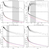 |
Fig. 1. Azimuthally averaged radial profiles of metallicity (upper panels) and surface brightness (lower panels) of the sample galaxies. Surface-brightness error bars are smaller than symbols. The surface brightness level at which sky subtraction uncertainties become dominant is μr ≥ 26 mag arcsec−2 for all the galaxies. The vertical dotted and dashed lines correspond to the transition radii Rtr, 1 and Rtr, 2, respectively, while the grey shaded areas mark the transition regions between different components of the fit. The red and magenta lines indicate the fit to the central and intermediate regions with a Sérsic profile, while the blue line indicates the fit to the outermost regions. The black line indicates the sum of the best-fitting components. The total stellar mass of each galaxy is given. |
3.2. Stellar kinematic and population properties
As we want to study the stellar kinematics and populations of the main components derived from the analysis of the surface brightness distribution, we adopted the ellipse parameters (semi-major axis, ellipticity, and position angle) of the isophotal analysis by Iodice et al. (2019b) to extract the averaged radial profiles of the stellar velocity dispersion, age, and metallicity. In this way, the photometric and spectroscopic radial profiles can be directly compared. In particular, for each sample galaxy, we assumed the semi-major-axis, ellipticity, and position-angle values derived from the isophotal fit and stacked the MUSE spaxels between two consecutive ellipses, without defining a threshold for the S/N. Since we are dealing with galaxies with a non-negligible rotation, we first rest-framed each spaxel according to the velocity maps by Iodice et al. (2019a). We then fitted the stacked spectra in order to retrieve the radial profiles of the stellar kinematic and population properties. The average S/N of the radially stacked spectra is > 80 pixel−1 and, in the worst cases, it remains higher than 40 pixel−1 along the galactocentric distance anyway, allowing us to recover reliable measurements with the template fitting technique.
The stellar line-of-sight velocity distribution (as parameterised by Gerhard 1993 and van der Marel & Franx 1993) and light-weighted age and metallicity were derived with the Penalised Pixel-Fitting code (pPXF, Cappellari & Emsellem 2004; Cappellari 2017). We adopted the α-enhanced MILES SSP with BaSTI theoretical isochrones2 and a unimodal IMF with a fixed slope of Γ = 1.3 (Vazdekis et al. 2012, 2015) as spectral templates with a resolution of FWHM = 2.51 Å (Falcón-Barroso et al. 2011). Such libraries of SSP templates are available with [α/Fe]=0.0 and 0.4 dex. We interpolated the existing α-enhanced libraries in order to create the libraries corresponding to the [α/Fe] values of 0.1, 0.2, and 0.3. We then took advantage of the mean [Mg/Fe] reported in Table 2 from Iodice et al. (2019a) in order to select the most suitable set of α-enhanced MILES among the five we have available. The stellar templates were convolved in order to match the MUSE instrumental resolution in the 4800–6400 Å fitted wavelength range. This spectral window contains age information distributed along its wavelength range (Ocvirk et al. 2006; Boecker et al. 2020). A sigma clipping routine allowed us to mask the pixels that were too noisy. In order to retrieve the stellar kinematics, we only adopted second-order additive polynomials, whereas we only used second-order multiplicative polynomials for the stellar population fit, since the order of such polynomials was high enough to retrieve minimal fit residuals. As prescribed in Shetty & Cappellari (2015), for each fit we adjusted the regularisation factor to obtain  , where
 and
and  refer to the χ2 of the unregularised and regularised solutions, respectively.
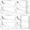 |
Fig. 1. continued. |
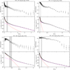 |
Fig. 1. continued. |
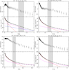 |
Fig. 1. continued. |
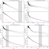 |
Fig. 1. continued. |
We thus obtained the azimuthally averaged radial profiles of stellar velocity dispersion, age, and metallicity. We further exploited the velocity and velocity-dispersion maps from the Voronoi-binned analysis performed in Iodice et al. (2019a) to retrieve, at the same aforementioned isophotal contours, the radial profiles of the specific stellar angular momentum, λR (as defined in Emsellem et al. 2011). We corrected the measured values of λR for inclination, i, using the following relation by Falcón-Barroso et al. (2019):
 (1)
(1)
where we derived i = 1 − ϵ from ellipticity, ϵ, and assumed an anisotropy parameter of δ = 0.65ϵ (Emsellem et al. 2011).
The resulting azimuthally averaged radial profiles of metallicity and r-band surface brightness for all the sample galaxies are plotted in Fig. 1, while the azimuthally averaged radial profiles of stellar velocity dispersion, inclination-corrected specific angular momentum, metallicity, and age are shown in Fig. B.1.
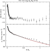 |
Fig. 1. continued. |
4. Results
In this section, we discuss how the derived stellar kinematic and population properties of the sample galaxies vary according to the transition radii between the different inner and outer galaxy components as functions of the total stellar mass and cluster environment.
4.1. Stellar kinematic and population properties as a function of stellar mass
We derived the running mean of the azimuthally averaged radial profiles of the stellar velocity dispersion, age, metallicity, and specific angular momentum of the sample galaxies in three different bins of stellar masses: 8.9 ≤ log(M*/M⊙) ≤ 10.5, 10.5 < log(M*/M⊙) ≤ 10.8, and 10.8 < log(M*/M⊙) ≤ 11.2. They are shown in Fig. 2. The choice of these stellar mass ranges is motivated by the theoretical predictions by Tacchella et al. (2019), who adopted the same mass bins to study the mass assembly history of cluster galaxies down to the lowest mass regime of ∼109 M⊙.
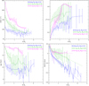 |
Fig. 2. Running mean as a function of radius of the azimuthally averaged profiles of the stellar velocity dispersion (upper left panel), inclination-corrected specific angular momentum (upper right panel), age (lower left panel), and metallicity (lower right panel) for the sample galaxies in three different mass bins: 8.9 ≤ log(M*/M⊙) ≤ 10.5 (blue symbols), 10.5 < log(M*/M⊙) ≤ 10.8 (green symbols), and 10.8 < log(M*/M⊙) ≤ 11.2 (magenta symbols). The dashed vertical lines mark the position of the average transition radius Rtr, 1 for each mass bin. The dash-dotted lines represent the fits to the metallicity gradients in the two regions defined by transition radii Rtr, 1 and Rtr, 2. The error bars trace the dispersion of the points around the mean trend. The radial profiles of the stellar kinematics and population properties of the three edge-on galaxies, FCC 153, FCC 170, and FCC 177, have been excluded from the mean. |
On average, the resulting radial profiles prove that we are able to map the stellar kinematics and population properties out to ∼1.8 Re for the more massive sample galaxies and out to ∼2.8−3 Re for the galaxies with M* ≤ 1010 M⊙. This is one of the main achievements of the F3D project, since the most extended radial profiles of the stellar kinematic and population properties, which were previously obtained with integral-field spectroscopy only, do not go beyond ∼2.5 Re (Greene et al. 2019). Recently, Dolfi et al. (2021) studied the kinematic properties of ETGs by combining the information from the stellar component obtained from ATLAS3D (Cappellari et al. 2011) and SLUGGS (Brodie et al. 2014) surveys with discrete PN and GC tracers to probe the outskirts of galaxies out to ∼4−6 Re, but only going beyond ∼2.5 Re with the discrete tracers.
As expected, according to the M* − σe relation3 (Cappellari et al. 2013) the velocity dispersion of the less massive galaxies of the sample (8.9 ≤ log(M*/M⊙) ≤ 10.5) at 1 Re ranges from 70−90 km s−1 For more massive galaxies, σe ∼ 100−120 km s−1 for 10.5 < log(M*/M⊙) ≤ 10.8 and σe ∼ 150−180 km s−1 for 10.8 < log(M*/M⊙) ≤ 11.2 (Fig. 2, upper left panel).
As already found by Iodice et al. (2019a), all the ETGs in the Fornax cluster, except for FCC 276 and FCC 213 (which is not studied here), are fast rotators with λRe ∼ 0.15−0.8. The running mean of the radial profile of λR corrected for inclination in the two less massive bins are almost flat outside Rtr, 1, while in the highest mass bin the radial profile increases beyond Rtr, 1, reaching a maximum at ∼1.5 Re and decreasing outwards (Fig. 2, upper right panel).
The stellar age radial profiles show that less massive galaxies of the sample have, on average, younger populations (aged ∼ 9−10 Gyr) than more massive galaxies (aged ∼ 11−13 Gyr). The in situ dominated regions of the galaxies (R ≤ Rtr, 1) are older than the outskirts. Such a gradient is steeper in the more massive ETGs, where the stellar population seem to be two times older inside Rtr, 1 (Fig. 2, lower left panel). Similar trends were recently found by Zibetti et al. (2020) in a sample of 69 ETGs from the CALIFA survey (Sánchez et al. 2012), which are characterised by small radial variations in the age radial profiles with an inversion of the slope at ∼0.3−0.4 Re. Moreover, they found that the higher mass ETGs are homogeneously old, while the less massive ones become increasingly younger, especially in the inner regions.
The shape of the stellar metallicity radial profile is different in the three mass bins (Fig. 2, lower right panel). For R > Rtr, 1, the metallicity radial profile is steeper for the less massive galaxies and tends to be flatter for the more massive one. This trend is confirmed by looking at the metallicity gradients4 computed in the central in situ dominated regions (i.e. for R ≤ Rtr, 1) and for R ≥ Rtr, 1, which are listed in Table 2. Similar behaviour was found for the g − i colour radial profiles of the sample ETGs obtained in the same bins of stellar masses by Spavone et al. (2020, see their Fig. 7). In detail, the colour radial profiles of the massive ETGs tends to flatten in the galaxy outskirts (i.e. beyond the transition radius from the central in-situ component).
Average metallicity gradients in the inner and outer regions of the sample galaxies.
For all galaxies of the sample, we derived the gradients of metallicity and surface brightness as Δ[M/H] = d[M/H]/dR and Δμ = dμ/dR, respectively. We found that, on average, ETGs with a higher accreted mass fraction have flatter metallicity and surface-brightness radial profiles in the outskirts (i.e. for R ≥ Rtr, 1) (Fig. 3).
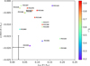 |
Fig. 3. Metallicity gradients as a function of surface-brightness gradients beyond Rtr, 1 for the sample galaxies. Data points are coloured according to the total accreted mass fraction fh, T as defined by Spavone et al. (2020). The average error bars on the metallicity and surface brightness gradients are indicated in the bottom left corner. |
4.2. Stellar kinematic and population properties as a function of the cluster environment
We derived the running mean of the azimuthally averaged radial profiles of the stellar metallicity and age for the galaxies belonging to the two main structures found in the Fornax cluster: the core-NS clump and the infalling galaxies (see Sect. 1 and Iodice et al. 2019a). They are shown in Fig. 2.
The galaxies in the core-NS clump have a milder metallicity gradient (with a slope s(R > Rtr, 1)= − 0.09 ± 0.04) in the outskirts than the infalling galaxies (s(R > Rtr, 1)= − 0.17 ± 0.05) (Fig. 4, left panel). By using the surface-brightness radial profiles and colour-based mass-to-light ratios given by Iodice et al. (2019b), we derived the stellar surface mass density for the sample galaxies. In Fig. 5, we plot the running mean of the metallicity profiles of the ETGs in the core-NS clump and of the infalling galaxies as a function of the stellar mass surface density. These profiles are compared with those obtained by Zibetti et al. (2020) for a sample of ETGs with log(M*/M⊙) < 11.3 in the CALIFA survey. As expected, due to the different prescriptions adopted for the stellar population models, an offset between the two samples is observed. Therefore, we derived the difference (∼0.05 dex) between the average metallicity value for our profiles with respect to the CALIFA ones in the 3.4 < log(μ*/M⊙ pc−2) < 4 range and shifted them using these values. The differences in the higher density inner parts are due to the different spatial resolutions of the CALIFA and MUSE observations. On average, for log(μ*/M⊙ pc) < 3.6 the trend of the metallicity profile for the infalling galaxies is consistent with that found by Zibetti et al. (2020). This similarity in shape in the outer parts is expected, given that the CALIFA survey is dominated by non-cluster galaxies. Conversely, for galaxies in the core-NS clump, the profiles start to diverge for log(μ*/M⊙ pc−2) < 2.5, where we measured a flatter profile in the outskirts of the galaxies belonging to this cluster sub-structure.
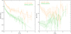 |
Fig. 4. Running mean as a function of radius of the azimuthally-averaged metallicity (left panel) and age (right panel) for the sample galaxies in the core-NS clump (orange symbols) and for those infalling in the Fornax cluster (green symbols). The dash-dotted lines represent the fits to the metallicity gradients between transition radii. The dash-dotted lines represent the fits to the metallicity gradients in the two regions defined by transition radii Rtr, 1 and Rtr, 2. The error bars trace the dispersion of the points around the mean trend. The radial profiles of the stellar kinematics and population properties of the three edge-on galaxies, FCC 153, FCC 170, and FCC 177, have been excluded from the mean. |
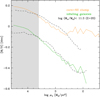 |
Fig. 5. Running mean as a function of stellar mass surface density of the average metallicity profiles for the sample galaxies in the core-NS clump (orange symbols) and for those infalling in the Fornax cluster (green symbols). The black dashed lines correspond to the CALIFA ETGs with log(M*/M⊙)< 11.3 studied by Zibetti et al. (2020). The grey shaded region marks the radial range where the difference of spatial resolution between the CALIFA and MUSE observations affect the profiles. |
The age radial profiles also appear to be quite different for the galaxies belonging the two sub-structures (Fig. 4, right panel). The galaxies in the core-NS clump are characterised by an age decreasing from ∼11 to ∼9.5 Gyr moving outwards from the centre out to about 1 Re, whereas the age remains quite constant at ∼10 Gyr at larger radii. The age radial profile of the infalling galaxies shows a dip towards the centre at R ≤ 1 Re with an age ranging from ∼7.5 to ∼8.5 Gyr and then increasing to an age of ∼ 9−10 Gyr at larger radii. Therefore, while the outskirts of galaxies in both sub-structures show comparable stellar ages, the in situ dominated regions show different behaviour, since they appear older in the galaxies belonging to the core-NS clump. The dip in the age radial profile observed towards the central regions of the infalling galaxies is due to the presence of a dynamically ‘cold’ component with a lower value of velocity dispersion (Fig. B.1).
5. Discussion and conclusions
In this work, we derived the azimuthally averaged radial profiles of the stellar velocity dispersion, inclination-corrected specific angular momentum, age, and metallicity for the brightest ETGs inside the virial radius of the Fornax cluster from the integral-field spectroscopic data of the F3D survey. To this aim, we adopted the isophotal parameters (i.e. semi-major axis, ellipticity, and position angle) of the surface photometry performed on the deep optical images obtained by the FDS survey. Therefore, the resulting radial profiles of stellar kinematic and population properties based on F3D data match the photometric radial profiles derived from FDS data.
Thanks to the extended and deep photometry, we derived the size scales of the main components dominating the light distribution of the sample galaxies. For most of them, we were able to follow the stellar kinematic and population properties well beyond the first transition radius, from the bounded in situ component to the accreted (ex situ) stellar halo. There are only a few exceptions; for FCC 310 and FCC 255 we reached only ∼0.4 Rtr, 1 and Rtr, 1, respectively, whereas for FCC 167, the F3D data extend out to the second transition radius reaching the regions of the stellar envelope (Figs. 1 and B.1).
Our combined photometric-spectroscopic analysis yielded two major results for for the brightest ETGs inside the virial radius of the Fornax cluster:
-
The galaxies in the highest (10.8 ≤ log(M*/M⊙) ≤ 11.2) and intermediate (10.5log(M*/M⊙) ≤ 10.8) mass bins have flatter metallicity radial profiles than those observed for the lowest (8.9 ≤ log(M*/M⊙) ≤ 10.5) mass bin (Fig. 2);
-
On average, the galaxies with highest accreted mass fraction (as derived from photometry) have milder gradients of both metallicity and surface-brightness radial profiles (Fig. 3);
-
It seems that a segregation in metallicity exists between the cluster members belonging to the core-NS clump and the infalling galaxies. The galaxies in the core-NS clump have a milder metallicity gradient in the outskirts (i.e. for R > Rtr, 1) than the infalling galaxies, which is not expected from the stellar mass-metallicity relation (Fig. 4).
The two main questions that we would like to address and discuss following the present work are the following:
-
How do the new results correlate with the other properties (e.g., the star formation history and accreted mass fraction) derived for the Fornax galaxies in the two sub-structures?
-
How do they fit within the general framework traced for the assembly history of the Fornax cluster?
According to Spavone et al. (2020), the massive ETGs in the sample have the highest accreted mass fraction and belong to the core-NS clump. These galaxies have flatter metallicity and surface-brightness radial profiles in their outskirts (i.e. a smaller gradient for R ≥ Rtr, Fig. 3). Conversely, the ETGs with the smaller or null accreted mass fraction are part of the infalling group of galaxies and show steeper metallicity and surface-brightness radial profiles for R ≥ Rtr.
The segregation found in metallicity and accreted mass fraction between the galaxies in the two Fornax sub-structures reinforces the idea proposed by Iodice et al. (2019a) that the core-NS clump may result from the accretion of a group of galaxies during the gradual build-up of the cluster, while the infalling galaxies entered the cluster later, no more than 8 Gyr ago. The pre-processing mechanisms in the clump induced strong gravitational interactions, which have modified the structure of galaxies in this sub-structure. This correlation is consistent with the hypothesis where the repeated mergers shaping the stellar halo around galaxies feed this component in terms of baryonic mass and produce a mixing of different stellar populations from the accreted satellites, which results in a flatter metallicity radial profile at larger radii. The lack of an extended stellar envelope in the infalling galaxies is consistent with their steeper metallicity gradients.
These results are consistent with theoretical predictions on the accretion history of ETGs based on the Illustris simulations (Cook et al. 2016; Zhu et al. 2022), where galaxies with a high accreted mass fraction display flatter metallicity gradients in their outskirts (i.e. for R ≥ 2 Re). At the same radii, a flatter surface-brightness radial profile is also found. The correlation found in simulations between the metallicity and surface brightness gradients with the accreted mass fraction is fairly consistent with the observed behaviour of our sample galaxies, as shown in Fig. 3. According to Cook et al. (2016), the relative fraction between the ex situ and in situ components determines the slope of the surface brightness and metallicity radial profiles in the galaxy outskirts, regardless of the mass assembly mechanism. Hence, the primary driver for such gradients is the total amount of the accreted mass. The stellar populations in the outskirts can equally result from major mergers or minor accretion events. The comparison of the metallicity-surface mass-density relation for the two sub-structures in the cluster with that derived for the CALIFA ETGs by Zibetti et al. (2020) further suggests that the flatter metallicity radial profile found at large radii for the NS-clump galaxies might be due to an environmental effect, since it is not expected from the stellar mass-metallicity relation (Fig. 5).
Simulations also predict that the age radial profiles tend to have a positive gradients in the galaxy outskirts. This is consistent with the age radial profiles we observed for the sample galaxies (Fig. 2, lower left panel). The absence of an evident segregation in the age radial profiles in the outskirts of galaxies between the NS clump and infalling group members (Fig. 4, right panel) is also expected from simulations, since age seems to be a poor indicator of the galaxy accretion history.
The strength and novelty of this work resides in having extended deep imaging and integral-field spectroscopy for a complete sample of galaxies in a cluster environment. To date, while there are studies showing extended stellar-kinematic and population-property radial profiles, these provide the analysis for single objects (see e.g., Dolfi et al. 2021). This work offers the chance to trace how the mass assembly varies with the stellar mass of the host galaxies and how it is connected with the environment. In addition, on a larger scale, results allow us to constrain the assembly history of the cluster where galaxies reside.
σe, is defined as the velocity dispersion contained within the half-light isophote.
The gradients are computed by fitting straight lines in log space.
Acknowledgments
We are very grateful to the anonymous referee for his/her comments and suggestions which helped to improve and clarify the paper. We wish to thank S. Zibetti for very useful discussions and suggestions. G.v.d.V. acknowledges funding from the European Research Council (ERC) under the European Union’s Horizon 2020 research and innovation programme under grant agreement No 724857 (Consolidator Grant ArcheoDyn). G.D. acknowledges support from CONICYT project BASAL ACE210002, FONDECYT REGULAR 1200495, and ANID project Basal FB-210003. K.F. acknowledges support from the European Space Agency (ESA) as an ESA Research Fellow. J.F.B. and I.M.N. acknowledge support through the RAVET project by the grant PID2019-107427GB-C32 from the Spanish Ministry of Science, Innovation and Universities (MCIU), and through the IAC project TRACES which is partially supported through the state budget and the regional budget of the Consejería de Economía, Industria, Comercio y Conocimiento of the Canary Islands Autonomous Community. E.M.C. is funded by Padua University grants DOR1935272/19, DOR2013080/20, and DOR2021 and by MIUR grant PRIN 2017 20173ML3WW-001.
References
- Barbosa, C. E., Arnaboldi, M., Coccato, L., et al. 2018, A&A, 609, A78 [NASA ADS] [CrossRef] [EDP Sciences] [Google Scholar]
- Barone, T. M., D’Eugenio, F., Colless, M., et al. 2018, ApJ, 856, 64 [Google Scholar]
- Boecker, A., Alfaro-Cuello, M., Neumayer, N., Martín-Navarro, I., & Leaman, R. 2020, ApJ, 896, 13 [NASA ADS] [CrossRef] [Google Scholar]
- Brodie, J. P., Romanowsky, A. J., Strader, J., et al. 2014, ApJ, 796, 52 [Google Scholar]
- Cantiello, M., Venhola, A., Grado, A., et al. 2020, A&A, 639, A136 [NASA ADS] [CrossRef] [EDP Sciences] [Google Scholar]
- Caon, N., Capaccioli, M., & D’Onofrio, M. 1993, MNRAS, 265, 1013 [NASA ADS] [CrossRef] [Google Scholar]
- Cappellari, M. 2017, MNRAS, 466, 798 [Google Scholar]
- Cappellari, M., & Emsellem, E. 2004, PASP, 116, 138 [Google Scholar]
- Cappellari, M., Emsellem, E., Krajnović, D., et al. 2011, MNRAS, 413, 813 [Google Scholar]
- Cappellari, M., McDermid, R. M., Alatalo, K., et al. 2013, MNRAS, 432, 1862 [NASA ADS] [CrossRef] [Google Scholar]
- Chaturvedi, A., Hilker, M., Cantiello, M., et al. 2022, A&A, 657, A93 [NASA ADS] [CrossRef] [EDP Sciences] [Google Scholar]
- Coccato, L., Gerhard, O., Arnaboldi, M., et al. 2010, Highlights Astron., 15, 68 [Google Scholar]
- Coccato, L., Gerhard, O., Arnaboldi, M., & Ventimiglia, G. 2011, A&A, 533, A138 [NASA ADS] [CrossRef] [EDP Sciences] [Google Scholar]
- Coccato, L., Arnaboldi, M., & Gerhard, O. 2013, MNRAS, 436, 1322 [Google Scholar]
- Cook, B. A., Conroy, C., Pillepich, A., Rodriguez-Gomez, V., & Hernquist, L. 2016, ApJ, 833, 158 [Google Scholar]
- Cooper, A. P., D’Souza, R., Kauffmann, G., et al. 2013, MNRAS, 434, 3348 [Google Scholar]
- Cooper, A. P., Parry, O. H., Lowing, B., Cole, S., & Frenk, C. 2015, MNRAS, 454, 3185 [Google Scholar]
- Dolfi, A., Forbes, D. A., Couch, W. J., et al. 2021, MNRAS, 504, 4923 [NASA ADS] [CrossRef] [Google Scholar]
- Drinkwater, M. J., Gregg, M. D., & Colless, M. 2001, ApJ, 548, L139 [Google Scholar]
- Emsellem, E., Cappellari, M., Krajnović, D., et al. 2011, MNRAS, 414, 888 [Google Scholar]
- Fahrion, K., Lyubenova, M., Hilker, M., et al. 2020a, A&A, 637, A26 [NASA ADS] [CrossRef] [EDP Sciences] [Google Scholar]
- Fahrion, K., Lyubenova, M., Hilker, M., et al. 2020b, A&A, 637, A27 [NASA ADS] [CrossRef] [EDP Sciences] [Google Scholar]
- Falcón-Barroso, J., Sánchez-Blázquez, P., Vazdekis, A., et al. 2011, A&A, 532, A95 [Google Scholar]
- Falcón-Barroso, J., van de Ven, G., Lyubenova, M., et al. 2019, A&A, 632, A59 [Google Scholar]
- Ferguson, H. C. 1989, AJ, 98, 367 [Google Scholar]
- Ferreras, I., Scott, N., La Barbera, F., et al. 2019, MNRAS, 489, 608 [Google Scholar]
- Forbes, D. A. 2017, MNRAS, 472, L104 [NASA ADS] [CrossRef] [Google Scholar]
- Gerhard, O. E. 1993, MNRAS, 265, 213 [Google Scholar]
- Gonzalez, A. H., Zabludoff, A. I., & Zaritsky, D. 2005, ApJ, 618, 195 [Google Scholar]
- Greene, J. E., Janish, R., Ma, C.-P., et al. 2015, ApJ, 807, 11 [Google Scholar]
- Greene, J. E., Veale, M., Ma, C.-P., et al. 2019, ApJ, 874, 66 [Google Scholar]
- Hartke, J., Arnaboldi, M., Gerhard, O., et al. 2018, A&A, 616, A123 [NASA ADS] [CrossRef] [EDP Sciences] [Google Scholar]
- Iodice, E., Capaccioli, M., Grado, A., et al. 2016, ApJ, 820, 42 [Google Scholar]
- Iodice, E., Spavone, M., Capaccioli, M., et al. 2017, ApJ, 839, 21 [Google Scholar]
- Iodice, E., Sarzi, M., Bittner, A., et al. 2019a, A&A, 627, A136 [NASA ADS] [CrossRef] [EDP Sciences] [Google Scholar]
- Iodice, E., Spavone, M., Capaccioli, M., et al. 2019b, A&A, 623, A1 [NASA ADS] [CrossRef] [EDP Sciences] [Google Scholar]
- Iodice, E., Spavone, M., Capaccioli, M., et al. 2021, The Messenger, 183, 25 [NASA ADS] [Google Scholar]
- Kluge, M., Neureiter, B., Riffeser, A., et al. 2020, ApJS, 247, 43 [Google Scholar]
- Kormendy, J., Fisher, D. B., Cornell, M. E., & Bender, R. 2009, ApJS, 182, 216 [Google Scholar]
- Kuijken, K. 2011, The Messenger, 146, 8 [NASA ADS] [Google Scholar]
- Longobardi, A., Arnaboldi, M., Gerhard, O., et al. 2013, A&A, 558, A42 [NASA ADS] [CrossRef] [EDP Sciences] [Google Scholar]
- Ma, C.-P., Greene, J. E., McConnell, N., et al. 2014, ApJ, 795, 158 [Google Scholar]
- Martín-Navarro, I., Vazdekis, A., La Barbera, F., et al. 2015, ApJ, 806, L31 [CrossRef] [Google Scholar]
- Martín-Navarro, I., Pinna, F., Coccato, L., et al. 2021, A&A, 654, A59 [NASA ADS] [CrossRef] [EDP Sciences] [Google Scholar]
- McDermid, R. M., Alatalo, K., Blitz, L., et al. 2015, MNRAS, 448, 3484 [Google Scholar]
- Napolitano, N. R., Gatto, M., Spiniello, C., et al. 2022, A&A, 657, A94 [NASA ADS] [CrossRef] [EDP Sciences] [Google Scholar]
- Ocvirk, P., Pichon, C., Lançon, A., & Thiébaut, E. 2006, MNRAS, 365, 46 [Google Scholar]
- Paolillo, M., Fabbiano, G., Peres, G., & Kim, D.-W. 2002, ApJ, 565, 883 [Google Scholar]
- Peletier, R., Iodice, E., Venhola, A., et al. 2020, ApJ, submitted [arXiv:2008.12633] [Google Scholar]
- Pillepich, A., Nelson, D., Hernquist, L., et al. 2018, MNRAS, 475, 648 [Google Scholar]
- Pinna, F., Falcón-Barroso, J., Martig, M., et al. 2019a, A&A, 625, A95 [NASA ADS] [CrossRef] [EDP Sciences] [Google Scholar]
- Pinna, F., Falcón-Barroso, J., Martig, M., et al. 2019b, A&A, 623, A19 [NASA ADS] [CrossRef] [EDP Sciences] [Google Scholar]
- Poci, A., McDermid, R. M., Lyubenova, M., et al. 2021, A&A, 647, A145 [NASA ADS] [CrossRef] [EDP Sciences] [Google Scholar]
- Pulsoni, C., Gerhard, O., Arnaboldi, M., et al. 2020, A&A, 641, A60 [EDP Sciences] [Google Scholar]
- Raj, M. A., Iodice, E., Napolitano, N. R., et al. 2019, A&A, 628, A4 [NASA ADS] [CrossRef] [EDP Sciences] [Google Scholar]
- Remus, R.-S., & Forbes, D. A. 2021, MNRAS, submitted [arXiv:2101.12216] [Google Scholar]
- Sánchez, S. F., Kennicutt, R. C., Gil de Paz, A., et al. 2012, A&A, 538, A8 [Google Scholar]
- Sarzi, M., Iodice, E., Coccato, L., et al. 2018, A&A, 616, A121 [NASA ADS] [CrossRef] [EDP Sciences] [Google Scholar]
- Scharf, C. A., Zurek, D. R., & Bureau, M. 2005, ApJ, 633, 154 [NASA ADS] [CrossRef] [Google Scholar]
- Schipani, P., Noethe, L., Arcidiacono, C., et al. 2012, J. Opt. Soc. Am. A, 29, 1359 [Google Scholar]
- Schulze, F., Remus, R.-S., Dolag, K., et al. 2020, MNRAS, 493, 3778 [Google Scholar]
- Seigar, M. S., Graham, A. W., & Jerjen, H. 2007, MNRAS, 378, 1575 [Google Scholar]
- Sérsic, J. L. 1963, Boletin de la Asociacion Argentina de Astronomia La Plata Argentina, 6, 41 [Google Scholar]
- Shetty, S., & Cappellari, M. 2015, MNRAS, 454, 1332 [NASA ADS] [CrossRef] [Google Scholar]
- Spavone, M., Capaccioli, M., Napolitano, N. R., et al. 2017, A&A, 603, A38 [NASA ADS] [CrossRef] [EDP Sciences] [Google Scholar]
- Spavone, M., Iodice, E., van de Ven, G., et al. 2020, A&A, 639, A14 [NASA ADS] [CrossRef] [EDP Sciences] [Google Scholar]
- Spavone, M., Krajnović, D., Emsellem, E., Iodice, E., & den Brok, M. 2021, A&A, 649, A161 [NASA ADS] [CrossRef] [EDP Sciences] [Google Scholar]
- Spiniello, C., Napolitano, N. R., Arnaboldi, M., et al. 2018, MNRAS, 477, 1880 [Google Scholar]
- Tacchella, S., Diemer, B., Hernquist, L., et al. 2019, MNRAS, 487, 5416 [Google Scholar]
- Trujillo, I., & Fliri, J. 2016, ApJ, 823, 123 [Google Scholar]
- van der Marel, R. P., & Franx, M. 1993, ApJ, 407, 525 [Google Scholar]
- Vazdekis, A., Ricciardelli, E., Cenarro, A. J., et al. 2012, MNRAS, 424, 157 [Google Scholar]
- Vazdekis, A., Coelho, P., Cassisi, S., et al. 2015, MNRAS, 449, 1177 [Google Scholar]
- Veale, M., Ma, C.-P., Greene, J. E., et al. 2018, MNRAS, 473, 5446 [Google Scholar]
- Venhola, A., Peletier, R., Laurikainen, E., et al. 2017, A&A, 608, A142 [NASA ADS] [CrossRef] [EDP Sciences] [Google Scholar]
- Venhola, A., Peletier, R., Laurikainen, E., et al. 2018, A&A, 620, A165 [NASA ADS] [CrossRef] [EDP Sciences] [Google Scholar]
- White, S. D. M., & Frenk, C. S. 1991, ApJ, 379, 52 [Google Scholar]
- Zabel, N., Davis, T. A., Smith, M. W. L., et al. 2019, MNRAS, 483, 2251 [Google Scholar]
- Zhu, L., Pillepich, A., van de Ven, G., et al. 2022, A&A, 660, A20 [NASA ADS] [CrossRef] [EDP Sciences] [Google Scholar]
- Zibetti, S., Gallazzi, A. R., Hirschmann, M., et al. 2020, MNRAS, 491, 3562 [Google Scholar]
Appendix A: Multi-component photometric fit of FCC 119, FCC 249, and FCC 255
This appendix provides the results of multi-component photometric fit of the FDS r-band images of FCC 119, FCC 249, and FCC 255. We obtained the azimuthally averaged surface-brightness radial profiles by following Iodice et al. (2019b) and performed the photometric fit as done by Spavone et al. (2020). The resulting observed and modelled surface-brightness radial profiles are shown in Fig. A.1, while the best-fitting structural parameters are given in Table A.1.
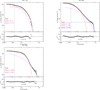 |
Fig. A.1. Deconvolved and azimuthally averaged radial profiles (open circles) from FDS r-band images of FCC 119 (upper left panels), FCC 249 (upper right panels), and FCC 255 (lower left panels). The red, magenta, and blue lines in the top panels correspond to the best-fitting first, second, and third component, respectively, while the black line shows their total surface brightness. The vertical dashed line marks the size of the galaxy core. The difference between the observed and modelled surface brightness as a function of radius is given in the bottom panels (filled circles) together with the standard deviation of the best fit (Δ, see Spavone et al. (2017) for details). |
Best-fitting r-band structural parameters for FCC 119, FCC 249, and FCC 255.
Both FCC 119 and FCC 255 are S0 galaxies. As explained in Spavone et al. (2020), for these objects the second component of the fit represents a superposition of the disc and the stellar halo. However, differently from the three S0s FCC 153, FCC 170, and FCC 177, FCC 119 and FCC 255 are low-inclined galaxies and they do not have a prominent disc. Therefore, the low-accreted mass fraction estimated for these objects can reasonably take into account a fraction of light coming from the disc component. This is consistent with the theoretical expected values for the stellar mass estimated in these galaxies.
Appendix B: Stellar kinematics and population properties of the sample galaxies
This appendix provides the azimuthally averaged radial profiles of stellar velocity dispersion, inclination-corrected specific angular momentum, metallicity, and age of the sample galaxies (Fig. B.1).
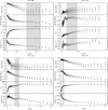 |
Fig. B.1. Azimuthally averaged radial profiles of stellar velocity dispersion, inclination-corrected specific angular momentum, metallicity, and age (from bottom to top) for the sample galaxies. The vertical dotted and dashed lines correspond to the transition radii Rtr, 1 and Rtr, 2, respectively, while the grey shaded areas mark the transition regions between different components of the fit. |
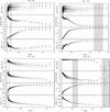 |
Fig. B.1. continued. |
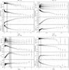 |
Fig. B.1. continued. |
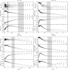 |
Fig. B.1. continued. |
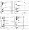 |
Fig. B.1. continued. |
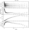 |
Fig. B.1. continued. |
All Tables
Average metallicity gradients in the inner and outer regions of the sample galaxies.
All Figures
|
Fig. 1. Azimuthally averaged radial profiles of metallicity (upper panels) and surface brightness (lower panels) of the sample galaxies. Surface-brightness error bars are smaller than symbols. The surface brightness level at which sky subtraction uncertainties become dominant is μr ≥ 26 mag arcsec−2 for all the galaxies. The vertical dotted and dashed lines correspond to the transition radii Rtr, 1 and Rtr, 2, respectively, while the grey shaded areas mark the transition regions between different components of the fit. The red and magenta lines indicate the fit to the central and intermediate regions with a Sérsic profile, while the blue line indicates the fit to the outermost regions. The black line indicates the sum of the best-fitting components. The total stellar mass of each galaxy is given. |
| In the text | |
|
Fig. 1. continued. |
| In the text | |
|
Fig. 1. continued. |
| In the text | |
|
Fig. 1. continued. |
| In the text | |
|
Fig. 1. continued. |
| In the text | |
|
Fig. 1. continued. |
| In the text | |
|
Fig. 2. Running mean as a function of radius of the azimuthally averaged profiles of the stellar velocity dispersion (upper left panel), inclination-corrected specific angular momentum (upper right panel), age (lower left panel), and metallicity (lower right panel) for the sample galaxies in three different mass bins: 8.9 ≤ log(M*/M⊙) ≤ 10.5 (blue symbols), 10.5 < log(M*/M⊙) ≤ 10.8 (green symbols), and 10.8 < log(M*/M⊙) ≤ 11.2 (magenta symbols). The dashed vertical lines mark the position of the average transition radius Rtr, 1 for each mass bin. The dash-dotted lines represent the fits to the metallicity gradients in the two regions defined by transition radii Rtr, 1 and Rtr, 2. The error bars trace the dispersion of the points around the mean trend. The radial profiles of the stellar kinematics and population properties of the three edge-on galaxies, FCC 153, FCC 170, and FCC 177, have been excluded from the mean. |
| In the text | |
|
Fig. 3. Metallicity gradients as a function of surface-brightness gradients beyond Rtr, 1 for the sample galaxies. Data points are coloured according to the total accreted mass fraction fh, T as defined by Spavone et al. (2020). The average error bars on the metallicity and surface brightness gradients are indicated in the bottom left corner. |
| In the text | |
|
Fig. 4. Running mean as a function of radius of the azimuthally-averaged metallicity (left panel) and age (right panel) for the sample galaxies in the core-NS clump (orange symbols) and for those infalling in the Fornax cluster (green symbols). The dash-dotted lines represent the fits to the metallicity gradients between transition radii. The dash-dotted lines represent the fits to the metallicity gradients in the two regions defined by transition radii Rtr, 1 and Rtr, 2. The error bars trace the dispersion of the points around the mean trend. The radial profiles of the stellar kinematics and population properties of the three edge-on galaxies, FCC 153, FCC 170, and FCC 177, have been excluded from the mean. |
| In the text | |
|
Fig. 5. Running mean as a function of stellar mass surface density of the average metallicity profiles for the sample galaxies in the core-NS clump (orange symbols) and for those infalling in the Fornax cluster (green symbols). The black dashed lines correspond to the CALIFA ETGs with log(M*/M⊙)< 11.3 studied by Zibetti et al. (2020). The grey shaded region marks the radial range where the difference of spatial resolution between the CALIFA and MUSE observations affect the profiles. |
| In the text | |
|
Fig. A.1. Deconvolved and azimuthally averaged radial profiles (open circles) from FDS r-band images of FCC 119 (upper left panels), FCC 249 (upper right panels), and FCC 255 (lower left panels). The red, magenta, and blue lines in the top panels correspond to the best-fitting first, second, and third component, respectively, while the black line shows their total surface brightness. The vertical dashed line marks the size of the galaxy core. The difference between the observed and modelled surface brightness as a function of radius is given in the bottom panels (filled circles) together with the standard deviation of the best fit (Δ, see Spavone et al. (2017) for details). |
| In the text | |
|
Fig. B.1. Azimuthally averaged radial profiles of stellar velocity dispersion, inclination-corrected specific angular momentum, metallicity, and age (from bottom to top) for the sample galaxies. The vertical dotted and dashed lines correspond to the transition radii Rtr, 1 and Rtr, 2, respectively, while the grey shaded areas mark the transition regions between different components of the fit. |
| In the text | |
|
Fig. B.1. continued. |
| In the text | |
|
Fig. B.1. continued. |
| In the text | |
|
Fig. B.1. continued. |
| In the text | |
|
Fig. B.1. continued. |
| In the text | |
|
Fig. B.1. continued. |
| In the text | |
Current usage metrics show cumulative count of Article Views (full-text article views including HTML views, PDF and ePub downloads, according to the available data) and Abstracts Views on Vision4Press platform.
Data correspond to usage on the plateform after 2015. The current usage metrics is available 48-96 hours after online publication and is updated daily on week days.
Initial download of the metrics may take a while.