| Issue |
A&A
Volume 614, June 2018
|
|
|---|---|---|
| Article Number | A72 | |
| Number of page(s) | 12 | |
| Section | Cosmology (including clusters of galaxies) | |
| DOI | https://doi.org/10.1051/0004-6361/201731445 | |
| Published online | 15 June 2018 | |
The cosmological analysis of X-ray cluster surveys
IV. Testing ASpiX with template-based cosmological simulations
1
IRFU, CEA, Université Paris-Saclay,
91191
Gif-sur-Yvette, France
e-mail: This email address is being protected from spambots. You need JavaScript enabled to view it.
2
Université Paris Diderot, AIM, Sorbonne Paris Cité, CEA, CNRS,
91191
Gif-sur-Yvette, France
3
Departments of Physics and Astronomy and Michigan Center for Theoretical Physics, University of Michigan,
Ann Arbor,
MI, USA
4
Max Planck Institut für Extraterrestrische Physik,
Giessenbachstrasse 1,
85748
Garching bei München,
Germany
5
CNRS,
IRAP, 9 Av. colonel Roche,
31028
Toulouse cedex 4, France
6
Université de Toulouse, UPS-OMP, IRAP,
Toulouse, France
7
Argelander Institut für Astronomie, Universität Bonn,
53121
Bonn, Germany
Received:
26
June
2017
Accepted:
27
January
2018
Abstract
Context. This paper is the fourth of a series evaluating the ASpiX cosmological method, based on X-ray diagrams, which are constructed from simple cluster observable quantities, namely: count rate (CR), hardness ratio (HR), core radius (rc), and redshift. Aims. Following extensive tests on analytical toy catalogues (Paper III), we present the results of a more realistic study over a 711 deg2 template-based maps derived from a cosmological simulation.
Methods. Dark matter haloes from the Aardvark simulation have been ascribed luminosities, temperatures, and core radii, using local scaling relations and assuming self-similar evolution. The predicted X-ray sky-maps were converted into XMM event lists, using a detailed instrumental simulator. The XXL pipeline runs on the resulting sky images, produces an observed cluster catalogue over which the tests have been performed. This allowed us to investigate the relative power of various combinations of the CR, HR, rc, and redshift information. Two fitting methods were used: a traditional Markov chain Monte Carlo (MCMC) approach and a simple minimisation procedure (Amoeba) whose mean uncertainties are a posteriori evaluated by means of synthetic catalogues. The results were analysed and compared to the predictions from the Fisher analysis (FA).
Results. For this particular catalogue realisation, assuming that the scaling relations are perfectly known, the CR-HR combination gives σ8 and Ωm at the 10% level, while CR-HR-rc-z improves this to ≤3%. Adding a second HR improves the results from the CR-HR1-rc combination, but to a lesser extent than when adding the redshift information. When all coefficients of the mass-temperature relation (M-T, including scatter) are also fitted, the cosmological parameters are constrained to within 5–10% and larger for the M-T coefficients (up to a factor of two for the scatter). The errors returned by the MCMC, those by Amoeba and the FA predictions are in most cases in excellent agreement and always within a factor of two. We also study the impact of the scatter of the mass-size relation (M-Rc) on the number of detected clusters: for the cluster typical sizes usually assumed, the larger the scatter, the lower the number of detected objects.
Conclusions. The present study confirms and extends the trends outlined in our previous analyses, namely the power of X-ray observable diagrams to successfully and easily fit at the same time, the cosmological parameters, cluster physics, and the survey selection, by involving all detected clusters. The accuracy levels quoted should not be considered as definitive. A number of simplifying hypotheses were made for the testing purpose, but this should affect any method in the same way. The next publication will consider in greater detail the impact of cluster shapes (selection and measurements) and of cluster physics on the final error budget by means of hydrodynamical simulations.
Key words: X-rays: galaxies: clusters / cosmological parameters / methods: statistical
© ESO 2018
1 Introduction
Clusters of galaxies constitute one of the low-redshift cosmological probes complementing early Universe measurements from the cosmic microwave background (CMB). Since cluster number counts are both sensitive to the geometry of the Universe and the growth of structure, related statistics provide, in theory, key cosmological information. But because of the many uncertainties impinging on cluster mass determination, the reliability of the cluster route has been time after time questioned. In the past few years however, there is growing evidence that independent cosmological analyses based on structure growth at low-z favour a lower σ8 than the most recent Planck CMB studies (Planck Collaboration XXIV 2016; Pacaud et al. 2016). In other words, we find fewer clusters of a given mass than the CMB cosmology predicts, given our current knowledge of cluster physics as coded in the mass-observable relations. Cluster are thus expected to provide a critical contribution to the upcoming extensive dark energy studies.
Cluster cosmology requires jointly modelling the physical parameters describing the evolution of the intra-cluster medium (ICM) alongwith the impact of selection procedure. While the first self-consistent methods have followed a backward modelling of the recovered cosmology-dependent, mass function (e.g. Vikhlinin et al. 2009), more recent studies moved to a forward approach whose likelihood includes physical quantities such as luminosity, temperature, or gas fraction (e.g. Mantz et al. 2014, 2015). Cluster number counts from Sunyaev-Z’eldovich surveys are routinely modelled in terms of the signal-to-noise ratio (S/N) or the Compton parameter of the detections, which can be related to the cluster mass via scaling relations from X-ray, lensing, or velocities (e.g. Vanderlinde et al. 2010; Hasselfield et al. 2013; Benson et al. 2013; Bocquet et al. 2015; Planck Collaboration XXIV 2016). In this context, we are developing a cosmological analysis method (ASpiX) based on X-ray cluster number counts that does not explicitly rely either on cluster mass determinations or physical quantities. This method consists in the modelling of the multidimensional distribution of a set of directly measurable X-ray clusters quantities, namely: count rates (CRs), hardness ratios (HRs), and apparent size (rc), which are all cosmology independent. This method is particularly suited to rather shallow survey-type data, when the number of collected X-ray photons is too low to enable detailed spectral and morphological analyses. Thanks to its modularity, the ASpiX method considerably eases the process by simultaneously fitting in the observed parameter space, the effect of cosmology, selection, and cluster physics. Depending on the volume surveyed, that is, the number of clusters involved in the analysis, the number of parameters that may be fitted can increase from a few to 15 or more, including in particular scatter and evolution in the scaling relations. This method cannot rival approaches including deep pointed X-ray observations along with ancillary data from other wavebands and, fundamentally, faces the same uncertainties as to the observable-mass transformation. However, the method allows the inclusion of the vast majority of the detected clusters even when only a few tens of photons are available. Furthermore, when cosmological simulations are produced at a significantly high rate, the method will allow us to totally bypass any mass estimate or scaling-relation related formalism; instead, it will solely rely on the simulations by comparing the observed and simulated parameter distributions (Pierre et al. 2017). In the end, neitherassumptions based on the hydrostatic equilibrium nor any modelling of the mass function will be necessary.
This paper is the fourth of a series aiming at an in-depth characterisation of the ASpiX method. The ultimate goal is to apply this method to the current large X-ray cluster surveys. Our philosophy is to address a few specific issues per article: Paper I (Clerc et al. 2012a) laid out the principle of the method. In Paper II (Clerc et al. 2012b), we applied ASpiX on a 347 cluster sample drawn from the XMM archive, assuming fixed scaling relations and we provided predictions for the eRosita survey. Paper III (Pierre et al. 2017) was devoted to the systematic exploration of the ASpiX behaviour by means of analytical cluster toy catalogues, including the impact of the resolution of the observed parameter space, the particular role of the cluster apparent-size information, optimisation of a fast minimisation procedure (Amoeba), error estimates, search for possible degeneracies between cosmology, and cluster physics in the various parameter-space representations. In this fourth paper, we pursue our evaluation of the ASpiX method, now in almost real-world conditions, i.e. by analysing synthetic X-ray images. We assume a more realistic error model for the observable quantities, we study the effect of using a second hardness ratio (HR) and of scatter in the mass-size relation, we detect the impact of projection effects in the selection function, and we compare the Amoeba-dependent minimisation and error estimates with a standard MCMC fitting. The next, and last, validation article will quantitatively evaluate the systematic errors by means of hydrodynamical simulations.
The synthetic images in the present paper are produced by applying emission template forms to halo populations realised in N-body simulations. The images are transformed into XMM observations taking into account all instrumental and background effects. The simulated images are in turn processed as regular XMM pointings and the detected clusters of galaxies are selected following a well-defined procedure. Finally, the ASpiX method is run on the selected sample and the derived cosmological parameters are compared to those of the input numerical simulations.
The paper is organised as follows. The next section recalls the basis of the ASpiX method. Sect. 3 describes the numerical simulations and mapping of the X-ray properties onto the dark matter haloes. Sect. 4 explains the transformation of the simulated X-ray sky maps into XMM images. The reduction of the XMM images along with the production of the resulting cluster catalogues is presented in Sect. 5. The results of the cosmological analysis of the cluster catalogues are given in Sect. 6. In Sect. 7, we analyse the results and impact of particular cluster parameters. The last section draws conclusions and outlines future steps. The cosmological model adopted for this test-case study is presented in Sect. 3.1 and summarised in Table 1.
Main cosmological and cluster physics parameters used in this study.
2 The ASpiX method
In what follows, we assume that the X-ray observations are performed with an XMM survey, but the principle can be easily translated to any X-ray telescope (e.g. Chandra or eRosita).
2.1 Modelling the cluster population in the XOD
The principle of the ASpiX method consists in the fitting of a multidimensional distribution of X-ray observable parameters drawn from a selected cluster population. The so-called X-ray observable diagrams (XOD) involve part or all of the following parameters: instrumental CRs and HRs in well-specified bands, a measurement of the cluster angular size (rc) and the redshift (z, assumed to be measured by optical ground-based observations). The method relies on the fact that the cluster mass information as a function of redshift, that is our link to cosmology, is encoded in the combination of these parameters. In practice, we model XODs after assuming:
-
a cosmological model;
-
a clustermass function;
-
X-ray cluster scaling relations, including scatter and evolution (M–T, L–T, M–Rc);
-
a plasma code to transform luminosities into fluxes as a function of temperature, abundances, and redshift;
-
a model for the X-ray cluster emission profile;
-
the XMM response to convert fluxes into CRs and a PSF model to convolve the cluster profiles;
-
total area and XMM exposure time for the survey in question;
-
an error measurement model and a realistic cluster selection function for a given detection pipeline, calibrated using extensive simulations.
The numerical ingredients of the model are given in Sect. 3. We stress that, because clusters are extended sources, the cluster selection is performed in a two-dimensional parameter space, [CR, rc], which is equivalent to the physical (flux, apparent size) plane. The adopted selection function is analogous to that of the XXL survey (Pierre et al. 2016) and is given in Fig. 1; Paper III provides a detailed description. An example of a four-dimensional XOD is shown in Fig. 2.
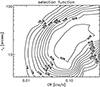 |
Fig. 1 Selection function adopted for the present study. The probability to detect a cluster as C1 is given by the isocontours as a function of CR and rc. This map was derived from extensive XMM image simulations and the two axes stand for the true (input) cluster parameters; it is thus only valid for the conditions under which the simulations were run (XMM exposure time of 10 ks and background). |
 |
Fig. 2 X-ray observable diagram computed for a 700 deg2 cluster survey, observed with 10 ks XMM exposures. Panels 1-6: 2D projections of the distribution of the four cluster parameters involved in the present study: CR in [0.5–2] keV, HR1 ([1–2]/[0.5–1] keV), HR2 ([2–5]/[0.5–2]) keV, angular cluster size rc. The diagrams are integrated over the 0 < z < 2 range, but this fifth dimension can be uncompressed if redshifts are available, which significantly increases the cosmological constraining power of the ASpiX method. Error measurements are not implemented in this example. |
2.2 Fitting the X-ray observable diagrams
The cosmological analysis of an X-ray cluster survey with ASpiX consists in finding the combination of the cosmological and cluster physics parameters that best fits the observed XOD. This is carried out by varying the parameter values of the model. The number of parameters that can be simultaneously fitted depends on the survey area and measurement accuracy. An obvious choice for the minimisation procedure is the MCMC approach and this method was adopted for the fitting of the XOD obtained from the XMM archive in Paper II. The computer time, however, increases very rapidly as a function of the number of free parameters when four-dimensional XOD are considered and hence becomes prohibitive for the current testing phase. We thus favour a simple minimisation procedure (Amoeba, Nelder & Mead 1965), which allows us to identify the most likely solution in a relatively short time. The drawback is that this procedure does not provide uncertainties on the best fitting parameters. However, as shown in Paper III, reliable error estimates can be obtained by averaging the output from at least ten different toy-catalogue realisations, drawn for that purpose. In this paper, we run both approaches in parallel to test the consistency of the results. As a complement, we give the predictions from the Fisher analysis (FA). Although, strictly speaking, only valid for Gaussian posterior distributions, this analysis provides us with a potentially quick tool to perform cosmological predictions; it is thus useful to estimate how close these predictions are to the results that we ought to achieve.
2.3 General settings of the present study
Keeping in mind the goal of the present paper, that is testing ASpiX on synthetic surveys from cosmological simulations, we use the following:
-
the Aardvark simulations (Sect. 3.1), which provide us with a projected light cone of dark matter haloes over a volume of some 700 deg2 out to a redshift of 2;
-
the cluster physics parameters listed in Sect. 3.3 with two options for the cluster emissivity profiles to map the X-ray properties of dark haloes (Table 2);
-
XMM individual observing times of 10 ks;
-
the detection pipeline and the C1 cluster selection function that are routinely used for the XXL survey;
-
either the simple Amoeba minimisation procedure or a MCMC analysis.
In the framework of testing the ASpiX method in increasingly realistic conditions, the most significant upgrade with respect to Paper III is the fact that cluster detection is now performed on maps having a more realistic distribution of source haloes than the toy catalogues. We also take the opportunity to investigate the effect of cluster core radii and of scatter in the M-Rc relation on the number of detected clusters, hence on the cosmology. We consider a more realistic model for the measurement errors. Moreover, we introduce a second HR, HR2 = [2–5]/[0.5–2] keV in addition to HR1 = [1–2]/[0.5–1] keV.
We describe in the next three sections the production of simulated XMM cluster catalogues, which constitute the input of our cosmological analysis.
Adopted values for the X-ray emission profile of the Aardvark simulated haloes.
3 Large-scale X-ray emissivity maps of the intra-cluster medium
We present in this section the production of 25 deg2 emissivity maps of the ICM using template-based N-body simulations.
3.1 Aardvark simulations
We employed N-body simulations produced on XSEDE resources (Erickson et al. 2013) with a lightweight version of the Gadget code developed for the Millennium Simulation (Springel 2005). Three simulations, of 1.05, 2.6, and 4.0 Gpc3 h−1 volumes, were used to produce a sky survey realisation covering 10 000 deg2 that resolves all haloes above 1013.2 M⊙ within z ≤ 2. The resulting sky catalogue is built by concatenating continuous light-cone output segments from the three different N-body volumes using the method described in (Evrard et al. 2002). The smallest volume maps z < 0.35, the intermediate maps 0.35 ≤ z < 1.1, and the largest volume covers 1.1 ≤ z < 2. The simulations employ 20483 particles, except for the 1.0 Gpc3 h−1 volume, which uses 14003, and corresponding particle masses are 0.27, 1.3, and 4.8 × 10¹¹ M⊙ h−1. The Aardvark suite assumes a ΛCDM cosmology with cosmological parameters Ωm = 0.23, ΩΛ = 0.77, Ωb =0.047, σ8 = 0.83, h = 0.73, and ns = 1.0. The Rockstar algorithm is used for halo finding (Behroozi et al. 2013). We refer to this suite of runs as the Aardvark simulation (for more detail see Farahi et al. 2016). Figure 3 compares the mass function of the Aardvark haloes to the Tinker haloes (Tinker et al. 2008), which is used in our analytical fit model.
3.2 X-ray properties of clusters with template approach
Starting from the Aardvark dark matter halo population, we mapped the ICM properties using a standard population model (Evrard et al. 2014). These models are motivated by theoretical arguments (Kaiser 1986) and they rely on empirical data reflecting our current knowledge of the baryonic component, which mostly pertains to the high end of the mass function. We extrapolated these models to lower mass haloes to include galaxy groups, which constitute the bulk of the population encompassed by our selection function (Fig. 3). We followed the traditional modelling of the cluster gas mass and X-ray properties by means of power-law scaling relations and assume log-normal covariance. These assumptions are supported by numerous observations, theoretical arguments, and simulation findings (e.g. Kaiser 1986; Kravtsov et al. 2006; Le Brun et al. 2014; Mantz et al. 2016; McCarthy et al. 2017).
Practically, we began with the mass, redshift, and sky location of dark matter haloes in the Aardvark simulation. Then, we used scaling relations to infer the mean gas temperature and bolometric luminosity. By means of the APEC plasma code, we deduced the X-ray fluxes in the bands of interest for the present study, namely: [0.5–1.0], [1.0–2.0], [0.5–2.0], and [0.2–5.0] keV. The halo X-ray surface brightness profiles were assumed to follow a β model. This allowed us to produce theoretical X-ray emissivity maps, of which we show an example in Fig. 5. At this stage, we stress that only the [0.5–2] keV map is used in the current study: this is the band where the source detection is performed; fluxes in the other bands are analytically derived (Sect. 5.1).
 |
Fig. 3 Cumulative dark matter halo number density as a function of mass at different epochs. Blue dots show Aardvark simulations. The pink areas show the mass range encompassed by the C1 selection. The mass scale of 1013.2 M⊙ represents the halo mass resolution limit of the simulations. |
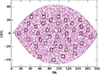 |
Fig. 4 Sky maps of the 39 regions extracted from the Aardvark simulations. Each square covers 25 deg2. Magenta dots show all haloes with a mass larger than 1014 M⊙. The simulation depth is 0 < z < 2. |
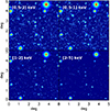 |
Fig. 5 Typical ICM emissivity maps from the Aardvark simulations. The panels show a 25 deg2 field in the fourbands of interest for the current study, namely: [0.5–2] keV, [0.5–1] keV, [1–2] keV, and [2–5] keV. No background, instrumental effects, or AGN are added. Cluster detection is performed in the [0.5–2] keV band. |
3.3 Ingredients of the cluster modelling
The particular ingredients of the cluster X-ray mapping are given in the following paragraphs.
3.3.1 Mass overdensity
The Tinker mass function is computed at an overdensity of δρ = 200 (mean density) and transformed into a function of M200c (critical) by means of a NFW profile and a concentration-mass relation (Navarro et al. 1997; Hu & Kravtsov 2003; Bullock et al. 2001). To switch from the M200c parameter of the Aardvark simulations (and the M200c Tinker mass function) to the M500c value, we assume the empirical relation M500c∕M200c = 0.714, following Lin et al. (2003). This is used for the scaling relation of Rc (see below).
3.3.2 X-ray luminosity and temperature
We model the cluster scaling relations as power laws following self-similar evolution:
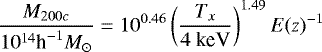 (1)
(1)
(Arnaud et al. 2005).
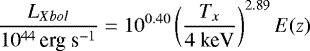 (2)
(2)
In both relations, we allow for intrinsic scatter σlnT|M and σlnL|T. Scatter in both measures, which reflects the various merging histories and relaxation states of the haloes, are assumed to be uncorrelated and independent of redshift and mass. We take 0.1 and 0.27 for σlnT|M and σlnL|T, respectively.
3.3.3 Cluster profiles
Haloes are assumed to be spherically symmetric:  . Cluster surface brightness profiles are modelled with a simple standard β profile (Cavaliere & Fusco-Femiano 1976),
![Mathematical equation: \begin{equation*} S(r) = S_0 \Bigg [ 1+\Bigg ( \displaystyle \frac{r}{r_{c}}\Bigg)^2 \Bigg]^{-3\beta +1/2},\end{equation*}](/articles/aa/full_html/2018/06/aa31445-17/aa31445-17-eq4.png) (3)
(3)
where r and rc are the projected profile coordinate and the rc. The cluster angular size (rc) is given by rc[arcsec] ∝ Rc[Mpc]∕Da(z)[Mpc], where Da is the angular distance diameter. We further relate the cluster rc to the cluster size by Rc = xc × R500, which yields
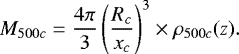 (4)
(4)
We analysed the OWLS hydrodynamical simulations (Le Brun et al. 2014) to obtain a plausible mean estimate, given the redshift and mass ranges pertaining to the present study. Assuming a β of 2/3, we find a mean value of 0.24 (a value also observationally found in Paper II) for xc with a  of 0.5. In the present paper, we stuck to a constant 0.24 value, allowing or not for scatter. We thus analysed two X-ray mappings of the Aardvark haloes as summarised in Table 2. In the final discussion, we explore the impact of other xc and scatter values on the number of detected clusters. The cluster physics parameters assumed for this study are summarised in Table 1.
3.4 Photon maps
We extracted from the Aardvark simulated sky 39 subregions of 25 deg2 each, randomly distributed and sufficiently distant from each other, such that the effects of covariance between the samples are negligible when considering the total area of 975 deg2 (Fig. 4). The size of the individual regions was chosen such as to match that of the two XXL fields. The large number of subregions provides us with a useful handle to estimate the uncertainty on the cosmological parameters via ASpIX in its Amoeba implementation.
The bolometric luminosity, temperature, and X-ray profile are ascribed to each halo characterised by its mass and redshift, following the prescriptions of Sect. 3.3. From this, we map the X-ray halo emissivity in our detection band ([0.5–2] keV) by means of the APEC X-ray plasma code (Clerc et al. 2012a; Pierre et al. 2017)following the atomic densities reported by (Grevesse & Sauval 1998); we take a mean metallicity of 0.3 Z⊙ and a mean galactic absorption corresponding to NH = 3 × 1020 cm−2. This step provides us with ICM emissivity maps; a further example is presented in Fig. 7.
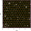 |
Fig. 6 Layout of the XMM pointings over a single 25 deg2 region; the observations are separated by 10′ in RA and Dec. Source detection is performed out to a radius of 13′ (red circles). For the cosmological analysis only sources in the innermost 10′ are considered (green circles). To avoid border effects, we discarded all detections outside the magenta square. |
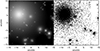 |
Fig. 7 Left: example of an ICM X-ray emissivity map in the [0.5–2] keV band. Right: corresponding photon image assuming a 10 ks exposure and a collecting area of 1000 cm2. The images are 30′× 30′ and have a pixel size of 2.5′′. |
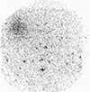 |
Fig. 8 Simulated XMM image (MOS1+MOS2+PN, 2.5′′ pixel) obtained for a 10 ks exposure on the region shown in Fig. 7. The AGN population and diffuse background components are added to the ICM emission modelled from the Aardvark simulation. All instrumental effects such as the detector spectral responses, the vignetting function, and the PSF are taken into account. |
4 XMM synthetic surveys
We describe in this section the conversion of the ICM emissivity maps into XMM images.
4.1 Survey geometry
The tiling ofa single 25 deg2 field by XMM observations is shown in Fig. 6. The XMM field of view is 15′ but given that the point spread function and the sensitivity are rather poor at large off-axis, we restricted the source detection to an off-axis of 13′ and considered only the innermost 10′ for the cosmological cluster sample. Moreover, to exclude border effects, we trimmed all 5 × 5 deg2 fields off by 5′. This yields a cosmological area of 18.22deg2 for each subregion, i.e. a total of 710.6 deg2. The number of XMM observations processed in one band reaches ~ 9000. The observations are assumed to be performed with 10 ks exposures and the THIN filter.
4.2 Conversion into XMM images
The Aardvark [0.5–2] keV band maps produced in Sect. 3.4 are 2.5′′ images in unit of photons/s/cm2. To convolve with the XMM spectral response and effective area, we assumed a mean photon energy of 1 keV for all photons, and pixel physical fluxes are transformed into XMM CR unit. The PSF distortions as well as the vignetting are then applied. This is carried out separately for the three XMM detectors, each with its own specific energy and spatial response to yield, in the end, event lists as for real observations.
4.3 Back- and foreground photons
In order to produce most realistic XMM images, the event lists obtained from the ICM are merged with those coming from other source of emission, namely: foreground and background AGN and the various components of the diffuse X-ray background. This latter contribution is summarised in Table 3. The adopted mean particle background is an average of XMM observations obtained with the closed filter. The diffuse and soft proton backgrounds follow the model proposed by (Snowden et al. 2008). The X-ray AGN population is taken from the log N – log S by Moretti et al. (2003) down to a flux limit of 10−16 erg cm−2 s−1. The AGN are randomly distributed over the XMM field of view, ignoring in the present paper, their spatial correlation and the fact that AGN may be present in cluster centres. The AGN point-like sources are convolved with the same instrumental effects (energy response, PSF, and vignetting) as for the ICM diffuse emission. Figure 8 shows an example of a final simulated XMM image.
Background components added to the ICM event list for the [0.5–2] keV band, in which the cluster detection is performed.
5 Creation of the C1 cluster cosmological catalogues
The synthetic observations are processed with the XAMIN pipeline in the same way as real standard XXL observations (e.g. Pacaud et al. 2006; Pierre et al. 2016). We extracted the C1 cluster candidates from the pipeline output lists. More than 4500 clusters were detected for realisations B0 and B0.5.
5.1 Correlation with the input catalogues
For real observations, the XAMIN pipeline is used only at the cluster detection stage on the individual XMM observations. First, source detection is routinely perform within the innermost 13′ of the detector but we usually restrict the cosmological sample to the inner 10′, which is the radius at which the sensitivity reaches 50% of the on-axis value (Clerc et al. 2012a). Second, measurements of cluster properties are subsequently performed in a semi-interactive mode (e.g. Giles et al. 2016) to cope in an optimal way with the particularity of each source, for example AGN contamination, local background removal, and possible irregular cluster shapes. This is an important step since the quality of the cosmological analysis heavily relies on the precision of these measurements.
For the present test-study based on simulations, it was not conceivable to measure some 2 × 4500 objects in this way. We thus correlated the pipeline output catalogues with the input simulated catalogues containing the cluster mass, luminosity, temperature, and rc information.In this way, we were able to assign to each detected C1, total XMM CRs in the chosen bands, following the same principles asdescribed for the production of the [0.5–2] keV CR map. As in previous studies (Pacaud et al. 2006), we used a 37.5′′ radius for the correlation with the Aardvark cluster list and a 6′′ radius for the random AGN list. The correlation outputs were flagged as follows:
-
cluster: when a C1 source is matched to an input Aardvark halo;
-
AGN: when C1 source is matched to an input AGN (rare case);
-
ambiguous: when the two previous conditions are both true;
-
false: when none of the previous conditions are true.
The results of the correlation are reported in Table 4. These results show a somewhat higher C1 contamination rate than reported in our previous analytical simulations (Pacaud et al. 2006). The ~ 5% fraction of fake sources can be explained by the fact the analytical simulations avoided cluster overlap, while projection effects naturally occur when using a cosmological light cone, creating multiple cluster detections for some peculiar lines of sight. In the real observation regime, the C1 catalogue is systematically screened by two independent persons to remove obvious fake detections.
C1 sources correlated with the input Aardvark halo and AGN catalogues.
5.2 Cosmological sample
By restricting the cluster catalogue to the inner 10′ we expected a higher S/N for the detected sources and a better positional accuracy. We excluded from the cosmological sample all sources flagged as AGN and fake. We subsequently define the C1 CLEAN sample as the C1 sources flagged as cluster and ambiguous within 10′ and consider this subsample as the best trade-off between a fully automated procedure and a dedicated interactive screening. The corresponding CLEAN survey area amounts to 710.56 deg2 with XMM. The C1 density is 6.3 deg−2 is 6.1 deg−2 for the B0 and B0.5 configurations, respectively.
5.3 Measurement errors
The last step is to ascribe realistic error measurements to each cluster parameter entering the XOD. The chosen error model is presented in Fig. 9 and is based on our experience with analytical simulations. This error model is applied to the total CRs and to the rc derived from the Aardvark catalogues (Sect. 5.1). To simplify the formalism, errors are given as a function of the [CR, rc] combination(which is also the plane used for the cluster selection) and we assume that they have the same amplitude for CR, HR1, and rc; for the second colour, HR2, we double this value given the XMM sensitivity drop in the hard band. The effect of the error measurements on the XODs is illustrated in Fig. 10.
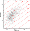 |
Fig. 9 Red lines show the adopted measurement error model as a function of the nominal total [0.5–2] keV CR and apparent rc; the black circles are the detected Aardvark C1 clusters, drawn to highlight the cluster locus in this parameter space. Practically, the error on CR and rc are randomly ascribed from a log-normal distribution with the dispersion given by the red abacuses. Errors on HR1 and HR2 are assumed to be respectively the same and the double values obtained for the corresponding [CR, rc] combination. The model assumes a mean vignetting value. |
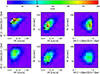 |
Fig. 10 Effects of measurement errors on the C1 CLEAN sample. The plots show from left to right the 2D diagrams CR-HR, CR-rc, and HR-rc. The first rowstands for the nominal CR, HR, and rc values stored in the Aardvark catalogues. The second row shows the result of the implementation of the error model displayed in Fig. 9. |
6 Cosmological fit
We now describe the cosmological fit on the Aardvark catalogue of X-ray haloes, prepared as described in the previous sections. Our basic analysis sticks to the same set of free parameters as in Paper III, namely [Ωm, σ8, xc, w0], assuming that the scaling relations are known and evolve self-similarly. In a second step, we open as free parameters, the coefficients of the M-T relation. The Amoeba cosmological fitting on the XOD is extensively described in Paper III and is summarised Sect. 2.2. For the MCMC analysis on the same XOD, we use a Metropolis-Hastings algorithm (Metropolis et al. 1953). Parallel chains are considered to have converged by applying the Gelman-Rubin criterion with r < 1.03 (Gelman & Rubin 1992). The fit results are discussed in Sect. 7.
6.1 Analysis of 700 deg2 survey
6.1.1 Testing constraints from mass distribution alone
Figure 3 shows an overall excellent agreement between the measured Aardvark mass function and the Tinker modelling assumed in our XOD fit. A moderate deviation is nevertheless observed in the high-redshift slice above log (M) ~ 14.5 M⊙, which is a range expected to have a high weight in the cosmological analysis. In order to test the impact of this particular uncertainty, we thus first run the cosmological fit on the mass function alone. We assume, first, an ad hoc pure mass selection giving 4296 clusters, which is very comparable to the number of C1 clusters (Table 4); and, second, no error measurements on the masses (in the selection and cosmological analysis).
The selection is shown in Fig. 11 and the results, along with the FA predictions, are given in Table 5. The cosmological fit for this particular halo catalogue was performed with Amoeba on the [M500, z] distribution using 100 different starting points, as for the XODs. We mention at this stage that the xc value is poorly constrained since this parameter does not intervene in any stage of the mass fit, the selection, nor in the mass measurements, which are assumed to be perfect. The conclusion of this exercise is that the 5% discrepancy observed at the high end of the mass function, between the fitting model and simulations, has a negligible effect on the cosmological analysis given the size of the assumed measurement uncertainties.
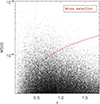 |
Fig. 11 X-ray analogous mass selection used to test the impact of the deviation between the Aardvark and Tinker mass functions. |
6.1.2 Signal variable diagrams
We now turn to the cosmological analysis of the C1 “CLEAN” Aardvark catalogue and test combinations involving an increasing number of signal variables, i.e. CR-HR1, CR-HR1-rc, z-CR-HR1-rc, CR-HR1-HR2-rc. All diagrams include scatter in the scaling relations (L, T, Rc) and error measurements as described above. Each XOD diagram is fitted using, either a MCMC method (providing uncertainties) or 100 Amoeba runs. Given that the Amoeba route does not provide errors on the output parameters, we estimate them by averaging the results of 10 × 700 deg2 analytical toy catalogues, following the methodology introduced in Paper III. We also provide the predictions from the FA. The results are gathered in Table 6. The graphic representation of the MCMC output is shown in Figs. 12 and 13.
Summary table for the cosmological analysis of the Aardvark C1 CLEAN catalogue over 711 deg2.
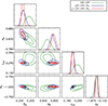 |
Fig. 12 Confidence regions at the 68% and 95% levels and 1D marginalised distribution for the studied parameter subset (Ωm, σ8, xc, w0). The cross indicates the fiducial model. The MCMC analysis was run on an effective sky area of 711 deg2 for the CLEAN C1 catalogue, involving some 4300 clusters. Fit for z−CR-HR-rc is shown in red, for CR-HR-rc is shown in blue, and for CR-HR in green. |
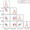 |
Fig. 13 Same as Fig. 12, for other observable combinations. This figure enables a visual comparison of the relative constraining power of z and HR2. |
6.1.3 Scaling relation evolution
We also investigated the behaviour of ASpiX in the case where the parameters of the M-T relation are totally unconstrained. In this configuration we switch from four to nine free parameters. The results are reported in Table 7.
Fit results (CR-HR-rc-z) over the 711 deg2 Aardvark C1 CLEAN catalogue when cosmological and cluster physics parameters are let free.
6.2 Analysis for the 39 × 18.22 deg2 surveys
In a secondstep, we investigated the constraining power of the 18.22 deg2 individual maps. This is of particular practical interest since these represent approximately the coverage of one XXL survey field, when considering the innermost 10′ of the XMM detector. In Fig. 14, we compare the redshift distribution of the 39 Aardvark subfields with that of XXL. While the many parameters of our Aardvark modelling ought not to be totally matching reality as viewed by both XXL fields (cosmology, scaling relations, and XMM background), the overall shapes of the redshift distributions appear to be very compatible.
We tested the CR-HR1-rc-z and CR-HR1-HR2-rc XOD by applying the Amoeba fitting on our set of free parameters. The results presented in Table 8 summarise the 3900 fits (100 for each catalogue); errors are approximated by the 1σ deviation from the mean of the 39 averaged best-10 fits obtained from each sub-catalogue. For comparison we show the predictions from the FA.
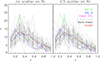 |
Fig. 14 Redshift distribution of the detected C1 Aardvark clusters for the for B0 (left) and B0.5 (right) profile configurations. Grey lines show the cluster selected population and correspond each to 18.22 deg2 map. The black dash-dotted line stands for the mean and the error bars show the 1σ deviation. The red dashed line shows our fiducial model (X-ray mapping of the haloes + analytical selection). All distributions are normalised to 13.8 deg2 to match the effective area of the XXL northern (green solid) and XXL southern (blue solid) fields considering only the pointing innermost 10′ (XXL PaperXX, Adami et al. 2018). The mean of the two XXL fields is in magenta. |
Cosmological analysis performed on the Aardvark C1 CLEAN samples corresponding to the 39 × 18.22 deg2 sub-maps (effective area).
7 Discussion
The purpose of the present article is to quantify the behaviour of the ASpiX method in more realistic conditions than the preliminary study presented in Paper III, based on analytical toy catalogues. Here, the use of template-based simulations, transformed into real-sky XMM images, allowed us to implement the effect of the selection function as well as a more realistic error model for the considered variables. We globally confirm the very positive results of Paper III and discuss our findings below.
7.1 Error estimates on cosmological parameters - 711 deg2 catalogue
Table 6 summarises the main outcome of the study, where we compare for the 711 deg2 survey (i) the effect of adding signal variables, (ii) the errors returned by the MCMC and Amoeba fitting methods, and (iii) the prediction of the FA. At this stage, we assume that the cluster scaling relations are perfectly known.
Logically, considering successively CR-HR, CR-HR-rc, and CR-HR-rc-z, the uncertainties decrease when the number of dimensions describing the cluster population increases. We recall here that the errors from the Amoeba fitting are quantified by running numerous (≥ 10) independent realisations of simulated catalogues. Given that only one 711 deg2 realisation was available, we analytically created ten 700 deg2 toy catalogues. The differences with respect to the 711 deg2 simulation is that the objects were created following the Tinker mass function exactly and were not selected in situ by the XAMIN pipeline; they were instead selected using the analytical selection function (Fig. 1), which is the same that is used for fitting the XOD and performing the FA. But the error model on the observables is the same.
All numbers recorded in Table 6 are shown with three decimal digits for the purpose of comparison, but this should not be ascribed a high significance, since not all systematic effects have been considered in the error budget. All in all, the three approaches deliver very comparable error estimates, somewhat larger for Amoeba, hence better bracketing the fiducial cosmological model. Interestingly, the fit of the N(M, z) distribution, assuming no error on mass and a perfect selection function (Table 5) does not appear to produce better results than CR-HR-rc-z in real-sky conditions for w0; the FA predictions are indeed at the same level. Table 6 suggests that, with our current working hypotheses, any deviation between the Aardvark mass function with respect to the Tinker mass function has a negligible impact on our results.
Finally, we compared the efficiency of adding a forth dimension to the XOD: either as redshift (run A3) or as a second X-ray colour (HR2, run A4). Although both induce a significant improvement with respect to CR-HR1-rc, the redshift information appears to outperform the colour information (as inferred from the error bars). This is easily understandable since only the knowledge of redshift breaks the temperature-redshift degeneracy in a pure Bremsstrahlung spectrum. The addition of a second colour solely brings a second measurement (hence refining the first measurement) of the T∕(1 + z) degeneracy (cf. bottom central panel of Fig. 2). Of course, the spectra considered in this work contain emission lines from metals (APEC plasma code), but given the small number of collected photons, the effect on thedegeneracy is small.
We note that the particular Aardwark realisation seems to converge (when z is available) to a point that is beyond the 1σ error for σ8 and Ωm, but perfect for w0 and xc; this is not unexpected from the statistical point of view. Indeed, among the 10 × 700 deg2 toy models generated for this study, we also found two catalogues yielding somewhat displaced values of Ωm = 0.223, σ8 = 0.842, xc = 0.240, w0 = −1.036.
7.2 Error estimates on the cosmological parameters - 39 × 18 deg2 catalogues
Another way to scrutinise the ASpiX output is to apply the method individually on the 39 × 18.22 deg2 subregions whose assembly constitutes the 711 deg2 area. By averaging the Amoeba fitting of each XOD, we obtain the mean uncertainty on the cosmological parameters expected for a 18.22 deg2 area. The results are given in Table 8. The mean values are well within the 1σ expectations. These error estimates are comparable to the Fisher predictions, but do not exactly follow the expected SQRT(area) scaling as can be inferred from Table 6. It is likely that with such a small area (some 110 clusters in average per field) the sampling of the XOD in its four dimensions has to be revisited to optimise the fitting procedure. We defer this question to a future paper.
7.3 Fitting cosmology along with cluster scaling relations
In Paper III, we showed that for large enough surveys it is possible to fit at the same time, and to recover with excellent accuracy, the cosmological parameters and coefficients of both cluster scaling relations (scatters were assumed to be known). This was demonstrated assuming a 10 000 deg2 area and using the Amoeba fitting. Here, we show in Table 7 the results of the MCMC fit for the 711 deg2 Aardvark catalogue when the coefficients of the M-T relations are let free, as well as the scatters of the M-Rc and M-T relations. While the cosmological parameters, the M-Rc relation and the slope of the M-T relation can be recovered at a level better than 10%, we observe larger errors for the amplitude, evolution, and scatter of M-T. This is not surprising as the scatter has a strong effect on the cluster selection selection process, hence induces additional degeneracy in the cosmological analysis (Pacaud et al. 2006; Allen et al. 2011). In this run, the coefficients of the L-T relation are held fixed. In practice, the L-T relation is the easiest cluster scaling relation to determine and can be easily computed for a 10 ks cluster sample (e.g. Giles et al. 2016); it can then be plugged as a prior into the cosmological analysis (e.g. Pacaud et al. 2016).
On average, the MCMC errors are smaller than predicted by the FA (and do not always bracket the input fiducial values). We explain this by the fact that, so far, we do not allow for uncertainties in the selection function. When both cluster physics and cosmological parameters are let free, the MCMC may converge to a peculiar solution (close to the fiducial solution, but with a higher likelihood); the MCMC may ascribe errors that are too small to its preferred solution because it is forced to consider the cluster catalogue as perfect.
Finally, we investigated in more detail the effect of the scatter in the M-Rc relation on the number of detected clusters. Table 9 summarises our calculations, still assuming the C1 selection function. The results indicate that the detection rate depends in a non-intuitive manner on the cluster size and scatter: for 0.1 < xc < 0.24, the more peaked the clusters and the smaller the dispersion, the larger the number of detected clusters; for xc = 0.4, the smaller the dispersion, the smaller the detection number. Hence, for the range of xc values usually postulated (xc = 0.1–0.24), the scatter of the M-Rc relation has the opposite effect as that of the L-T relation.
C1 cluster density (analytical calculations) as a function of cluster intrinsic size (Rc) and scatter inthe M − Rc relation.
8 Summary and conclusions
This article presents an in-depth formal analysis of ASpiX, an observable-based method for the cosmological analysis of X-ray cluster surveys. The basic working hypothesis is that only shallow survey data are available, which enable the measurements of cluster count rates, hardness ratios, and apparent sizes. The method allows the inclusion of all detected clusters and combines in a single fitting procedure the cosmological parameters, cluster scaling relations, and survey selection function. The tests are performed on a 711 deg2 semi-analytical simulation (Aardvark). The perfect X-ray emissivity sky map associated with the dark matter haloes is in turn converted into XMM event lists, using a state-of-the-art procedure that reproduces all observational effects. Clusters of galaxies are then detected and selectedusing the XAMIN XXL pipeline.
The main upgrades with respect to Paper III, based on analytical toy catalogues, is the in situ selection function as well as a more realistic modelling of the measurement errors for the considered variables. We moreover complement our simple minimisation routine (Amoeba) by the use of an MCMC code. The uncertainties quoted throughout the paper are given for comparison purposes and should not be considered as final, since a number of second order systematics were not considered.
We confirm and extend the results of Paper III, namely that the method is as reliable as the approach based on cluster counts as a function of mass and redshift. The method is modular and flexible in the sense that, in practice, there is no need to re-measure the cluster parameters for each tested cosmology (e.g. ![Mathematical equation: $ M = \textbf{F}[L_x], ~ L_x= \textbf{G}[D_l, R_{500}^{proj}], ~ R_{500}^{proj} = \textbf{H}[M,D_a]$](/articles/aa/full_html/2018/06/aa31445-17/aa31445-17-eq7.png) ). The number of parameters (cosmology and physics) that can be simultaneously and efficiently fitted depends, as for any approach, on the number of clusters available for the analysis. The MCMC fit tends to give smaller error bars than the error estimates obtained by applying Amoeba on toy catalogues, but the latter are in better agreement with the FA predictions. The Amoeba fitting has the advantage that it is some four times faster than the MCMC; for example for run A2, running 100 Amoeba fits on the 100 CPUs takes 3 hours; 10 additional toy-catalogues for the error calculation require 30 hours; the MCMC takes 6 days.
). The number of parameters (cosmology and physics) that can be simultaneously and efficiently fitted depends, as for any approach, on the number of clusters available for the analysis. The MCMC fit tends to give smaller error bars than the error estimates obtained by applying Amoeba on toy catalogues, but the latter are in better agreement with the FA predictions. The Amoeba fitting has the advantage that it is some four times faster than the MCMC; for example for run A2, running 100 Amoeba fits on the 100 CPUs takes 3 hours; 10 additional toy-catalogues for the error calculation require 30 hours; the MCMC takes 6 days.
The last step before applying the method on real observations will consist in extensive tests on hydrodynamical simulations. This will allow us to quantify the effect of cluster irregular shapes (on the selection function and on the measurement of the cluster properties) and that of central AGNs on the final error budget. In particular, we have developed a formalism to implement the X-ray AGN properties in hydrodynamical simulations (Koulouridis et al. 2018), which will replace our current random modelling of the AGN population1. Since the X-ray cluster properties, especially for objects below 1014 M⊙, are affected by non-gravitational physics, we shall derive selection functions for various plausible feedback models; this will further allow us to evaluate the uncertainties on the selection function. Errors on the cosmological parameters will be estimated by enlarging the toy-catalogue set, aiming at, at least, 20 realisations directly drawn from the hydrodynamical simulations. We shall quantify the systematics and covariance between the various parameters, which are issues that we have not considered so far. One
further point regards the sampling of the XOD, which will have to be optimised depending on the number of detected clusters. We shall then be in a position to perform a fully consistent error analysis as a function of ICM physics, survey depths, and background levels.
Acknowledgements
We are grateful to Christophe Adami, Dominique Eckert, Elias Koulouridis, Amandine Le Brun, Ian McCarthy, and Jean-Baptiste Melin for useful discussions.
References
- Adami, C., Giles, P., Koulouridis, E., et al. 2018, A&A, in press, DOI:10.1051/0004-6361/201731606 (XXL Survey, XX) [Google Scholar]
- Allen, S. W., Evrard, A. E., & Mantz, A. B. 2011, ARA&A, 49, 409 [NASA ADS] [CrossRef] [Google Scholar]
- Arnaud, M., Pointecouteau, E., & Pratt, G. W. 2005, A&A, 441, 893 [NASA ADS] [CrossRef] [EDP Sciences] [Google Scholar]
- Behroozi, P. S., Wechsler, R. H., & Wu, H.-Y. 2013, ApJ, 762, 109 [NASA ADS] [CrossRef] [Google Scholar]
- Benson, B. A., de Haan, T., Dudley, J. P., et al. 2013, ApJ, 763, 147 [NASA ADS] [CrossRef] [Google Scholar]
- Bocquet, S., Saro, A., Mohr, J. J., et al. 2015, ApJ, 799, 214 [NASA ADS] [CrossRef] [Google Scholar]
- Bullock, J. S., Kolatt, T. S., Sigad, Y., et al. 2001, MNRAS, 321, 559 [Google Scholar]
- Cavaliere, A., & Fusco-Femiano, R. 1976, A&A, 49, 137 [NASA ADS] [Google Scholar]
- Clerc, N., Pierre, M., Pacaud, F., & Sadibekova, T. 2012 a, MNRAS, 423, 3545 [NASA ADS] [CrossRef] [Google Scholar]
- Clerc, N., Sadibekova, T., Pierre, M., et al. 2012 b, MNRAS, 423, 3561 [NASA ADS] [CrossRef] [Google Scholar]
- Erickson, B. M. S., Singh, R., Evrard, A. E., et al. 2013, in XSEDE ’13 Proc. of the Conference on Extreme Science and Engineering Discovery Environment: Gateway to Discovery (San Diego, USA: ACM), 16 [Google Scholar]
- Evrard, A. E., MacFarland, T. J., Couchman, H. M. P., et al. 2002, ApJ, 573, 7 [NASA ADS] [CrossRef] [Google Scholar]
- Evrard, A. E., Arnault, P., Huterer, D., & Farahi, A. 2014, MNRAS, 441, 3562 [NASA ADS] [CrossRef] [Google Scholar]
- Farahi, A., Evrard, A. E., Rozo, E., Rykoff, E. S., & Wechsler, R. H. 2016, MNRAS, 460, 3900 [NASA ADS] [CrossRef] [Google Scholar]
- Gelman, A., & Rubin, D. B. 1992, Stat. Sci., 7, 457 [Google Scholar]
- Giles, P. A., Maughan, B. J., Pacaud, F., et al. 2016, A&A, 592, A3 [NASA ADS] [CrossRef] [EDP Sciences] [Google Scholar]
- Grevesse, N., & Sauval, A. J. 1998, Space Sci. Rev., 85, 161 [Google Scholar]
- Hasselfield, M., Hilton, M., Marriage, T. A., et al. 2013, JCAP, 7, 008 [Google Scholar]
- Hu, W., & Kravtsov, A. V. 2003, ApJ, 584, 702 [NASA ADS] [CrossRef] [Google Scholar]
- Kaiser, N. 1986, MNRAS, 222, 323 [NASA ADS] [CrossRef] [Google Scholar]
- Koulouridis, E., Faccioli, L., Le Brun, A. M. C., et al. 2018, A&A, in press, DOI:10.1051/0004-6361/201730789 (XXL Survey, XIX) [Google Scholar]
- Kravtsov, A. V., Vikhlinin, A., & Nagai, D. 2006, ApJ, 650, 128 [NASA ADS] [CrossRef] [Google Scholar]
- Le Brun, A. M. C., McCarthy, I. G., Schaye, J., & Ponman, T. J. 2014, MNRAS, 441, 1270 [NASA ADS] [CrossRef] [Google Scholar]
- Lin, Y.-T., Mohr, J. J., & Stanford, S. A. 2003, ApJ, 591, 749 [NASA ADS] [CrossRef] [Google Scholar]
- Mantz, A. B., Abdulla, Z., Carlstrom, J. E., et al. 2014, ApJ, 794, 157 (XXL Survey, V) [NASA ADS] [CrossRef] [Google Scholar]
- Mantz, A. B., von der Linden, A., Allen, S. W., et al. 2015, MNRAS, 446, 2205 [NASA ADS] [CrossRef] [Google Scholar]
- Mantz, A. B., Allen, S. W., Morris, R. G., et al. 2016, MNRAS, 463, 3582 [NASA ADS] [CrossRef] [Google Scholar]
- McCarthy, I. G., Schaye, J., Bird, S., & Le Brun A. M. C. 2017, MNRAS, 465, 2936 [NASA ADS] [CrossRef] [Google Scholar]
- Metropolis, N., Rosenbluth, A. W., Rosenbluth, M. N., Teller, A. H., & Teller, E. 1953, J. Chem. Phys., 21, 1087 [NASA ADS] [CrossRef] [Google Scholar]
- Moretti, A., Campana, S., Lazzati, D., & Tagliaferri, G. 2003, ApJ, 588, 696 [NASA ADS] [CrossRef] [Google Scholar]
- Navarro, J. F., Frenk, C. S., & White, S. D. M. 1997, ApJ, 490, 493 [NASA ADS] [CrossRef] [Google Scholar]
- Nelder, J. A., & Mead, R. 1965, Comput. J., 4, 308 [Google Scholar]
- Pacaud, F., Pierre, M., Refregier, A., et al. 2006, MNRAS, 372, 578 [NASA ADS] [CrossRef] [Google Scholar]
- Pacaud, F., Clerc, N., Giles, P. A., et al. 2016, A&A, 592, A2 [NASA ADS] [CrossRef] [EDP Sciences] [Google Scholar]
- Pierre, M., Pacaud, F., Adami, C., et al. 2016, A&A, 592, A1 [NASA ADS] [CrossRef] [EDP Sciences] [Google Scholar]
- Pierre, M., Valotti, A., Faccioli, L., et al. 2017, A&A, 607, A123 [NASA ADS] [CrossRef] [EDP Sciences] [Google Scholar]
- Planck Collaboration XXIV. 2016, A&A, 594, A24 [NASA ADS] [CrossRef] [EDP Sciences] [Google Scholar]
- Pratt, G. W., Croston, J. H., Arnaud, M., & Böhringer, H. 2009, A&A, 498, 361 [NASA ADS] [CrossRef] [EDP Sciences] [Google Scholar]
- Snowden, S. L., Mushotzky, R. F., Kuntz, K. D., & Davis, D. S. 2008, A&A, 478, 615 [NASA ADS] [CrossRef] [EDP Sciences] [Google Scholar]
- Springel, V. 2005, MNRAS, 364, 1105 [NASA ADS] [CrossRef] [Google Scholar]
- Tinker, J., Kravtsov, A. V., Klypin, A., et al. 2008, ApJ, 688, 709 [NASA ADS] [CrossRef] [Google Scholar]
- Vanderlinde, K., Crawford, T. M., de Haan, T., et al. 2010, ApJ, 722, 1180 [NASA ADS] [CrossRef] [Google Scholar]
- Vikhlinin, A., Kravtsov, A. V., Burenin, R. A., et al. 2009, ApJ, 692, 1060 [NASA ADS] [CrossRef] [Google Scholar]
Our preliminary findings indicate that the presence of a central AGN in a cluster can modify in either way the C1/C2 ranking of that cluster, depending on the AGN to cluster flux ratio and cluster apparent size.
All Tables
Background components added to the ICM event list for the [0.5–2] keV band, in which the cluster detection is performed.
Summary table for the cosmological analysis of the Aardvark C1 CLEAN catalogue over 711 deg2.
Fit results (CR-HR-rc-z) over the 711 deg2 Aardvark C1 CLEAN catalogue when cosmological and cluster physics parameters are let free.
Cosmological analysis performed on the Aardvark C1 CLEAN samples corresponding to the 39 × 18.22 deg2 sub-maps (effective area).
C1 cluster density (analytical calculations) as a function of cluster intrinsic size (Rc) and scatter inthe M − Rc relation.
All Figures
|
Fig. 1 Selection function adopted for the present study. The probability to detect a cluster as C1 is given by the isocontours as a function of CR and rc. This map was derived from extensive XMM image simulations and the two axes stand for the true (input) cluster parameters; it is thus only valid for the conditions under which the simulations were run (XMM exposure time of 10 ks and background). |
| In the text | |
|
Fig. 2 X-ray observable diagram computed for a 700 deg2 cluster survey, observed with 10 ks XMM exposures. Panels 1-6: 2D projections of the distribution of the four cluster parameters involved in the present study: CR in [0.5–2] keV, HR1 ([1–2]/[0.5–1] keV), HR2 ([2–5]/[0.5–2]) keV, angular cluster size rc. The diagrams are integrated over the 0 < z < 2 range, but this fifth dimension can be uncompressed if redshifts are available, which significantly increases the cosmological constraining power of the ASpiX method. Error measurements are not implemented in this example. |
| In the text | |
|
Fig. 3 Cumulative dark matter halo number density as a function of mass at different epochs. Blue dots show Aardvark simulations. The pink areas show the mass range encompassed by the C1 selection. The mass scale of 1013.2 M⊙ represents the halo mass resolution limit of the simulations. |
| In the text | |
|
Fig. 4 Sky maps of the 39 regions extracted from the Aardvark simulations. Each square covers 25 deg2. Magenta dots show all haloes with a mass larger than 1014 M⊙. The simulation depth is 0 < z < 2. |
| In the text | |
|
Fig. 5 Typical ICM emissivity maps from the Aardvark simulations. The panels show a 25 deg2 field in the fourbands of interest for the current study, namely: [0.5–2] keV, [0.5–1] keV, [1–2] keV, and [2–5] keV. No background, instrumental effects, or AGN are added. Cluster detection is performed in the [0.5–2] keV band. |
| In the text | |
|
Fig. 6 Layout of the XMM pointings over a single 25 deg2 region; the observations are separated by 10′ in RA and Dec. Source detection is performed out to a radius of 13′ (red circles). For the cosmological analysis only sources in the innermost 10′ are considered (green circles). To avoid border effects, we discarded all detections outside the magenta square. |
| In the text | |
|
Fig. 7 Left: example of an ICM X-ray emissivity map in the [0.5–2] keV band. Right: corresponding photon image assuming a 10 ks exposure and a collecting area of 1000 cm2. The images are 30′× 30′ and have a pixel size of 2.5′′. |
| In the text | |
|
Fig. 8 Simulated XMM image (MOS1+MOS2+PN, 2.5′′ pixel) obtained for a 10 ks exposure on the region shown in Fig. 7. The AGN population and diffuse background components are added to the ICM emission modelled from the Aardvark simulation. All instrumental effects such as the detector spectral responses, the vignetting function, and the PSF are taken into account. |
| In the text | |
|
Fig. 9 Red lines show the adopted measurement error model as a function of the nominal total [0.5–2] keV CR and apparent rc; the black circles are the detected Aardvark C1 clusters, drawn to highlight the cluster locus in this parameter space. Practically, the error on CR and rc are randomly ascribed from a log-normal distribution with the dispersion given by the red abacuses. Errors on HR1 and HR2 are assumed to be respectively the same and the double values obtained for the corresponding [CR, rc] combination. The model assumes a mean vignetting value. |
| In the text | |
|
Fig. 10 Effects of measurement errors on the C1 CLEAN sample. The plots show from left to right the 2D diagrams CR-HR, CR-rc, and HR-rc. The first rowstands for the nominal CR, HR, and rc values stored in the Aardvark catalogues. The second row shows the result of the implementation of the error model displayed in Fig. 9. |
| In the text | |
|
Fig. 11 X-ray analogous mass selection used to test the impact of the deviation between the Aardvark and Tinker mass functions. |
| In the text | |
|
Fig. 12 Confidence regions at the 68% and 95% levels and 1D marginalised distribution for the studied parameter subset (Ωm, σ8, xc, w0). The cross indicates the fiducial model. The MCMC analysis was run on an effective sky area of 711 deg2 for the CLEAN C1 catalogue, involving some 4300 clusters. Fit for z−CR-HR-rc is shown in red, for CR-HR-rc is shown in blue, and for CR-HR in green. |
| In the text | |
|
Fig. 13 Same as Fig. 12, for other observable combinations. This figure enables a visual comparison of the relative constraining power of z and HR2. |
| In the text | |
|
Fig. 14 Redshift distribution of the detected C1 Aardvark clusters for the for B0 (left) and B0.5 (right) profile configurations. Grey lines show the cluster selected population and correspond each to 18.22 deg2 map. The black dash-dotted line stands for the mean and the error bars show the 1σ deviation. The red dashed line shows our fiducial model (X-ray mapping of the haloes + analytical selection). All distributions are normalised to 13.8 deg2 to match the effective area of the XXL northern (green solid) and XXL southern (blue solid) fields considering only the pointing innermost 10′ (XXL PaperXX, Adami et al. 2018). The mean of the two XXL fields is in magenta. |
| In the text | |
Current usage metrics show cumulative count of Article Views (full-text article views including HTML views, PDF and ePub downloads, according to the available data) and Abstracts Views on Vision4Press platform.
Data correspond to usage on the plateform after 2015. The current usage metrics is available 48-96 hours after online publication and is updated daily on week days.
Initial download of the metrics may take a while.