| Issue |
A&A
Volume 682, February 2024
|
|
|---|---|---|
| Article Number | A138 | |
| Number of page(s) | 16 | |
| Section | Cosmology (including clusters of galaxies) | |
| DOI | https://doi.org/10.1051/0004-6361/202347699 | |
| Published online | 13 February 2024 | |
The cosmological analysis of X-ray cluster surveys
V. The potential of cluster counts in the 1 < z < 2 range
1
Université Paris Cité, Université Paris-Saclay, CEA, CNRS, AIM, 91191 Gif-sur-Yvette, France
e-mail: This email address is being protected from spambots. You need JavaScript enabled to view it.
2
Université Paris-Saclay, Université Paris Cité, CEA, CNRS, AIM, 91191 Gif-sur-Yvette, France
3
Institut de Physique Théorique, Université Paris-Saclay, CEA, CNRS, 91191 Gif-sur-Yvette Cedex, France
4
Max Planck Institute for Extraterrestrial Physics, Giessenbachstrasse 1, 85748 Garching, Germany
5
Argelander-Institut für Astronomie, University of Bonn, Auf dem Hügel 71, 53121 Bonn, Germany
Received:
10
August
2023
Accepted:
17
November
2023
Abstract
Context. Cosmological studies have now entered Stage IV according to the Dark Energy Task Force (DETF) prescription. New missions (Euclid, Rubin Observatory, SRG/eROSITA) will cover very large fractions of the sky with unprecedented depth. These are expected to provide the required ultimate accuracy in the dark energy (DE) equation of state (EoS), which is required for the elucidation of the origin of the acceleration of cosmic expansion. However, none of these projects have the power to systematically unveil the galaxy cluster population in the 1 < z < 2 range. There therefore remains the need for an Athena-like mission to run independent cosmological investigations and scrutinise the consistency between the results from the 0 < z < 1 and 1 < z < 2 epochs.
Aims. We study the constraints on the DE EoS and on primordial non-gaussanities for typical X-ray cluster surveys executed by a generic Athena-like Wide Field Imager. We focus on the impact of cluster number counts in the 1 < z < 2 range.
Methods. We consider two survey designs: 50 deg2 at 80 ks (survey A) and 200 deg2 at 20 ks (survey B). We analytically derive cluster number counts and predict the cosmological potential of the corresponding samples, A and B, by means of a Fisher analysis. We adopt an approach that forward models the observed properties of the cluster population in the redshift–count rate–hardness ratio parameter space.
Results. The achieved depth allows us to unveil the halo mass function down to the group scale out to z = 2. We predict the detection of thousands of clusters down to a few 1013h−1 M⊙, in particular 940 and 1400 clusters for surveys A and B, respectively, at z > 1. Such samples will allow a detailed modelling of the evolution of cluster physics along with a standalone cosmological analysis. Our results suggest that survey B has the optimal design as it provides greater statistics. Remarkably, high-redshift clusters represent 15% or less of the full samples but contribute at a much higher level to the cosmological accuracy: by alleviating various degeneracies, these objects allow a significant reduction of the uncertainty on the cosmological parameters: Δwa is reduced by a factor of ∼2.3 and Δ fNLloc by a factor of ∼3.
Conclusions. Inventorying the deep high-z X-ray cluster population can play a crucial role in ensuring overall cosmological consistency. This will be the major aim of future new-generation Athena-like missions.
Key words: cosmological parameters / X-rays: galaxies / X-rays: galaxies: clusters
© The Authors 2024
 Open Access article, published by EDP Sciences, under the terms of the Creative Commons Attribution License (https://creativecommons.org/licenses/by/4.0), which permits unrestricted use, distribution, and reproduction in any medium, provided the original work is properly cited.
This article is published in open access under the Subscribe to Open model. This email address is being protected from spambots. You need JavaScript enabled to view it. to support open access publication.
1. Introduction
Until very recently, observations over the entire redshift spectrum from the epoch of recombination to the present day seemed to unambiguously favour the standard cosmological model, namely ΛCDM. This assumes Gaussian random initial fluctuations that are thought to have originated at a much earlier epoch, during the inflationary stage (see Chen 2010; Bartolo et al. 2004, for reviews). However, critical unknowns remain that question the validity of our current theoretical working framework: the ‘cosmological constant problem’, a catastrophic conflict between particle physics and cosmology, has long been identified and remains enigmatic (Burgess 2013). Similarly, the nature of the putative dark matter (DM) has not been elucidated. Lastly, a possible tension in the Hubble–Lemaître constant (H0) appeared after careful (supposedly bias-free) supernovae analyses in the local Universe delivered a H0 value incompatible at more than 4σ (see Efstathiou 2020) with that derived from the Planck CMB mission (Planck Collaboration I 2011), albeit of the same order of magnitude.
Current projects and missions (DES, DES Collaboration 2016; eROSITA, Merloni et al. 2012; Euclid, Laureijs et al. 2011) have been designed to obtain deeper (and perhaps definitive) insight into the equation of state (EoS) of dark energy (DE), that is, the physical processes responsible for the acceleration of the expansion of the Universe over the last 4–6 Gyr, within the scope of the so-called Dark Energy Task Force (Albrecht et al. 2006). In parallel, starting with JWST, the upcoming generation of instruments comes with enormous expectation: while these missions are not necessarily primarily designed for cosmological studies, they are to provide major breakthroughs in terms of sensitivity and angular and spectral resolution, thereby improving measurements linked to cosmology-related quantities (Rubin, Ivezić et al. 2019; ELT, Gilmozzi & Spyromilio 2007; SKA, Maartens et al. 2015).
In this context, the Advanced Telescope for High-ENergy Astrophysics1 (Athena) is expected to start operations in the late 2030s. Athena was selected as an L2 Mission of the ESA Cosmic Vision Program in 2014, and is designed to carry out in-depth X-ray studies of the hot and energetic Universe. The mission is to cover a wide range of targets and topics, such as X-ray binaries, black hole accretion and feedback, the circumgalactic medium (CGM), supernovae remnants (SNRs), active galactic nuclei (AGN), and clusters of galaxies. Two instruments, the Wide Field Imager (WFI, Meidinger 2018) and the X-ray Integral Field Unit (X-IFU, Barret et al. 2018) will share the same orientable mirror based on silicon pore optics (SPO) technology. The high sensitivity of Athena, together with its narrow point-spread function (PSF), make it ideally suited to performing deep extragalactic surveys with the WFI (field of view 40′×40′), allowing it to detect high-redshift galaxy clusters.
Along with supernovae, weak shear, baryonic acoustic oscillations, and the CMB, galaxy clusters are important cosmological probes. As the most massive collapsed objects of our Universe, lying on the nodes of the cosmic web, they are tracers of both the growth of structures and of the expansion history of the Universe. The most commonly used statistics are cluster number counts (e.g. Bocquet et al. 2019; Garrel et al. 2022, hereafter XXL paper XLVI), cluster spatial clustering (e.g. Marulli et al. 2018), and the baryon fraction (Mantz et al. 2022). However, cluster cosmology is often challenged because the link between cluster observable properties and mass is not straightforward. The many physical processes involving galaxies, AGN feedback, merger events, magnetic fields, and turbulence significantly complexify the modelling of the intracluster medium (ICM) and question the validity of the hydrostatic equilibrium hypothesis. The scaling relations are difficult to estimate with precision, especially when accounting for intrinsic scatter and covariance between the parameters. This imprecision has an impact on the determination of the cluster masses, which is a key information to test cosmological models. Independent weak lensing mass measurements may help to constrain cosmological models, but these are also affected by their own biases. Nonetheless, many cluster surveys have already provided cosmological constraints: for example in X-rays (e.g. eBCS, Ebeling et al. 2000; XXL, Pacaud et al. 2018; XXL paper XLVI), optical (e.g. DES, DES Collaboration 2020), and S–Z (e.g. Planck, Planck Collaboration XXVII 2016; SPT, Bleem et al. 2015), and based on catalogues containing ∼103 objects at most. In the X-ray domain, eROSITA will increase the number of catalogued objects by several orders of magnitude (∼105 clusters predicted), but remains restricted to low redshifts (mostly z < 1) and rather high masses. The Athena mission will therefore provide a unique opportunity to improve our knowledge of the cluster population across a wide range of redshifts and masses.
The goal of the present paper is to evaluate the cosmological potential of the galaxy cluster population to be unveiled by the Athena extragalactic surveys. While the precise technical specificities of Athena are still being elaborated, we believe it to be important to quantitatively investigate the contribution of an Athena-like mission to cluster cosmology2. This question might be regarded as pointless and outdated by the time Athena is launched, but in practice, it is impossible to unambiguously anticipate the net outcome of the current eROSITA and Euclid missions, which have been specifically designed to solve the EoS of DE: while detailed predictions exist, unexpected findings remain possible. Indeed, the current debate over the value of the Hubble–Lemaître constant clearly demonstrates that ‘precision cosmology’ cannot be reduced to a simple accuracy problem. Specifically, Athena is expected to provide unprecedented insight into the 1 < z < 2 galaxy cluster Universe, of which eROSITA and Euclid will only pick up the most massive entities. Future CMB experiments (Simons Observatory and CMB-S4, The Simons Observatory Collaboration 2019; Abazajian et al. 2019), although incrementally lowering the mass detection limit, will also target the high-mass end of the mass function, CMB-S4 being contemporaneous to Athena. We focus here on cosmological constraints from cluster number counts. We follow a forward-modelling approach based on purely observational quantities. The procedure allows us to bypass the tedious rescaling of the individual cluster masses as a function of cosmology. In this approach, the statistical properties of the cluster population are summarised in three-dimensional parameter space (count rate; hardness ratio; redshift), which is analogous to the (magnitude; colour; redshift) space in the X-ray domain, which implicitly carries information about cluster masses. The distribution of a cluster sample in this 3D observable space is sensitive to cosmology and hence constitutes an efficient summary statistics for cosmological inferences. The method we use –ASpiX– has been extensively tested, and has proven to be very efficient when applied to both real and simulated data (Clerc et al. 2012a,b; Valotti et al. 2018, XXL paper XLVI). We present Fisher predictions for two Athena-like survey configurations, each totalling approximately 9 Ms. We set priors on the cosmological parameters and on the scaling relation coefficients that take into account the most up-to-date information related to these aspects, yet leaving significant freedom for cluster evolution beyond z > 1. It is important to note that in the 1 < z < 2 Universe, most of the X-ray cluster detections to date result from serendipitous discoveries, which prevents any serious cosmological analysis in this range, given the absence of reliable selection functions. In this respect, a new era is to be opened by Athena. We limit our investigation to z < 2, as Universe at higher redshifts than this limit is believed to be the realm of protoclusters (a specific Athena science topic), for which the ICM properties are very uncertain. Briefly, we consider constraints on the evolving DE EoS and on the primordial non-gaussianities in order to provide a basis for comparison with ongoing projects.
The paper is organised as follows. In Sect. 2, we present the formalism for our two cosmological tests, as well as the modelling adopted for the cluster population; this leads to the creation of the three-dimensional cluster X-ray observable diagrams (XODs) on which our cosmological analysis is based. Section 3 describes our analytical modelling of the Athena cluster selection function. In Sect. 4, we perform a Fisher analysis to evaluate the cosmological potential of the Athena surveys, with a special emphasis on the 1 < z < 2 range and on survey B. In Sect. 5, we discuss our results, and quantify the role of the priors, that of the impact of spectroscopic versus photometric redshifts, and that of measurements errors; we compare our findings with the eROSITA forecasts. Summary and conclusions are presented in Sect. 6. In Appendix A, we present the derivation of a non-Gaussian correction of the halo mass function (HMF), and in Appendix B we present for completeness additional results from survey A. Throughout this paper, unless stated otherwise, count rates are given for the Athena/WFI instrument. The Fisher forecast plots display the 1σ confidence regions in a 2D space, hence showing the 38% limit. The tables report the 1σ deviations (68% limit) for a 1D distribution. Here, log is the base-10 logarithm.
2. Cluster population modelling
2.1. Cosmology
As fiducial cosmology, we take a flat ΛCDM with the values of Planck Collaboration VI (2020), as summarised in Table 1. This choice is driven by our focus on late-2030s cosmology: given the available constraints by that time, we want our study to benefit from external priors. In particular, the parameters h, Ωb, and ns are assigned Planck priors, as reported in Table 1. We discuss the impact of these priors in Sect. 5. Cluster abundance is modelled following the halo mass function (HMF) from Tinker et al. (2008). In addition to the forecasts in the standard model, we consider two extensions of the standard cosmological model, which we develop in the following paragraphs.
Fiducial cosmological parameters
2.1.1. Dark energy
While standard ΛCDM is sufficient to explain the current observations, the recently launched and upcoming observatories (eROSITA, Euclid, Simons Observatory, SKA, CMB-S4 and finally Athena) will provide a wealth of information with which to probe the nature of DE. Assuming a DE EoS of the form w = p/(ρc2), the underlying ΛCDM model fixes w = −1, but is subsequently generalised as in a free evolving parameter. We model w(a) following Chevallier & Polarski (2001) and Linder (2003), a parametrisation referred to as the Chevallier-Polarski-Linder (CPL):
 (1)
(1)
In strict logic, the w0 – wa plane contains an exclusion zone where w < −1 (Vikman 2005), but more complex theoretical models of phantom DE allow w to cross the −1 threshold (Creminelli et al. 2009, for instance). In the analysis case forecasting constraints on the DE EoS, both w0 and wa are let free, without priors.
2.1.2. Local primordial non-Gaussianities
The primordial perturbation field in the standard inflationary models is described by a nearly scale-invariant and Gaussian spectrum for initial matter fluctuations. However, alternative inflationary models are expected to generate non-Gaussianities. When the latter only depend on the local Bardeen potential, they are called local primordial non-Gaussianities. The Bardeen potential is then expressed at lowest order with a quadratic term, parametrised by  :
:
![Mathematical equation: $$ \begin{aligned} \Phi (x) = \phi (x) + f_{\rm NL}^\mathrm{CMB,loc} \left[ \phi (x)^2 - \langle \phi \rangle ^2 \right] ,\end{aligned} $$](/articles/aa/full_html/2024/02/aa47699-23/aa47699-23-eq5.gif) (2)
(2)
with ϕ being a Gaussian field. While the curvature of the Universe is the subject of active debate (Efstathiou & Gratton 2020; Di Valentino et al. 2019; Handley 2019), it might be possible to distinguish between the different inflationary models attempting to explain an almost flat Universe if we can obtain precise constraints on fNL. In particular, the detection of a strong non-Gaussian signal might constitute evidence in favour of a positive curvature (closed space) or a multi-field inflation mechanism (Cespedes et al. 2021). In this paper, we only investigate the case of local non-Gaussianities. We use the CMB convention, meaning that Eq. (2) is imposed at z → +∞ (similarly to Valageas 2010; Pillepich et al. 2010), as opposed to the LSS convention (e.g. Sartoris et al. 2010). Denoting D+ the growth factor normalised for D+(a)/a → 1 for a → 0, we have at late times  . To simplify the notation, we refer to
  using fNL in the following. The time-dependant linear matter density perturbation δ = δρ/ρ is linked to Φ through:
 (3)
(3)
with
 (4)
(4)
To compute the non-Gaussian mass function, we first recall the expression of σ, the variance of the smoothed density field:
 (5)
(5)
where we introduce the window function WR(k), defined in the Fourier space as
 (6)
(6)
To compute the mass function in the non-Gaussian case, we then follow the prescription from LoVerde et al. (2008), multiplying the reference Gaussian mass function with a non-Gaussian correction RNG:
![Mathematical equation: $$ \begin{aligned} R_{\rm NG}(M,z,f_{\rm NL}) = 1 + \frac{\delta _c}{6\nu ^2} \left[ S_3 (\nu ^2 - 1)^2 + \frac{\mathrm{d}S_3}{\mathrm{d}ln\sigma } ( \nu ^2 - 1) \right] ,\end{aligned} $$](/articles/aa/full_html/2024/02/aa47699-23/aa47699-23-eq12.gif) (7)
(7)
where ν = δc/σ and  . Here, δc is fixed to 1.686 and is the critical density contrast triggering halo collapse.
The primordial non-Gaussianity results in a non-zero skewness  that can be computed with the following expression:
 (8)
(8)
where  . We note that Eq. (8) differs from Eq. (10) in Pillepich et al. (2012), where the terms in α(k) are missing. We detail our derivation of
  in Appendix A. We then compute the mass function using
 (9)
(9)
2.2. Scaling relations
In order to create the fiducial XOD, we use the cluster scaling relation formalism. This allows us to convert cluster masses (from the HMF) into luminosity, temperature, and size. The chosen setup follows the parametrisation by Pacaud et al. (2018): Mass is defined as M500c, and the total mass enclosed in a spherical overdensity where the mean density is Δ times higher than the critical density of the Universe  , with Δ = 500.
To convert the cluster mass into ICM luminosity and temperature, we use the scaling relation formalism derived from XXL with HSC (Hyper Suprime-Cam) weak-lensing masses. We keep the slopes of the T − M and L − M fits from Sereno et al. (2020) and Umetsu et al. (2020). For both these relations, the evolution parameters are not well constrained and remain consistent with the self-similar expectations. We therefore retain the values of the self-similar case. The normalisation is then refitted alone on the XXL C1 catalogue to ensure that (i) we recover the correct C1 number counts and (ii) it compensates for the weak-lensing mass bias. In this scaling relation formalism, the temperature is computed inside a 300 kpc radius, namely T300 kpc, and is given by the following equation:
 (10)
(10)
where E(z) = H(z)/H0, zref = 0.3, and the fitted parameters are given in Table 2.  , the luminosity in the [0.5–2] keV energy range inside R500c, is given by the relation:
 (11)
(11)
Fiducial cluster scaling relation parameters.
Here,  and T300 kpc are the mean values of log-normal distributions with scatters σTM = 0.15 σLM = 0.34. Finally, we model the core radius of the cluster as in Pacaud et al. (2018):
 (12)
(12)
2.3. X-ray observable diagrams
The ASpiX analysis deals with raw observable properties of clusters: namely, cluster ‘count rates’ (CR), that is, physical fluxes convolved with the sensitivity and energy responses of the X-ray instrument. In order to transform fluxes into CRs, we assume throughout our study that the sensitivity of the Athena/WFI is equivalent to be five times that of XMM/EPIC(pn+mos1+mos2). More precisely, Athena/WFI is expected to be ten times more sensitive than XMM/EPICpn at 1 keV (see for instance Piro et al. 2022), and we further approximate that XMM/EPIC(mos1+mos2) doubles the sensitivity of XMM/EPIC. A cluster characterised by z, T300 kpc, and  is observed at a given CR and a hardness ratio (HR). The CR is measured in the [0.5–2] keV range, and the HR is the ratio of the CRs in [1–2] keV and in [0.5–1] keV. We use the APEC model and the AtomDB database (Smith et al. 2001) to emulate the emission spectrum of the ICM, assuming a metallicity of Z = 0.3 Z⊙. We use the response files of XMM/EPIC instruments to obtain the CRs in the bands of interest.
We model cluster counts in the [0.05–2] redshift range, with ten linearly spaced bins. The CR are in the [0.0001–20] c s−1 range, with 16 bins logarithmically spaced. The HR are in the [0.01–1.2] range, with 16 logarithmically spaced bins. Hence, the z–CR–HR diagrams have a dimension of (10, 16, 16).
3. Detected cluster populations
3.1. An exercise of survey design
In this section, we describe our assumptions to work out the cosmological potential of X-ray surveys to be carried out in the late 2030s by the WFI on board Athena. These options are inspired by the Athena/WFI science requirement document; they are general enough to yield the proper order of magnitude of the impact of an Athena-like Large ESA X-ray mission on cluster cosmology. As mentioned in the previous section, with a collecting area of the order of 1.4 m2 at 1 keV, the Athena sensitivity will be equivalent to five times that of XMM/EPIC. Ideally, the silicon pore optics should provide an image quality of 5″ for the on-axis half energy width (HEW), but for cluster detection purposes, this is not critical.
In building the science case for Athena, various deep extragalactic survey strategies were considered. In particular, a two-tiered survey was proposed, requiring 14 × 840 ks + 106 × 84 ks = 20.66 Ms (originally defined in Nandra et al. 2013, then updated) mainly for the purpose of AGN science. The shallowest component (106 pointings at 84 ks, total time ∼9 Ms) will cover ∼50 deg2, and thus seems particularly adapted to cluster discovery science at high redshift. This corresponds to a survey area similar to that of XXL (Pierre et al. 2016), but with an exposure time of 40 times longer. Let us call this option ‘survey A’ and consider a second option, ‘survey B’, that benefits from the same total observing time, but spread over 200 deg2 with 20 ks pointings. Table 3 summarises the survey parameters.
Survey designs modelled in this work.
3.2. Computing the selection functions
This section presents the selection functions for both surveys A and B. Also, based on the observed signal, the selection functions can be translated to estimate the completeness in the mass–redshift plane given our set of scaling relations. We assume that the telescope point spread function (PSF) is narrow enough to ensure that (i) the apparently smallest clusters remain distinguishable from point sources and (ii) it does not significantly affect the signal in the detection cell. This assumption is re-examined in Sect. 5. Compared to previous studies, where the detection probability was modelled using image simulations (Zhang et al. 2020), we set the detection limit to a given signal-to-noise ratio (S/N) in a circular aperture. This allows us to analytically derive detection probabilities but prevent the definition of samples with given levels of purity or completeness. In this prospective study, we simply assume that it is, in any case, a posteriori possible to distinguish clusters from AGN (using the optical/IR data for instance), which means that the science sample is 100% pure. We take that a cluster is detected if the S/N inside a fixed aperture radius is greater than five. This radius is fixed and optimised for the detection of clusters at z ∼ 2, as we want to test the relevance of the 1 < z < 2 range for cosmology.
We model the background as the sum of an unresolved X-ray component (diffuse cosmic background) plus the particle background. The diffuse background is taken from Valotti et al. (2018). As we consider an instrument that is five times as sensitive as XMM/EPIC(pn+mos1+mos2), we multiply the value given in Valotti et al. (2018) by five, yielding 4.08 × 10⁻⁶ c s−1 arcsec−2. For the Athena particle background, we follow the technical requirement (see Kienlin et al. 2018, and references therein) of a flat spectrum 6.0 × 10⁻⁴ c keV−1 s−1 arcmin−2. We derive the particle background in the [0.5–2] keV band to be 2.5 × 10⁻⁷ c s−1 arcsec−2. The total background therefore amounts to 4.33 × 10⁻⁶ c s−1 arcsec−2; within our working assumptions, it is dominated by the diffuse background, because of the high sensitivity of our detector, and consequently the level of the particle background is expected to have little influence on the results of this study.
The detection radius is then determined via an iterative procedure. Below, CR(r < R) is the integrated count rate up to the radius R, with CR∞ = CRr < ∞; and S/N(r < R) is the S/N of the source inside the radius R.
1. For a cluster of a given M500c and z, we use the forward modelling presented in Sect. 2 to compute its CR∞.
2. The CR∞ allows us to compute CR(r < R), which is combined with the background to obtain S/N(r < R). The optimal radius for this particular cluster is then Ropt ≔ argmax(S/N(r < R)).
3. We compute CRlim(r < Ropt), the solution of the equation S/N(r < Ropt) = 5. If CR(r < Ropt) yields a S/N(r < Ropt)≤5.5, we stop here and retain Ropt and CRlim(r < Ropt) as the final selection function parameters. Else, the current value of Ropt ensures S/N(r < Ropt) > 5.5, and so we go to step 4 to iterate again to reduce Ropt and hence detect lower-mass objects at z.
4. We find that the M500c ensures CR(r < Ropt) = CRlim(r < Ropt) at z through the assumed cosmology, scaling relations, and photon table. We then repeat steps 2 to 4 for a cluster of this new M500c, and still at redshift z.
In our case, as we are interested in detecting high-redshift clusters, we optimise the radius for z = 2. We run the procedure for both survey configurations independently, which results in the selection function parameters Ropt and CRlim(r < Ropt). For the purpose of illustration, Fig. 1 shows an integrated CR profile for a cluster at the detection limit in survey B. Table 3 summarises the detection parameters for each survey.
 |
Fig. 1. Integrated CR (blue) and S/N profiles (pink) of a cluster at the detection limit at z = 2 for survey B. This cluster has a mass of M500c = 3.9 × 10¹³ h−1 M⊙, and a core radius of rc = 5.04″. Its total count rate is CR∞ = 4.00 × 10⁻³ c s−1. Only a reduced aperture ensures a 5σ detection. This cluster is the detection limit, and so we infer Ropt = 11″ for survey B. Its count rate within the aperture is CR(r < Ropt) = 2.27 × 10⁻³ c s−1, which is just slightly above the CRlim quoted in Table 3. In survey B, about 80 photons, on average, would be collected in total for this cluster. |
The detection parameters along with the chosen scaling relations allow us to translate the survey selection functions in the M500c − z plane. Formally, an element ΔN(z, M500c, Ω) is mapped in the z–CR–HR space, taking into account the scatter in the scaling relations. Consequently, only a fraction of ΔN may exceed the survey CRlim and therefore be detected. This fraction is the completeness at redshift z and mass M500c, P(detection ∣ z, M500c). Combined with the slope of the HMF, this acts as an Eddington bias: there are more low-mass objects entering the sample than high-mass ones being lost. Figure 2 represents the selection functions of surveys A and B for a detection probability of 50%. Survey A has a lower 50% detection limit given its deeper exposure. Interestingly, both selection functions barely evolve in the 1 < z < 2 range, enabling the detection down to 2 × 10¹³ h−1 M⊙ (3.5 × 10¹³ h−1 M⊙) for survey A (survey B); this empirical behaviour is analogous to that of the S–Z detection. Comparing these detection limits to the expected sensitivity of CMB-S4 (Fig. 3 in Raghunathan et al. 2022), we note that both surveys A and B will unveil lower-mass objects than those discovered by S–Z: S4-Wide (S4-Ultra Deep) will detect clusters down to ∼1014 h−1 M⊙ (∼7 × 10¹³ h−1 M⊙) at z = 1 and down to ∼7 × 10¹³ h−1 M⊙ (∼5 × 10¹³ h−1 M⊙) at z = 2. The same comparison can be made with Euclid. We can compare the completeness of AMICO (Bellagamba et al. 2018), one of the retained detection algorithms for Euclid (Euclid Collaboration 2019), with our derived selection functions. We take care to properly translate the MDH used in Euclid Collaboration (2019) in our definitions, using MDH/M200c ≈ 1.25, M500c/M200c ≈ 0.7, and converting from [M⊙] to [h−1 M⊙]. Euclid is expected to reach 50% completeness at ∼8 × 10¹³h−1 M⊙ at z = 1 and ∼2.5 × 10¹⁴ h−1 M⊙ at z = 1.9. The larger survey areas of both CMB-S4 and Euclid ensure that can detect more clusters than our Athena-like surveys, but still in a narrower mass range.
 |
Fig. 2. Mass detection limit for surveys A and B. The plain (dashed) lines represent the 50% (10%) detection limit in the M500c − z plane. A given cluster with mass above (below) a line has a detection probability of higher (lower) than 50% in the corresponding survey design. The circles, stars, and triangles denote cluster samples from XXL (Adami et al. 2018), Planck SZ (Planck Collaboration XXVII 2016), and SPT (Bleem et al. 2015), respectively. |
However, one drawback of this detection modelling is that we miss low-mass nearby groups that have low surface brightness. In practice, such groups could be detected with an S/N > 5 for a larger aperture, and will be readily conspicuous in the Athena images in any case. A more sophisticated selection function could adapt the size of the detection radius, but this would not significantly change our conclusions, and so we refrain from attempting to incorporate such a change.
3.3. Cluster populations
In this section, we examine the predicted detected cluster population after the selection is applied. Figure 3 compares the redshift distribution of the two surveys. With an exposure time four times that of survey B, survey A has a lower mass detection limit and therefore shows a higher cluster density (about twice the density of survey B). However, survey B benefits from a four times larger area, which results in a total number of clusters of ∼11 200, which is twice the number found by survey A (∼5500). If we focus on z > 1, B outperforms survey A, with ∼50% more clusters. The numbers are reported in Table 3. We also point out that for both surveys, the number of clusters for z > 2 is ∼20 when extrapolating both the adopted scaling relation system and the selection function.
 |
Fig. 3. Number counts for surveys A and B. Survey A has a density of clusters that is about twice the density in B, but the effect of the survey area dominates and B detects twice as many clusters as A (11 200 vs. 5500). |
The Athena survey statistics are several orders of magnitude higher than current X-ray cluster samples (e.g. 365 in XXL, Adami et al. 2018; and 1646 in X-CLASS, Koulouridis et al. 2021), but are about an order of magnitude below the expected population of clusters in eROSITA (∼120 000, see Pillepich et al. 2018). However, eROSITA clusters are expected to be fewer beyond a redshift of unity (500 in eRASS:8, in only the German part; Merloni et al. 2012). In Sect. 5, we compare the cosmological merits of surveys A and B with those of eROSITA. Comparing with the XMM-Newton Distant Cluster Project (XDCP, Fassbender et al. 2011), our findings demonstrate the enormous progress expected from the Athena mission: XDCP, which covered 76.1 deg2 at an average depth of 18.78 ks, was able to confirm 22 clusters at z > 0.9.
The distribution of clusters in the CR–HR plane is presented in Fig. 4. The deeper exposure of survey A reaches lower CR and HR (so fainter and cooler), both in general (0.05 < z < 2) and in the high-redshift domain (z > 1). Survey A probes the HMF more deeply, but we stress that both surveys will be able to detect clusters with M500c down to a few 1013 h−1 M⊙ out to redshift 2. This will provide invaluable information with which to follow cluster evolution and, in particular, to investigate the scaling relations over a wide range of mass and redshift. This will be facilitated by the high number of photons collected for each cluster thanks to the long exposure time of both surveys. For example, for survey A (survey B, respectively), for a cluster at the mass detection limit, inside R500c we will collect 125 photons at z ∼ 1 and 100 at z ∼ 2 (85 at z ∼ 1 and 65 at z ∼ 2, respectively). For M500 = 1014 h−1 M⊙ at z ∼ 1, this number will rise to 3600 (900, respectively).
 |
Fig. 4. Detected cluster populations in the XOD representation. The z–CR–HR diagrams are integrated over the redshift dimension here. The colour scale indicates the number of clusters per pixel (different range for surveys A and B). |
4. Cosmological forecasts
4.1. Fisher formalism
This section presents the formalism for the cosmological forecasts. We aim to use a set of n observations x = {x1, …, xn} to constrain a set of model parameters θ = {θ1, …, θp}. In our case, x is the n bins of the z–CR–HR diagrams. We can rewrite the likelihood ℒ ≔ P(x ∣ θ) under the assumptions that the observations (i) are independent and (ii) follow a Poisson distribution:
 (13)
(13)
where λi(θ) is the prediction of the model with parameters θ for the observation i (in our case, bin i of the diagram). The Fisher matrix is defined as:
 (14)
(14)
We can then compute each term with the following expression:
 (15)
(15)
which means that each bin of the z–CR–HR diagram has to be derived with respect to each parameter included in the analysis. The derivatives are numerically computed with a five-point stencil. In order to check the stability of the derivatives, they are systematically computed twice, with steps of 2% and 5%. We used kernel density estimators (KDEs) to project the HMF samples into the z–CR–HR in a smooth and continuous way. When using this method, the resulting derivatives are very stable and trustworthy. The error level on our derivatives, and therefore also on the forecasted constraints, is below 1%. The derivatives are computed around the fiducial values listed in Tables 1 and 2 for cosmology and for scaling relations, respectively.
We can then consider Gaussian priors by adding the prior matrix to the Fisher matrix. This is one of the strengths of Fisher forecasts, as one can easily test different prior configurations (see Sect. 5). The major drawback is that priors must be Gaussian. The prior matrix reads as
 (16)
(16)
We adopt a simple but conservative approach, and neglect the covariance terms between the parameters with priors, meaning that all non-diagonal terms are set to zero.
4.2. Cases of forecasts
This section presents three different cosmological forecasts. We always include in our analysis a base set of 11 parameters. Namely, we include five cosmological parameters: Ωm, σ8, h, Ωb, ns; and we emphasise that we take into account the normalisation, slope, and evolution parameters of the T–M and L–M scaling relations: αTM, βTM, γTM, αLM, βLM, γLM (six parameters). Given that Ωm and σ8 strongly influence cluster abundances, these parameters have no prior. However, because our surveys will occur in the late 2030s, we shall benefit from robust knowledge of the priors on parameters that are harder to constrain with number counts: Planck18 priors are applied to h, Ωb, and ns. For the scaling relations, we expect the normalisation and slope to be well constrained thanks to the large cluster samples available by that time. However, we conservatively use present-day, ‘mild’ priors from XXL on αTM, βTM, αLM, and βLM. We treat the evolution parameters differently, given that surveys A and B will unveil the cluster population in a yet poorly probed mass–redshift range, likely to be very informative on γTM and γLM. For this reason, we let the evolution parameters totally free in the analysis (i.e. no priors). In Sect. 5, we discuss the impact of these choices. The cosmological forecasts are computed for the 0.05 < z < 2 range, without taking into account systems at z > 2 as (i) their number counts are very low in comparison to the full sample and (ii) beyond z = 2, clusters are very poorly known and the HMF and scaling relations may not be reliable enough to model them.
This constitutes the base case of our analysis for the ΛCDM cosmology. For the wzCDM scenario, we simply include w0 and wa as presented in Sect. 2.1.1, without priors and keeping all the parameters and priors as defined above. For the local primordial non-Gaussianities, we include the  as presented in Sect. 2.1.2, and set w = −1. Here, w0, wa, and fNL are never put together in the analysis.
4.3. Results for the base ΛCDM
4.3.1. Comparison of surveys A and B on 0 < z< 2
As a first test case, we compare both surveys under a base ΛCDM cosmology. Figure 5 shows the 1σ contours in the Ωm–σ8 plane, and the corresponding uncertainties are reported in Table 4. Survey B, with twice as many clusters, provides constraints that are approximately 1.4 times more stringent than those of survey A, which is in agreement with the fact that constraints should roughly scale according to the square root of the number of objects for detection limits that are sufficiently close. Moreover, the ellipses have the same shape and orientation, and only differ in size, which also demonstrates that the larger number of clusters in survey B is responsible for the tighter constraints.
 |
Fig. 5. Comparison of the constraints on Ωm, σ8 for ΛCDM provided by surveys A and B. |
Constraints on Ωm, σ8, w0, wa and fNL from the Fisher analysis.
4.3.2. Focus on survey B: Role of clusters at z > 1
We now focus on survey B, studying the cosmological information carried by clusters at z > 1. In a first test, we separate the cluster sample in two, for 0.05 < z < 1 and 1 < z < 2. The corresponding constraints in the Ωm–σ8 plane are reported in Fig. 6. Alone, the number counts in 1 < z < 2 are limited by their modest statistics, and are less competitive than the ones in 0.05 < z < 1. We then add the prior knowledge of the scaling relation parameters gained from the 0.05 < z < 1 range into the 1 < z < 2 Fisher analysis. As can be seen in Fig. 6, the cosmological constraints are greatly improved, to a level equivalent to that of 0.05 < z < 1. This indicates that survey B achieves a self-calibration of the scaling relations at low-z; this information is transferred to the cosmological modelling of the z > 1 range.
 |
Fig. 6. Survey B constraints for ΛCDM from the 0 < z < 1 (orange) and 1 < z < 2 (cyan) subsamples, and combination of the low-z scaling relation information with the 1 < z < 2 subsample (blue). The full analysis is shown in red. |
We then consider the evolution of the constraints when extending the analysis range from z = 1 to 2. Figure 7 shows successive confidence ellipses for redshift-truncated analyses for survey B. The outer-most ellipse has only the lower five z bins (approximately 0.05 < z < 1). The inner ellipses sequentially include the five remaining bins in the Fisher analysis. We observe that high-z bins induce a tilt in the ellipse, reducing the uncertainty for these parameters. Clusters at z > 1 only represent ∼15% of the total sample, meaning that their statistical effect is not dominant; however, they help to break the correlation between Ωm and σ8 within the cluster abundance analysis. σ8 is the parameter that most benefits from the high-z input: constraints improve by a factor of ∼1.7. A similar trend is found for survey A, and the corresponding figure is reported in Appendix B.
 |
Fig. 7. Impact of z > 1 clusters in survey B on Ωm, σ8 for ΛCDM. The outer and faintest ellipse corresponds to the analysis restricted to the 0.05 < z < 1 range. Each successive inner and darker ellipse extends the analysis to higher redshift, up to z = 2. |
As a result, we conclude from these two tests that the self-calibration of scaling relations at low z boosts the information carried by the high-z subsample, allowing the degeneracies between cosmological parameters to be broken.
4.4. Results for wCDM and wzCDM
4.4.1. Comparison of surveys A and B for the 0 < z < 2 redshift range
We then provide forecasts for the wCDM and wzCDM cosmology. Constraints in the first case are reported in Table 4. Figure 8 focuses on the second case by showing the 1σ contours in the w0–wa, w0–Ωm, and Ωm–σ8 planes and the corresponding uncertainties are reported in Table 4. Survey B is more efficient in constraining these parameters, once again thanks to its higher cluster counts. The relative improvement from survey A to survey B (tightening by a factor 1.4) is in agreement with the doubling of the cluster sample size, and we see that the ellipses share the same orientation and shape.
 |
Fig. 8. Comparison of the constraints on w0, wa, Ωm, and σ8 for wzCDM provided by surveys A and B. |
4.4.2. Focus on survey B: Role of clusters at z > 1
Figure 9 compares the constraints provided by survey B from the low-z and high-z subsamples in the w0–wa plane. Again, the 1 < z < 2 is far less competitive than its low-z counterpart; however, the addition of the scaling relation information from 0.05 < z < 1 to 1 < z < 2 strongly reduces the confidence region.
 |
Fig. 9. Survey B constraints for wzCDM from the 0 < z < 1 (orange) and 1 < z < 2 (cyan) subsamples, and when adding the low-z scaling relation information to the 1 < z < 2 subsample (blue). The full analysis is shown in red. |
Figure 10 shows the contribution of high-z clusters to the constraints resulting from survey B in the wzCDM scenario. Similarly to Fig. 7, the successive ellipses stand for the redshift-truncated analyses from approximately 0.05 < z < 1 (five lower redshift bins, outermost ellipse), to 0.05 < z < 2 (all ten redshift bins, innermost ellipse). We observe the same trend as for σ8–Ωm : clusters in high-z bins induce a tilt in the ellipse, which reduces the size of the confidence region, breaking the degeneracy and improving the constraints. Importantly, because of the degeneracy between w0 and wa at z < 1, this effect is very strong in this plane: Δwa shrinks by a factor of ∼2.3. The same trend is found in survey A, and we refer the reader to Appendix B for the corresponding plots.
 |
Fig. 10. Impact of z > 1 clusters in survey B on w0, wa, Ωm, and σ8 for wzCDM. The outer and fainter ellipse corresponds to the analysis restricted to the 0.05 < z < 1 range, and the successive inner and darker ellipses extend the analysis to higher redshift, up to z = 2. |
While it is expected that wa is sensitive to high-redshift systems, it is less intuitive that a small fraction of the cluster sample induces such an improvement on the cosmological constraints. This is possible thanks to the self-calibration of scaling relations at z < 1 and the large number of clusters detected beyond z = 1, breaking the degeneracy between w0 and wa. High-redshift clusters therefore appear to be a very important component of DE investigations; their detection will require a powerful new-generation X-ray telescope such as Athena.
4.5. Results for primordial non-Gaussianities
In this section, we focus on primordial non-Gaussianities. Figure 11 shows the 1σ contours in the  –Ωm and Ωm–σ8 planes; the corresponding uncertainties are reported in Table 4. Again, survey B yields better constraints than survey A thanks to the number counts. However, we note that cluster counts alone from these surveys do not yield competitive constraints on
  . We still show the contribution of high-z clusters in Fig. 12. Here as well, including clusters from z > 1 to z ∼ 2 allows us to improve the constraints on
  by a factor of ∼2.6.
 |
Fig. 11. Comparison of constraints on fNL, Ωm, and σ8 provided by surveys A and B for local primordial non-Gaussianities (cluster counts only). |
 |
Fig. 12. Impact of the z > 1 clusters in survey B on fNL, Ωm, and σ8 for local primordial non-Gaussianities (cluster counts only). The outer and fainter ellipse corresponds to the analysis restricted to the 0.05 < z < 1 range, and the successive inner and darker ellipses extend the analysis out to z = 2. |
4.6. Constraints on the growth of structures
Finally, we study the constraints on the growth of structures from independent cluster subsamples in different redshift bins. We compute constraints on the time-dependent amplitude of the fluctuations, σ8(z) = σ8D(z), as well as on the growth rate fσ8 = σ8(z)×∂lnD/∂lna. Although cluster number counts do not directly measure these quantities, they constrain σ8 and other primary parameters, and therefore also the growth amplitude and rate through the assumed cosmological model. In this section, we present survey B constraints on σ8(z) and fσ8 assuming a ΛCDM cosmology. For σ8(z), we rebin the XOD along the redshift dimension in order to have ∼1000 clusters per bin. For fσ8, we further regroup the bins at z < 1 to have ∼2000 clusters in each. This allows us to compare the error bars obtained with current probes measuring these quantities, as shown in Fig. 13. We compare constraints on fσ8 with measurements from eBOSS (Alam et al. 2021), and constraints on σ8(z) with DES 3 × 2pt alone (DES Collaboration 2023). Both quantities are also compared with the uncertainties from Planck Collaboration VI (2020). We find that Athena will deliver challenging constraints with respect to other late-time probes, and, importantly, will be able to constrain the growth of structures at z > 1. However, this constraint using independent cluster z subsamples does not exploit the full potential of Athena. Indeed, we recall that this is only achieved when combining the complete redshift range 0 < z < 2, as shown in the previous subsections.
 |
Fig. 13. Constraints on σ8(z) (top panel) and fσ8 (bottom panel) from independent redshift bins in survey B. For comparison, we show current constraints from DES 3 × 2pt (DES Collaboration 2023) and eBOSS (Alam et al. 2021). |
5. Discussion
Our study shows that X-ray clusters, detected out to z ∼ 2 thanks to Athena, can play an independent and critical role in cosmological studies. We now analyse the impact of our working hypotheses and compare our findings with predictions from other major cluster surveys.
5.1. Uncertainties on the number counts
Throughout this work, we neglect the effect of the PSF on cluster detection, which may not be entirely justified for high-z low-mass clusters. For clusters with a small apparent size at z ∼ 2, PSF blurring could lead to the loss of a significant fraction of the flux in the detection aperture, hence lowering their S/N.
Following the prescription of the ESA online resources3 for Athena, we model the PSF in the form of a modified pseudo-Voigt function:
 (17)
(17)
For an on-axis 1 keV source, we have HEW = 5″ and FWHM = 3″, and obtain: σg = 1.28″ and σc = 1.96″. These values can be compared to a cluster at the detection limit with rc ∼ 5″ (see Fig. 1); point sources will be about three times smaller than this cluster. To estimate the flux loss in the detection aperture, we convolve a King profile with the PSF. For survey B at the z = 2 detection limit, less than 10% of the signal is spread outside the aperture radius, meaning that the S/N will only be decreased by about 5%. As we retained a S/N threshold of 5, clusters at the detection limit keep a reasonable significance. We conclude that neglecting the PSF –which means that systems that would be undetectable otherwise are included– does not significantly affect our sample.
Moreover, a larger PSF would not invalidate the cluster counts presented in this study. The methodology adopted in Sect. 3 is designed to provide a more realistic selection function than a simple flux cut, but we anticipate that sophisticated two-step detection algorithms involving a convolution by the PSF and a detection probability computed in the [flux, apparent-size] parameter space (e.g. Pacaud et al. 2006) will be applied to the Athena survey data. For the time being, given the current uncertainties on the final Athena technical characteristics (PSF, total effective area and field of view of the WFI), we find it unnecessary to run more sophisticated calculations. We simply note that a larger PSF would be more problematic for AGN detection in very deep surveys, as this would raise the confusion limit.
For comparison, an alternative independent derivation of Athena cluster counts can be found in Zhang et al. (2020). Clusters follow the scaling relations from Reichert et al. (2011) in the ΛCDM cosmology, assuming Ωm = 0.27, ΩΛ = 0.73, and H0 = 70 km s−1 Mpc−1. Cluster detection is modelled from dedicated Athena simulated images containing both AGN and clusters (the latter being described by a beta model). Two values for the PSF HEW are considered (5″ and 10″). The cluster detection method is analogous to that of Pacaud et al. (2006), but incorporates an additional constraint on the contribution from a possible central AGN. This yields ∼600 clusters for the 1 < z < 2 range. The estimate presented in our paper appears to be comparable to the 10″ HEW and pessimistic detection case of Zhang et al. (2020). We are therefore confident that our cosmological predictions constitute a conservative solution, also considering the still rather large freedom on the choice of the many parameters entering the current analysis: scaling relation coefficients, cosmology, X-ray background properties, Athena sensitivity, and PSF. All in all, we recall that, up to a certain point, the cosmological constraints roughly scale as the square root of the number of clusters; therefore, our main conclusion as to the cosmological relevance of the 1 < z < 2 range with respect to the low-z Universe should not be affected by the particular choices made in this analysis.
5.2. Comparison with eROSITA
In this section, we compare our Athena predictions with cosmological forecasts for eROSITA, regarding both local primordial non-Gaussianities and the DE EoS (Pillepich et al. 2012, hereafter PP12; Pillepich et al. 2018, hereafter PR18), using cluster number counts only. The proposed comparison is an excellent way to clarify the respective roles of coverage and cosmic depth and to quantitatively explore the cluster mass ranges covered by these two X-ray missions. When trying to closely reproduce the PP12 and PR18 assumptions, cluster physics modelling, and selection function, we are able to derive comparable cosmological constraints. However, as our working setup (Sects. 2 and 3) significantly differs from those of PP12 and PR18 (different scaling relations and priors, meaning that the expected number count and constraint forecasts are not directly comparable), we applied our procedure to the eROSITA all-sky survey definitions in order to compare both X-ray missions on the same basis.
Following PP12 and PR18, we assume that eROSITA has a sensitivity equivalent to the XMM/EPIC instruments, and consider a 27 145 deg2 survey (66% of all-sky) with 1.6 ks depth. Globally, this means that we are comparing with Athena, which is five times more sensitive and has exposures some 50 and 12 times longer. Still following PP12 and PR18, we select clusters with at least 50 counts in total, meaning that CR∞, lim = 50/1600 = 3.125 × 10⁻² c s−1, and we refer to this survey as eRASS:8 All-Sky. Within our framework, eRASS:8 All-Sky recovers ∼98 000 clusters, of which 600 are at z > 1, with masses significantly higher than the ones detected through Athena. The Athena surveys will therefore be complementary to eROSITA as they will systematically unveil a population of X-ray clusters undetected otherwise.
To provide Fisher forecasts, we firstly only use the redshift and CR information, as done in PP12 and PR18, and then add an extra dimension with the HR. The same binning is applied as in the previous section, although the CR and HR windows are adapted for the eRASS population. The derived Fisher forecasts are reported in Table 5, where they are compared with the Athena survey B. For the DE EoS, eRASS:8 All-Sky z–CR outperforms Athena B by only 20% on wa, and 25% on w0: this is surprising as eRASS:8 All-Sky has about ten times more clusters. This shows the higher informative content of high-redshift clusters with respect to low-redshift when constraining the DE EoS. However, for fNL, eRASS:8 All-Sky z–CR finds constraints that are approximately three times more precise than those provided by Athena B. We note that the eRASS:8 All-Sky z–CR constraints are also about three times more precise than in PP12. This may be caused by our scaling relation formalism when adapted to low-mass samples, which predicts more detected clusters at z > 1 than in this latter study. For completeness, we also report constraints for eRASS:8 All-Sky z–CR–HR, but the HR in this low-exposure surveys is likely to be excessively affected by measurement errors. We finally stress that this comparison between eROSITA and Athena is unfair towards the latter, given that eRASS:8 All-Sky is a ∼50 Ms survey, while Athena B is only ∼10 Ms.
Comparison of Athena B cosmological potential with eRASS:8.
As an all-sky eROSITA survey with 1.6 ks exposure is now an optimistic perspective given the mission status, we can expect that (i) only the German part of the sky will be accessible and (ii) only four out of eight scans will be carried out. Taking the assumption that, in eRASS:8 All-Sky, 50 counts yield an S/N of 5, then about 40 counts are needed in eRASS:4 Half-Sky in order to reach the same S/N of 5. With our framework, we expect eRASS:4 Half-Sky to detect ∼30 000 clusters: this will significantly impact the obtained constraints.
Angular clustering is a key statistic for local primordial non-Gaussianities. While this paper focuses on cluster number counts, our comparison with PP12 suggests how spatial clustering would improve the constraints from surveys A and B. In the results presented in Sect. 4, we can take a closer look at the contribution from the individual redshift bins (Fig. 14) in survey B. The bins that lead to the tightest constraints correspond to the peak of the number count distribution, around z ∼ 0.4. In Fig. 10 of PP12, the authors find that the most relevant bins are at z ∼ 0.8, which is far past their number count peak at z ∼ 0.2, but their constraints are dominated by the cluster-clustering analysis. As both our surveys detect many high-z objects, cluster clustering may be a very promising probe with which to improve our forecasts.
 |
Fig. 14. Constraints on fNL from individual redshift bins in survey B (points). The dotted line shows the constraint of all redshift bins combined together, and the histogram represents the number counts. |
5.3. Measurement errors
We neglected in our analysis the measurement errors on CR and HR. In practice, such errors can negatively impact the constraint as they blur the X-ray observable diagrams and therefore dilute the cosmological information. Here, we consider simple error models for both CR and HR. For the normalisation of the error models, we take the values from XXL paper XLVI and we rescale according to the observed CR of the object and the survey depth Texp :
 (18)
(18)
 (19)
(19)
We then filter the diagrams with bivariate Gaussian convolution kernels, the scatter of which along the CR and HR dimensions depends on each bin. Figure 15 shows the effect of this treatment. In practice, we observe that for surveys A and B, the error on the CR is very small –including at low CR– thanks to the sensitivity of WFI and the long exposure time. For the HR, there is a moderate effect on the low-CR end of the diagram. We also observe that, logically, survey A is less impacted than B by the measurement errors.
 |
Fig. 15. Difference between fiducial diagrams for surveys A (left) and B (right) with and without the measurement errors. The differences are rescaled as a fraction of the maximum value of the fiducial without errors. |
We then compare the Fisher forecasts with the measurement errors included with the base case, for both surveys. Results are shown in Table 6. For all cases, the impact of measurement errors is almost negligible. This validates our initial approach, but also highlights a strength of Athena: errors will be small enough to conserve all the informative content of its surveys. The same method can be used to model measurement errors on eRASS:8 X-ray observable diagrams and study there impact on the forecasted constraints. The results are presented in the rightmost columns of Table 6. We report no significant alteration of the constraints for wCDM and primordial non-Gaussianities; however, for wzCDM, measurement errors increase Δw0 (Δwa) by 15% (13%). We anticipate that this effect will be accentuated for an eRASS:4 survey with only half the exposure time.
Impact of measurement errors on the constraints provided by surveys A and B, and eRASS:8.
5.4. Impact of priors
Two arguments could be made about our assumptions on priors. Firstly, the use of Planck priors is highly constraining and may be questioned for instance if the Hubble tension remains in the 2030s. Secondly, the XXL scaling relation priors are too loose: given that the number of X-ray-detected clusters in the 2030s will largely exceed the current population, we expect much better constraints on the scaling-relation parameters.
We investigated how changes to our base priors affect the forecasts, taking the case of survey B as an example. As a first test, we applied Planck priors broadened by a factor of 4. In a second independent test, we strengthened the XXL priors on the normalisation and slope of L–M and T–M by a factor of 4. The results are reported in Table 7. For wzCDM, the constraints are only slightly broadened when h, Ωb, and ns are given more latitude. The worst case is for Δσ8, which increases by ∼20%, but more importantly Δw0 and Δwa are almost unchanged. On the contrary, with tighter priors on the scaling relations, we can expect a significant improvement on the wzCDM results: 24% (21%) for Δw0 (Δwa). However, for primordial non-Gaussianities and wCDM, we observe no significant difference for these scenarios with respect to the base analysis case. This is a further indication that the broad mass and redshift range of the Athena cluster samples allows a self-calibration of the scaling relations.
Survey B constraints for different prior sets.
5.5. Impact of spectroscopic redshifts
In this section, we consider an optimistic scenario, where spectroscopic redshifts are available for both surveys. Number count cosmology can be improved with finer redshift bins in the analysis. The results presented in Sect. 4 use large redshift bins of Δz ∼ 0.2, which is consistent with the use of photometric redshifts. This working assumption is supported by the idea that the larger the sample and higher the redshift, the more difficult and time expensive it is to obtain redshifts through dedicated optical follow up. However, the availability of new spectrographs put in service by the launch of Athena (e.g. 4MOST, ELT/MOSAIC) could ease the redshift measurements for surveys A and B. Therefore, we consider in this section that we have access to spectroscopic redshifts for each object, and divide the redshift bin size by a factor of 4: Δz ∼ 0.05. We compare this analysis to the survey B base case, for wCDM, wzCDM, and primordial non-Gaussianities in Table 8. For wCDM and primordial non-Gaussianities, the spectroscopic redshifts do not show a major improvement on the constraints. However, in the wzCDM case, there is a significant effect: Δw0 is reduced by almost 30% and Δwa by 20%.
Survey B constraints with and without available spectroscopic redshifts.
5.6. Metallicity of the ICM
We assume a constant metallicity Z = 0.3 Z⊙ in our modelling, which is a common choice in the literature. Metallicity has an effect on the shape of the X-ray observable diagrams, and a fixed value is a simplistic assumption. At the XMM spectral resolution, the effect of temperature is somewhat degenerate with that of metallicity, resulting in the so-called iron bias (Gastaldello et al. 2010). Hence, the impact of metallicity on the XOD shape would be rather difficult to quantify, all the more so since the number of cluster photons can be as low as ∼100. Moreover, no statistically significant observational constraints exist on the metallicity of high-z clusters. Simulations could provide insights with which to study this question, but the currently available results show discrepancies (see e.g. Vogelsberger et al. 2018; Pearce et al. 2021).
6. Summary and conclusion
We studied the potential of future deep X-ray surveys to constrain cosmology. We defined two surveys (A, 50 deg2 at 80 ks; and B, 200 deg2 at 20 ks) to be carried out by a modern and sensitive imager with a large FoV and a large collecting area, such as the Athena/WFI project. We modelled the cluster selection function by requiring an S/N limit of 5 in a fixed optimised detection cell, and deduced the corresponding cluster number counts for both survey configurations. We then performed a cosmological Fisher analysis based on the forward modelling of the distribution of the CR, HR, and z cluster values, which constitutes our summary statistics. We focused on cosmological parameters that should still be relevant in the late 2030s, namely the wzCDM model, and local primordial non-Gaussianities. We summarise our main results below:
-
Surveys A and B are expected to detect some 5000 and 10 000 clusters, respectively, in the [0.05–2] redshift range. Both surveys will systematically detect hundreds of low-mass systems at z > 1 down to a few 1013 h−1 M⊙, a population that is poorly characterised at present.
-
Thanks to its larger number of clusters, Survey B has a greater constraining power, for both wzCDM and local primordial non-Gaussianities.
-
High-z clusters play a major role in the obtained constraints; although they represent a small fraction (∼15%) of the total samples, they reduce the degeneracy between parameters, improving Δwa by a factor of 2.3. This is a remarkable result and paves the way for further prospective studies in correlation with the future S–Z (e.g. CMB-S4) and radio (e.g. SKA) observatories.
-
The fNL analysis shows the same trend: the constraint on ΔfNL improves by a factor of ∼2.6. However, number counts alone do not provide competitive constraints on local primordial non-Gaussianities. In a future study, we shall address the impact of spatial clustering with the same survey data, in which case the fNL constraints are expected to be several times stronger.
-
The strength of our analysis lies in our forward modelling of the z–CR–HR summary statistics, which bypasses the calculation of the individual cluster masses. Moreover, our approach allows the inclusion of all clusters down to the detection limit (not only e.g. those for which it is possible to determine the temperature). Dealing with deep surveys minimises errors on CR and HR for a large fraction of the cluster population.
-
Our results are robust with respect to the input priors on cluster physics. Indeed, the number of clusters to be detected both below and above z = 1 is greater than the current samples used to derived scaling relations by nearly two orders of magnitude. Our study shows that Athena deep surveys have the capability to self-calibrate the scaling relations while performing the cosmological analysis (Majumdar & Mohr 2004). Compared to eROSITA, for which the detection limit was set to 50 photons, survey A (B) will yield at least ∼120 (∼80) photons per cluster.
-
The introduction of measurement errors has only a marginal effect on constraints yielded by Athena surveys. However, such errors have to be accounted for in the case of eRASS:8 for the study of the DE EoS.
-
Similarly, the availability of spectroscopic redshifts is not important when considering a wCDM cosmology or local primordial non-Gaussianities. However, it helps to further disentangle wa and w0 in a wzCDM scenario.
-
The present study highlights the impact of the 1 < z < 2 range for a few currently debated cosmological parameters; we anticipate that it will also be relevant for new challenges that may arise between now and the Athena mission.
This paper is a first attempt to estimate the cosmological potential of the high-redshift (out to z = 2) and low-mass cluster population for cosmology. Our results are promising and bring new scientific motivation for the Athena mission. While the 5″ HEW PSF requirement is not essential for this work, it will nevertheless ease cluster detection and characterisation. LYNX (Gaskin et al. 2019), a mission concept promoted by the 2020 Decadal Survey, would be another very promising X-ray observatory for accessing the high-z clusters, with its High Definition X-ray Imager.
The survey characteristics (area, optimal aperture, and limiting count rate within the optimal aperture) needed to reproduce the selection functions are provided in Table 3. Covariance matrices corresponding to each analysis case are available upon request to the authors.
This aspect had been totally overlooked in https://www.cosmos.esa.int/documents/400752/400864/Athena+Science+Requirement+Document/5f0c65ff-c009-02d2-cac2-123f3cbd94af.
Acknowledgments
This work was supported by the Data Intelligence Institute of Paris (diiP), and IdEx Université de Paris (ANR-18-IDEX-0001). The authors thank Jean-Luc Sauvageot for useful considerations on the PSF, and François Lanusse and Valeria Pettorino for their valuable conversations about the Fisher analysis.
References
- Abazajian, K., Addison, G., Adshead, P., et al. 2019, ArXiv e-prints [arXiv:1907.04473] [Google Scholar]
- Adami, C., Giles, P., Koulouridis, E., et al. 2018, A&A, 620, A5 [NASA ADS] [CrossRef] [EDP Sciences] [Google Scholar]
- Alam, S., Aubert, M., Avila, S., et al. 2021, Phys. Rev. D, 103, 083533 [NASA ADS] [CrossRef] [Google Scholar]
- Albrecht, A., Bernstein, G., Cahn, R., et al. 2006, ArXiv e-prints [arXiv:astro-ph/0609591] [Google Scholar]
- Barret, D., Lam Trong, T., den Herder, J.-W., et al. 2018, Proc. SPIE, 10699, 106991G [Google Scholar]
- Bartolo, N., Komatsu, E., Matarrese, S., & Riotto, A. 2004, Phys. Rep., 402, 103 [NASA ADS] [CrossRef] [Google Scholar]
- Bellagamba, F., Roncarelli, M., Maturi, M., & Moscardini, L. 2018, MNRAS, 473, 5221 [NASA ADS] [CrossRef] [Google Scholar]
- Bleem, L. E., Stalder, B., de Haan, T., et al. 2015, ApJS, 216, 27 [Google Scholar]
- Bocquet, S., Dietrich, J. P., Schrabback, T., et al. 2019, ApJ, 878, 55 [Google Scholar]
- Burgess, C. P. 2013, ArXiv e-prints [arXiv:1309.4133] [Google Scholar]
- Cespedes, S., de Alwis, S., Muia, F., & Quevedo, F. 2021, ArXiv e-prints [arXiv:2112.11650] [Google Scholar]
- Chen, X. 2010, Adv. Astron., 2010, 1 [NASA ADS] [CrossRef] [Google Scholar]
- Chevallier, M., & Polarski, D. 2001, Int. J. Mod. Phys. D, 10, 213 [Google Scholar]
- Clerc, N., Pierre, M., Pacaud, F., & Sadibekova, T. 2012a, MNRAS, 423, 3545 [NASA ADS] [CrossRef] [Google Scholar]
- Clerc, N., Sadibekova, T., Pierre, M., et al. 2012b, MNRAS, 423, 3561 [NASA ADS] [CrossRef] [Google Scholar]
- Creminelli, P., D’Amico, G., Noreña, J., & Vernizzi, F. 2009, J. Cosmol. Astropart. Phys., 2009, 018 [CrossRef] [Google Scholar]
- DES Collaboration (Abbott, T., et al.) 2016, MNRAS, 460, 1270 [Google Scholar]
- DES Collaboration (Abbott, T., et al.) 2020, Phys. Rev. D, 102, 023509 [NASA ADS] [CrossRef] [Google Scholar]
- DES Collaboration (Abbott, T. M. C., et al.) 2023, Phys. Rev. D, 107, 083504 [NASA ADS] [CrossRef] [Google Scholar]
- Di Valentino, E., Melchiorri, A., & Silk, J. 2019, Nat. Astron., 4, 196 [Google Scholar]
- Ebeling, H., Edge, A. C., Allen, S. W., et al. 2000, MNRAS, 318, 333 [Google Scholar]
- Efstathiou, G. 2020, ArXiv e-prints [arXiv:2007.10716] [Google Scholar]
- Efstathiou, G., & Gratton, S. 2020, MNRAS, 496, L91 [Google Scholar]
- Euclid Collaboration (Adam, R., et al.) 2019, A&A, 627, A23 [NASA ADS] [CrossRef] [EDP Sciences] [Google Scholar]
- Fassbender, R., Boehringer, H., Nastasi, A., et al. 2011, New J. Phys., 13, 125014 [NASA ADS] [CrossRef] [Google Scholar]
- Garrel, C., Pierre, M., Valageas, P., et al. 2022, A&A, 663, A3 [NASA ADS] [CrossRef] [EDP Sciences] [Google Scholar]
- Gaskin, J. A., Swartz, D., Vikhlinin, A. A., et al. 2019, J. Astron. Telescopes Instrum. Syst., 5, 021001 [NASA ADS] [Google Scholar]
- Gastaldello, F., Ettori, S., Balestra, I., et al. 2010, A&A, 522, A34 [NASA ADS] [CrossRef] [EDP Sciences] [Google Scholar]
- Gilmozzi, R., & Spyromilio, J. 2007, The Messenger, 127, 11 [Google Scholar]
- Handley, W. 2019, Phys. Rev. D, 103, L041301 [Google Scholar]
- Ivezić, Z., Kahn, S. M., Tyson, J. A., et al. 2019, ApJ, 873, 111 [NASA ADS] [CrossRef] [Google Scholar]
- Kienlin, A. V., Eraerds, T., Bulbul, E., et al. 2018, SPIE, 10699, 351 [Google Scholar]
- Koulouridis, E., Clerc, N., Sadibekova, T., et al. 2021, A&A, 652, A12 [NASA ADS] [CrossRef] [EDP Sciences] [Google Scholar]
- Laureijs, R., Amiaux, J., Arduini, S., et al. 2011, ArXiv e-prints [arXiv:1110.3193] [Google Scholar]
- Linder, E. V. 2003, Phys. Rev. Lett., 90, 091301 [Google Scholar]
- LoVerde, M., Miller, A., Shandera, S., & Verde, L. 2008, J. Cosmol. Astropart. Phys., 2008, 014 [CrossRef] [Google Scholar]
- Maartens, R., Abdalla, F. B., Jarvis, M., & Santos, M. G. 2015, ArXiv e-prints [arXiv:1501.04076] [Google Scholar]
- Majumdar, S., & Mohr, J. J. 2004, ApJ, 613, 41 [NASA ADS] [CrossRef] [Google Scholar]
- Mantz, A. B., Morris, R. G., Allen, S. W., et al. 2022, MNRAS, 510, 131 [Google Scholar]
- Marulli, F., Veropalumbo, A., Sereno, M., et al. 2018, A&A, 620, A1 [NASA ADS] [CrossRef] [EDP Sciences] [Google Scholar]
- Meidinger, N. 2018, Contrib. Astron. Obs. Skaln. Pleso, 48, 498 [NASA ADS] [Google Scholar]
- Merloni, A., Predehl, P., Becker, W., et al. 2012, ArXiv e-prints [arXiv:1209.3114] [Google Scholar]
- Nandra, K., Barret, D., Barcons, X., et al. 2013, ArXiv e-prints [arXiv:1306.2307] [Google Scholar]
- Pacaud, F., Pierre, M., Refregier, A., et al. 2006, MNRAS, 372, 578 [NASA ADS] [CrossRef] [Google Scholar]
- Pacaud, F., Pierre, M., Melin, J.-B., et al. 2018, A&A, 620, A10 [NASA ADS] [CrossRef] [EDP Sciences] [Google Scholar]
- Pearce, F. A., Kay, S. T., Barnes, D. J., Bahe, Y. M., & Bower, R. G. 2021, MNRAS, 507, 1606 [NASA ADS] [CrossRef] [Google Scholar]
- Pierre, M., Pacaud, F., Adami, C., et al. 2016, A&A, 592, A1 [NASA ADS] [CrossRef] [EDP Sciences] [Google Scholar]
- Pillepich, A., Porciani, C., & Hahn, O. 2010, MNRAS, 402, 191 [NASA ADS] [CrossRef] [Google Scholar]
- Pillepich, A., Porciani, C., & Reiprich, T. H. 2012, MNRAS, 422, 44 [Google Scholar]
- Pillepich, A., Reiprich, T. H., Porciani, C., Borm, K., & Merloni, A. 2018, MNRAS, 481, 613 [Google Scholar]
- Piro, L., Ahlers, M., Coleiro, A., et al. 2022, Exp. Astron., 54, 23 [NASA ADS] [CrossRef] [Google Scholar]
- Planck Collaboration I. 2011, A&A, 536, A1 [NASA ADS] [CrossRef] [EDP Sciences] [Google Scholar]
- Planck Collaboration XXVII. 2016, A&A, 594, A27 [NASA ADS] [CrossRef] [EDP Sciences] [Google Scholar]
- Planck Collaboration VI. 2020, A&A, 641, A6 [NASA ADS] [CrossRef] [EDP Sciences] [Google Scholar]
- Raghunathan, S., Whitehorn, N., Alvarez, M. A., et al. 2022, ApJ, 926, 172 [NASA ADS] [CrossRef] [Google Scholar]
- Reichert, A., Böhringer, H., Fassbender, R., & Mühlegger, M. 2011, A&A, 535, A4 [NASA ADS] [CrossRef] [EDP Sciences] [Google Scholar]
- Sartoris, B., Borgani, S., Fedeli, C., et al. 2010, MNRAS, 407, 2339 [Google Scholar]
- Sereno, M., Umetsu, K., Ettori, S., et al. 2020, MNRAS, 492, 4528 [CrossRef] [Google Scholar]
- Smith, R. K., Brickhouse, N. S., Liedahl, D. A., & Raymond, J. C. 2001, ApJ, 556, L91 [Google Scholar]
- The Simons Observatory Collaboration (Ade, P., et al.) 2019, J. Cosmol. Astropart. Phys., 2019, 056 [CrossRef] [Google Scholar]
- Tinker, J. L., Kravtsov, A. V., Klypin, A., et al. 2008, ApJ, 688, 709 [NASA ADS] [CrossRef] [Google Scholar]
- Umetsu, K., Sereno, M., Lieu, M., et al. 2020, ApJ, 890, 148 [NASA ADS] [CrossRef] [Google Scholar]
- Valageas, P. 2010, A&A, 514, A46 [NASA ADS] [CrossRef] [EDP Sciences] [Google Scholar]
- Valotti, A., Pierre, M., Farahi, A., et al. 2018, A&A, 614, A72 [NASA ADS] [CrossRef] [EDP Sciences] [Google Scholar]
- Vikman, A. 2005, Phys. Rev. D, 71, 023515 [NASA ADS] [CrossRef] [Google Scholar]
- Vogelsberger, M., Marinacci, F., Torrey, P., et al. 2018, MNRAS, 474, 2073 [NASA ADS] [CrossRef] [Google Scholar]
- Zhang, C., Ramos-Ceja, M. E., Pacaud, F., & Reiprich, T. H. 2020, A&A, 642, A17 [NASA ADS] [CrossRef] [EDP Sciences] [Google Scholar]
Appendix A: Derivation of the non-Gaussian HMF
We provide step-by-step details of our derivation of Eq. 8 from Eq. 2. We take the Fourier transform in the form of:
 (A.1)
(A.1)
The power spectrum of the matter density fluctuations is defined as:
 (A.2)
(A.2)
From equation A.1, we can express δR, the smoothed density fluctuations field on the scale R, in the Fourier space as:
 (A.3)
(A.3)
Also, we note that equation 3 gives
 (A.4)
(A.4)
Using equation 2, removing second-order terms in fNL, we also get
 (A.5)
(A.5)
Before expressing  , we will look for the expression of ⟨Φ(k1)Φ(k2)Φ(k3)⟩. We only conserve the first-order terms in fNL, and as they are symmetric, we can write
 (A.6)
(A.6)
Then, using Wick’s theorem, we have
 (A.7)
(A.7)
We then express  as
as
 (A.8)
(A.8)
Noticing that, for k1 = 0, we have α(k1) = 0, the first term in Wick’s theorem brings no contribution. The remaining two terms are symmetric, and so we can write
![Mathematical equation: $$ \begin{aligned} \begin{aligned} \langle \delta _R^3 \rangle = \int&\frac{d\boldsymbol{k_1}d\boldsymbol{k_2}d\boldsymbol{k_3}}{(2 \pi )^{9}} e^{-i(\boldsymbol{k_1}+\boldsymbol{k_2}+\boldsymbol{k_3}).\boldsymbol{x}} \\&\times W_R(k_1) W_R(k_2) W_R(k_3) \alpha (k_1,z) \alpha (k_2,z) \alpha (k_3,z) \\&\times 3 f_{NL} \int \frac{d\boldsymbol{k_1^{\prime }}d\boldsymbol{k_1^{\prime \prime }}}{(2 \pi )^3} \delta _D(\boldsymbol{k_1^{\prime }}+\boldsymbol{k_1^{\prime \prime }} -\boldsymbol{k_1}) \\&\times \left[ 2 \langle \phi (\boldsymbol{k_1^{\prime }})\phi (\boldsymbol{k_2}) \rangle \langle \phi (\boldsymbol{k_1^{\prime \prime }})\phi (\boldsymbol{k_3}) \rangle \right]. \end{aligned} \end{aligned} $$](/articles/aa/full_html/2024/02/aa47699-23/aa47699-23-eq47.gif) (A.9)
(A.9)
Then, using equation A.2, we can replace the terms in the last line and reorganise the expression to get:
 (A.10)
The Dirac functions give k2 = −k1′, k3 = −k1″ and also k1 + k2 = −k3. The expression is then simplified:
 (A.11)
We then rename the vectors: k2 is renamed k1, k3 becomes k2, and k1 becomes k12 = −k3 = k1 + k2. We use equation A.5 to write
 (A.12)
and so
 (A.13)
Finally, we use the fact that  to write the final expression:
 (A.14)
Appendix B: Impact of high-z clusters in survey A
We discuss here the impact of survey A high-redshift clusters on the cosmological analysis. Similarly to figures 7, 10, 12, we perform successive truncated analysis to understand the contribution of the high-redshift systems. The figure B.2 shows the evolution of forecasted constraints in the vanilla ΛCDM case, figure B.1 in the wzCDM cosmology, and figure B.3 for local primordial non-Gaussianities. In all these figures, we observe the very same statistical phenomenon as in Fig. 4: high-redshift clusters tilt the ellipses and hence break the degeneracy between parameters. The more degenerate the parameters, the stronger the effect: in B.2, Δσ8 is reduced by a factor of 1.9; in B.1, Δwa is reduced by a factor of 2.5, and in B.3, ΔfNL shrinks by a factor of 2.8. We note that the effect is slightly stronger for survey A than for survey B: this could be due to the fact that (i) in survey A the cluster populations for z < 1 and z > 1 are more balanced than in survey B, and (ii) survey A probes the HMF to lower masses.
 |
Fig. B.1. Impact of z > 1 clusters in survey A on w0, wa |
 |
Fig. B.2. Impact of z > 1 clusters in survey A on Ωm, σ8 |
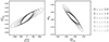 |
Fig. B.3. Impact of z > 1 clusters in survey A on fNL |
All Tables
Impact of measurement errors on the constraints provided by surveys A and B, and eRASS:8.
All Figures
|
Fig. 1. Integrated CR (blue) and S/N profiles (pink) of a cluster at the detection limit at z = 2 for survey B. This cluster has a mass of M500c = 3.9 × 10¹³ h−1 M⊙, and a core radius of rc = 5.04″. Its total count rate is CR∞ = 4.00 × 10⁻³ c s−1. Only a reduced aperture ensures a 5σ detection. This cluster is the detection limit, and so we infer Ropt = 11″ for survey B. Its count rate within the aperture is CR(r < Ropt) = 2.27 × 10⁻³ c s−1, which is just slightly above the CRlim quoted in Table 3. In survey B, about 80 photons, on average, would be collected in total for this cluster. |
| In the text | |
|
Fig. 2. Mass detection limit for surveys A and B. The plain (dashed) lines represent the 50% (10%) detection limit in the M500c − z plane. A given cluster with mass above (below) a line has a detection probability of higher (lower) than 50% in the corresponding survey design. The circles, stars, and triangles denote cluster samples from XXL (Adami et al. 2018), Planck SZ (Planck Collaboration XXVII 2016), and SPT (Bleem et al. 2015), respectively. |
| In the text | |
|
Fig. 3. Number counts for surveys A and B. Survey A has a density of clusters that is about twice the density in B, but the effect of the survey area dominates and B detects twice as many clusters as A (11 200 vs. 5500). |
| In the text | |
|
Fig. 4. Detected cluster populations in the XOD representation. The z–CR–HR diagrams are integrated over the redshift dimension here. The colour scale indicates the number of clusters per pixel (different range for surveys A and B). |
| In the text | |
|
Fig. 5. Comparison of the constraints on Ωm, σ8 for ΛCDM provided by surveys A and B. |
| In the text | |
|
Fig. 6. Survey B constraints for ΛCDM from the 0 < z < 1 (orange) and 1 < z < 2 (cyan) subsamples, and combination of the low-z scaling relation information with the 1 < z < 2 subsample (blue). The full analysis is shown in red. |
| In the text | |
|
Fig. 7. Impact of z > 1 clusters in survey B on Ωm, σ8 for ΛCDM. The outer and faintest ellipse corresponds to the analysis restricted to the 0.05 < z < 1 range. Each successive inner and darker ellipse extends the analysis to higher redshift, up to z = 2. |
| In the text | |
|
Fig. 8. Comparison of the constraints on w0, wa, Ωm, and σ8 for wzCDM provided by surveys A and B. |
| In the text | |
|
Fig. 9. Survey B constraints for wzCDM from the 0 < z < 1 (orange) and 1 < z < 2 (cyan) subsamples, and when adding the low-z scaling relation information to the 1 < z < 2 subsample (blue). The full analysis is shown in red. |
| In the text | |
|
Fig. 10. Impact of z > 1 clusters in survey B on w0, wa, Ωm, and σ8 for wzCDM. The outer and fainter ellipse corresponds to the analysis restricted to the 0.05 < z < 1 range, and the successive inner and darker ellipses extend the analysis to higher redshift, up to z = 2. |
| In the text | |
|
Fig. 11. Comparison of constraints on fNL, Ωm, and σ8 provided by surveys A and B for local primordial non-Gaussianities (cluster counts only). |
| In the text | |
|
Fig. 12. Impact of the z > 1 clusters in survey B on fNL, Ωm, and σ8 for local primordial non-Gaussianities (cluster counts only). The outer and fainter ellipse corresponds to the analysis restricted to the 0.05 < z < 1 range, and the successive inner and darker ellipses extend the analysis out to z = 2. |
| In the text | |
|
Fig. 13. Constraints on σ8(z) (top panel) and fσ8 (bottom panel) from independent redshift bins in survey B. For comparison, we show current constraints from DES 3 × 2pt (DES Collaboration 2023) and eBOSS (Alam et al. 2021). |
| In the text | |
|
Fig. 14. Constraints on fNL from individual redshift bins in survey B (points). The dotted line shows the constraint of all redshift bins combined together, and the histogram represents the number counts. |
| In the text | |
|
Fig. 15. Difference between fiducial diagrams for surveys A (left) and B (right) with and without the measurement errors. The differences are rescaled as a fraction of the maximum value of the fiducial without errors. |
| In the text | |
|
Fig. B.1. Impact of z > 1 clusters in survey A on w0, wa |
| In the text | |
|
Fig. B.2. Impact of z > 1 clusters in survey A on Ωm, σ8 |
| In the text | |
|
Fig. B.3. Impact of z > 1 clusters in survey A on fNL |
| In the text | |
Current usage metrics show cumulative count of Article Views (full-text article views including HTML views, PDF and ePub downloads, according to the available data) and Abstracts Views on Vision4Press platform.
Data correspond to usage on the plateform after 2015. The current usage metrics is available 48-96 hours after online publication and is updated daily on week days.
Initial download of the metrics may take a while.