| Issue |
A&A
Volume 663, July 2022
|
|
|---|---|---|
| Article Number | A3 | |
| Number of page(s) | 18 | |
| Section | Cosmology (including clusters of galaxies) | |
| DOI | https://doi.org/10.1051/0004-6361/202141204 | |
| Published online | 01 July 2022 | |
The XXL survey
XLVI. Forward cosmological analysis of the C1 cluster sample
1
AIM, CEA, CNRS, Université Paris-Saclay, Université Paris Diderot, Sorbonne Paris Cité, 91191 Gif-sur-Yvette, France
e-mail: This email address is being protected from spambots. You need JavaScript enabled to view it.
2
Institut de Physique Théorique, CEA Saclay, 91191 Gif-sur-Yvette, France
3
Department of Astronomy, University of Geneva, Ch. d’Écogia 16, 1290 Versoix, Switzerland
4
Dipartimento di Fisica e Astronomia “Augusto Righi” – Alma Mater Studiorum Università di Bologna, Via Piero Gobetti 93/2, 40129 Bologna, Italy
5
INAF – Osservatorio di Astrofisica e Scienza dello Spazio di Bologna, Via Piero Gobetti 93/3, 40129 Bologna, Italy
6
INFN, Sezione di Bologna, viale Berti Pichat 6/2, 40127 Bologna, Italy
7
Dipartimento di Fisica, Università degli Studi Roma Tre, Via della Vasca Navale 84, 00146 Rome, Italy
8
Argelander Institut für Astronomie, Universität Bonn, 53121 Bonn, Germany
9
IRAP, Université de Toulouse, CNRS, UPS, CNES, 31028 Toulouse, France
10
Academia Sinica Institute of Astronomy and Astrophysics (ASIAA), No. 1, Section 4, Roosevelt Road, Taipei 10617, Taiwan
11
Aix Marseille Univ., CNRS, CNES, LAM, Marseille, France
12
INAF – IASF Milan, Via A. Corti 12, 20133 Milano, Italy
13
Institute for Astronomy and Astrophysics, Space Applications and Remote Sensing, National Observatory of Athens, 15236 Palaia Penteli, Greece
14
CEA Saclay, DRF/Irfu/DEDIP/LILAS, 91191 Gif-sur-Yvette Cedex, France
15
National Observatory of Athens, 11810 Thessio, Greece
16
Physics Department, Aristotle University of Thessaloniki, 51124 Thessaloniki, Greece
Received:
28
April
2021
Accepted:
23
September
2021
Abstract
Context. We present the forward cosmological analysis of an XMM-selected sample of galaxy clusters out to a redshift of unity. We derive mass-observable relations in a self-consistent manner using the sample alone. Special care is given to the modelling of selection effects.
Aims. Following our previous 2018 study based on the dn/dz quantity alone, we perform an upgraded cosmological analysis of the same XXL C1 cluster catalogue (178 objects), with a detailed account of the systematic errors. The results are combined with external constraints from baryon acoustic oscillations (BAO) and the cosmic microwave background (CMB).
Methods. This study follows the ASpiX methodology: we analysed the distribution of the observed X-ray properties of the cluster population in a 3D observable space (count rate, hardness ratio, redshift) and modelled as a function of cosmology along with the scaling relations and the selection function. Compared to more traditional methods, ASpiX allows the inclusion of clusters down to a few tens of photons and is much simpler to use. Two M − T relations are considered: that from the Canada-France-Hawaii Telescope (hereafter CFHT) and another from the more recent Subaru lensing analyses.
Results. We obtain an improvement by a factor of two compared to the previous analysis, which dealt with the cluster redshift distribution for the XXL sample alone, letting the normalisation of the M − T relation and the evolution of the L–T relation free. Adding constraints from the XXL cluster two-point correlation function and the BAO from various surveys decreases the uncertainties by 23% and 53%, respectively, and 62% when adding both. The central value is in excellent agreement with the Planck CMB constraints. Switching to the scaling relations from the Subaru analysis and leaving more parameters free to vary provides less stringent constraints, but those obtained are still consistent with the Planck CMB at the 1-sigma level. Our final constraints are  ,
,  ) for the XXL sample alone. Combining XXL ASpiX, the XXL cluster two-point correlation function, and the BAO, leaving 11 parameters free to vary, and allowing for the cosmological dependence of the scaling relations in the fit induces a shift of the central values, which is reminiscent of that observed for the Planck S-Z cluster sample. We find
  and
and  ), which are still compatible with Planck CMB at 2.2σ.
Conclusions. The results obtained by the ASpiX method are promising; further improvement is expected from the final XXL cosmological analysis involving a cluster sample that is twice as large. Such a study paves the way for the analysis of the eROSITA and future Athena surveys.
Key words: surveys / X-rays: galaxies: clusters / cosmological parameters
© C. Garrel et al. 2022
 Open Access article, published by EDP Sciences, under the terms of the Creative Commons Attribution License (https://creativecommons.org/licenses/by/4.0), which permits unrestricted use, distribution, and reproduction in any medium, provided the original work is properly cited.
1. Introduction
As the largest gravitationally collapsed objects in the Universe, clusters of galaxies occupy a privileged position in astrophysical studies for two main reasons. The cluster number counts and spatial distribution of galaxy clusters as a function of mass and redshift are sensitive to both the growth of structure and the geometry of the Universe, and therefore these objects constitute powerful cosmological probes. While the purely gravitational aspect is theoretically well understood, the interplay between the three cluster components, namely galaxies (∼5%), gas (∼15%) and dark matter (∼80%), renders the physics of the intracluster medium (ICM) complex. A wide range of phenomena are involved: cooling through X-ray emission, enrichment and heating of gas through supernovae and AGN feedback, turbulence, and magnetic fields (see e.g., review by Allen et al. 2011). These processes make clusters interesting astrophysical laboratories and have motivated considerable computational efforts to reproduce their properties using hydrodynamic simulations (e.g., review by Borgani & Kravtsov 2011). The modelling of these properties is crucial in linking cluster observables like galaxy richness, velocity dispersion, gas mass, X-ray luminosity, and temperature (LX, TX) to the total cluster mass, a key component for cosmological studies.
In this context, a Very Large XMM programme was allocated in 2010: with its two spatially disconnected regions of 25 deg2 each, the XXL survey was specifically designed to obtain robust cosmological constraints from the X-ray cluster population out to a redshift of unity. This survey is accompanied by an extensive multi-wavelength follow-up programme and has motivated the development of sophisticated detection and analysis procedures (Pierre et al. 2016, hereafter XXL Paper I). We refer the reader to this latter paper for a comprehensive bibliographical overview of cosmological X-ray cluster surveys. In the construction of the XXL cluster sample, two aspects were given special attention: (i) The cluster selection is solely described in terms of observed X-ray parameters: by selecting clusters in the two-dimensional count-rate versus apparent-size parameter space, we can ensure a sample purity of better than 95% and whose definition is independent of the cosmology. (ii) The cluster scaling relations entering the cosmological analysis are derived from the cluster sample data alone.
A first cosmological analysis of the brightest XXL clusters (the C1 sample containing 178 objects) was presented in Pacaud et al. (2018, hereafter XXL Paper XXV). This study, based on the modelling of the cluster redshift distribution (dn/dz), provided constraints on σ8 and Ωm with precision of the order of 10% and 20%, respectively. No cluster mass information was propagated in the analysis other than the resulting mass detection limit as a function of redshift and cosmology. A natural follow-up would be the subsequent analysis of the dn/dM/dz distribution, which is theoretically much more constraining than dn/dz. However, because the direct handling of the (cosmology-dependent) masses is difficult, we adopted a forward modelling based on the prediction of directly observable quantities; namely, the three-dimensional distribution of the count rates (CRs), hardness ratios (HRs), and redshifts of the selected cluster population (X-ray observable diagrams, hereafter XOD). This method (named ASpiX) was initiated by Clerc et al. (2012a,b) and further validated on analytical and numerical simulations (Pierre et al. 2017; Valotti et al. 2018). ASpiX is intrinsically equivalent to the study of the mass–redshift distribution because the mass information is encoded in the CR–HR–z distribution, but ASpiX is much simpler to use and is less affected by physics or cosmology degeneracies. The method consists in comparing the observed XOD with the predicted XODs as a function of cosmology and cluster evolutionary physics. In the present study, the comparison is performed adopting a Markov chain Monte-Carlo (MCMC) approach, in which selections of cosmological parameters and scaling relation coefficients are left free to vary; the predicted XOD are convolved by a realistic measurement error model.
The paper is organised as follows. Section 2 briefly recalls the main properties of the cluster sample. In Sect. 3, we describe the steps involved in the XOD construction. In Sect. 4 we present a first cosmological analysis under exactly the same hypotheses as in XXL Paper XXV; this allows a direct comparison of the two approaches. We further add constraints from the two-point correlation function from the same cluster sample. In Sect. 5, we update the study by using the revised scaling relations obtained from our recent lensing analysis of deep Hyper Suprime Camera images. The results, along with various sources of uncertainty, are discussed in Sect. 6 with constraints from other probes. Conclusions are drawn in Sect. 7. Appendix A describes the procedure used to measure the cluster quantities appearing in the XOD. Appendix B gives the details of the cosmological likelihood calculation in the CR–HR space, including the estimate of the sample variance.
Throughout the paper, we assume a spatially flat Λ cold dark matter (ΛCDM) model (see Sect. 4). We use the standard notation MΔ to denote the cluster mass enclosed within a sphere of radius rΔ, within which the mean overdensity is equal to Δ times the critical density of the Universe at a particular redshift z.
2. Cluster sample
The present paper deals with a sample of 178 XXL C1 clusters detected in the 47.36 deg2 XXL survey. This is identical to the sample used in the previous XXL cosmological analysis (XXL Paper XXV). In this section, we recall the properties of this sample and describe the measurements of the cluster parameters used in the current study.
2.1. Sample
Adami et al. (2018), hereafter XXL Paper XX, published a sample of 365 clusters divided into two classes, namely the C1 and C2 class. The C1 subsample consists of 191 sources, achieving a high degree of purity (fewer than 5% of the point sources are misclassified as extended; Pacaud et al. 2006). We restricted the cosmological analysis to only the C1 spectroscopically confirmed clusters within the [0.05−1] redshift range. This led to the exclusion of 8 clusters that were outside of the redshift range and 5 without redshift estimates, resulting in a final sample of 178 clusters. In the present study, each cluster is characterised by four observable parameters: redshift (z), X-ray count rate (CR; defined as the number of X-ray counts received per second in the [0.5−2] keV energy band normalised to its on-axis value), hardness ratio (HR; defined as the ratio between the count rates in the [1−2] and [0.5−1] keV energy bands), and angular core radius (θc, assuming a β-profile with β = 2/3; Cavaliere & Fusco-Femiano 1976, 1978); CR and HR are equivalent to physical flux and colour. The CR–HR distribution of the XXL C1 sample is shown in Fig. 1.
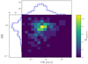 |
Fig. 1. X-ray observable diagram (XOD) of the XXL C1 sample containing 178 objects, integrated over the [0.05−1] redshift range. The blue histograms show the 1D integrated CR and HR distributions. Error bars only account for shot noise. |
2.2. Measurements
Along with a precise mapping of the selection function, the ASpiX method requires robust measurements of the CR and HR quantities with realistic error estimates. We describe the adopted procedure below.
The XXL detection pipeline (XAMIN; Pacaud et al. 2006) operates on the [0.5−2] keV images and provides a list of sources; a multi-PSF fit returns the source extent (θc) for the extended source model, and the resulting CR. The X-ray pipeline also provides the pixel segmentation mask for each source from the first detection pass. The fitted CR and θc values are ascribed measurement likelihoods by XAMIN, but errors are not provided for these quantities. In all that follows, the XAMIN output is used to deal with cluster selection issues only.
In order to obtain model-independent CR measurements along with associated errors, we apply a novel method based on Monte-Carlo sampling to fit the X-ray profile (pyproffit; Eckert et al. 2020) on the mosaic of overlapped XMM observations. Based on a multi-scale profile decomposition, this method allows robust CR and therefore HR measurements, together with an estimate of their uncertainties. Given that the mean number of collected photons per cluster is low (on average ∼200 counts for 10 ks exposures), we use a simplified minimisation algorithm for the θc measurements. The complete procedure is detailed in Appendix A.
3. Cosmological modelling
The main goal of the paper is to perform a forward cosmological analysis: the ASpiX method consists of fitting the CR − HR − z XOD. This approach was tested on simulations and described in a series of articles (Clerc et al. 2012a,b; Pierre et al. 2017; Valotti et al. 2018). In this section, we recall the principles and assumptions inherent to the method.
3.1. ASpiX method
Starting from a theoretical mass function, ASpiX reconstructs the XOD of a given cosmological-plus-cluster-physics model in order to match the observed XOD. The strength of this method is in the fact that it only relies on strictly observable X-ray parameters, which means that the cluster temperatures, luminosities, and masses are not explicitly computed.
We start from the differential mass function computed for a given cosmology, and expressed in terms of redshift (z) and sky area (Ω) folded with the XXL survey effective sky coverage. We compute the distribution in terms of MΔ, z and cluster characteristic size:
 (1)
(1)
where rΔ is the radius within which the average density is Δ times ρc, the critical density.
We use scaling relations linking mass and temperature [MΔ–T], luminosity and temperature [L–T], and between rΔ and the cluster core radius rc, assuming a β model with β = 2/3, [rc–rΔ]. The relation between physical and apparent core radii reads:
![Mathematical equation: $$ \begin{aligned} \theta _{\rm c} \mathrm{\ [arcsec]} = \frac{648\,000}{\pi } r_{\rm c} \mathrm {\ [Mpc]} \ /\ d_{a}(z) \mathrm {\ [Mpc]} , \end{aligned} $$](/articles/aa/full_html/2022/07/aa41204-21/aa41204-21-eq6.gif) (2)
(2)
where da is the angular diameter distance.
We make use of the APEC model: the emission spectrum from collisionally ionised diffuse gas is calculated from the ATOMDB atomic database, (Smith et al. 2001) with a metallicity of 0.3 Z⊙. Folding the spectrum with the EPIC (European Photon Imaging Camera) XMM response matrices provides us with count rates in the three energy bands of interest ([0.5−2] keV, [0.5−1] keV and [1−2] keV). From this, we subsequently construct the 4D z–CR–HR–θc diagram.
We stress that the mass information is implicitly encrypted in the θc, CR, and HR parameters via the scaling relations. We then apply the XXL survey selection function (f[CR,θc]) and finally convolve the XOD with the measurement-error model of each observable parameter except for z (spectroscopically measured and thus with negligible error). In the end, we integrate over θc to obtain the 3D z–CR–HR diagram expected for a given cosmology.
3.2. Assumptions and numerical inputs
For the purpose of this analysis, we use a Tinker mass function (Tinker et al. 2008) computed at an overdensity of Δ = 500. We disperse over the luminosity, temperature and core radius distributions by including a log-normal scatter around the mean scaling relations. The binning of the XOD is shown in Table 1.
Sampling of the X-ray parameter distribution in the XOD.
3.2.1. Scaling relations
In the first part of the paper, in order to allow a direct comparison of the different methodologies applied, we continue to use the scaling relations of XXL Paper XXV modelled, as usual, by power laws:
 (3)
(3)
 (4)
(4)
 (5)
(5)
where M500, WL is the weak-lensing mass estimate within r500, T300 kpc is the cluster X-ray temperature measured inside 300 kpc,  is the luminosity within r500 in the [0.5−2] keV energy band, and E(z) is the redshift evolution of the Hubble parameter, E(z)≡H(z)/H0. The mass calibration only relies on weak lensing measurements based on the Canada-France-Hawaii Telescope (CFHT) lensing data (for a didactic review of cluster weak lensing, see Umetsu 2020). The scaling law parameters are summarised in Table 2.
Cluster scaling laws used in the first part of the paper.
During the analysis, two scaling relation parameters were introduced as nuisance parameters and marginalised. These parameters correspond to the ones indicated by uncertainties in Table 2. We do not include any scatter in the rc − r500 and M500, WL–T300 kpc relations within the base model so that comparisons can be made with XXL Paper XXV. Subsequently, we add a scatter of 0.1 in the rc − r500 in Sect. 5 to correspond to the updated scaling relations. We discuss the impact of larger values of the scatter in Sect. 6.3.
3.2.2. Selection function
Assuming a circular β = 2/3 model for extended sources, a cluster population with different count-rates and θc was generated for a range of XMM exposures. This process takes into account the instrumental characteristics (PSF distortion, vignetting, detector masks, background, and Poisson noise) for the three XMM detectors. Point sources are added at random over the XMM field of view, with a flux distribution following the log(N)−log(S) from Moretti et al. (2003) down to 5 × 10⁻¹⁶ erg s−1 cm−2; the contribution of point sources below 4 × 10⁻¹⁵ erg s−1 cm−2 is included in the cosmic background component (Read & Ponman 2003). The XXL cluster-detection algorithm is then applied, allowing a statistical study to determine various levels of completeness and purity. The cluster selection is performed in the XAMIN output parameter space (EXT, EXT_STAT) and subsequently translated into the CR–θc plane. The details of the procedure are given in Pacaud et al. (2006). The XXL C1 selection function, matched to the XXL exposure and background maps, is shown in Fig. 2.
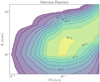 |
Fig. 2. XXL C1 selection function used in this analysis. From simulations of XMM cluster observations, the detection probability is expressed as a function of only observable quantities: the count rate and the apparent size of a β = 2/3 model, θc. The same selection function was used in XXL Paper XXV. |
We stress that the selection function is mapped back into the intrinsic CR–θc space (the probability of detecting a cluster that has these parameters, and not the pipeline ones measured at those values); there is therefore no inconsistency in using CR values for the cosmological analysis that were measured using the pyproffit package.
3.2.3. Measurement errors
As shown in Clerc et al. (2012b), the inclusion of measurement errors changes the shape of the predicted X-ray observable diagrams. A precise estimate of the measurement errors is therefore a key step in the analysis.
The pyproffit package provides us with error estimates for each measurement. This allows us to subsequently model the relative measurement errors on CR, HR, and θc as a function of CR and θc using the following parametrisation:
 (6)
(6)
The choice of the CR–θc plane is a natural second-order approximation reflecting the fact that, physically, the brighter and more peaked a cluster, the better the measurement.
We perform a non-linear least square fit using the Levenberg-Marquardt algorithm (Levenberg 1944; Marquardt 1963) in order to constrain the {ax}, {bx}, and {cx} coefficients. The resulting error models are shown in Fig. 3 and the coefficients are given in Table 3.
 |
Fig. 3. Relative error model (in percent) for each observable used in this analysis. These models are computed as a function of CR and θc. |
3.2.4. Likelihood
The log-likelihood model used to infer the cosmological parameters is given, for each redshift bin, by1:
 (7)
(7)
where  is the number of predicted clusters in the (CRj, HRj) 2D bin (and
  the number of predicted clusters in the redshift bin i) and
  is the number of observed clusters. Here,
  is the mean galaxy cluster bias for the 2D bin j, and
  is the mean bias of the survey (see Eqs. (B.9) and (B.10) of Appendix B). To calculate these quantities, we use the Tinker et al. (2010) bias model.
  is the variance of the total number density contrast. Then, in Eq. (7), the first line is the usual shot-noise term and the second and third lines are the sample-variance terms. Finally,
 (8)
(8)
Following the formalism presented in Valageas et al. (2011), we estimate that the sample variance value is ∼30% of the Poisson variance.
The cosmological parameters are constrained using a MCMC procedure by an affine-invariant ensemble (Goodman & Weare 2010), following the EMCEE algorithm (Foreman-Mackey et al. 2013). In order to optimise computation time while having enough statistics to control the chain convergence, we ran five independent chains in parallel, each with 2N walkers, with N specifying the number of free parameters. The chains are stopped when reaching the Gelman-Rubin convergence criterion of R − 1 < 0.03, after excluding a 20% burn-in phase.
4. Cosmological analysis with the scaling relations of XXL Paper XXV
We assume a flat ΛCDM model. We perform the Monte Carlo analysis and create contour plots by means of the GETDIST Python package (Lewis 2019). The displayed 1σ and 2σ confidence intervals show respectively the 68% and 95% limits.
4.1. XXL ASpiX alone
In this section, we present the cosmological constraints obtained from the XOD alone. We consider five free cosmological parameters within the ΛCDM framework: {Ωm, σ8, Ωb, ns, h}. Two scaling relation parameters are included as nuisance parameters: the M − T normalisation (X0, M − T), and the L − T evolution index (γL − T) as summarised in Table 2; this already allows for significant freedom in the parametrisation of cluster physics unknowns and related cosmological dependence. These two parameters are marginalised during the Monte Carlo analysis.
We apply conservative Gaussian priors for the cosmological parameters which are not well constrained by cluster counts (namely Ωb and ns). These are centred on the Planck-2018 (Planck Collaboration VI 2020) values with errors multiplied by a factor of five in order not to force the agreement between our results and the Planck ones, i.e.: Ωb = 0.0493 ± 0.0035, ns = 0.9649 ± 0.022. The prior on the Hubble constant is chosen to be uniform within a [0.55−0.9] range.
We choose two different methods to estimate the improvement (or deterioration) in the parameter constraints in the Ωm − σ8 plane:
We first use Green’s theorem to compute the area, by line integral, inside the 1σ contours in the Ωm − σ8 plane for two different probes. Taking the square root of the ratio of these two areas gives us the estimated gain or loss in constraining power in the Ωm − σ8 plane.
We also quantify this improvement using a figure of merit (FoM) defined as  where CovΩm − σ8 denotes the covariance matrix.
While keeping the same sample and scaling relations as in XXL Paper XXV, the ASpiX method allows us to improve constraints in the Ωm − σ8 plane by a factor of approximately two. This improvement was not unexpected because the [CR, HR, z] combination is comparable to the mass information, which did not enter the first XXL cosmological analysis, which was based on only dn/dz.
We note that, even though the XXL Paper XXV results, Planck constraints, and our new constraints are all compatible at the 2σ level (0.7σ posterior agreement2 in the Ωm − σ8 plane between XXL ASpiX and XXL Paper XXV), our central values now show better agreement with the Planck results. We find  versus 0.3165 ± 0.0085 for Planck, σ8 = 0.829 ± 0.048 versus 0.8119 ± 0.0074, and S8 = 0.882 ± 0.046 versus 0.834 ± 0.016 for Planck, leading to a 0.4σ posterior agreement in the Ωm − σ8 plane. The results are summarised in Table 4. The Ωm − σ8 contours are shown in Fig. 4 along with recent constraints from other cosmological probes.
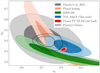 |
Fig. 4. Ωm − σ8 cosmological constraints from XXL ASpiX (this work), Planck-2018 (Planck TT TE EE lowl lowE), Planck S-Z cluster counts (Planck15 Cluster), Planck lensing (CMB lensing potential analysis; Planck Collaboration VIII 2020), KIDS-450 (tomographic weak gravitational lensing of the 450 deg2 Kilo Degree Survey; Hildebrandt et al. 2017) and the previous XXL cosmological results, XXL Paper XXV (Pacaud et al. 2018). |
ASpiX cosmological constraints for the base model and the joint analysis (flat ΛCDM).
4.2. XXL ASpiX + XXL clustering
Cosmological constraints from the 3D clustering analysis of the XXL cluster sample (two-point correlation function, 2PCF) were presented in Marulli et al. (2018). In this section, we combine the 2PCF and ASpiX results.
In order to perform the joint analysis, we run the MCMC procedure as before, and use the XXL 2PCF mean and covariance results as additional priors for all the parameters that are left free during the analysis, namely: {Ωm, σ8, Ωb, ns, h, τ}. The 2PCF study was performed using seven free parameters, the six above-mentioned cosmological parameters and, in addition, the effective bias of the cluster sample, beff (see Marulli et al. 2018, for the detailed procedure).
We model the (redshift dependent) effective sample bias following Matarrese et al. (1997):
 (9)
(9)
and we define the averaged effective bias of the sample as:
 (10)
(10)
where 𝒩(z, M) is the number of clusters with mass M and redshift z as predicted by a given cosmological scenario (including the selection effects), and b(M, z) is the dark matter halos bias computed using the Tinker et al. (2010) model for M500.
While beff is free during the XXL clustering analysis, it is an output of the cluster counts (or ASpiX) analysis and depends on the selection function in the M − z space. The selection function in the M − z space depends, in turn, on the cosmology and the scaling relations. We therefore implement the results for beff from the XXL clustering analysis as an additional Gaussian term in the likelihood from Eq. (7).
The results are shown in Table 4. The Ωm − σ8 contours are shown in Fig. 5. The joint XXL ASpiX + 2PCF analysis reduces the uncertainties on Ωm and σ8 by 23% (figure of merit (FoM) increased by a factor of 1.3) compared to ASpiX alone. The Ωm result is slightly lower, Ωm = 0.314 ± 0.031, and σ8 slightly higher, σ8 = 0.840 ± 0.044, and with  . Nevertheless, the results are still in good agreement with Planck CMB.
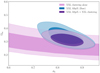 |
Fig. 5. The Ωm − σ8 cosmological constraints of XXL ASpiX cluster counts alone (base), XXL 2PCF (clustering alone), and of the joint analysis. |
4.3. XXL clusters + BAO joint analysis
In this section, we combine the ASpiX constraints with those obtained from baryon acoustic oscillation (BAO) measurements of clustering of galaxies. The BAO data used in this analysis are reported in Table 5. We describe the adopted methodology and present the results from the joint analysis.
BAO data used in this analysis.
We use two quantities to model the BAO distance measurements: (i) the spherically averaged distance,
![Mathematical equation: $$ \begin{aligned} D_{V}(z) = \left[ (1+z)^2 d_{a}^2(z) \frac{cz}{H(z)} \right]^{\frac{1}{3}} , \end{aligned} $$](/articles/aa/full_html/2022/07/aa41204-21/aa41204-21-eq37.gif) (11)
(11)
and (ii) the sound horizon at the drag epoch (Eisenstein & Hu 1998),
![Mathematical equation: $$ \begin{aligned} r_s(z_d) = \frac{2}{3 k_{\rm eq}}\sqrt{\frac{6}{R(z_{\rm eq})}}\ ln \left[ \frac{\sqrt{1+R(z_d)} + \sqrt{R(z_d) + R(z_{\rm eq})}}{1 + \sqrt{R(z_{\rm eq})}} \right] , \end{aligned} $$](/articles/aa/full_html/2022/07/aa41204-21/aa41204-21-eq38.gif) (12)
(12)
where zd is the redshift at the drag epoch, zeq is the matter-radiation equality redshift, keq is the scale of the particle horizon at the equality epoch, and R(z) is the ratio of the baryon to photon momentum density at redshift z. We model these four quantities following Eisenstein & Hu (1998) (with a CMB temperature of 2.725 K). The BAO distance is then given by
 (13)
(13)
where  is the sound horizon computed for a chosen fiducial cosmology (see Table 5). The likelihood is therefore modified by adding a Gaussian log-likelihood term in Eq. (7) :
![Mathematical equation: $$ \begin{aligned} \mathcal{L}_{\rm BAO}&= \frac{1}{2} \sum _i \left[ \frac{\mathcal{D} ^\mathrm{th}(z_i) - \mathcal{D} ^\mathrm{set\ I}_i}{\sigma _{\mathcal{D} ^\mathrm{set\ I}_i}} \right]^2\nonumber \\&+\frac{1}{2} \left[ \boldsymbol{\mathcal{D} }^\mathrm{th} - \boldsymbol{\mathcal{D} }^\mathrm{set\ II}\right] C^{-1}_{\rm WiggleZ} \left[ \boldsymbol{\mathcal{D} }^\mathrm{th} - \boldsymbol{\mathcal{D} }^\mathrm{set\ II}\right] , \end{aligned} $$](/articles/aa/full_html/2022/07/aa41204-21/aa41204-21-eq41.gif) (14)
(14)
where the inverse covariance matrix,  , comes from the fact that the three WiggleZ measurements are correlated (see Table 4 of Kazin et al. 2014).
Combining the BAO and the XXL 2PCF decreases the uncertainties by 62% (FoM increased by a factor of 2.6) and confirms the agreement with Planck (Ωm = 0.317 ± 0.017,  and
and  ). The results are shown in Table 4. The Ωm − σ8 contours are shown in Fig. 6.
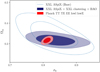 |
Fig. 6. Ωm − σ8 constraints obtained by XXL ASpiX alone (base) and XXL ASpiX + XXL clustering + BAO analysis and Planck-2018 (Planck TT TE EE lowl lowE). |
4.4. XXL ASpiX + Planck CMB
In this section, we combine our results with those of Planck-2018 (CMB anisotropy measurement) by means of importance sampling. The results are shown in Table 4. The Ωm − σ8 contours are shown in Fig. 7.
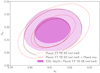 |
Fig. 7. Comparison between Planck CMB + XXL ASpiX and Planck CMB + Planck lens and Planck CMB alone in terms of the Ωm − σ8 constraints. |
By combining our results with those of Planck-2018 (CMB anisotropies measurement) we reduce Planck uncertainties by 30% (FoM increased by a factor of 1.4) on Ωm and σ8 and find good agreement with the constraints from the combination of Planck-2018 and Planck lensing (lensing potential analysis of the temperature and polarisation data); see Fig. 6. We note that the XXL + Planck-2018 combination yields constraints comparable to those provided by the Planck-2018 + Planck lensing combination.
5. Cosmological modelling with updated scaling relations
Two independent mass-observable studies (Eckert et al. 2016, hereafter XXL Paper XIII, and Umetsu et al. 2020) suggest that cluster masses were overestimated in our first analysis based on the CFHT lensing data (XXL Paper IV). In this section, we rerun the cosmological analysis, assuming our newly determined scaling relations from the joint XXL-HSC (Hyper Suprime-Cam Survey) analysis by Umetsu et al. (2020) and Sereno et al. (2020).
For this purpose, we follow the formalism of Umetsu et al. (2020) for the scaling relations.
We consider the cluster true mass M500, True as the fundamental property of galaxy clusters for the T − M relation and we use the weak lensing mass M500, WL as a mass proxy.
Umetsu et al. (2020) characterised the weak lensing mass bias as a function of true cluster mass using cosmological N-body simulations (the dark-matter-only run from the BAHAMAS project; McCarthy et al. 2017, 2018). These authors estimated that, at the typical mass for the XXL sample (M500 = 7 × 10¹³h−1 M⊙), the bias is approximately −11%. We therefore apply a correction for the weak lensing mass bias by assuming a constant of −11%:
 (15)
(15)
with
 (16)
(16)
and we assume a Gaussian prior on log10(1 + bWL) of log10(1 + bWL) = log10(1 − 0.11)±5%/ln10 to marginalise over the mass calibration uncertainty of ±5%, see Umetsu et al. (2020). Here σlog10MWL in Eq. (16) is the intrinsic scatter of weak-lensing mass at fixed true cluster mass, M500, True.
The L − T relation is given by:
 (17)
(17)
and we keep Eq. (5) for the relation between rc and r500.
We fit the coefficients of the T − M and L − T relations (namely : {X0, T − M, X0, L − T, αT − M, αL − T, γT − M, γL − T, σT − M, σlog10MWL, σL − T}, with σT − M/L − T the log-normal intrinsic scatters) using the publicly available LIRA package (Sereno 2016a,b) for the XXL C1 sample (using the procedure and measurements described in Sereno et al. 2020 and Umetsu et al. 2020). The results, computed for Ωm = 0.28 and h = 0.7 in a flat ΛCDM universe, are shown in Table 6.
The effective impact of the cosmological dependence3 of weak lensing mass measurements and luminosities is expected to be small given the parameter range considered and the statistical and systematic errors inherent to our cluster sample. Nevertheless, to ensure better consistency, we model the effect of cosmology on the scaling relations a posteriori as follows:
-
We use an analytical approximation (Sereno 2015) to account for the dependence of the lensing mass on cosmology:
 (18)
(18)where Dl, Ds, and Dls are the lens, the source, and the lens-source angular diameter distances respectively. In a first approximation, we assume a linear relation between the cluster redshift and mean redshift of the source galaxies:
 (19)
(19)This results in a mean source–galaxy redshift of 1 for a cluster at 0.3 and of 1.5 for a cluster at redshift 1. We use δγ = 0.196, fitted on our C1 sample, to rescale the masses on a grid of Ωm and h values. The ranges are defined to be Ωm ∈ [0.1 − 0.8] and h ∈ [0.5 − 0.9], with a step of 0.1 for each parameter. This provides us with the masses for 40 combinations of Ωm − h values. We then compute the T–M scaling relation for each [Ωm − h] point of the grid to obtain the corresponding mean values and covariance matrices.
-
Masses from the M–T relations are used to rescale r500 (r500, rescale); we then extrapolate the luminosities within r500, rescale assuming a β-profile with a core radius rc = 0.15 r500, rescale and a slope β = 2/3. Finally, luminosities are normalised by the correction factor
 . This procedure provides us with rescaled luminosities for the 40 combinations of Ωm − h values. We then compute the L–T scaling relation for each Ωm − h point of the grid to obtain corresponding mean values and covariance matrices.
 -
Here, the cosmological analysis deals with five free cosmological parameters : {Ωm, σ8, Ωb, ns, h} plus six free scaling relation parameters: {X0, T − M, X0, L − T, αT − M, αL − T, γT − M, γL − T}. In the MCMC, the values of the six scaling relation parameters are limited through adaptive Gaussian priors by interpolating the means and covariance matrices over the grid of 40 combinations of Ωm − h values.
-
We disperse temperatures and luminosities; these scatters are assumed to be independent of cosmology. We moreover introduce a log-normal scatter in the rc − r500 relation.
Resulting constraints on Ωm − σ8 (we refer to this model as XXL-HSC ASpiX) are shown in Fig. 8 and compared with the results of Sect. 4.1 (referring to this model as the base model). The constraints when adding the XXL 2PCF and BAO measurements are shown in Fig. 9. All the results are shown in Table 7.
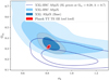 |
Fig. 8. Impact of thawing parameters in the scaling relations. XXL ASpiX (base) refers to the results presented in Sect. 4.1 (two free scaling parameters); XXL-HSC ASpiX contours are the results following the methodology presented in Sect. 5 (six free cosmology-dependent scaling parameters); simple dark blue contours, same as XXL-HSC but the priors of the scaling coefficients are fixed to the indicated cosmology. We can see that, in this case, the results in Ωm − σ8 are shifted (lower Ωm and higher σ8) because of the fact that the scaling relation priors do not depend on the cosmology and then introduce a bias in the analysis. |
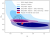 |
Fig. 9. Same as Fig. 8 when adding constraints from XXL clustering and external BAO. The dashed line stands for the case where only two scaling coefficients are let free. |
ASpiX cosmological constraints for the HSC-XXL ASpiX model and the joint analysis (flat ΛCDM).
For XXL-HSC ASpiX, we find slightly higher Ωm and σ8 results and with larger error bars,  ,
,  (
( ). Nevertheless, the results are compatible at the 1-σ level with our base model and the Planck CMB. Furthermore, because our uncertainties are now larger, we are compatible with the Planck S-Z cluster counts as well.
Adding the XXL clustering, we find a smaller Ωm = 0.296 ± 0.034 and a higher  (
( ), which are fully consistent with the findings of Planck CMB at the 1-sigma level.
Combining XXL-HSC ASpiX with the XXL clustering and the BAO measurements, the results are shifted (Ωm = 0.364 ± 0.015,  ,
,  ) and we find results in better agreement with the Planck S-Z cluster sample while remaining consistent with Planck CMB at 2.2σ.
6. Discussion
6.1. Summary of results
Figure 4 shows that, as expected, the constraints on Ωm − σ8 have improved by more than a factor of two with respect to XXL Paper XXV under exactly the same hypotheses. This confirms, on real data, the power of the ASpiX forward modelling in terms of simplicity and accuracy. The size of the error bars is now comparable to that from the Planck S-Z cluster sample (Planck Collaboration XXIV 2016). At this point, it is important to recall that the Planck cluster sample contains almost three times as many clusters as XXL, that these clusters are much more massive, and that the XXL scaling relations do not rely on external cluster calibration samples or on hydrodynamical simulations, contrary to those of Planck; currently, the two data sets are still consistent at the 2-σ level, even though the favoured XXL cosmology is closer to the Planck CMB values. Combining the ASpiX constraints with the results from the cluster–cluster correlation function from the same sample improves the constraints by 23% (Fig. 5), and by 62 % (Fig. 6) when adding both cluster–cluster correlation function and BAO measurements.
In a second step, we reran the ASpiX analysis by implementing the updated scaling relations along with a modelling of their cosmological dependence, that is, by increasing the degrees of freedom on cluster physics from two to six (Fig. 8 and Table 6). As expected, this results in larger error bars: we now favour a higher σ8 value,  , but this is still compatible at the 1-σ with the results of the Planck CMB.
At this stage, we are close to having exhausted the cosmological information contained in the current data set relative to the XXL C1 cluster sample. It is instructive to review and discuss the various possible sources of systematic error that impinge upon these new results and, thus, assess their robustness.
A number of possible systematic uncertainties were already identified and discussed in the previous cosmological analysis of XXL Paper XXV. In the following section, we review further hypotheses and examine the impact on the initial base model. To quantify the robustness of our results, we analyse the posterior distribution of the S8 = σ8(Ωm/0.3)0.5 product.
6.2. Impact of error model
To study the impact of the error model, we arbitrarily modify the true error model by increasing errors by 20% and 50%, and we monitor the effect on the cosmological constraints (referring to them as Error + 20% and Error + 50% respectively).
We can see from Fig. 10 that increasing the relative measurement errors increases the uncertainty on S8 slightly, without any drastic change in the mean result. Nevertheless, the general pattern seems to indicate that assuming excessive measurement errors tends to decrease S8. The agreement between models is shown in Table 8.
6.3. Scaling relation model
We now investigate how the results are impacted by different scaling relation models. First, we present the results when only adding a scatter of 0.5 in the rc − r500 relation. We then study the effect of adding scatter in the M − T relation.
Hereafter, we refer to the 0.5 scatter in the rc − r500 relation as the σ0.5, rc − r500 model. In Fig. 10, we can see that adding a 50% scatter in the rc − r500 relation favours a slightly higher S8 value while increasing the uncertainties by only 3% compared to the base model. All in all, the results appear little affected (Table 8). If we had added θc as the fourth dimension in the XOD and used it in the cosmological inference, the error bars would probably be smaller, but more dependent on the scatter value (cf. Valotti et al. 2018).
In the base model, we did not implement a scatter in the M − T relation to keep the same configuration as in XXL Paper XXV (all scatter is supposed to be encapsulated in L − T). However, because HR directly depends on cluster temperature, it is logical to include a dispersion. We then include a 0.41 scatter in the M − T relation obtained from XXL Paper IV. We refer to this model from now on as σ0.41, M − T.
This model is in good agreement with the base one with a significance level of posterior agreement in the Ωm − σ8 − Ωb − ns space of 0.1σ and 0.3σ in the Ωm − σ8 plane; see Table 8 and Fig. 10.
6.4. Impact on Ωb priors
To ensure that the prior chosen for Ωb is not too restrictive, we apply a Gaussian prior centred on the Planck 2018 values but with errors multiplied by a factor of 20 : Ωb = 0.0493 ± 0.015 (i.e. our previous prior multiplied by 4). We refer to this model from now on as ‘Ωb prior × 4’.
The resulting constraint on S8 is shown in Fig. 10 and the agreement between models in Table 8.
We find that the results are fully consistent with the base model (0.02σ posteriors agreement in 4D Ωm − σ8 − Ωb − ns space and 0.04σ posteriors agreement in Ωm − σ8 only, see Table 8). In conclusion, because Ωb prior × 4 becomes computationally expensive, we determine that it is relevant to keep the base model prior for Ωb.
6.5. Error on the selection function
In this section, we study the impact of uncertainties on the selection function. This is a priori a key issue because an ill-determined selection directly biases the modelling of the cluster number counts. Currently, our selection is based on simulations assuming spherically symmetric and β = 2/3 profiles for the cluster emission. To quantify the impact of a poorly monitored cluster selection on the cosmological inference, we degrade the selection function; i.e. we blur the current function displayed in Fig. 2 by a 2D adaptive Gaussian filter characterised by:
 (20)
(20)
As easily understandable, in this way, fainter and smaller clusters are more affected. We refer to this modelling from now on as Selfunc * Gauss.
The Selfunc * Gauss result on S8 is shown in Fig. 10 and the agreement between models is shown in Table 8. While increasing uncertainties on S8, the blurred selection function also lowers the mean S8 value.
6.6. Remaining sources of uncertainty
In addition to the sources of systematic uncertainty reviewed above, we also note the main assumptions used in the course of the present study. Firstly, the covariance between the observable parameters (CR, HR, and θc) is neglected; the model has been slightly extrapolated in order to account for objects scattered out or in the measured domain. Furthermore, we do not consider the covariance between the scatters of the M–T and L–T scaling relations. In both cases, the scatter is assumed to be independent of the underlying cosmology. In the lensing analysis, we assume a linear relation between lens cluster redshift and the galaxy source photometric redshifts as stated in Eq. (19). Finally, we restrict our analysis to only one particular mass function (Sect. 3.2) for this study. We aim to examine the impact of these assumptions in the subsequent and final XXL analysis – consisting of a larger number of clusters – in order to determine the most accurate, unbiased cosmological estimates from the XXL sample.
7. Conclusions
Following Clerc et al. (2012b) and simulation case studies, we present the first application of the ASpiX cosmological forward modelling on real data with redshift information. The outcome confirms the flexibility and efficiency of the method. The constraints obtained from the 178 XXL C1 clusters, under various hypotheses, yield a precision comparable to that of the current BAO and Planck S-Z samples, as shown in Fig. 9. Nevertheless, the number of degrees of freedom left in the analysis reflects the accuracy of the recovered cosmological parameters, which is most easily seen when comparing the XXL base model alone (dashed blue contours) to the tightest constraints from this analysis (purple contours).
In short, the current results present an improvement by a factor of two compared to the preceding dn/dz analysis of the same sample. At this stage, we may recall the final cosmological modelling of the REFLEX survey number counts. This latter is based on the luminosity function of more than 800 clusters detected in the ROSAT All-Sky Survey (z < 0.4; Böhringer et al. 2014). Our base model analysis (Sect. 4.1) on the 178 C1 clusters includes four free cosmological parameters plus two scaling relation coefficients as nuisance parameters; in the REFLEX analysis, only the slope of the M–L relation was left free to vary free and it was assumed that the luminosity function does not evolve. Under these conditions, we find a precision on Ωm comparable to that of REFLEX but almost twice better for σ8; both parameter sets being compatible within the error bars.
Another cosmological analysis of RASS clusters was conducted as part of the ‘Weighing the Giants’ project. The 224 ‘Giants’ are massive clusters spanning the 0 < z < 0.3 redshift range. Gas masses from deep ROSAT and Chandra observations were subsequently derived for 94 of them. Independent mass calibration was achieved by weak gravitational lensing for 27 of these. This enabled the derivation of uniquely well-defined scaling relations and subsequently yielded a precision of the order of 5% on σ8 and Ωm (with standard priors on Ωb, h, and ns fixed; Mantz et al. 2015). Constraints are tighter than with the XXL clusters, but it is important to recall here that the only X-ray information used in the current study is the XMM 10ks survey data, which means a median number of photons of about 200 per cluster. We can anticipate that devoting very large amounts of X-ray follow-up time to the XXL clusters would lead to significant improvement on the WtG constraints thanks to the wider redshift range spanned by the XXL clusters.
Ultimately, the XXL XMM observation set will be reprocessed at full depth by running the detection algorithm on the mosaicked data (Faccioli et al. 2018, hereafter XXL Paper XXIV). This will not only increase the sensitivity but also the surveyed area, because the current cluster catalogue (XXL Paper XX) was extracted only from the single pointings, restricted to an off-axis distance of 13 arcminutes. It is therefore expected that the final XXL cosmological release will involve a sample twice as large as the current one, with a deeper C1 and C2 population. In the subsequent cosmological analysis, we shall add information from the third X-ray observable, the apparent core radius (Valotti et al. 2018). The final cosmological sample should bring an improvement of a factor of approximately 1.5 − 2 on the present constraints.
Using the same sample of 178 clusters, our next study will focus on the w parameter of the ΛCDM model. To this purpose, we shall make use of the HSC full depth information on the background galaxy photometric redshifts; the cosmological dependence of the cluster lensing masses will be rescaled as a function of w. The inclusion of the cluster two-point correlation function, while having little effect on the current study which is limited to Ωm and σ8, is expected to reduce the uncertainty on w by a factor of two (Pierre et al. 2011). Similarly, we shall allow for more flexibility in the determination of the cluster selection function: by considering a range of cluster ellipticities and quantifying the impact of cool cores or central AGN in the detection, we will be in a position to assess systematic uncertainties more precisely.
Because photometric redshifts are almost as efficient as spectroscopic redshifts in ASpiX (Clerc et al. 2012a), the application of the method to the upcoming eROSITA cluster sample should readily reveal most of the cosmological potential of the eROSITA sample.
See Appendix B for its formal derivation.
To compute the agreement between two different probes, we rely on the following process. We first draw a representative sample for each posterior of interest from the two probes. We compute the distance between each pair of points of these samples. We build, from this distance sample, the probability distribution using kernel density estimate. We then estimate the probability to exceed (PTE) by integrating the probability distribution over the interval [0-P(0)], with P(0) the probability of a distance equal to zero. The same formalism is used in Bocquet et al. (2019). The corresponding significance level is computed assuming Gaussian statistics. To insure that the results are not impacted by randomisation effects, we repeat this process one hundred times and present the mean significance level.
On Ωm and h, for a flat ΛCDM model.
Acknowledgments
XXL is an international project based around an XMM Very Large Programme surveying two 25 deg2 extragalactic fields at a depth of ∼6 × 10⁻¹⁵ erg cm−2 s−1 in the [0.5–2] keV band for point-like sources. The XXL website is http://irfu.cea.fr/xxl. The Saclay team acknowledges long term support from the Centre National d’Etudes Spatiales. This work was supported by the Programme National Cosmology et Galaxies (PNCG) of CNRS/INSU with INP and IN2P3, co-funded by CEA and CNES. MS acknowledges financial contribution from contract ASI-INAF n.2017-14-H.0 and INAF ‘Call per interventi aggiuntivi a sostegno della ricerca di main stream di INAF’. LM acknowledges the grants PRIN-MIUR 2017 WSCC32 and ASI-INAF n. 2018-23-HH.0. KU acknowledges support from the Ministry of Science and Technology of Taiwan (grants MOST 106-2628-M-001-003-MY3 and MOST 109-2112-M-001-018-MY3) and from the Academia Sinica Investigator Award (grant no. AS-IA-107-M01). Finally, the authors would like to thanks the referee for the useful comments.
References
- Adami, C., Giles, P., Koulouridis, E., et al. 2018, A&A, 620, A5 (XXL Paper XX) [NASA ADS] [CrossRef] [EDP Sciences] [Google Scholar]
- Alam, S., Ata, M., Bailey, S., et al. 2017, MNRAS, 470, 2617 [Google Scholar]
- Allen, S. W., Evrard, A. E., & Mantz, A. B. 2011, ARA&A, 49, 409 [Google Scholar]
- Beutler, F., Blake, C., Colless, M., et al. 2011, MNRAS, 416, 3017 [NASA ADS] [CrossRef] [Google Scholar]
- Bocquet, S., Dietrich, J. P., Schrabback, T., et al. 2019, ApJ, 878, 55 [Google Scholar]
- Böhringer, H., Chon, G., & Collins, C. A. 2014, A&A, 570, A31 [NASA ADS] [CrossRef] [EDP Sciences] [Google Scholar]
- Borgani, S., & Kravtsov, A. 2011, Adv. Sci. Lett., 4, 204 [Google Scholar]
- Cash, W. 1979, ApJ, 228, 939 [Google Scholar]
- Cavaliere, A., & Fusco-Femiano, R. 1976, A&A, 49, 137 [NASA ADS] [Google Scholar]
- Cavaliere, A., & Fusco-Femiano, R. 1978, A&A, 70, 677 [NASA ADS] [Google Scholar]
- Clerc, N., Pierre, M., Pacaud, F., & Sadibekova, T. 2012a, MNRAS, 423, 3545 [NASA ADS] [CrossRef] [Google Scholar]
- Clerc, N., Sadibekova, T., Pierre, M., et al. 2012b, MNRAS, 423, 3561 [NASA ADS] [CrossRef] [Google Scholar]
- Dembinski, H., Ongmongkolkul, P., Deil, C., et al. 2020, https://doi.org/10.5281/zenodo.3949207 [Google Scholar]
- Eckert, D., Ettori, S., Coupon, J., et al. 2016, A&A, 592, A12 (XXL Paper XIII) [NASA ADS] [CrossRef] [EDP Sciences] [Google Scholar]
- Eckert, D., Finoguenov, A., Ghirardini, V., et al. 2020, Open J. Astrophys., 3, 12 [NASA ADS] [CrossRef] [Google Scholar]
- Eisenstein, D. J., & Hu, W. 1998, ApJ, 496, 605 [Google Scholar]
- Faccioli, L., Pacaud, F., Sauvageot, J. L., et al. 2018, A&A, 620, A9 (XXL Paper XXIV) [NASA ADS] [CrossRef] [EDP Sciences] [Google Scholar]
- Foreman-Mackey, D., Hogg, D. W., Lang, D., & Goodman, J. 2013, PASP, 125, 306 [Google Scholar]
- Goodman, J., & Weare, J. 2010, Commun. Appl. Math. Comput. Sci., 5, 65 [Google Scholar]
- Hildebrandt, H., Viola, M., Heymans, C., et al. 2017, MNRAS, 465, 1454 [Google Scholar]
- Hoffman, M. D., & Gelman, A. 2011, ArXiv e-prints [arXiv:1111.4246] [Google Scholar]
- Kazin, E. A., Koda, J., Blake, C., et al. 2014, MNRAS, 441, 3524 [NASA ADS] [CrossRef] [Google Scholar]
- Levenberg, K. 1944, Quart. Appl. Math., 2, 164 [Google Scholar]
- Lewis, A. 2019, ArXiv e-prints [arXiv:1910.13970] [Google Scholar]
- Lieu, M., Smith, G. P., Giles, P. A., et al. 2016, A&A, 592, A4 (XXL Paper IV) [NASA ADS] [CrossRef] [EDP Sciences] [Google Scholar]
- Mantz, A. B., von der Linden, A., Allen, S. W., et al. 2015, MNRAS, 446, 2205 [Google Scholar]
- Marquardt, D. W. 1963, J. Soc. Ind. Appl. Math., 11, 431 [Google Scholar]
- Marulli, F., Veropalumbo, A., Sereno, M., et al. 2018, A&A, 620, A1 [NASA ADS] [CrossRef] [EDP Sciences] [Google Scholar]
- Matarrese, S., Coles, P., Lucchin, F., & Moscardini, L. 1997, MNRAS, 286, 115 [NASA ADS] [CrossRef] [Google Scholar]
- McCarthy, I. G., Schaye, J., Bird, S., & Le Brun, A. M. C. 2017, MNRAS, 465, 2936 [Google Scholar]
- McCarthy, I. G., Bird, S., Schaye, J., et al. 2018, MNRAS, 476, 2999 [NASA ADS] [CrossRef] [Google Scholar]
- Moretti, A., Campana, S., Lazzati, D., & Tagliaferri, G. 2003, ApJ, 588, 696 [NASA ADS] [CrossRef] [Google Scholar]
- Pacaud, F., Pierre, M., Refregier, A., et al. 2006, MNRAS, 372, 578 [NASA ADS] [CrossRef] [Google Scholar]
- Pacaud, F., Pierre, M., Melin, J. B., et al. 2018, A&A, 620, A10 (XXL Paper XXV) [NASA ADS] [CrossRef] [EDP Sciences] [Google Scholar]
- Padmanabhan, N., Xu, X., Eisenstein, D. J., et al. 2012, MNRAS, 427, 2132 [Google Scholar]
- Pierre, M., Pacaud, F., Juin, J. B., et al. 2011, MNRAS, 414, 1732 [Google Scholar]
- Pierre, M., Pacaud, F., Adami, C., et al. 2016, A&A, 592, A1 (XXL Paper I) [NASA ADS] [CrossRef] [EDP Sciences] [Google Scholar]
- Pierre, M., Valotti, A., Faccioli, L., et al. 2017, A&A, 607, A123 [NASA ADS] [CrossRef] [EDP Sciences] [Google Scholar]
- Planck Collaboration XXIV. 2016, A&A, 594, A24 [NASA ADS] [CrossRef] [EDP Sciences] [Google Scholar]
- Planck Collaboration VI. 2020, A&A, 641, A6 [NASA ADS] [CrossRef] [EDP Sciences] [Google Scholar]
- Planck Collaboration VIII. 2020, A&A, 641, A8 [NASA ADS] [CrossRef] [EDP Sciences] [Google Scholar]
- Read, A. M., & Ponman, T. J. 2003, A&A, 409, 395 [NASA ADS] [CrossRef] [EDP Sciences] [Google Scholar]
- Ross, A. J., Samushia, L., Howlett, C., et al. 2015, MNRAS, 449, 835 [NASA ADS] [CrossRef] [Google Scholar]
- Sereno, M. 2015, MNRAS, 450, 3665 [Google Scholar]
- Sereno, M. 2016a, MNRAS, 455, 2149 [Google Scholar]
- Sereno, M. 2016b, LIRA: LInear Regression in Astronomy Astrophysics Source Code Library [record ascl:1602.006] [Google Scholar]
- Sereno, M., Umetsu, K., Ettori, S., et al. 2020, MNRAS, 492, 4528 [CrossRef] [Google Scholar]
- Smith, R. K., Brickhouse, N. S., Liedahl, D. A., & Raymond, J. C. 2001, ApJ, 556, L91 [Google Scholar]
- Tinker, J., Kravtsov, A. V., Klypin, A., et al. 2008, ApJ, 688, 709 [Google Scholar]
- Tinker, J. L., Robertson, B. E., Kravtsov, A. V., et al. 2010, ApJ, 724, 878 [NASA ADS] [CrossRef] [Google Scholar]
- Umetsu, K. 2020, A&ARv, 28, 7 [Google Scholar]
- Umetsu, K., Sereno, M., Lieu, M., et al. 2020, ApJ, 890, 148 [NASA ADS] [CrossRef] [Google Scholar]
- Valageas, P., Clerc, N., Pacaud, F., & Pierre, M. 2011, A&A, 536, A95 [NASA ADS] [CrossRef] [EDP Sciences] [Google Scholar]
- Valotti, A., Pierre, M., Farahi, A., et al. 2018, A&A, 614, A72 [NASA ADS] [CrossRef] [EDP Sciences] [Google Scholar]
Appendix A: X-ray parameter measurements
The use of the XOD for cosmology requires accurate measurements along with realistic error estimates. In this section, we provide details on the various steps of the X-ray analysis for single clusters. Measurements are performed on the mosaicked co-added observations.
A.1. Step 1: Manually monitoring θbkg
We use the interactive fluxmes procedure (Clerc et al. 2012b) to determine the cluster-centric distance from which the background can be safely estimated (θbkg). In addition, this procedure allows us to check that all neighbouring sources have been correctly flagged by the pipeline; and possibly to re-adjust the corresponding masks. The fluxmes application is based on a curve of growth analysis and decides where to set the ‘no man’s land limit’ around the cluster. In the following, the particle background is measured using a very large number of ‘closed-filter’ observations, scaled to our XXL observations using the detector parts not exposed to the sky (corners); this results in two 25 deg2 maps, corresponding to the mosaicked observations and exposure maps. The astrophysical background (passing through the XMM optics) is locally estimated in the [θbkg, 15 arcmin] annulus around each cluster in the course of the pyproffit procedure (see Sec. A.3).
A.2. Step 2: The θc measurements
Given that cluster angular sizes directly intervene in the selection (Fig. 2), we need to determine the apparent core radii along with associated uncertainties. This is performed under the hypothesis of a β = 2/3 model, as used to determine the selection function by means of simulations (Pacaud et al. 2006). The convolution by the PSF assumes a mean function over the entire mosaic (a cluster is generally seen at several off-axis positions on different observations):
![Mathematical equation: $$ \begin{aligned} \mathrm{PSF} (\theta _{on-axis}) = \left[1+\left(\frac{\theta _{on-axis}}{4.765^{\prime \prime }}\right)^2\right]^{-1.505}, \end{aligned} $$](/articles/aa/full_html/2022/07/aa41204-21/aa41204-21-eq69.gif) (A.1)
(A.1)
where θon − axis is the angular radius (on-axis). The fit is performed for each cluster on the [0.5-2] keV co-added XMM mosaic and includes the corresponding exposure and background maps; the neighbouring sources are removed from the data using the revised masks. We use iminuit (Dembinski et al. 2020) to fit the Cash log-likelihood (Cash 1979).
A.3. Step 3: Accurate count-rate measurements
The last step is to obtain best count-rate measurements along with realistic uncertainties for the three X-ray bands involved in the construction of the XOD (Sec. 2). To optimise the determination, we relax the hypothesis of a single β = 2/3 model and rather model the cluster emission by a linear combination of β-profiles following the pyproffit methodology (Eckert et al. 2020):
 (A.2)
(A.2)
where Nℱ is the total number of functions and αi the model coefficients. {ℱi} is defined (Eckert et al. 2016) as
![Mathematical equation: $$ \begin{aligned} \mathcal{F} _i(\theta ) = \left[1+\left(\frac{\theta }{\theta _{c,i}}\right)^2\right]^{-3\beta _i+1/2} , \end{aligned} $$](/articles/aa/full_html/2022/07/aa41204-21/aa41204-21-eq71.gif) (A.3)
(A.3)
where θ is the distance to the cluster centre. The mean value of predicted counts (λ) in profile annulus a is given by
 (A.4)
(A.4)
Practically, we consider six β values within [0.6-3] and N = θbkg/5″ values for θc. The set of coefficients {αi} in equation A.2 that maximises the log-likelihood given by equation A.5, namely
 (A.5)
(A.5)
will describe the best-fit profile.
Eventually, we obtain the reconstructed profile by drawing 1000 posterior samples using No-U-Turn Sampler, NUTS (Hoffman & Gelman 2011). From this profile sample, we draw the count-rate posterior distribution. The various steps of the whole procedure are illustrated in Fig. A.1; for further technical details we refer the reader to (Eckert et al. 2020).
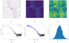 |
Fig. A.1. Example of cluster count-rate measurement with the pyproffit method. The displayed cluster is XLSSC 093 at a redshift of 0.429. (a) X-ray mosaic around the cluster; the image is 30 arcmin aside. (b) Particle background map. (c) Combined exposure map along with the masks hiding the neighbouring sources. (d) Extracted cluster profile (black crosses); the green line displays the particle background level extracted from map (b): this component is already subtracted from the displayed profile. (e) Overlaid on the extracted profile, the reconstructed (PSF-deconvolved) profile is shown in blue along with the 1-σ estimated uncertainty. (f) Count-rate posterior distribution (MOS1 normalised) of the reconstructed profile. |
Appendix B: Likelihood
B.1. Probability distribution of galaxy clusters in the (z, CR, HR) space
We describe the distribution of X-ray clusters as a Poisson realisation of an underlying continuous field. Thus, the number of observed clusters  in the bin i, in the 3D space (zi, CRi, HRi) (or any other set of observables) follows the Poisson probability distribution
 (B.1)
(B.1)
where  is the continuous cluster density field. This continuous field
  is also a random variable because of the sample variance, following the fluctuations of the dark matter density field averaged over the survey volume. It is given by
![Mathematical equation: $$ \begin{aligned} \hat{n}_i = \int _{z_{i-}}^{z_{i+}} dz \frac{d\chi }{dz} \mathcal{D}^2 \int d{\boldsymbol{\Omega }} \int d\ln M \frac{d\hat{n}}{d\ln M} \Theta _i[M,z], \end{aligned} $$](/articles/aa/full_html/2022/07/aa41204-21/aa41204-21-eq78.gif) (B.2)
(B.2)
with
![Mathematical equation: $$ \begin{aligned} \Theta _i[M,z]&= \int _{-\infty }^{\infty } \frac{d\epsilon _{\rm CR}}{\sqrt{2\pi } \sigma _{\rm CR}} e^{-\epsilon ^2_{\rm CR}/(2 \sigma ^2_{\rm CR})} \int _{-\infty }^{\infty } \frac{d\epsilon _{\rm HR}}{\sqrt{2\pi } \sigma _{\rm HR}} \nonumber \\&\times e^{-\epsilon ^2_{\rm HR}/(2 \sigma ^2_{\rm HR})} \nonumber \\&\times \Theta ( \mathrm{CR}_{i-} < f_{\rm CR}(M,z)+\epsilon _{\rm CR} < \mathrm{CR}_{i+} ) \nonumber \\&\times \Theta ( \mathrm{HR}_{i-} < f_{\rm HR}(M,z)+\epsilon _{\rm HR} < \mathrm{HR}_{i+} ). \end{aligned} $$](/articles/aa/full_html/2022/07/aa41204-21/aa41204-21-eq79.gif) (B.3)
(B.3)
Here, fCR(M, z) is the count rate associated with a cluster of mass M at redshift z, with a Gaussian scatter σCR. In practice, we can use a lognormal scatter by considering lnCR as our observable, or by replacing the Gaussian integral in (B.3) by a lognormal distribution. Then, the first factor Θ is a unit top-hat that is non-zero when the count rate falls in the bin i. Similar notations are used for the hardness ratio. Thus, Θi[M, z] is the probability that a cluster of mass M at redshift z falls in the 2D bin (CRi, HRi). In Eq.(B.2) we integrate the number of clusters over the redshift bin Δzi = zi+ − zi−, the survey angular area ΔΩ, and the cluster mass M, where χ and 𝒟 are the radial and angular comoving distances and  is the observed cluster mass function. Selection effects are included in the mass function
  , which differs from the halo mass function and contains the response of the instrument.
At the level of the continuous field, the mean number of clusters in the bin i is
![Mathematical equation: $$ \begin{aligned} \bar{n}_i \equiv \langle \hat{n}_i \rangle = \Delta \Omega \int _{z_{i-}}^{z_{i+}} dz \frac{d\chi }{dz} \mathcal{D}^2 \int d\ln M \frac{d n}{d\ln M} \Theta _i[M,z] , \end{aligned} $$](/articles/aa/full_html/2022/07/aa41204-21/aa41204-21-eq82.gif) (B.4)
(B.4)
where  is the cluster mass function predicted by a given cosmological scenario (including the selection effects). If we neglect sample variance, we take
  without any scatter, and the Poisson distribution (B.1) has the fixed mean
  . This provides the shot-noise contribution to the measurement error bars that is associated with the discreteness of the cluster distribution.
To estimate the impact of the sample variance, we consider the covariance of the continuous number counts  . We have
![Mathematical equation: $$ \begin{aligned} C_{ij}&\equiv \langle \hat{n}_i \hat{n}_j \rangle - \langle \hat{n}_i \rangle \langle \hat{n}_j \rangle \nonumber \\&= \int d\chi _1 d{\boldsymbol{\Omega }}_1 d\ln M_1 \int d\chi _2 d{\boldsymbol{\Omega }}_2 d\ln M_2 \mathcal{D}_1^2 \mathcal{D}_2^2 \Theta _i[M_1,z_1] \nonumber \\&\times \Theta _j[M_2,z_2] \frac{dn}{d\ln M}(M_1,z_1) \frac{dn}{d\ln M}(M_2,z_2) \xi _{12}({\boldsymbol{x}}_1-{\boldsymbol{x}}_2), \end{aligned} $$](/articles/aa/full_html/2022/07/aa41204-21/aa41204-21-eq87.gif) (B.5)
(B.5)
where ξ12 is the two-point correlation of halos with masses of M1 and M2. We assume that the redshift bins are much larger than the correlation length of the clusters and that the correlation function can be factorised as
 (B.6)
(B.6)
where ξ(x) is the dark-matter correlation function and b(M, z) is the bias of clusters of mass M at redshift z. We use the Tinker et al. (2010) bias model during this analysis. Then, neglecting finite-sized effects associated with the borders of the survey volume, we can write the covariance matrix as
 (B.7)
(B.7)
where δzi, zj is the Kronecker symbol with respect to the redshift bins i and j,  is the mean correlation in the redshift bin i, defined by
 (B.8)
(B.8)
and  is the mean bias defined by
![Mathematical equation: $$ \begin{aligned} \bar{n}_i \bar{b}_i = \Delta \Omega \int _{z_{i-}}^{z_{i+}} dz \frac{d\chi }{dz} \mathcal{D}^2 \int d\ln M \frac{d n}{d\ln M} \Theta _i[M,z] b(M,z) . \end{aligned} $$](/articles/aa/full_html/2022/07/aa41204-21/aa41204-21-eq93.gif) (B.9)
(B.9)
Because of the Kronecker redshift factor in the covariance matrix (B.7), different redshift bins are decoupled and we can analyse each redshift bin separately. Therefore, in the following we focus on a single redshift bin and the index j refers only to the 2D bins (CRj, HRj). It is also useful to consider the total number  of clusters in the survey and its continuous counterpart
  . For non-overlapping bins j we have
 (B.10)
Let us define the fluctuations  and
and  of the continuous number counts
  and
and  in the bin j and in the full 2D volume (CR, HR),
 (B.11)
with means and covariances
 (B.12)
and unit correlation coefficients
 (B.13)
This implies that the fluctuations  are linear functions of each other, and we obtain
 (B.14)
This is a consequence of the factorisation (B.6) of the cluster correlation function. We also note  the variance of the total number density contrast in the redshift bin,
 (B.15)
B.2. Mean correlation 
For small angular windows and large enough redshift bins, it is possible to simplify the computation of the mean correlation  defined in Eq.(B.8). In the flat-sky approximation, for circular windows of angular radius θs, this computation reads as
 (B.16)
where χ0 is the comoving radial distance to the median redshift z0 of the bin and P(k, z0) is the matter density power spectrum at redshift z0. For redshift bins that are not too shallow, Δχ ≫ 𝒟θs, the integral over χ along the line of sight suppresses the contributions from parallel wave numbers k∥ > 1/(Δχ), so that  is dominated by transverse wave numbers k⊥ ∼ 1/(𝒟θs) ≫ k‖ and k ≃ k⊥. This is Limber’s approximation in its Fourier form. Then, the integral over χ gives a Dirac factor 2πδD(k∥), and the integration over k∥ yields
 (B.17)
Introducing the 2D Fourier-space circular window W2(k⊥𝒟θs),
 (B.18)
where J1 is the Bessel function of first order and first type, and we obtain
 (B.19)
B.3. Likelihood for the number counts in (CR, HR)
We now extend the likelihood-ratio analysis of Cash (1979) to our case. Denoting θα the parameters of the model, such as the set of cosmological parameters and additional cluster parameters, we consider the likelihood  in the redshift bin zi defined by
 (B.20)
Here we used the fact that the Poisson probabilities  defined in Eq. (B.1) are governed by the continuous number counts nj, which are characterised by their means
  and the fluctuating part δ from Eq.(B.14). The means
  , the bias
  , and the variance
  themselves depend on the cosmological parameters θα. At the level of the second-order moment for δ, assuming the survey is large enough so that the relative fluctuations δ of the total number of clusters in a redshift bin are small, we take P(δ) to be Gaussian so that its probability distribution is fully determined by its variance. This yields
![Mathematical equation: $$ \begin{aligned} L_{z_i}(\theta _\alpha ;\hat{N}_j)&= \int _{-\infty }^{\infty } \frac{d\delta }{\sqrt{2\pi }\sigma _\delta } e^{-\delta ^2/(2\sigma _\delta ^2)} \prod _j \frac{[(1+\frac{\bar{b}_j}{\bar{b}} \delta ) \bar{n}_j ]^{\hat{N}_j}}{\hat{N}_j !} \nonumber \\&\times e^{- (1+\frac{\bar{b}_j}{\bar{b}} \delta ) \bar{n}_j } , \end{aligned} $$](/articles/aa/full_html/2022/07/aa41204-21/aa41204-21-eq122.gif) (B.21)
(B.21)
which also reads as
 (B.22)
Here we used the last property in (B.10). The first product, independent of δ, is the usual shot-noise contribution, whereas the integral over δ of the second product gives the contribution from the sample variance. If the latter is negligible, σδ → 0, it goes to unity and we recover the shot-noise value. If the volume is large enough, the relative fluctuation σδ of the total number of clusters is small and we can expand the logarithm up to second order in δ,
 (B.23)
This is valid if we have
 (B.24)
where we write δ = δN/N and  . For large survey sizes, with N ≫ 1, we typically expect
  so that the approximation (B.23) is valid. We can then perform the Gaussian integration in Eq.(B.22), which gives
![Mathematical equation: $$ \begin{aligned}&L_{z_i}(\theta _\alpha ;\hat{N}_j) = \prod _j \frac{\bar{n}_j^{\hat{N}_j}}{\hat{N}_j !} e^{-\bar{n}_j} \left( 1+\sigma ^2_\delta \sum _j \hat{N}_j \frac{\bar{b}_j^2}{\bar{b}^2} \right)^{-1/2}\nonumber \\&\times \, \exp \left[ \frac{\sigma _\delta ^2}{2} \left( \sum _j \hat{N}_j \frac{\bar{b}_j}{\bar{b}} - \bar{n} \right)^2 \left( 1+\sigma ^2_\delta \sum _j \hat{N}_j \frac{\bar{b}_j^2}{\bar{b}^2} \right)^{-1} \right] . \end{aligned} $$](/articles/aa/full_html/2022/07/aa41204-21/aa41204-21-eq128.gif) (B.25)
(B.25)
For the estimation of the cosmological and cluster parameters θα with the likelihood method (Cash 1979), we compare the logarithm ℒ = −lnL obtained for different sets of parameters. The estimated parameters  are those that minimise ℒ and the variation of ℒ with θα provides the confidence intervals, following a χ2 law. Thus, we consider
 (B.26)
where we use  , within a given redshift bin. Following common practice, we discard the term
  because it does not depend on the parameters θα and cancels out in the difference
  . The first term is the usual shot-noise contribution while the other two terms are the sample-variance contribution, which vanishes for σδ → 0. The sums over j only need to run over the bins in the 2D space (CR, HR) that are not empty, as they come with a factor
  . This ensures that the results are not affected if we enlarge the box in the 2D space (CR, HR) to a large volume far beyond the realistic domain, including regions that are always empty.
Going back to the 3D space (z, CR, HR), because the redshift bins are independent, we simply have for the full likelihood
 (B.27)
In practice, the parameters θα should not be far from those derived from previous experiments, such as Planck (for the cosmological parameters). Then, as in the Fisher matrix analysis where we neglect the cosmological dependence of the covariance matrix, we can neglect the dependence on θα of the sample-variance quantities  , which we compute for a reference cosmology labeled by the subscript (0),
  . We then test the cosmological scenario through its predictions for the means
  . This implies that we can discard the second factor in Eq.(B.26), as it does not depend on θα, and write
 (B.28)
B.4. Behaviour of the likelihood ℒ
B.4.1. Cosmology selected by the data
Let us now investigate the behaviour of ℒzi as a function of the theoretical means  . This will provide us some insight into the response of the cosmological parameters θα to the measurements
  , through the associated means
  . Thus, the cosmology selected by the measurement corresponds to the set
  that maximises the likelihood Lzi, i.e. that minimises the negative logarithm ℒzi. For 𝒩 2D bins at redshift zi, this gives the 𝒩 equations
  ,
,
 (B.29)
where we use  and define
 (B.30)
First, we note that if the measurements are equal to the reference predictions, we recover the reference cosmology:
 (B.31)
where we use the sum rules (B.10).
Second, we note that the 𝒩 equations (B.29) admit the solution
 (B.32)
where α is a solution of the single equation
 (B.33)
where we introduce
 (B.34)
We can understand this from the fact that sample-variance fluctuations of the total number of clusters do not affect the relative counts in the different pixels (CRi, HRi), as seen in Eq.(B.14). Therefore, the inferred ratios  are equal to the measured ratios
  . Thus, this likelihood method selects cosmologies that predict the observed distribution profile in the 2D space (CR, HR), up to a uniform rescaling α.
Next, the quadratic equation (B.33) has two solutions,
 (B.35)
with the asymptotic behaviours for σ2 → 0,
 (B.36)
The physical solution is α−, which goes to unity when the sample variance is negligible and we recover the shot-noise likelihood, where the inferred cosmological values are  .
.
The second solution α+ is not physical and this is due to the approximations in our treatment, such as (B.23). Indeed, it would correspond to a large uniform density fluctuation δ ≃ −1, where the approximation (B.23) is no longer valid. In practice, α+ does not appear and does not impair the likelihood algorithm because we restrict the search in the cosmological parameter space to a small realistic region not too far from the Planck values (i.e. we do not consider cosmologies that would predict ten times more clusters or further than the Planck concordance cosmology).
We can see from Eq.(B.33) that α = 1 is a solution if  . This leads to a generalisation of the solution (B.31),
 (B.37)
which applies for any β > 0. Therefore, if the measurements  follow the same 2D profile as the reference cosmology, up to a uniform multiplicative factor β, there is no rescaling and the likelihood method selects cosmologies that predict the same number counts
  as those that are measured.
If  , we can see from Eq.(B.36) that α < 1. Therefore, the likelihood selects cosmologies that predict mean counts
  that are lower than the measured values
  , and the required increase up to
  is explained by a local positive fluctuation δ > 0 of the density field arising from a sample-variance effect. This can be understood from the fact that
  means that higher-bias pixels have a greater count than expected. This points towards positive density fluctuations δ > 0. This is similar to the well-known Kaiser derivation of the bias of rare objects like clusters, with respect to the underlying dark-matter density field. There, using for instance the Press-Schechter mass function or the peak formalism, it is noted that positive large-scale matter density fluctuations δ > 0 enhance the formation of rare massive objects, and the more extreme the object (i.e. a larger mass) the greater the enhancement. This means a larger bias for more massive halos, because of the increased sensitivity of the large-mass tail of the mass function. Reversing this picture, we can see that enhanced number counts of rare massive halos, i.e. of high-bias objects, arise from positive fluctuations of the underlying matter density field.
Therefore, in our case (and more generally),  signals an enhancement of high-bias objects and hence a positive underlying density fluctuation δ > 0. To accommodate this amplification with the observed values
  , the means
  must then be somewhat smaller than the targets
  .
.
In Fig. B.1, we show the XXL C1 sample diagram together with the diagram predicted by our ΛCDM best-fit parameters given in section 4.1. While the diagram predicted by the best-fit parameters follow the peak position and the shape of the observed diagram, we can see that, as expected, in the CR–HR space not dominated by the shot noise,  is smaller than
  .
.
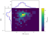 |
Fig. B.1. X-ray observable diagram of the XXL C1 sample, integrated over the redshift range [0.05-1] used in this study, together with the 1D CR, HR distributions in blue. In red, the theoretical diagram predicted by our ΛCDM best-fit parameters given in section 4.1. We can see where the CR–HR space is not dominated by the shot noise ( |


B.4.2. Confidence intervals
We also expect the sample variance to increase the error bars obtained for the parameters θα from the observations, as compared with the shot-noise-only estimate.
From Eq.(B.28) we obtain the Hessian
 (B.38)
We clearly see that the sample-variance contribution decreases the curvature of the likelihood ℒ and therefore increases the size of the confidence interval. For instance, we obtain for the trace and determinant of the Hessian
 (B.39)
 (B.40)
which are decreased by the sample-variance term proportional to σ2. From Eqs.(B.39)-(B.40), we can estimate the change δλj of the eigenvalues λj of the Hessian Hij due to the sample-variance term. With  , λj ∼ λ + δλ, we write
 (B.41)
 (B.42)
For both the trace and the determinant, the comparison with Eqs.(B.39)-(B.40) gives the order-of-magnitude estimate
 (B.43)
where  is the typical number count in a 2D cell. Consequently, we expect the interval of confidence on the cosmological parameters to increase by a factor of the order of
  , when we include the effect of the sample variance. Here
  should correspond to a binning that is well adapted to the survey, that is, which corresponds to the amount of information that can be drawn from the observations. By choosing increasingly small bins, one decreases
  and the apparent magnitude of δλ in Eq.(B.43), but this is compensated by the larger size of the matrix Hjℓ and the greater number of constraints, which are mostly degenerate.
For the likelihood (B.28) to be meaningful, the Hessian H should be positive definite in the neighbourhood of the reference point (0), so that the solutions of Eq.(B.29) correspond indeed to minima of ℒ, and not to local maxima or a saddle points. This requires the determinant (B.40) to be strictly positive. Substituting the expression (B.30), we find that det(H) > 0 if
 (B.44)
This is positive when σδ(0) is small. Moreover, at the reference point, with  , this reads as
 (B.45)
where we use the sum rules (B.10) and we define the averages
 (B.46)
The weights pj are positive and sum to unity. Therefore, they can be interpreted as a probability distribution and we obtain  .
.
Thus, the determinant (B.40) is actually strictly positive at the reference point  for any value of σδ(0). By continuity on σδ(0), this also implies that the Hessian matrix H is always positive definite at this reference point. If the search for the cosmological parameters does not go too far from this reference, the Hessian matrix always remains positive definite. This ensures that the likelihood (B.28) is well behaved.
The Ωm − σ8 constraints from the Log-likelihood of Eq. (B.28) and a simple Poisson Log-Likelihood without sample variance contribution,
 (B.47)
are shown in Fig. B.2.
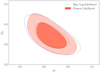 |
Fig. B.2. Ωm − σ8 contours using the log-likelihood from equation B.28 (Base Log-Likelihood) and the Poisson log-likelihood from equation B.47 (Poisson Likelihood). The constraints when using the base log-likelihood compared to the Poisson one are improved by 10%. |
All Tables
ASpiX cosmological constraints for the base model and the joint analysis (flat ΛCDM).
ASpiX cosmological constraints for the HSC-XXL ASpiX model and the joint analysis (flat ΛCDM).
All Figures
|
Fig. 1. X-ray observable diagram (XOD) of the XXL C1 sample containing 178 objects, integrated over the [0.05−1] redshift range. The blue histograms show the 1D integrated CR and HR distributions. Error bars only account for shot noise. |
| In the text | |
|
Fig. 2. XXL C1 selection function used in this analysis. From simulations of XMM cluster observations, the detection probability is expressed as a function of only observable quantities: the count rate and the apparent size of a β = 2/3 model, θc. The same selection function was used in XXL Paper XXV. |
| In the text | |
|
Fig. 3. Relative error model (in percent) for each observable used in this analysis. These models are computed as a function of CR and θc. |
| In the text | |
|
Fig. 4. Ωm − σ8 cosmological constraints from XXL ASpiX (this work), Planck-2018 (Planck TT TE EE lowl lowE), Planck S-Z cluster counts (Planck15 Cluster), Planck lensing (CMB lensing potential analysis; Planck Collaboration VIII 2020), KIDS-450 (tomographic weak gravitational lensing of the 450 deg2 Kilo Degree Survey; Hildebrandt et al. 2017) and the previous XXL cosmological results, XXL Paper XXV (Pacaud et al. 2018). |
| In the text | |
|
Fig. 5. The Ωm − σ8 cosmological constraints of XXL ASpiX cluster counts alone (base), XXL 2PCF (clustering alone), and of the joint analysis. |
| In the text | |
|
Fig. 6. Ωm − σ8 constraints obtained by XXL ASpiX alone (base) and XXL ASpiX + XXL clustering + BAO analysis and Planck-2018 (Planck TT TE EE lowl lowE). |
| In the text | |
|
Fig. 7. Comparison between Planck CMB + XXL ASpiX and Planck CMB + Planck lens and Planck CMB alone in terms of the Ωm − σ8 constraints. |
| In the text | |
|
Fig. 8. Impact of thawing parameters in the scaling relations. XXL ASpiX (base) refers to the results presented in Sect. 4.1 (two free scaling parameters); XXL-HSC ASpiX contours are the results following the methodology presented in Sect. 5 (six free cosmology-dependent scaling parameters); simple dark blue contours, same as XXL-HSC but the priors of the scaling coefficients are fixed to the indicated cosmology. We can see that, in this case, the results in Ωm − σ8 are shifted (lower Ωm and higher σ8) because of the fact that the scaling relation priors do not depend on the cosmology and then introduce a bias in the analysis. |
| In the text | |
|
Fig. 9. Same as Fig. 8 when adding constraints from XXL clustering and external BAO. The dashed line stands for the case where only two scaling coefficients are let free. |
| In the text | |
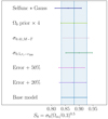 |
Fig. 10. S8 = σ8(Ωm/0.3)0.5 results for all tests discussed in Sect. 6. |
| In the text | |
|
Fig. A.1. Example of cluster count-rate measurement with the pyproffit method. The displayed cluster is XLSSC 093 at a redshift of 0.429. (a) X-ray mosaic around the cluster; the image is 30 arcmin aside. (b) Particle background map. (c) Combined exposure map along with the masks hiding the neighbouring sources. (d) Extracted cluster profile (black crosses); the green line displays the particle background level extracted from map (b): this component is already subtracted from the displayed profile. (e) Overlaid on the extracted profile, the reconstructed (PSF-deconvolved) profile is shown in blue along with the 1-σ estimated uncertainty. (f) Count-rate posterior distribution (MOS1 normalised) of the reconstructed profile. |
| In the text | |
|
Fig. B.1. X-ray observable diagram of the XXL C1 sample, integrated over the redshift range [0.05-1] used in this study, together with the 1D CR, HR distributions in blue. In red, the theoretical diagram predicted by our ΛCDM best-fit parameters given in section 4.1. We can see where the CR–HR space is not dominated by the shot noise ( |
| In the text | |
|
Fig. B.2. Ωm − σ8 contours using the log-likelihood from equation B.28 (Base Log-Likelihood) and the Poisson log-likelihood from equation B.47 (Poisson Likelihood). The constraints when using the base log-likelihood compared to the Poisson one are improved by 10%. |
| In the text | |
Current usage metrics show cumulative count of Article Views (full-text article views including HTML views, PDF and ePub downloads, according to the available data) and Abstracts Views on Vision4Press platform.
Data correspond to usage on the plateform after 2015. The current usage metrics is available 48-96 hours after online publication and is updated daily on week days.
Initial download of the metrics may take a while.