Evidence for non-axisymmetry in M 31 from wide-field kinematics of stars and gas

M. Opitsch; M. H. Fabricius; R. P. Saglia; R. Bender; M. Blaña; O. Gerhard

doi:10.1051/0004-6361/201730597

Home

All issues

Volume 611 (March 2018)

A&A, 611 (2018) A38

Full HTML

Open Access

Issue		A&A Volume 611, March 2018


Article Number		A38
Number of page(s)		22
Section		Extragalactic astronomy
DOI		https://doi.org/10.1051/0004-6361/201730597
Published online		20 March 2018

A&A 611, A38 (2018)

Evidence for non-axisymmetry in M 31 from wide-field kinematics of stars and gas^★,^★★,^★★★

M. Opitsch¹^,2^,3, M. H. Fabricius¹^,2, R. P. Saglia¹^,2, R. Bender²^,1, M. Blaña¹ and O. Gerhard¹

¹ Max Planck Institute for Extraterrestrial Physics, Giessenbachstr., 85748 Garching, Germany
e-mail: mxhf@mpe.mpg.de
² Universitäts-Sternwarte München, Scheinerstr. 1, 81679 Munich, Germany
³ Excellence Cluster Universe, Boltzmannstr. 2, 85748 Garching, Germany

Received: 10 February 2017
Accepted: 14 July 2017

Abstract

Aim. As the nearest large spiral galaxy, M 31 provides a unique opportunity to study the structure and evolutionary history of this galaxy type in great detail. Among the many observing programs aimed at M 31 are microlensing studies, which require good three-dimensional models of the stellar mass distribution. Possible non-axisymmetric structures like a bar need to be taken into account. Due to M 31’s high inclination, the bar is difficult to detect in photometry alone. Therefore, detailed kinematic measurements are needed to constrain the possible existence and position of a bar in M 31.

Methods. We obtained ≈220 separate fields with the optical integral-field unit spectrograph VIRUS-W, covering the whole bulge region of M 31 and parts of the disk. We derived stellar line-of-sight velocity distributions from the stellar absorption lines, as well as velocity distributions and line fluxes of the emission lines Hβ, [O III] and [N I]. Our data supersede any previous study in terms of spatial coverage and spectral resolution.

Results. We find several features that are indicative of a bar in the kinematics of the stars, we see intermediate plateaus in the velocity and the velocity dispersion, and correlation between the higher moment h3 and the velocity. The gas kinematics is highly irregular, but is consistent with non-triaxial streaming motions caused by a bar. The morphology of the gas shows a spiral pattern, with seemingly lower inclination than the stellar disk. We also look at the ionization mechanisms of the gas, which happens mostly through shocks and not through starbursts.

Key words: galaxies: bulges / galaxies: structure / galaxies: kinematics and dynamics / Local Group / techniques: spectroscopic

^★

This paper includes data taken at The McDonald Observatory of The University of Texas at Austin.

^★★

This research was supported by the DFG cluster of excellence “Origin and Structure of the Universe”.

^★★★

Full Tables B.4–B.7 are only available at the CDS via anonymous ftp to cdsarc.u-strasbg.fr (130.79.128.5) or via http://cdsarc.u-strasbg.fr/viz-bin/qcat?J/A+A/611/A38

© ESO 2018

Open Access article, published by EDP Sciences, under the terms of the Creative Commons Attribution License (http://creativecommons.org/licenses/by/4.0;), which permits unrestricted use, distribution, and reproduction in any medium, provided the original work is properly cited.

1 Introduction

Because of its proximity, M 31 is the best case after the Milky Way to learn about the detailed evolutionary history of a large spiral galaxy. Therefore, M 31 has been studied by several major surveys in recent years, combining large-scale photometry with pointed spectroscopic observations. Two of these large programs are the Spectroscopic and Photometric Landscape of Andromeda’s stellar halo survey (SPLASH; Guhathakurta et al. 2005, 2006; Gilbert et al. 2006) and the Pan-Andromeda archaeological survey (PAndAS; McConnachie et al. 2009). These surveys studied the stellar halo of M 31 in great detail, to measure its global properties (Gilbert et al. 2012, 2014) and look at structures within the halo like the Giant Southern Stream (Gilbert et al. 2009). This provided information about the formation history of M 31. One of the results of the PAndAS survey is that white dwarfs galaxies around M 31 all lie in a thin plane (Ibata et al. 2013), which poses problems for the current understanding of galaxy formation. The Panchromatic Hubble Andromeda Treasury (PHAT) program (Dalcanton et al. 2012) looked at the disk of M 31 and obtained photometry for 117 million individual stars (Williams et al. 2014). The Herschel Exploitation of Local Galaxy Andromeda (HELGA; Fritz et al. 2012) observed M 31 in the far infrared and sub-millimeter wavelengths, measuring the distributions of dust (Smith et al. 2012) and molecular clouds (Kirk et al. 2015). Microlensing events and variable stars were monitored by the Pan-STARRS 1 survey of Andromeda (PAndromeda; Lee et al. 2012, 2014a,b). All these surveys help to understand the structure, the accretion history and the history of star formation within M 31.

M 31 is classified as an unbarred spiral SA(s)b by de Vaucouleurs et al. (1991), however, there has been evidence from photometry and kinematics that it is barred, see Sect. 1. In this paper we present new spectroscopic observations of M 31. The paper focusses on the description of the data and the hints for a bar that can be seen there in. A discussion of other possible explanations, like a superposition of disks and rings, goes beyond the scope of this paper and will be presented in future papers based on the dataset described here.

The current Lambda cold dark matter (ΛCDM) paradigm (Planck Collaboration XIII 2016) has been very successful in explaining both the large scale structure of the universe and the observed properties of galaxies. One component of this model is the cold dark matter, which resides in halos around galaxies. The nature of this dark matter is not yet understood. The currently preferred candidates for dark matter are non-baryonic elementary particles, so-called weakly interacting massive particles (WIMPs), see for example Bertone (2010) and references therein. Baryonic candidates for dark matter are mostly ruled out, because the fraction of baryonic matter in the universe is only 15% of the total matter (Planck Collaboration XVI 2014). This baryonic dark matter fraction could be composed of large astrophysical objects, like brown dwarfs, Jupiter-sized planets or black holes, collectively known as massive astrophysical compact halo objects (MACHOs; Griest 1991). In order to place firm constraints on the existence of these massive objects, microlensing studies have been conducted. In such a microlensing event, a MACHO passes between a bright object and the earth, the light from the source objects is deflected by the gravity of the MACHO, which leads to a perceived increase in brightness of the source object. The observation of the frequency of such events allows to determine the number density of MACHOs (Paczynski 1986). The MACHO survey (Alcock et al. 1993) finds that the contribution of MACHOs to the total halo mass of the Milky Way is 20% (Alcock et al. 2000), with an average MACHO mass of ≈0.4 M_⊙. The Expérience pour la Recherche d’Objets Sombres (EROS) and EROS-2 projects (Aubourg et al. 1993; Afonso et al. 2003) measure a significantly lower fraction for the same masses, at less than 8% (Tisserand et al. 2007). The optical gravitational lensing experiment (OGLE; Udalski et al. 1992) finds a fraction that is comparable to the one measured by the EROS-survey (Wyrzykowski et al. 2011), less than 7% for MACHO masses lower than 1 M_⊙ . In addition to these results on the galactic halo, the galactic bulge microlensing surveys within OGLE-III (Wyrzykowski et al. 2015), microlensing observations in astrophysics (MOA) II (Sumi et al. 2013) and EROS-2 (Hamadache et al. 2006) have become major tools for understanding the structure of the Milky Way, see for example Wegg et al. (2016) for a new analysis.

Several microlensing surveys have also been focused toward M 31, like the PAndromeda survey (Lee et al. 2012) and the WendelsteinCalar Alto pixellensing project (WeCAPP; Lee et al. 2015). A total of 56 events have been detected in M 31 (Lee et al. 2015). These events do not have to be caused by MACHOs, they can also happen due to lensing by other stars in M 31, so-called self-lensing (Riffeser et al. 2006). To constrain the number of events that are caused by self-lensing, a proper understanding of the three-dimensional distribution of the stars is needed. Models with different mass distributions of the galaxy result in widely varying predictions of the event rate of self-lensing and lensing through MACHOs. It is therefore important to model the stellar mass distribution in the galaxy as accurately as possible. Based on the data presented in this paper and numerical models from Blaña Díaz et al. (2017, hereafter B17) and Blaña et al. (in prep.), new predictions for microlensing events will be presented in a future paper (Riffeser, in prep.).

A large fraction of disk galaxies in the local universe is barred, ranging from about 50% in the optical (Barazza et al. 2008) to about 60% to 70% in the infrared (Eskridge et al. 2000; Menéndez-Delmestre et al. 2007). It is now thought that global instabilities in the disk lead to the quick formation of bars. In this process, the m = 2 mode grows strongly by swing-amplification and forms a long-lasting bar non-linearly (Sellwood & Wilkinson 1993; Sellwood 2013). Over time, the inner part of the bar goes through a buckling phase, which is a short but violent vertical instability not long after bar formation (Combes & Sanders 1981; Combes et al. 1990; Raha et al. 1991; Merritt & Sellwood 1994; Athanassoula & Misiriotis 2002; Debattista et al. 2005). The instability bends out of the plane of the disk, then settles back to the plane, redistributing energy to smaller spatial scales and to higher stellar velocity dispersion, thereby thickening the bar (Raha et al. 1991). The buckled part of the bar becomes a three-dimensional so-called boxy/peanut shaped (B/P) bulge, the part that has not buckled is referred to as the thin or flat bar. While this buckling phase is frequently seen in simulations, it has only recently been detected in observations by Erwin & Debattista (2016) for two local spiral galaxies.

While the Milky Way was originally thought of as unbarred, it is now widely accepted that it contains a bar. For a review, see Gerhard & Wegg (2015), and references therein. Recently, signs for a bar have also been detected in the innermost parts of the third large spiral galaxy in the Local Group, M 33 (Hernández-López et al. 2009).

The question if M 31 also contains a bar or not has not been settled, for example Widrow et al. (2003) refer to the bulge as “barlike”, while Kormendy et al. (2010) classify M 31 as containing a classical bulge. If present, a bar is not easily detected in images of M 31 because of its high inclination of 77∘ (Walterbos & Kennicutt 1987). This is too high to see a bar directly in the image, but too low to recognize its shape above and below the stellar disk, as is possible in an edge-on view (Athanassoula & Beaton 2006). Nevertheless, the boxy appearance of the isophotes in near-infrared images already hint at the existence of a bar (Beaton et al. 2007). However, boxy isophotes do not need to be caused by bars, there are numerous examples of early-type galaxies that are boxy without having a bar, see for example Kormendy et al. (2009).

It is possible to detect a bar in a galaxy with an inclination similar to the one of M 31, Kuzio de Naray et al. (2009) investigate the galaxy NGC 2683 with a similar inclination to M 31, by studying ionized gas velocities and the overall morphology. By combining the photometric and kinematic data, they find evidence for the presence of a bar in NGC 2683 and constrain its orientation and strength.

According to Stark & Binney (1994), there are three arguments for a triaxial structure in M 31:

1.
There is a twist in the inner isophotes in the bulge with respect to the outer disk, first seen by Lindblad (1956). He was subsequently the first one to claim that M 31 has a bar. These twists cannot be reproduced by a rotationally symmetric distribution of stars (Stark 1977).
2.
The velocities of the H I gas are not symmetric about the minor axis (Rubin & Ford 1971).
3.
The ionized gas has the appearance of a spiral pattern, which is rounder than the appearance of the disk, as seen by Jacoby et al. (1985), Boulesteix et al. (1987) and Ciardullo et al. (1988).

Stark (1977) shows that the features measured by Lindblad (1956) can be explained by a family of triaxial bulge models. Stark & Binney (1994) narrow these models down by simulating the velocities of the gas in this potential.

Berman (2001) and Berman & Loinard (2002) simulate the gas velocities in the triaxial bulge potential that was derived using the method of Stark (1977) and they are in agreement with the non-circular gas velocities in the inner disk. Their model has a fast pattern speed of 53.7 km s⁻¹ kpc⁻¹. Therefore, it would be more fitting to call their triaxial bulge a bar. In our understanding, a triaxial bulge would be a non-rotating structure. Most observed bars have after the buckling phase a three-dimensional inner part of the bar, the B/P bulge, and a flat outer part (see e.g., Athanassoula 2005 or Martinez-Valpuesta et al. 2006). In this nomenclature, which we adopt throughout this paper, the “triaxial bulge” of the models by Berman (2001) and Berman & Loinard (2002) is a B/P bulge. According to Gordon et al. (2006), the model by Berman (2001) explains the morphology of dust in M 31, with spiral arms emerging from the bar. However, the fact that the two prominent dust rings do not share the same center, which also do not coincide with the optical center of M 31, lead Block et al. (2006) to propose a different scenario, where these rings are not created by a bar, but instead are shock waves due to the collision of the small companion galaxy M 32 with M 31.

Athanassoula & Beaton (2006) test four different bar models and qualitatively compare the velocities to H I kinematics from Rubin & Ford (1970), Brinks & Shane (1984) and Brinks & Burton (1984), and the overall morphology to observations in the near infrared by Beaton et al. (2007). They find that in order to explain the boxy appearance of the isophotes in Beaton et al. (2007), a classical bulge needs to be present. The triaxial bulge seen by Lindblad (1956), Stark (1977) and Stark & Binney (1994), corresponds to the B/P bulge from Athanassoula & Beaton (2006). The fact that the boxy isophotes in Beaton et al. (2007) do not coincide with the disk argues for a misalignment of the bar and disk.

While the arguments for a bar in Athanassoula & Beaton (2006) are mostly qualitative, a more quantitative result is obtained by B17, who test 84 different models and compare them to 3.6 μm infrared photometry from Barmby et al. (2006), H I kinematics from Chemin et al. (2009) and Corbelli et al. (2010), as well as stellar kinematics from Saglia et al. (2010, hereafter S10) and data from the work presented in this paper. Again, they rule out solutions which do not contain a classical bulge component embedded within the B/P bulge, finding for the mass of the classical bulge M_class = 1.0−1.4 × 10¹⁰ M_⊙ and for the half mass radius r_class = 0.5−1.1 kpc. In the preferred model in B17, the mass of the classical bulge component is M_{class, best} = 1.1 × 10¹⁰ M_⊙ and the half-mass radius is r_{class, best} = 0.53 kpc, for the B/P component, the parameters are M_{B/P, best} = 2.2 × 10¹⁰ M_⊙ and r_{B/P, best} = 1.3 kpc. The projected position angle of the bar is PA _bar = 55.7∘, which is 17.7∘ more than the disk position angle of PA = 38∘ (de Vaucouleurs 1958). The bar in the model by B17 entered the buckling phase about 2 Gyr after it formed, the buckling phase ended about 1 Gyr later. This happened at least 0.8 Gyr ago, but it could have happened earlier, because once the buckling phase is over, the galaxy evolves very slowly with time, so it can’t be said when these events happened exactly. The intrinsic length of the bar is 1000′′, which projected onto the sky with M 31’s orientation and inclination becomes 600′′.

According to the models by Athanassoula & Beaton (2006) and B17, there are at least the following separate structural stellar components in M 31, from the innermost to the outermost:

1.
A classical spherical bulge in the center,
2.
a B/P bulge, which is the inner thicker part of the bar,
3.
a thin bar, this is the outer part of the bar,
4.
a disk and
5.
a halo.

This is the first paper in a series of papers about our observations of M 31, this one covers the description of the data, the kinematics, and the gas fluxes, in an accompanying paper we will present results on the stellar populations. The data will also be made available at the CDS.

This paper is structured as follows: In Sect. 2, our observations of M 31 are described, before we present the methods used to fit the kinematics in Sect. 3. Section 4 then presents the results for the stellar and gas kinematics, as well as the gas morphology. In Sect. 5, we search for arguments for the bar in the data, before summarizing our findings in Sect. 6.

We adopt a distance to M 31 of 0.78 ± 0.04 Mpc (de Grijs & Bono 2014), an inclination of 77∘ (Walterbos & Kennicutt 1987) and a heliocentric velocity of − 300 ± 4 km s⁻¹ (de Vaucouleurs et al. 1991).

2 Observations

2.1 The IFU spectrograph VIRUS-W

The observations were carried out with the integral-field unit (IFU) spectrograph VIRUS-W (Fabricius et al. 2012a) at the 2.7 m telescope at the McDonald observatory. The IFU consists of 267 fibers which are arranged in a rectangular hexagonal dense-pack scheme with a filling factor of 1/3. The field-of-view of the instrument is 105′′ × 55′′ at the 2.7 m telescope, with the long edge of the fiberhead aligned along the east-west axis. Each fiber covers a circle with diameter 3.2′′ on sky. The actual spectrograph has two different resolution modes, each realized with a volume phase holographic (VPH) grating. We used thehigh-resolution mode, where the grating has a line frequency of3300 lines per millimeter and a resolution of R ≈ 9000, which corresponds to an instrumental dispersion of σ_inst= 15 km s⁻¹. For a VPH a change of the grating angle results in an effective change of the blaze function, such that the throughput for a specific wavelength range is optimized. For our observations, we adjusted the grating angle to 353∘ which puts the highest throughput between 4900 Å and 5100 Å andpresented a good compromise between covering the Hβ absorption feature at 4861 Å and the Mgb region around 5180 Å. The complete wavelength range is 4802 Å to 5470 Å. In this range, we see the emission lines Hβ at 4861 Å, the doublet of forbidden lines of doubly ionized oxygen [O III]λλ4959, 5007 and the doublet of the forbidden nitrogen lines [N I]λλ5198, 5200.

2.2 Description of the observations

We observed 198 pointings in four separate observing runs, in October 2011, October 2012, February 2013 and August 2013. The positions of all observed pointings are shown in Fig. 1. The pointings fully cover a central area and six stripes extending further out. The angles of these stripes are 35∘ (approximately the disk major axis), 65∘ , 95∘ , 125∘ (approximately the disk minor axis), 155∘ and 185∘ . The fully covered region corresponds to the area where the bulge dominates the overall light (Kormendy & Bender 1999). Therefore, we call all pointings in this area “bulge pointings” and the ones in the stripes “disk pointings”. Along the major axis, we reached approximately one disk scalelength of r_d = 24^′ or 5.3 kpc (Courteau et al. 2011). We did not dither our observations, because we were primarily interested in covering a large area of M 31 efficiently. We observed each galaxy pointing with an exposure time of ten minutes, except for the central pointing, which was only observed for five minutes, because it covers the bright nucleus of M 31, where sufficient signal-to-noise values were already reached with this shorter exposure time. Before and after each galaxy pointing, we nodded the telescope away from the galaxy to a sky position, which was exposed for five minutes. The seeing varied between 1.3′′ and 3.0′′ during the observations. At the beginning and at the end of each observation night, we took bias, flat and arc images for calibration.

Fig. 1

Observed pointings of M 31 overlaid on a digitized sky survey (DSS)¹ V -band image.

2.3 Datareduction

The data reduction follows the standard procedure for VIRUS-W as describedin Fabricius et al. (2014). We used the fitstools package (Gössl & Riffeser 2002) and the Cure pipeline developed for HETDEX (Hill et al. 2004). First, we created master biases, flats and arcs by taking the mean of the individual images for each morning and evening with appropriate clipping of spurious events. The master bias frames were then subtracted from all other frames. Cure traces the fiber positions on the master flat frames and then extracts the positions of the spectral line peaks along these traces in the master arc frames. To model the distortion and the spectral dispersion, a two-dimensional seventh degree Chebyshev polynomial is used. The resulting model transforms between pixel positions on the detector and fiber-wavelength pairs and vice-versa. Foreground stars, which appear as brightly illuminated fibers, were removed using a κ-σ-clipping method.

We used 27 lines for the wavelength calibration. They are listed in Table B.1. After the tracing of the fiber positions and the calibration of the wavelengths, we extracted spectra from the science frames by moving along the trace center positions and averaging the values in a 7 pixel wide aperture. The extraction was performed in ln (λ)-space, the step width corresponds to 10 km s⁻¹. The flatfield frames were extracted in the same way as the data frames. We corrected the fiber to fiber throughput variation and the vignetting by dividing each observation by the corresponding flatfield observation. The flatfield data are very stable over the course of one observing night, with the deviations being on the order of 0.03%. However, the resulting flat-fielded spectra still exhibit the rather strong variation of sensitivity as function of wavelength that is due to the strongly peaked diffraction efficiencyof the VPH grating. This would have complicated the later throughput calibration. Therefore, in the next step we divided the spectra at each wavelength by the mean value of the flat field spectrum at that wavelength, where the mean is taken across all fibers in the flatfield observation.

To remove the contribution to the signal by the sky background, we pointed the telescope to a sky position before and after each galaxy pointing. The sky frames were fiber-extracted and flat-fielded in the same way as the galaxy observations. They are quite homogeneous after being flat-fielded, with a root-mean-square of the order of 1%. We averaged the two sky pointings observed just before and after each galaxy pointing into one. The difference between the two sky pointings is very small, about 3%. We then subtracted this flat-fielded sky image from the flat-fielded galaxy image.

Because the different observing runs took place in different months of the year, we also had to correct during the extraction for the relative motion of the earth around the sun. We used the web-tool by Edward Murphy² based on an algorithm described in Meeks (1976) to calculate the relative velocity of the Earth toward M 31 at the time of the observation. For each observing run, we used the value for the mean date of the run. The correction for the run in October 2012 is c_Oct12 = −3.6 km s⁻¹, for the run in February 2013 it is c_Feb13 = 19.1 km s⁻¹ and for the run in August 2013 it is c_Aug13 = −28.1 km s⁻¹. For the run in October 2011, the correction is c_Oct11 = 0 km s⁻¹.

The sky position for every fiber in each pointing of M 31 was determined following Adams et al. (2011). The accuracy of this method is estimated by Adams et al. (2011) to be 0.2′′, much less than the fiber diameter of VIRUS-W of 3.2′′. The coordinates were converted to distance in arcseconds relative to RA = 10:41:07.04 and Dec = 41:16:09.41 (J2000). This is the coordinate of the pointing covering the center of M 31 in our observations.

In the central region, the signal-to-noise ratio (S/N) of each fiber spectrum lies well above 30. This remains true out to a radius of about 140′′ along the major axis and 100′′ along the minor axis. At larger radii m fiber spectra were then spatially binned to reach a minimum S/N of 30 using the Voronoi-binning method by Cappellari & Copin (2003), resulting in a total of 7563 binned spectra.

3 Methods

3.1 Measuring the stellar kinematics with pPXF

The kinematics were measured using the penalized PiXel Fitting (pPXF) routine by Cappellari & Emsellem (2004) and Gas AND Absorption Line Fitting (GANDALF) code by Sarzi et al. (2006). GANDALF uses pPXF as its first step. pPXF measures the stellar kinematics by broadening a weighted sum of template star spectra with a trial line-of-sight velocity distribution (LOSVD) and subsequently changing the parameters of the LOSVD until the residuals between the measured and the model spectrum are minimized. We used spectra from 41 kinematic standard stars obtained with VIRUS-W. They are listed in Table B.2.

In pPXF, the LOSVD is expanded as a Gauss-Hermite series following van der Marel & Franx (1993) and Gerhard (1993): $L (v) = \frac{\exp (- \frac{{(v - 〈 v 〉)}^{2}}{2 σ^{2}})}{σ \sqrt{2 π}} [1 + \sum_{m = 3}^{M} h m \cdot H_{m} (\frac{v - 〈 v 〉}{σ})]$ $\mathcal{L}(v)= \frac{\exp\left(-\frac{(v-\langle v\rangle)^2}{2 \sigma^2}\right)}{\sigma \sqrt{2 \pi}} \left[1+ \sum_{m=3}^{M} hm \cdot H_m\left(\frac{v-\langle v\rangle}{\sigma}\right) \right]$ (1)

H_m are the Hermite polynomials and hm the Gauss-Hermite coefficients, the sum is broken off after M entries. We only looked at the Gauss-Hermite moments h3 and h4.

3.2 Fit of the emission lines with GANDALF

The kinematics of the ionized emission lines were fitted with GANDALF (Sarzi et al. 2006). It fits the kinematics of the [O III]λ5007 line and ties the kinematics of the other emission lines to that line. In Fig. 2, a fit with GANDALF to a spectrum is plotted.

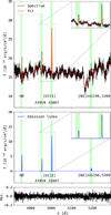Fig. 2

Spectrum from the bulge region with the fit by GANDALF. Top: flux-corrected spectrum (black), best fit by GANDALF (red), which is the sum of the model stellar and the emission line spectra. The green shaded areas are the regions where the emission lines are expected. A zoom into the region of the [O III] doublet is shown on the right. Middle: best fit emission lines with a zoom into the region of the [O III] doublet. Bottom: residuals (f_measured − f_fitted)/f_measured.

Close examination of the spectra showed that in many regions multiple gascomponents at different radial velocities exist. In order to properly treat these multiple peaks, we added another [O III] component to be fitted with GANDALF, as well as a second Hβ component and a second [N I] component. The initial guesses for the gas velocities have to be slightly different for the two components, otherwise GANDALF does not fit separate components. An example of a fit with two lines is shown in Fig. 3. Here, the two lines have almost the same amplitude and are clearly separated.

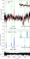Fig. 3

Spectrum from the outer edges of the bulge region where the emission lines are split into two lines with almost equal amplitudes. The plot is analogous to Fig. 2.

This was not always seen so clearly, there were also cases where one line was stronger than the other or where the two lines were almost blended together or where there was only one line clearly visible with a skewed line shape, that could, however, be described by the combination of two lines. In Fig. 4, we show where we found one line and two lines. We saw only one line in about 3000 bins, while we saw two lines in about 3500.

Fig. 4

Map of regions where the emission lines exhibit two peaks (red) and where they only have one (blue). The location of the spectrum with one peak from Fig. 2 is marked with the cyan dot, the location of the spectrum with two peaks from Fig. 3 is marked with the magenta dot.

In orderto reliably fit the different components, we had to feed GANDALF information whether only one component was present or ifthere were really two. In order to get these initial guesses, we applied the following method: First, we cross-correlated a model spectrum only consisting of the [O III]λ5007 line with each spectrum. The program fitted the resulting cross-correlation function with a set of gaussians. These gaussians all had the same dispersion of σ = 20 km s⁻¹ and their peak velocities were 40 km s⁻¹ apart. The program changed the amplitudes of the individual Gaussians to get the best approximation of the input cross-correlated spectrum. We told the program to only pick the Gaussian with the largest amplitude to have an estimate for the one-component fit and the one with the largest amplitude plus the onewith the second largest amplitude for the two component estimate. If the amplitude of the second component was less than 0.25% of the amplitude of the first one, we decided to take the initial guess with only one component. We also discarded unrealistically high velocity dispersions of σ_gas > 100 km s⁻¹. We used the central velocities of the Gaussians as the initial guesses for GANDALF, letting it fit one line for the cases where we had found only one line and letting it fit two lines where we had found two lines. After a first iteration, we checked all fits manually, updated the initial guesses for the spectra where the fit failed and let GANDALF fit a second iteration. This second iteration resulted in 85% of the spectra being fitted correctly, the rest was left out of the analysis.

In order to check if the spectra could be contaminated by a contribution of Planetary Nebulae (PNe), we looked at the catalog of PNe positions from Merrett et al. (2006). If the position of a PNe is closer than 1.6′′ (the radius of a fiber), we took this bin as affected. Overall, 166 bins were affected, which is 2.5%. All of these spectra showed [O III] lines, about two thirds of them showed two lines, while one third showed only one line. The spectra did not look systematically different from the unaffected spectra, there was for example no exceptionally bright line in any of them. We therefore concluded that contamination by PNe is negligible.

3.3 Flux calibration

In each observation night, we observed photometric standard stars, they are listed in Table B.3. These spectra were compared to photometrically calibrated spectra from the literature (Oke 1990; Le Borgne et al. 2003) to get the throughput for the particular observation night as a function of wavelength. The throughput curves were calculated with a program from Müller (2014), the error for the throughput curve is about 4%.

The atmospheric extinction was also corrected for each individual observation. Differences in observing conditions between the individual pointings were taken into account by comparing the integrated flux f_tot in one spectrum to the flux f_V of a photometric model image. This image was constructed by combining the bulge-disk decomposition by Kormendy & Bender (1999) with an ellipse fit to a K-band image performed by S10. The model image is shown in Fig. 5.

Fig. 5

Model image of M 31, constructed by combining the V -band magnitude from the decomposition of Kormendy & Bender (1999) with an ellipse fit to a K-band image by S10.

GANDALFcalculates 1-σ errors in the routine, which are consistent with what we obtained from Monte-Carlo simulations of fitting a noiseless spectrum with random added noise. These 1-σ errors are the onestabulated in Table B.7.

4 Results

4.1 Stellar kinematics

In this section, the stellar kinematics measured with GANDALF is presented. The data will be made available at the CDS, an example is given in Tables B.4 and B.5. The former table lists the individual on-sky fiber positions and the corresponding bin numbers that the fiber signals were assigned to. The latter table gives the actual stellar and gas kinematic data and the gas flux values with respectto the on-sky aperture size of the VIRUS-W fibers.

We compare our data with the measurements by S10 in the in Appendix A. In general, both datasets agree very well.

The stellar velocity map is plotted in Fig. 6, the heliocentric velocity of M 31 (v_sys = −300 km s⁻¹; de Vaucouleurs et al. 1991) has been subtracted.

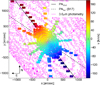Fig. 6

Map of the stellar velocity corrected for the systemic velocity of M 31. The solid straight line is the disk major axis at PA _disk = 38∘, the dashed straight line is the bar major axis at PA _bar = 55.7∘ from B17. The magenta contours are the surface brightness of the IRAC 3.6 μm image by Barmby et al. (2006). The line in the colorbar is the median errorbar of the velocities.

A schematic view of M 31 based on Henderson (1979) is plotted in Fig. 7, with the naming of the receding and approaching sides of M 31 taken from the stellar velocity map in Fig. 6. Overall, the stellar velocity field is regular, rotation is clearly visible. The velocities increase strongest along the disk major axis, with the highest velocity in the bulge region being v_{bulge, max} = 136 ± 4 km s⁻¹ in the outermost bulge pointing in the receding side and the lowest being v_{bulge, min} = −157 ± 4 km s⁻¹ on the opposite side. The “bulge region” is the region of M 31 where the bulge-to-total ratio of M 31 is higher than 0.5, taken from a decomposition by Kormendy & Bender (1999). The absolute maximum of the velocities is reached with v_max = 208 ± 3 km s⁻¹ in the outermost disk major axis disk pointing in the receding side, and the lowest value of v_min= −193 ± 2 km s⁻¹ already reached in the disk pointing at a radius of 930′′ on the approaching side. On that side, the velocity roughly remains at that value to the outermost radii. The median velocity error is d v = 3.8 km s⁻¹. When plotting the velocity map with contours, a twist for the line of zero velocity becomes apparent which not aligned with the photometric minor axis (see Fig. 8).

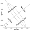Fig. 7

Schematic view of M 31. A generic ellipse with ellipticity ϵ = 0.78 is plotted, this corresponds to an inclination angle of i = 77∘ , the disk major axis has position angle PA = 38∘. The half of the galaxy to the north-west of the major axis is the near side (Henderson 1979).

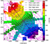Fig. 8

Map of the stellar velocity from Fig. 6 plotted with contours. The solid line is the disk major axis (38∘ ), the dash-dotted line the disk minor axis (128∘ ) and the dashed line is the bar major axis (55.7∘ ). The magenta contours are from the IRAC 3.6 μm image. In this visualization, the line of zero velocity shows a slight twist in the eastern half of the bulge.

The stellar velocity dispersion of M 31 is plotted in Fig. 9. The velocity dispersion drops faster along the disk minor axis than the major axis. The red regions are two lobes with high values of velocity dispersion of over 165 km s⁻¹, they are separated by a line of lower velocity dispersion along the major axis of the bar. Around this we see a region with slightly lower values ( ≈160 km s⁻¹) that has theshape of a small yellow parallelogram. Further out, we see a light blue region, which has even lower values of σ ( ≈130 km s⁻¹), which is elongated along the disk major axis. The maximum value is σ_max = 188 ± 5 km s⁻¹, located at a distance of 46′′ from the center, the minimum value is σ_min = 55 ± 4 km s⁻¹, in the outermost northern disk pointing at x = −100′′ and y = 1100′′. The mean velocity dispersion for the whole dataset is σ_mean = 116 ± 4 km s⁻¹, in the central 20′′ it is σ_central = 160 ± 5 km s⁻¹, considering only the bulge region it is σ_{mean, bulge} = 137 ± 4 km s⁻¹, in the disk it is considerably lower with σ_mean,disk = 103 ± 4 km s⁻¹. The disk velocity dispersion is still quite high, which is in agreement with what Fabricius et al. (2012b) find for similar disk galaxies.

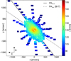Fig. 9

Stellar velocity dispersion map with the disk major axis with PA _disk = 38∘ (solid line) and the bar major axis with PA _bar = 55.7∘ (dashed line) from the model by B17.

In Fig. 10, we plot the Gauss-Hermite moment h3. In the very central 100′′, h3 has high positive and negative values, while further out, the absolute values become lower. Even further out in the bulge, the absolute values become higher again. In the disk along the major axis, the signs of h3 flip and even higher absolute values are reached. Corresponding regions of high and low values are relatively symmetric with respect to the center.

Fig. 10

Map of h3, the third moment of the Gauss-Hermite series. The lines are analogous to Fig. 9.

In the central 50′′, h3 has values of about ±0.05. Further out, the values drop to about ±0.02, before rising at the edges of the bulge region to ±0.08. In the bulge, the mean absolute value is 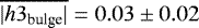$\bar{| h 3_{bulge} |} = 0.03 \pm 0.02$ $\overline{|h3_{\textrm{bulge}}|} = 0.03 \pm 0.02$ . In the disk, the values are higher, the mean absolute disk value is 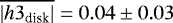$\bar{| h 3_{disk} |} = 0.04 \pm 0.03$ $\overline{|h3_{\textrm{disk}}|} = 0.04 \pm 0.03$ . Along the disk major axis, the values are highest, here, the mean absolute value is $\bar{| h 3_{major} |} = 0.07 \pm 0.02$ $\overline{|h3_{\textrm{major}}|} = 0.07 \pm 0.02$ . The maximum and minimum values of the whole map are also found along the disk major axis, being h3_max = 0.14 ± 0.02 and h3_min = −0.16 ± 0.02. Over most of the bulge region, we see a correlation between h3 and v, this will be discussed in Sect. 5.

In Fig. 11, the Gauss-Hermite moment h4 is presented. This map shows that along the disk major axis, the absolute values of h4 are very low. At the ends of the bulge region, the values of h4 become negative. Perpendicular to the disk major axis, the values of h4 become positive. The mean value over the whole dataset is $\bar{h 4} = 0.02 \pm 0.02$ $\overline{h4}=0.02 \pm 0.02$ . In a 240′′ wide and 350′′ long strip along the disk major axis, the mean value is lower, at $\bar{h 4_{outer bulge}} = 0.002$ $\overline{h4_{\textrm{outer\ bulge}}}=0.002$ . Along the disk minor axis, the values of h4 are generally higher, in regions that have a distance to the disk major axis of more than 120′′ , the mean value is $\bar{h 4_{minor}} = 0.03$ $\overline{h4_{\textrm{minor}}}=0.03$ . In the disk pointings along the disk major axis, h4 is higher in the northern half of the galaxy, having a mean value of $\bar{h 4_{major, north}} = 0.04$ $\overline{h4_{\textrm{major, north}}}=0.04$ , while in the southern half, it is $\bar{h 4_{major, south}} = - 0.01$ $\overline{h4_{\textrm{major, south}}}=-0.01$ .

Fig. 11

Map of h4, the fourth moment in the Gauss-Hermite series. The lines are analogous to Fig. 9.

4.2 Gas kinematics

In this section, the kinematics of the ionized gas is presented. These data will be made available at the CDS, an example is given in Table B.6. The motions of the gas are more complicated than the ones of the stars from Sect. 4. In the center two lobe-like regions withhigh values of velocity dispersion of over 165 km s⁻¹ can be seen.They are separated by a narrow ridge of lower velocity dispersion that is roughly aligned with the major axis. At larger radii one sees a region with slightly lower values ( ≈160 km s⁻¹) that has the shape of a parallelogram. Further out towards the edge of the bulge region, the velocity dispersion takes values of about 130 km s⁻¹. This region forms an elongated rim around the bulge region and is aligned with the disk major axis. More complicated gas kinematics are often observed in disk galaxies (e.g., Falcón-Barroso et al. 2006; Ganda et al. 2006), because contrary to the dissipationless stars, the gas can also lose energy through radiation. The dense gas traced by ground-state CO and H I transitions is most likely to have settled onto closed orbits via hydrodynamic interactions.Associated with this dense gas are regions of ionized gas (Stark & Binney 1994), which is then seen in the optical emission lines. As mentioned in Sect. 2, we observed in about half of the investigated binned spectra two gas components separated in velocity. We tried several ways to sortthe two components, either by flux or proximity in position space. In the end, we settled on sorting by velocity, because it produced the smoothest maps. The velocity map of the first component, which is the faster one of the two, is plotted in Fig. 12, the one of the second component in Fig. 13. The first gas component has a median absolute value of $\bar{| v_{[OIII], 1} |} = 162 \pm 5$ $\overline{|v_{\textrm{[OIII],1}}|}=162 \pm 5$ km s⁻¹. The maximum value is v_[OIII],1,max = 294.7 ± 4.5 km s⁻¹ at the coordinates ( − 220′′, 281′′ ), at 360′′ from the center along the disk major axis in the receding side. The minimum value is v_[OIII],1,min = −340 ± 3.0 km s⁻¹ at the coordinates (25′′, − 100′′), which is at about 100′′ south of the center in the approaching side. The minimum is closer to the center than the maximum on the other side, leading to an asymmetric appearance with respect to the center. Apart from that, there is a “spiral-like signature” in the innermost 100′′ × 100′′ and a large “S-shape” between the approaching and receding gas velocities. These structures are marked in the magnified inset of Fig. 12.

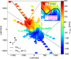Fig. 12

Velocity map of the more rapidly rotating first gas component. The lines are analogous to Fig. 9. The inset shows a zoom into the inner regions, with the S-shape highlighted along the line with systemic velocity. The spiral-like signature is highlighted with the magenta line, which encompasses both arms of the spiral. Both these structures are mentioned in the text.

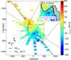Fig. 13

Velocity map of the more slowly rotating second gas component. The lines are analogous to Fig. 9. The inset shows a zoom into the inner regions, with the S-shape and the low-velocity arm highlighted, which are mentioned in the text.

Fig. 14

Velocity dispersion of the first gas component. The lines are analogous to Fig. 9.

Fig. 15

Velocity dispersion of the second gas component. The lines are analogous to Fig. 9.

For the second component, the median absolute value is significantly lower than for the first component, with $\bar{| v_{[OIII], 2} |} = 73.2 \pm 5.5$ $\overline{|v_{\textrm{[OIII],2}}|}=73.2 \pm 5.5$ km s⁻¹. The maximum value is v_[OIII],2,max = 183.8 ± 5.2 km s⁻¹ at the coordinates ( − 190′′, 280′′), which is in the same region as the maximum for the first component. The minimum value is v_[OIII],2,min = −240.2 ± 3.8 km s⁻¹, at the coordinates (65′′, − 170′′), at 182′′ from the center along the disk major axis in the receding side. This again corresponds to a region of low velocities in the first component. The overall shape of the velocity field for the second component is similar to the first, also with an S-shape along the line of zero velocity. This structure has a slightly different shape than the one for the first component, an arm of approaching velocities is extending further into the region of receding velocities. Additionally, on the western side of the bulge, at about 500′′ along the disk major axis from the center, there is an arm of velocities of about zero. This arm seems to be unconnected to the kinematics of the rest of this component. These structures are marked in the magnified inset of Fig. 13.

The velocity dispersion of the first component is plotted in Fig. 14. The general appearance is noisy, overall, the mean value is $\bar{σ_{[OIII], 1}} = 35 \pm 5$ $\overline{\sigma_{\textrm{[OIII],1}}} = 35 \pm 5$ km s⁻¹. The velocitydispersion is low near the northern end of the bulge along the major axis, where the velocities are high (σ ≈ 50−60 km s⁻¹).

In the velocity dispersion values of the second component, a ring-like structure of high values is visible, which increases the mean value of the velocity dispersion to $\bar{σ_{[OIII], 2}} = 37 \pm 6$ $\overline{\sigma_{\textrm{[OIII],2}}}=37 \pm 6$ km s⁻¹. The values in the ring are $\bar{σ_{[OIII], 2}} = 57 \pm 10$ $\overline{\sigma_{\textrm{[OIII],2}}} = 57 \pm 10$ km s⁻¹. This ring of high velocity dispersions corresponds to a similar ring in Fig. 4, which is where two peaks are measured. In this ring, a second peak with a lower amplitude than the first peak is present. However, this second peakis broader, therefore the velocity dispersion is larger.

4.3 Gas fluxes

The fluxes of Hβ, [O III]λ5007 and [N I]λ5198 are plotted in Figs. 16 to 24. The values will be made available at the CDS, an example is given in Table B.7. In Figs. 16 and 17, we show the line flux of the first and second Hβ line, while in Fig. 18, we show the sum of the two components. The corresponding fluxes for [O III]λ5007 are shown inFigs. 19–21. The plots for [N I]λ5198 are plotted in Figs. 22–24.

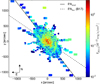Fig. 16

Flux of first Hβ component. The median error is 10⁻¹⁷ [erg s⁻¹ cm⁻²]. The lines are analogous to Fig. 9.

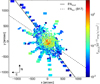Fig. 17

Flux of second Hβ component. The median error is 10⁻¹⁷ [erg s⁻¹ cm⁻²]. The lines are analogous to Fig. 9.

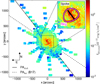Fig. 18

Flux of both Hβ components combined. The median error is 2 × 10⁻¹⁷ [erg s⁻¹ cm⁻²]. The lines are analogous to Fig. 9. The inset shows a zoom into the inner 200′′ × 200′′, with the structures ring and spoke highlighted, which are mentioned in the text.

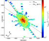Fig. 19

Flux of first [O III] component. The median error is 10⁻¹⁷ [erg s⁻¹ cm⁻²]. The lines are analogous to Fig. 9.

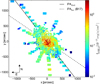Fig. 20

Flux of the second [O III] component. The median error is 10⁻¹⁷ [erg s⁻¹ cm⁻²]. The lines are analogous to Fig. 9.

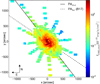Fig. 21

Sum of the flux of the two [O III] components. The median error is 2 × 10⁻¹⁷ [erg s⁻¹ cm⁻²]. The lines are analogous to Fig. 9.

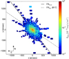Fig. 22

Flux of the first [N I] component. The median error is 10⁻¹⁷ [erg s⁻¹ cm⁻²]. The lines are analogous to Fig. 9.

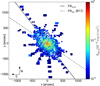Fig. 23

Flux of the second [N I] component. The median error is 10⁻¹⁷ [erg s⁻¹ cm⁻²]. The lines are analogous to Fig. 9.

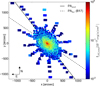Fig. 24

Total flux of the two [N I] components. The median errorbar is 10⁻¹⁷ [erg s⁻¹ cm⁻²]. The lines are analogous to Fig. 9.

There are regions where the first component has higher flux than the second one, as well as regions where the opposite is true. When averaging the fluxes along ellipses, however, it becomes apparent that the first component is stronger than the second one. This is true for all different lines. In the Hβ and [O III] maps, a spiral structure is visible over most of the bulge region, with an incomplete elliptical ring inside, which is oriented roughly along the minor axis, with a “spoke” along the ring’s short axis. The ring and spoke are highlighted in the zoomed-in inset of Fig. 18. This ring is at a smaller radius than the one mentioned above in the velocity dispersion of the second gas component. In the southwest, one of the arms of the spiral pattern is prominent in the Hβ and the [O III]. The fluxes of Hβ are lower than the ones of [O III]. The [N I] is much fainter than either the Hβ or the [O III], no clear pattern can be seen there apart from the fact that it becomes brighter in the center. The overall filamentary appearance of the gas morphology could be either due to heating by shocks or supernovae of type Ia (Jacoby et al. 1985).

We fitted ellipses to the maps of the [O III] gas and compared them to the stellar surface brightness. The comparison is shown in Fig. 25. From about 30′′ to about 200′′ , the decline of the [O III] is similar to the one of the stars, while further out, it drops significantly compared to the light of the stars. This corresponds to the edge of the spiral structure visible in the maps. The second [O III] component has lower flux values, its profile is more irregular, but it also declines fast from 200′′ outwards.

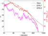Fig. 25

Comparison of the surface brightness of the stars (black) taken from Kormendy & Bender (1999) with ellipse fits to the fluxes of the first [O III] component (red) and the second [O III] component (magenta).The left y-axis is valid for the stellar surface brightness, the one on the right for the fluxes of the two gas components. The scales have been adjusted sothat the profiles for the stars and the first [O III] component can be compared easily.

5 Bar signatures in kinematics and morphology

5.1 Bar signatures in the stellar kinematics

A bar leaves certain signatures in the kinematics of the stars. Bureau & Athanassoula (2005) model several bars, with different strengths and viewing angles. Stark & Binney (1994), Athanassoula & Beaton (2006) and B17 all find that the bar in M 31 is neither viewed end-on nor side-on, but instead at an intermediate angle. The special signatures of a bar are plateaus in the velocity and the velocity dispersion, and minima in the higher moments h3 and h4. These are theoretically predicted by Bureau & Athanassoula (2005) and measured on several barred galaxies by Chung & Bureau (2004). We adopted the model of B17 as the one against which we compared our results. In their model, the bar has a position angle of PA _bar = 55.7∘, extending out to 600′′ in projection. However, in the direction of the bar, our coverage only extends to 500′′ , we are therefore missing the crucial regions of the end of the bar. Pointings covering these regions are being observed and the results will be presented in a future paper. The co-rotation radius of B17 and the outer Lindblad resonance are also outside our observed regions.

In Fig. 26, cuts through the kinematic fields along the disk major axis are plotted. Left corresponds to the north-eastern receding side, right to the south-western approaching side. The velocity rises to 70 km s⁻¹ at 35′′ , before remaining relatively constant until 350′′ on the left and 460′′ on the right, before reaching 160 km s⁻¹ at − 750′′ on the left and at 660′′ on the right. An axisymmetric stellar disk rises rapidly, but smoothly and remains flat at large radii. Bureau & Athanassoula (2005) find that a bar seen end-on produces a “double-hump” profile, where the velocity rises rapidly to a local maximum, then drops slightly to create a local minimum and then rises again slowly to the flat section at the end. When the bar is not seen end-on, but at an intermediate angle, this behavior is weakened and the local maximum and minimum disappear and form a single plateau at moderate radii, which is what we seein the profiles of M 31. This is expected from the models by B17, where the bar is seen at an intermediate angle. The rising part of the velocity curve comes from the orbits of the stars that are parallel to the bar, while the slower growth afterwards, or the local minimum inthe case of an end-on bar, is caused by an inner ring structure caused by the bar (Bureau & Athanassoula 2005).

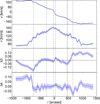Fig. 26

Cuts through the stellar kinematic maps from VIRUS-W along the disk major axis (PA = 38∘). In the third panel, the horizontal line is h3 = 0. The vertical dashed lines highlight the position where h3 has a local maximum or minimum.

The velocity dispersion profile in Fig. 26 shows that σ has two off-centered maxima, with a slight drop of about 8 km s⁻¹ in between. This drop was first observed by Kormendy (1988), who sees it as evidence for a central disk and subsequently the supermassive black hole. Bureau & Athanassoula (2005) find that such minima can also be caused by the bar, because the orbits parallel to the bar become more circular and thus lower the dispersion, however, the minimum in models by Bureau & Athanassoula (2005) is usually much stronger than what we measure here. One should keep in mind that such minima are not uniquely related to bars. Comerón et al. (2008) suggest that cold gas is accreted to the center and a subsequent starburst creates then stars with low velocity dispersion. They claim that the gas is most probably driven into the center by spiral arms, but also, albeit less probable, bars.

An inner disk can also lead to this minimum, such a structure has been found in the very center of M 31 (Tremaine 1995; Peiris & Tremaine 2003), however, with a scalelength of only about 1′′ , this structure is not resolved by our observations. The drop could also be caused by the classical bulge (B17). σ drops to 140 km s⁻¹ at 400′′ , before staying roughly constant out to 600′′ and then reaching 80 km s⁻¹ at 950′′ . These plateaus, which are not completely flat, but only less inclined than the rest of the profile, are also frequently seen in barred galaxies (Bureau & Athanassoula 2005).

The h3profile in Fig. 26 shows that the slope of h3 changes sign several times. The maxima and minima in h3 correspond to the points where the slope of the velocity profile changes, this is similar to the behavior of the simulations by Bureau & Athanassoula (2005) and has also been observed in barred galaxies (Fisher 1997; Chung & Bureau 2004; Falcón-Barroso et al. 2006; Ganda et al. 2006).

In Fig. 27, we show the correlation between h3 and v. In the outer regions, h3 is anti-correlated to v, which is theexpected behavior for disky structures in a galaxy (Binney & Tremaine 1987; Bender et al. 1994; Fisher 1997; Binney & Tremaine 2008). In the central 30′′ , h3 is again anti-correlated to the velocity. This could mean that a disky structure is also present at the center, potentially explaining the slight drop in velocity dispersion. The radial extent of this central anti-correlation corresponds roughly to the rapidly rising part of the rotation curve, a behavior that is also seen in other disk galaxies (Chung & Bureau 2004) and interpreted as a decoupled inner disk. In between the two anti-correlated regions, h3 becomes correlated with the velocity, which is taken by Bureau & Athanassoula (2005) to be a sign for a bar. The correlated region is oriented more along the bar major axis than the disk major axis. It is more prominent in the south-west than in the north, because the northern edge of the bulge is more affected by dust (Draine et al. 2014). The correlation means that there are more stars rotating faster than the circular velocity in projection, which may be a consequence of elongated motions. However, the correlation does not necessarily have to be caused by a bar, it can also be caused by the superposition of an axisymmetric bulge component embedded in a rotating disk, depending on the bulge-to-disk ratio. If the bulge is brighter than the disk, the observed mean velocity is going to be biased towards the bulge stars, with the disk creating a tail of high-velocity material (van der Marel & Franx 1993; Bureau & Athanassoula 2005).

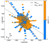Fig. 27

Correlation between the stellar velocity and h3. Plotted is sign(h3 ⋅ v), with the disk and bar major axis from Fig. 9. The color blue represents where the two quantities are anti-correlated, while in orange areas, they are correlated.

The h4 profile in Fig. 26 is relatively constant, with the exception of a minimum at 670′′ , where h4 drops from 0 to − 0.07. This minimum corresponds to the radius where h3 reaches its maximum. On the opposite side, the drop in h4 at − 750′′ is not as pronounced. Outside of 1000′′ , the values of h4 stay roughly constant at larger values of ≈0.01 for positive radii and ≈0.07 for negative radii. B/P bulges often show dips in the very center in h4 (Debattista et al. 2005; Méndez-Abreu et al. 2008), however, this only applies to low inclinations of i < 30∘. It is therefore not surprising that we do not see a central drop in h4 in M 31.

5.2 Bar signatures in the gas kinematics and morphology

The simulations of Athanassoula & Beaton (2006) and B17 do not take into account the gas content in M 31. However, the gas content in M 31 is estimated to be only ≈ 7% of the stellar mass (Corbelli et al. 2010), so we can safely assume that the gas will follow the potential set by the stellar and dark matter components. A detailed discussion of the gas behavior in this potential is provided in Blaña et al. (in prep.). As mentioned above, the velocity maps for both gas components display an S-shape in the line of zero velocity. This S-shape is stronger than the twist in the stellar velocity field. Such S-shaped twists in the gas velocity are characteristic of velocity fields with oval distortions or bars (Bosma 1981). Many barred galaxies show them, like NGC 1068 (Emsellem et al. 2006), NGC 1300 (Peterson & Huntley 1980), NGC 2683 (Kuzio de Naray et al. 2009), NGC 3386 (García-Barreto & Rosado 2001) and NGC 5448 (Fathi et al. 2005).

The region of very low velocities at the edge of the bulge on the near side of the galaxy could be produced by a large scale warp in the gas. Such a warp can project small velocities from further out into the line-of-sight (Melchior & Combes 2011).

In Figs. 28 and 29, position-velocity diagrams are plotted for the gas. We show the gas kinematics in this way to compare with similar diagrams from measurements and simulations of neutral gas, for example Chemin et al. (2009) and Athanassoula & Beaton (2006). Figure 28 shows the first component and Fig. 29 the second one. In this way, differences between the two components become immediatelyapparent. Both components occupy different regions in the PV-diagrams. The two components are real as they have different velocities. We also compared these PV-diagrams to the ones of the planetary nebulae from Merrett et al. (2006). As expected, neither gas component corresponds to the PNe, since the PNe follow the kinematics of stars.

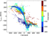Fig. 28

Position-velocity diagram of the first componentprojected onto the disk major axis at PA = 38∘, the x-axis is the distance along the major axis, the y-axis is the velocity and the color represents the perpendicular distance to the major axis. Values on the far side of the major axis are shown in blue, values on the near side in red.

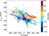Fig. 29

Position-velocity diagram of the second gas component projected onto the disk major axis. Theplot is analogous to Fig. 28. The orange and red points between 0′′ < r < 500′′ , 0 km s⁻¹ < v < 100 km ⁻¹ and 100′′ < d < 200′′ correspond to the arm of zero velocity visible in Fig. 13. To the left of the center, there is an almost flat band of negative velocities, this is the zone of approaching velocities on the eastern side of the bulge in Fig. 13.

In the PV-diagram of the first gas component, there is a prominent steep band of velocities in the center. On the receding side, the velocities stay more or less constant once they reach the plateau. The second component also shows a similar steep band of velocities as the first component, but it is less pronounced and much wider.

The position-velocity diagram of the first gas component agrees very well with the overall shape of the model of Berman (2001), who simulates a triaxial bulge in M 31: the velocity reaches a peak, then stays constant and rises to a second peak. The comparison plot of his data to cuts through our maps is shown in Fig. 30. While generally similar, our position-velocity diagrams appear slightly more asymmetric: for the approaching side of M 31, the peak is closer to the center than for the other side.

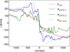Fig. 30

Cut through the velocity maps along the disk major axis within an aperture of 40′′ . The red line is a cut through the stellar velocity (Fig. 6), the blue one is a cut through the first velocitycomponent (Fig. 12), the green one the second velocity component (Fig. 13). The blackdashed line is the velocity for the triaxial bar model by Berman (2001).

The overall shape of the position-velocity diagram is very similar to what is seen in simulations (Athanassoula & Bureau 1999) and observations of barred galaxies (Bureau & Athanassoula 1999; Merrifield & Kuijken 1999), however, it could also be compatible with the superposition of other structures, like rings and disks, but this discussion goes beyond the scope of this paper.

The pattern that is visible in the flux maps in [O III] and Hβ is similar to the one seen by Jacoby et al. (1985) in a Hα + [N II] filter and in [O III], by Boulesteix et al. (1987) in [N II] and by Ciardullo et al. (1988) in Hα + [N I]. As seen in Sect. 4.3, the Hβ and [O III] maps have the overall appearance of a spiral structure, with an incomplete elliptical ring inside, which is oriented roughly along the minor axis, with a spoke along the ring’s short axis. The 100′′ long spoke along the disk major axis could be an inner disk that is projected to the observed elongated structure at M 31’s inclination (Jacoby et al. 1985). The inner spiral pattern seems to be tipped to a lower inclination with respect to the outer part, which according to Jacoby et al. (1985) can be caused by a non-axisymmetry, like a bar, and cannot be explained by axisymmetric features alone.

While the ring structure lies in the region where B17 find two inner Lindblad resonances, it is hard to deproject the structures we see in our images. A detailed analysis of the structures is postponed to a later paper, where gas will be taken into account in the dynamical model.

The fact that the incomplete ring is aligned along the minor axis, almost perpendicular to the position of the assumed bar, leads Block et al. (2006) to conclude that this ring is not caused by a bar, but by the collision of M 31 with M 32, which also caused a split of the so-called 10 kpc ring, which is a structure appearing further out in the gas. While the collision model is in better agreement with the ring structure, especially with the fact that the rings are off-centered, it has low flux inside the ring, whereas in our flux maps, as well as the ones by Jacoby et al. (1985), Boulesteix et al. (1987) and Ciardullo et al. (1988), there is flux present there. We therefore think that the bar is a more likely explanation for the rings. However, as mentioned above, to fully reproduce the visible gas rings, we need to include gas into our bar models, which will be done in the future.

5.3 Bar or triaxial bulge?

The first models that tried to explain the triaxiality in M 31 (Stark 1977; Stark & Binney 1994; Berman 2001; Berman & Loinard 2002) called their structures a “triaxial bulge” instead of a “bar”. These two concepts are fundamentally different: a bar is a rotating structure that results from an instability in the disk, while a triaxial bulge is a consequence of an anisotropy in velocity dispersion, generated, for example, by a merging processes. However, as already stated in Sect. 1, the models in the aforementioned papers actually describe rapidly rotating systems, which in our understanding are bars.

After buckling, most observed bars consist of a three-dimensional inner part of the bar, the B/P bulge, and a flat outer part (see e.g., Athanassoula 2005 or Martinez-Valpuesta et al. 2006). In this nomenclature, the triaxial bulge of the models by Berman (2001) and Berman & Loinard (2002) is a B/P bulge. Nevertheless, it is still interesting to see if our findings are also consistent with a completely non-rotating structure:

Firstly, we attempt to quantify the level of cylindrical rotation in M 31, as cylindrical rotation is generally attributed to the presence of a bar (Bureau et al. 2006). Based on Saha & Gerhard (2013), Molaeinezhad et al. (2016, hereafter M16) define the parameter m_cyl = m_avg + 1 where m_avg is a measure of the change in rotational velocity in the direction perpendicular to the major axis. m_avg averages over the slopes of the decrease in rotational velocity within the bulge region at various distances to the minor axis. M16 first test the discriminatory power of this quantity on data from the Giraffe Inner Bulge Survey (Zoccali et al. 2014) of the Milky Way and on a barred N-body model of the Milky Way by Martinez-Valpuesta & Gerhard (2011), and then apply it to 12 further disk galaxies with inclinations ranging from 70∘ to 90∘. They find that the B/P bulges in their sample as well as the Milky Way bulge show levels of cylindrical rotation of m_cyl ≃ 0.7.

As M16 we derived rotation curves parallel and at varying distances to the major axis of M 31 first and then turned these into one-sided rotation curves parallel to the minor axis at varying distances to the minor axis. We performed this analysis on the south-eastern half of M 31 as it is this half where the disk is located on the far side, such that the bulge kinematics are not affected by dust screening of the disk. For the extent of the bulge along the major axis and along the minor axis we adopted values of 460′′ and 270′′ respectively from the bulge to disk decomposition in Kormendy & Bender (1999) and used the photometric disk position angle of 38∘ (de Vaucouleurs 1958). The resulting plot is shown in Fig. 31. The parameter m_cyl for the south-eastern side is 0.72. Changing the exact values of the position angle and also varying the radii for the bulge in major axis direction and in minor axis direction, and also the area of exclusion around the major axis (we use 50′′ ) had a minor effect on m_cyl. Tests showed that for reasonable parameter ranges the value never becomes smaller than 0.68. Hence the level of cylindrical rotation – as quantified by this method – seems to be consistent to what is reported in M16 for their B/P bulges.

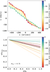Fig. 31

Measurement of the cylindrical rotation of the south-east side of M 31 according to the method by Molaeinezhad et al. (2016). Top: stellar line-of-sight velocity parallel to the major axis of galaxies at different heights from the disk plane. Bottom: line-of-sight velocity gradient parallel to the minor axis at different distances from the minor axis. Profiles are color-coded according to the distance from the minor axis. The solid black profile represents the average value m_avg . The cylindrical rotation is then m_cyl =m_avg + 1 as a quantity to express the level of cylindrical rotation.

Secondly, as described in Athanassoula & Beaton (2006) and B17, the spurs in the photometry outside the bulge argue for a planar bar, the “thin” or “long bar” component described in both papers. Although both papers give different lengths for the thin-barcomponents, the fact still remains that such a component is required to explain the photometric appearance of the galaxy.

Thirdly,the outer 10 kpc ring of M 31 is associated with the outer Lindblad resonance of the bar by B17. This structure is only possible in a rotating barred potential, as there are no characteristic resonance radii in non-rotating triaxial potentials. In a system with a triaxial bulge, this ring would be an ad-hoc feature which is difficult to explain.

Finally, the correlation between v and h3 (see Fig. 27) is a clear signature for a bar and not a triaxial bulge.

5.4 Explanations for multiple components

Several scenarios have been suggested by various authors for the origin of the multiple gas components. When gas is subject to a non-axisymmetric potential like a bar, it leads to the formation of gas streams and rings, see for example Kim et al. (2012) for numeric models. The line-of-sight passes through several of these streams, therefore leading to multiple peaks in the gas lines. A detailed comparison will only be possible once gas is included into the dynamical model, which will be done in a future paper.

There is also an alternative explanation for such streams and rings in M 31, which is that they were created by the collisionof M 31 with its small companion galaxy M 32 (Block et al. 2006). A galaxy with similar inclination as M 31, which has also a B/P bulge, is NGC 2683, which has been observed by Kuzio de Naray et al. (2009). Investigating the Hα velocity field, they see S-shaped twists and argue for the presence of a bar at a position angle of 5∘ higher than the disk position angle. Differences in their PV-diagram and the ones for M 31 lead Melchior & Combes (2011) to conclude that the interpretation of Athanassoula & Beaton (2006) in terms of a bar in M 31 is wrong and that the ring structures are only due to the collision of M 31 with M 32 suggested by Block et al. (2006). However, the bar in NGC 2683 is only at an angle of 5∘ to the disk major axis, so it is seen quite side-on, whereas the bar in M 31 is at an angle of 17∘ to the disk major axis and it is seen more end-on, which can explain the differences according to Kuzio de Naray et al. (2009).

Melchior & Combes (2011) also measure molecular emission lines in CO with two peaks, in Melchior & Combes (2016) sometimes even three. While the molecular gas is not expected to follow the ionized gas, it is still interesting that they also observe a line splitting. Melchior & Combes (2011) try to explain the double CO components with a tilted ring model coming from the collision model by Block et al. (2006). A small disk with inclination of 43∘ – more face-on than the large-scale disk of M 31 – is surrounded by a ring. The velocity profiles extracted from the simulated velocity fields by Melchior & Combes (2011) consist of a very broad component, which is blueshifted and a narrow one, which is redshifted, the blueshifted part comes from the inner disk and the redshifted part from the ring. Our [O III] measurements taken at the same positions look quite different, both components roughly have the same width, so the scenario of Melchior & Combes (2011) does not predict the actual shape of our measured [O III] spectrum.

Another scenario for multiple components is that large-scale warps in the outer galaxy disk project lower velocities from the outer regions into the inner disk. In the neutral H I gas, Chemin et al. (2009) find up to five different gas components in M 31. The velocity maps for all these components look very similar and have basically the same regular kinematic pattern. A component with a steep slope in velocity in the center is the main H I component, while components with flatter slopes are due to slower gas in the outer H I disk that is projected into the central areas due to warps in the H I disk. However Athanassoula & Beaton (2006) conclude that the different slopes can be explained by the streaming gas motions caused by the bar. Comparing the position-velocity diagrams of Chemin et al. (2009) with our own, we found that their main H I component agrees with the first gas component that we observed while the zero velocity spiral arm in the second component agrees with warped components in H I. However, it should be kept in mind that the spatial resolution in Chemin et al. (2009) in the center is lower than our own.

5.5 Ionization mechanisms of the gas

In order to investigate which mechanisms are responsible for ionizing the gas, diagnostic diagrams are used, which compare the ratios of line fluxes of different emission lines. The most widely utilized of these diagrams compares [O III]λ5007∕Hβ to [O I]λ6300∕Hα (Veilleux & Osterbrock 1987). Since Hα or [O I]λ6300 lie outside our observed wavelength range, we could not use this standard diagnostic diagram. Sarzi et al. (2010) devises alternative diagnostic diagrams for the SAURON spectrograph (Bacon et al. 2001), which has a similar wavelength range as VIRUS-W. This diagram compares [O III]λ5007∕Hβ to [N I]λλ5198, 5200∕Hβ. The [N I] lines are usually present in partially ionized regions in gaseous nebulae, which are photo-ionized by a spectrum containing high-energy photons, but they are absent in H II regions, where Hβ and [O III]λ5007 arise. The Sarzi diagram for the first [O III] component is shown in Fig. 32, the one for the second component in Fig. 33. There is not much difference between the two diagrams, the data points occupy similar regions in both.

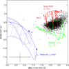Fig. 32

Diagnostic diagram for the first gas component. The plot is equivalent to the right panel of Fig. 1 in Sarzi et al. (2010). The black points are the values from our data. The median error values of the errorbars are shown in the lower left corner. Overplotted are lines showing the predictions for gas that is photoionized by a central active galactic nucleus (AGN), by O-stars after starbursts or by shocks, respectively. The AGN grids are from the dusty, radiation pressure-dominated models of Groves et al. (2004) and adopt three values for the index α of the power-law AGN continuum f_ν ∝ ν^α, with α = −1.7, − 1.4, − 1.2 from left to right. In each AGN model grid, the solid lines trace the dimensionless ionization parameter log U (defined as logq∕c), which increases with the [O III]/Hβ ratio, assuming the values logU = −3.0, − 2.6, − 2.3, − 2.0, − 1.6, − 1.3, − 1.0, whereas the dashed lines show the adopted values for the electron density of N_e = 10² and 10⁴ cm⁻³, with smaller values of the [N I]/Hβ ratio corresponding to larger N_e values. The starburst grids are from Dopita et al. (2000), and assume a gas density of N_e = 350 cm⁻³ and use a spectral energy distribution obtained from models from Starburst99 (Leitherer et al. 1999) for an instantaneous star formation episode. The grids assume a range of metallicity Z for both stars and gas in the starburst, shown by the solid lines for Z = 0.2, 0.4, 1.0, 2.0 Z_⊙, and different values for the ionization parameter q, shown by the dashed lines for q = 0.5, 1, 2, 4, 8, 15, 30 × 10⁷ cm s⁻¹. The shock grids, without precursor H II region, are from Allen et al. (2008) and assume an electron density of N_e = 1 cm⁻³ and a solar value for the gas metallicity. The solid lines show models with increasing shock velocity v = 150, 200, 300, 500, 750, 1000 km s⁻¹, and the dashed lines models with magnetic parameter b = 0.5, 1.0, 2.0, 4.0. The grids were obtained using the program ITERA (Groves & Allen 2010). We assumed solar metallicity for the shocks and twice solar metallicity for the dusty active galactic nucleus (AGN) grids, because we measured these values in the bulge in our stellar population measurements, which will be presented in Saglia et al. (2018).

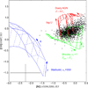Fig. 33

Diagnostic diagram for the second component. The plot is equivalent to Fig. 32, with the grids being the same.

The ionization does not happen via starbursts, instead most of the points lie in the region where the ionization is due to shocks in the gas. That shocks are the primary source for ionization issupported by the fact that the emission seems to be strengthened along the lines of the velocity discontinuities. These shocks could be triggered by the bar. About half the points, however, also lie in between the Shock region and the AGN region, which is occupied by Seyfert galaxies in Sarzi et al. (2010), but since the AGN in M 31 is very weak (del Burgo et al. 2000), excitation by the AGN is unlikely. These datapoints lying between the regions can be partially explained by the fact that the errors of the datapoints are large. Furthermore, the diagnostic diagram used here does not present as clear separations as the usual [O I]/Hα vs. [O III]/Hβ diagram, compare Sarzi et al. (2006). Contamination by planetary nebulae is also not an issue, we checked the 166 bins that are affected by PNe. They lie in the upper parts of the shock grid and between the shock and the AGN grid, there is no systematic offset of the PNe positions with respect to the rest of our spectra.

6 Conclusions

6.1 Main results

For several decades, the question has been posed if M 31 is a barred galaxy or not (Lindblad 1956; Stark 1977; Stark & Binney 1994; Athanassoula & Beaton 2006; B17). The high inclination of M 31 made it difficult for a long time to see the bar directly in optical photometry. Twists in the inner isophotes were the first hints for its existence (Lindblad 1956; Stark 1977), while more recently, the boxy appearance of the isophotes in infrared images was used to constrain its orientation and length (Beaton et al. 2007; B17). However, a kinematic confirmation of the bar has been missing so far.

In this paper, we have presented results from observations of M 31 with the optical integral field unit spectrograph VIRUS-W. We derived the kinematic properties of the stars and two different ionized gas components and measure the gas fluxes. We found hints in the kinematics that M 31 contains a bar. Our main results are:

1.
Cuts through the stellar velocity field reveal a plateau at moderate radii, which is a signature that can be created by a bar that is seen at an intermediate angle (Bureau & Athanassoula 2005). The line of zero velocity does not coincide with the photometric minor axis and shows a twist toward the edge of the bulge.
2.
The stellar velocity dispersion field shows a drop in the center, with two maxima aligned along the minor axis. While this central drop can be caused by inner disky structures or dust in the center (Falcón-Barroso et al. 2006) or the classical bulge (B17), it can also be due to the bar, since the stellar orbits that make up the bar become more circular in the center (Bureau & Athanassoula 2005). There are also two inclined plateaus at intermediate radii in the σ profile, a behavior that is also often seen in barred potentials (Bureau & Athanassoula 2005).
3.
The Gauss-Hermite moment h3 is anti-correlated with the velocity v in the disk regions and the very center, which is the expected behavior for a disk component (Bender et al. 1994). In the majority of the bulge region, h3 is correlated with the velocity v, which can be achieved by elongated motions which occur along the bar direction (Bureau & Athanassoula 2005).
4.
The gas kinematics, measured using the [O III]λ5007 line, is more complicated than the stellar kinematics. Many spectra exhibit two separate peaks, resulting in two kinematically distinct components. One of the two components has faster velocities than the other one. The fast component has disk-like rotation with a very steep gradient in the center. The line of zero velocity is S-shaped, again pointing to a bar. The overall shape of the rotation curve of the first component is qualitatively in agreement with gas in a barred dynamical model of M 31 by Berman (2001).
5.
The position-velocity diagrams of the gas components look similar to what is expected from simulations (Athanassoula & Beaton 2006), with arms of steep and flatter slopes. The overall shape of the position-velocity diagram agrees with observations in H I by Chemin et al. (2009). They measure up to 5 different components, the most luminous of which is the main H I disk, which coincides with the steep slope in the position-velocity diagram. The other components belong to the branches with lower slope in the position-velocity diagrams. According to Chemin et al. (2009), they are low velocities from the outer regions of the H I disk, which have been projected to the center due to warps. However, they can also agree with the lower velocity branches that exist in a barred potential (Athanassoula & Beaton 2006).
6.
When looking at the morphology of the gas, we see a spiral pattern, similar to what is described by Jacoby et al. (1985) in Hα + [N II] and [O III], Boulesteix et al. (1987) in [N II] and Ciardullo et al. (1988) in Hα + [N II]. This spiral pattern has a lower inclination than the disk, which means it could have been tilted by a non-axisymmetry, like a bar (Jacoby et al. 1985).
7.
Block et al. (2006) find that the morphology of M 31 in the far infrared is not caused by a bar, but is instead the result of a density wave caused by the collision of M 32 with M 31. Comparing their gas morphology with our measured one, the ring somewhat corresponds to what we see, but there is no high emission inside the ring, which we observe in [O III]. Building on this model, Melchior & Combes (2011) propose a scenario of a tilted ring in the center over another rotating disk, to explain line splittings they measure in CO observations. Their model predicts that the component in the ring has a very narrow line, while the disk leads to a very broad line, which is not what wesee, our two components in that region have the same width. We therefore think that this model is inconsistent with our observations.
8.
From diagnostic diagrams for the ionization of the gas, we find that the gas is mostly ionized by shocks and not by starbursts, which is consistent with the low star formation rate of M 31 (Davidge et al. 2012). This is also in agreement by the filamentary appearance of the gas morphology, which could be either due to shocks or supernovae of type Ia (Jacoby et al. 1985).

To summarize, there are several hints in the kinematics of the stars and the ionized gas and its morphology for a bar in M 31.

6.2 Future work

From the analysis of the absorption line strengths, we measured the age, metallicity and α/Fe-overabundance of the stellar populations. These results will be presented in an accompanying paper (Saglia et al. 2018). These measurements, combined with the kinematics presented in this paper, are used as a basis for a made-to-measure dynamical model (Blaña et al., in prep.). This model will allow us to truly test the bar hypothesis and to check if our observations are caused by the bar, especially once gas is taken into account. They will also provide new estimates on the number of microlensing events caused by MACHOs or self-lensing, which will be used in future microlensing surveys toward M 31. We also plan to observe further pointings along the bar major axis, to calculate the pattern speed of the bar.

Appendix A A Comparison with data from S10

We compared the stellar and gas kinematics measured with VIRUS-W with the ones from S10. S10 observed M 31 with a longslit spectrograph along 6 directions, the slit positions are plotted in Fig. A.1. We generated cuts through our own stellar velocity maps along the slit directions of S10 and compared them with their data in Fig. A.2. Our velocities agree within 5% with the ones by S10, except for the minor axis on the near side (positive radii in Fig. A.2), where the deviation is about 30%. The comparison plot for the velocity dispersion is shown in Fig. A.3. Overall, our data agree well with the measurements of S10, but we do not reproduce the central spike in σ that is caused by the supermassive black hole, because we lack resolution in the very central regions. The overall agreement is within 4%. The comparison for h3 can be seen in Fig. A.4. The standard deviation of the difference between our values and the ones by S10 is 0.020–0.027, which agrees with the root mean square value of the error of the VIRUS-W values.

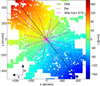Fig. A.1

Velocity map with disk major axis (PA = 38∘, solid black line), the bar major axis (PA = 55.7∘, dashed black line) and the slit positions by S10 (magenta). They are PA = 48∘ (the bulge major axis), PA = 78∘, PA = 108∘, PA = 138∘ (the bulge minor axis), PA = 108∘ and PA= 18∘, all angles measured east from north. The line in the colorbar is the median errorbar of the velocities.

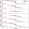Fig. A.2

Comparison of our velocities with the ones from S10. Black are the velocities measured by S10, red are cuts through our velocity maps along the same directions.

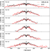Fig. A.3

Comparison of our velocity dispersions with the ones from S10. Black are the values measured by S10, red are cuts through our velocity dispersion maps along the same directions.

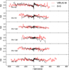Fig. A.4

Comparison of the measured h3 values with the ones from S10. Black are the values measured by S10, red are cuts through our maps along the same directions.

In Fig. A.5, the corresponding cuts for h4 are shown. Again, we find good agreement, the standard deviation of the difference between our values and the ones by S10 is 0.02, which agrees with the root mean square of the error of the VIRUS-W values.

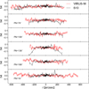Fig. A.5

Comparison of the measured h4 values with the ones from S10. Black are the values measured byS10, red are cuts through maps along the same directions.

We also compared our gas kinematics to the data from S10. The comparison plot is shown in Fig. A.6. Generally, the first component agrees with the values from S10. For large radii, the velocity from S10 often lies between both velocity components. This is expected, the spectral resolution in S10 ( ≈69 km s⁻¹) does not resolve the two gas components, so consequently they observe a single broader line at intermediate velocity. Similarly, the single component gas velocity dispersions of S10 are affected by the relatively lower spectral resolution and tend to be systematically larger than our values. Still, overall our data agree very well with S10.

Fig. A.6

Comparison of our gas velocities with the ones from S10. Black are the velocities measured by S10, red are cuts through the first gas component from Fig. 12 and blue the cuts through the second component from Fig. 13.

Appendix B Observed objects and lines for wavelength calibration

Table B.1

Lines used for wavelength calibration.

Table B.2

Kinematic standard stars.

Table B.3

Photometric standard stars.

Table B.4

Bin information.

Table B.5

Kinematic data of the stars.

Table B.6

Kinematic data of the gas.

Table B.7

Photometric data of the gas.

References

Adams, J. J., Blanc, G. A., Hill, G. J., et al. 2011, ApJS, 192, 5 [NASA ADS] [CrossRef] [Google Scholar]
Afonso, C., Albert, J. N., Andersen, J., et al. 2003, A&A, 400, 951 [NASA ADS] [CrossRef] [EDP Sciences] [Google Scholar]
Alcock, C., Akerlof, C. W., Allsman, R. A., et al. 1993, Nature, 365, 621 [NASA ADS] [CrossRef] [Google Scholar]
Alcock, C., Allsman, R. A., Alves, D. R., et al. 2000, ApJ, 542, 281 [NASA ADS] [CrossRef] [Google Scholar]
Allen, M. G., Groves, B. A., Dopita, M. A., Sutherland, R. S., & Kewley, L. J. 2008, ApJS, 178, 20 [Google Scholar]
Athanassoula, E. 2005, MNRAS, 358, 1477 [NASA ADS] [CrossRef] [Google Scholar]
Athanassoula, E., & Beaton, R. L. 2006, MNRAS, 370, 1499 [NASA ADS] [CrossRef] [Google Scholar]
Athanassoula, E., & Bureau, M. 1999, ApJ, 522, 699 [NASA ADS] [CrossRef] [Google Scholar]
Athanassoula, E., & Misiriotis, A. 2002, MNRAS, 330, 35 [NASA ADS] [CrossRef] [Google Scholar]
Aubourg, E., Bareyre, P., Bréhin, S., et al. 1993, Nature, 365, 623 [NASA ADS] [CrossRef] [Google Scholar]
Bacon, R., Copin, Y., Monnet, G., et al. 2001, MNRAS, 326, 23 [NASA ADS] [CrossRef] [Google Scholar]
Barazza, F. D., Jogee, S., & Marinova, I. 2008, ApJ, 675, 1194 [NASA ADS] [CrossRef] [Google Scholar]
Barmby, P., Ashby, M. L. N., Bianchi, L., et al. 2006, ApJ, 650, L45 [NASA ADS] [CrossRef] [Google Scholar]
Beaton, R. L., Majewski, S. R., Guhathakurta, P., et al. 2007, ApJ, 658, L91 [NASA ADS] [CrossRef] [Google Scholar]
Bender, R., Saglia, R. P., & Gerhard, O. E. 1994, MNRAS, 269, 785 [NASA ADS] [CrossRef] [Google Scholar]
Berman, S. 2001, A&A, 371, 476 [NASA ADS] [CrossRef] [EDP Sciences] [Google Scholar]
Berman, S., & Loinard, L. 2002, MNRAS, 336, 477 [NASA ADS] [CrossRef] [Google Scholar]
Bertone, G. 2010, Particle Dark Matter: Observations, Models and Searches (Cambridge University Press) [CrossRef] [Google Scholar]
Binney, J., & Tremaine, S. 1987, Galactic Dynamics (Princeton: Princeton University Press) [Google Scholar]
Binney, J., & Tremaine, S. 2008, Galactic Dynamics: Second Edition (Princeton University Press) [Google Scholar]
Blaña Díaz, M., Wegg, C., Gerhard, O., et al. 2017, MNRAS, 466, 4279 [NASA ADS] [Google Scholar]
Block, D. L., Bournaud, F., Combes, F., et al. 2006, Nature, 443, 832 [NASA ADS] [CrossRef] [Google Scholar]
Bosma, A. 1981, AJ, 86, 1825 [NASA ADS] [CrossRef] [Google Scholar]
Boulesteix, J., Georgelin, Y. P., Lecoarer, E., Marcelin, M., & Monnet, G. 1987, A&A, 178, 91 [NASA ADS] [Google Scholar]
Brinks, E., & Burton, W. B. 1984, A&A, 141, 195 [NASA ADS] [Google Scholar]
Brinks, E., & Shane, W. W. 1984, A&AS, 55, 179 [NASA ADS] [Google Scholar]
Bureau, M., & Athanassoula, E. 1999, ApJ, 522, 686 [NASA ADS] [CrossRef] [Google Scholar]
Bureau, M., & Athanassoula, E. 2005, ApJ, 626, 159 [NASA ADS] [CrossRef] [Google Scholar]
Bureau, M., Aronica, G., Athanassoula, E., et al. 2006, MNRAS, 370, 753 [NASA ADS] [CrossRef] [Google Scholar]
Cappellari, M., & Copin, Y. 2003, MNRAS, 342, 345 [NASA ADS] [CrossRef] [Google Scholar]
Cappellari, M., & Emsellem, E. 2004, PASP, 116, 138 [NASA ADS] [CrossRef] [Google Scholar]
Chemin, L., Carignan, C., & Foster, T. 2009, ApJ, 705, 1395 [NASA ADS] [CrossRef] [Google Scholar]
Chung, A., & Bureau, M. 2004, AJ, 127, 3192 [NASA ADS] [CrossRef] [Google Scholar]
Ciardullo, R., Rubin, V. C., Ford, Jr., W. K., Jacoby, G. H., & Ford, H. C. 1988, AJ, 95, 438 [NASA ADS] [CrossRef] [Google Scholar]
Combes, F., & Sanders, R. H. 1981, A&A, 96, 164 [NASA ADS] [Google Scholar]
Combes, F., Debbasch, F., Friedli, D., & Pfenniger, D. 1990, A&A, 233, 82 [NASA ADS] [Google Scholar]
Comerón, S., Knapen, J. H., & Beckman, J. E. 2008, A&A, 485, 695 [NASA ADS] [CrossRef] [EDP Sciences] [Google Scholar]
Corbelli, E., Lorenzoni, S., Walterbos, R., Braun, R., & Thilker, D. 2010, A&A, 511, A89 [NASA ADS] [CrossRef] [EDP Sciences] [Google Scholar]
Courteau, S., Widrow, L. M., McDonald, M., et al. 2011, ApJ, 739, 20 [NASA ADS] [CrossRef] [Google Scholar]
Dalcanton, J. J., Williams, B. F., Lang, D., et al. 2012, ApJS, 200, 18 [NASA ADS] [CrossRef] [Google Scholar]
Davidge, T. J., McConnachie, A. W., Fardal, M. A., et al. 2012, ApJ, 751, 74 [NASA ADS] [CrossRef] [Google Scholar]
de Grijs, R., & Bono, G. 2014, AJ, 148, 17 endrefcommentnewpage [NASA ADS] [CrossRef] [Google Scholar]
de Vaucouleurs G. 1958, ApJ, 128, 465 [NASA ADS] [CrossRef] [Google Scholar]
de Vaucouleurs, G., de Vaucouleurs, A., Corwin, Jr., H. G., et al. 1991, Third Reference Catalogue of Bright Galaxies. Volume I: Explanations and references. Volume II: Data for galaxies between 0^h and 12^h. Volume III: Data for galaxies between 12^h and 24^h. [Google Scholar]
Debattista, V. P., Carollo, C. M., Mayer, L., & Moore, B. 2005, ApJ, 628, 678 [NASA ADS] [CrossRef] [Google Scholar]
del Burgo, C., Mediavilla, E., & Arribas, S. 2000, ApJ, 540, 741 [NASA ADS] [CrossRef] [Google Scholar]
Dopita, M. A., Kewley, L. J., Heisler, C. A., & Sutherland, R. S. 2000, ApJ, 542, 224 [NASA ADS] [CrossRef] [Google Scholar]
Draine, B. T., Aniano, G., Krause, O., et al. 2014, ApJ, 780, 172 [NASA ADS] [CrossRef] [Google Scholar]
Emsellem, E., Fathi, K., Wozniak, H., et al. 2006, MNRAS, 365, 367 [NASA ADS] [CrossRef] [Google Scholar]
Erwin, P., & Debattista, V. P. 2016, ApJ, 825, L30 [NASA ADS] [CrossRef] [Google Scholar]
Eskridge, P. B., Frogel, J. A., Pogge, R. W., et al. 2000, AJ, 119, 536 [NASA ADS] [CrossRef] [Google Scholar]
Fabricius, M. H., Coccato, L., Bender, R., et al. 2014, MNRAS, 441, 2212 [NASA ADS] [CrossRef] [Google Scholar]
Fabricius, M. H., Grupp, F., Bender, R., et al. 2012a, in SPIE Conf. Ser. 8446 [Google Scholar]
Fabricius, M. H., Saglia, R. P., Fisher, D. B., et al. 2012b, ApJ, 754, 67 [NASA ADS] [CrossRef] [Google Scholar]
Falcón-Barroso, J., Bacon, R., Bureau, M., et al. 2006, MNRAS, 369, 529 [NASA ADS] [CrossRef] [Google Scholar]
Fathi, K., van de Ven, G., Peletier, R. F., et al. 2005, MNRAS, 364, 773 [NASA ADS] [CrossRef] [Google Scholar]
Fisher, D. 1997, AJ, 113, 950 [NASA ADS] [CrossRef] [Google Scholar]
Fritz, J., Gentile, G., Smith, M. W. L., et al. 2012, A&A, 546, A34 [NASA ADS] [CrossRef] [EDP Sciences] [Google Scholar]
Ganda, K., Falcón-Barroso, J., Peletier, R. F., et al. 2006, MNRAS, 367, 46 [NASA ADS] [CrossRef] [Google Scholar]
García-Barreto, J. A., & Rosado, M. 2001, AJ, 121, 2540 [NASA ADS] [CrossRef] [Google Scholar]
Gerhard, O. E. 1993, MNRAS, 265, 213 [NASA ADS] [CrossRef] [Google Scholar]
Gerhard, O. E., & Wegg, C. 2015, in Lessons from the Local Group – A Conference in honour of David Block and Bruce Elmegreen, ed. K. Freeman, B. Elmegreen, D. Block, & M. Woolway (Berlin, Heidelberg, New York: Springer-Verlag) [Google Scholar]
Gilbert, K. M., Guhathakurta, P., Kalirai, J. S., et al. 2006, ApJ, 652, 1188 [NASA ADS] [CrossRef] [Google Scholar]
Gilbert, K. M., Guhathakurta, P., Kollipara, P., et al. 2009, ApJ, 705, 1275 [NASA ADS] [CrossRef] [Google Scholar]
Gilbert, K. M., Guhathakurta, P., Beaton, R. L., et al. 2012, ApJ, 760, 76 [NASA ADS] [CrossRef] [Google Scholar]
Gilbert, K. M., Kalirai, J. S., Guhathakurta, P., et al. 2014, ApJ, 796, 76 [NASA ADS] [CrossRef] [Google Scholar]
Gordon, K. D., Bailin, J., Engelbracht, C. W., et al. 2006, ApJ, 638, L87 [Google Scholar]
Gössl, C. A.,& Riffeser, A. 2002, A&A, 381, 1095 [NASA ADS] [CrossRef] [EDP Sciences] [Google Scholar]
Griest, K. 1991, ApJ, 366, 412 [NASA ADS] [CrossRef] [Google Scholar]
Groves, B. A., & Allen, M. G. 2010, New Astron., 15, 614 [NASA ADS] [CrossRef] [Google Scholar]
Groves, B. A., Dopita, M. A., & Sutherland, R. S. 2004, ApJS, 153, 75 [NASA ADS] [CrossRef] [Google Scholar]
Guhathakurta, P., Ostheimer, J. C., Gilbert, K. M., et al. 2005, ArXiv e-prints [arXiv:astro-ph/0502366] [Google Scholar]
Guhathakurta, P., Rich, R. M., Reitzel, D. B., et al. 2006, AJ, 131, 2497 [NASA ADS] [CrossRef] [Google Scholar]
Hamadache, C., Le Guillou, L., Tisserand, P., et al. 2006, A&A, 454, 185 [NASA ADS] [CrossRef] [EDP Sciences] [Google Scholar]
Henderson, A. P. 1979, A&A, 75, 311 [NASA ADS] [Google Scholar]
Hernández-López, I., Athanassoula, E., Mújica, R., & Bosma, A. 2009, in Rev. Mex. Astron. Astrofis. Conf. Ser. 37, 160 [Google Scholar]
Hill, G. J., Gebhardt, K., Komatsu, E., & MacQueen, P. J. 2004, in Amer. Inst. Phys. Conf. Ser. 743, The New Cosmology: Conference on Strings and Cosmology, ed. R. E. Allen, D. V. Nanopoulos, & C. N. Pope, 224 [Google Scholar]
Ibata, R. A., Lewis, G. F., Conn, A. R., et al. 2013, Nature, 493, 62 [CrossRef] [Google Scholar]
Jacoby, G. H., Ford, H., & Ciardullo, R. 1985, ApJ, 290, 136 [NASA ADS] [CrossRef] [Google Scholar]
Kim, W.-T., Seo, W.-Y., Stone, J. M., Yoon, D., & Teuben, P. J. 2012, ApJ, 747, 60 [NASA ADS] [CrossRef] [Google Scholar]
Kirk, J. M., Gear, W. K., Fritz, J., et al. 2015, ApJ, 798, 58 [NASA ADS] [CrossRef] [Google Scholar]
Kormendy, J. 1988, ApJ, 325, 128 [NASA ADS] [CrossRef] [Google Scholar]
Kormendy, J., & Bender, R. 1999, ApJ, 522, 772 [NASA ADS] [CrossRef] [Google Scholar]
Kormendy, J., Fisher, D. B., Cornell, M. E., & Bender, R. 2009, ApJS, 182, 216 [NASA ADS] [CrossRef] [Google Scholar]
Kormendy, J., Drory, N., Bender, R., & Cornell, M. E. 2010, ApJ, 723, 54 [NASA ADS] [CrossRef] [Google Scholar]
Kuzio de Naray, R., Zagursky, M. J., & McGaugh, S. S. 2009, AJ, 138, 1082 [NASA ADS] [CrossRef] [Google Scholar]
Le Borgne, J.-F., Bruzual, G., Pelló, R., et al. 2003, A&A, 402, 433 [NASA ADS] [CrossRef] [EDP Sciences] [Google Scholar]
Lee, C.-H., Riffeser, A., Koppenhoefer, J., et al. 2012, AJ, 143, 89 [NASA ADS] [CrossRef] [Google Scholar]
Lee, C.-H., Koppenhoefer, J., Seitz, S., et al. 2014a, ApJ, 797, 22 [NASA ADS] [CrossRef] [Google Scholar]
Lee, C.-H., Seitz, S., Kodric, M., et al. 2014b, ApJ, 785, 11 [NASA ADS] [CrossRef] [Google Scholar]
Lee, C.-H., Riffeser, A., Seitz, S., Bender, R., & Koppenhoefer, J. 2015, ApJ, 806, 161 [NASA ADS] [CrossRef] [Google Scholar]
Leitherer, C., Schaerer, D., Goldader, J. D., et al. 1999, ApJS, 123, 3 [NASA ADS] [CrossRef] [Google Scholar]
Lindblad, B. 1956, Stockholms Observatoriums Annaler, 19 [Google Scholar]
Martinez-Valpuesta, I., & Gerhard, O. 2011, ApJ, 734, L20 [NASA ADS] [CrossRef] [Google Scholar]
Martinez-Valpuesta, I., Shlosman, I., & Heller, C. 2006, ApJ, 637, 214 [NASA ADS] [CrossRef] [Google Scholar]
McConnachie, A. W., Irwin, M. J., Ibata, R. A., et al. 2009, Nature, 461, 66 [NASA ADS] [CrossRef] [PubMed] [Google Scholar]
Meeks, M. L. 1976, Methods of experimental physics Vol. 12. Astrophysics Part C: Radio observations [Google Scholar]
Melchior, A.-L., & Combes, F. 2011, A&A, 536, A52 [NASA ADS] [CrossRef] [EDP Sciences] [Google Scholar]
Melchior, A.-L., & Combes, F. 2016, A&A, 585, A44 [NASA ADS] [CrossRef] [EDP Sciences] [Google Scholar]
Méndez-Abreu, J., Corsini, E. M., Debattista, V. P., et al. 2008, ApJ, 679, L73 [NASA ADS] [CrossRef] [Google Scholar]
Menéndez-Delmestre, K., Sheth, K., Schinnerer, E., Jarrett, T. H., & Scoville, N. Z. 2007, ApJ, 657, 790 [NASA ADS] [CrossRef] [Google Scholar]
Merrett, H. R., Merrifield, M. R., Douglas, N. G., et al. 2006, MNRAS, 369, 120 endrefcommentnewpage [NASA ADS] [CrossRef] [Google Scholar]
Merrifield, M. R., & Kuijken, K. 1999, A&A, 345, L47 [NASA ADS] [Google Scholar]
Merritt, D., & Sellwood, J. A. 1994, ApJ, 425, 551 [NASA ADS] [CrossRef] [Google Scholar]
Molaeinezhad, A., Falcón-Barroso, J., Martínez-Valpuesta, I., et al. 2016, MNRAS, 456, 692 [NASA ADS] [CrossRef] [Google Scholar]
Müller, F. 2014, Development of a Fiber Based Integral Field Unit and Derivation of the Instrumental Response Function of an Existing Integral Field Unit [Google Scholar]
Oke, J. B. 1990, AJ, 99, 1621 [NASA ADS] [CrossRef] [Google Scholar]
Paczynski, B. 1986, ApJ, 304, 1 [NASA ADS] [CrossRef] [Google Scholar]
Peiris, H. V., & Tremaine, S. 2003, ApJ, 599, 237 [NASA ADS] [CrossRef] [Google Scholar]
Peterson, C. J., & Huntley, J. M. 1980, ApJ, 242, 913 [NASA ADS] [CrossRef] [Google Scholar]
Planck Collaboration XVI 2014, A&A, 571, A16 [NASA ADS] [CrossRef] [EDP Sciences] [Google Scholar]
Planck Collaboration XIII 2016, A&A, 594, A13 [NASA ADS] [CrossRef] [EDP Sciences] [Google Scholar]
Prugniel, P., Soubiran, C., Koleva, M., & Le Borgne D. 2007, VizieR Online Data Catalog: III/251 [Google Scholar]
Raha, N., Sellwood, J. A., James, R. A., & Kahn, F. D. 1991, Nature, 352, 411 [NASA ADS] [CrossRef] [Google Scholar]
Riffeser, A., Fliri, J., Seitz, S., & Bender, R. 2006, ApJS, 163, 225 [NASA ADS] [CrossRef] [Google Scholar]
Rubin, V. C., & Ford, Jr., W. K. 1970, ApJ, 159, 379 [NASA ADS] [CrossRef] [Google Scholar]
Rubin, V. C., & Ford, Jr., W. K. 1971, ApJ, 170, 25 [NASA ADS] [CrossRef] [Google Scholar]
Saglia, R. P., Fabricius, M., Bender, R., et al. 2010, A&A, 509, A61 [NASA ADS] [CrossRef] [EDP Sciences] [Google Scholar]
Saglia, R. P., Opitsch, M., Fabricius, M. H., et al. 2018, A&A, submitted [Google Scholar]
Saha, K., & Gerhard, O. 2013, MNRAS, 430, 2039 [NASA ADS] [CrossRef] [Google Scholar]
Sarzi, M., Falcón-Barroso, J., Davies, R. L., et al. 2006, MNRAS, 366, 1151 [NASA ADS] [CrossRef] [Google Scholar]
Sarzi, M., Shields, J. C., Schawinski, K., et al. 2010, MNRAS, 402, 2187 endrefcommentnewpage [NASA ADS] [CrossRef] [Google Scholar]
Sellwood, J. A. 2013, in Planets, Stars and Stellar Systems 5, Galactic Structure and Stellar Populations, ed. T. D. Oswalt & G. Gilmore (Berlin, Heidelberg, New York: Springer-Verlag) [Google Scholar]
Sellwood, J. A., & Wilkinson, A. 1993, Rep. Progr. Phys., 56, 173 [Google Scholar]
Smith, M. W. L., Eales, S. A., Gomez, H. L., et al. 2012, ApJ, 756, 40 [NASA ADS] [CrossRef] [Google Scholar]
Stark, A. A. 1977, ApJ, 213, 368 [NASA ADS] [CrossRef] [Google Scholar]
Stark, A. A., & Binney, J. 1994, ApJ, 426, L31 [NASA ADS] [CrossRef] [Google Scholar]
Sumi, T., Bennett, D. P., Bond, I. A., et al. 2013, ApJ, 778, 150 [NASA ADS] [CrossRef] [Google Scholar]
Tisserand, P., Le Guillou, L., Afonso, C., et al. 2007, A&A, 469, 387 [NASA ADS] [CrossRef] [EDP Sciences] [Google Scholar]
Tremaine, S. 1995, AJ, 110, 628 [NASA ADS] [CrossRef] [Google Scholar]
Udalski, A., Szymanski, M., Kaluzny, J., Kubiak, M., & Mateo, M. 1992, Acta Astron., 42, 253 [NASA ADS] [Google Scholar]
van der Marel, R. P., & Franx, M. 1993, ApJ, 407, 525 [NASA ADS] [CrossRef] [Google Scholar]
van Leeuwen F. 2007, A&A, 474, 653 [NASA ADS] [CrossRef] [EDP Sciences] [Google Scholar]
Veilleux, S., & Osterbrock, D. E. 1987, ApJS, 63, 295 [NASA ADS] [CrossRef] [Google Scholar]
Walterbos, R. A. M., & Kennicutt, Jr., R. C. 1987, A&AS, 69, 311 [NASA ADS] [Google Scholar]
Wegg, C., Gerhard, O., & Portail, M. 2016, MNRAS, 463, 557 [NASA ADS] [CrossRef] [Google Scholar]
Wenger, M., Ochsenbein, F., Egret, D., et al. 2000, A&AS, 143, 9 [NASA ADS] [CrossRef] [EDP Sciences] [Google Scholar]
Widrow, L. M., Perrett, K. M., & Suyu, S. H. 2003, ApJ, 588, 311 [NASA ADS] [CrossRef] [Google Scholar]
Williams, B. F., Lang, D., Dalcanton, J. J., et al. 2014, ApJS, 215, 9 [NASA ADS] [CrossRef] [Google Scholar]
Worthey, G., Faber, S. M., Gonzalez, J. J., & Burstein, D. 1994, ApJS, 94, 687 [NASA ADS] [CrossRef] [Google Scholar]
Wyrzykowski, Ł., Rynkiewicz, A. E., Skowron, J., et al. 2015, ApJS, 216, 12 [NASA ADS] [CrossRef] [Google Scholar]
Wyrzykowski, L., Skowron, J., Kozłowski, S., et al. 2011, MNRAS, 416, 2949 [NASA ADS] [CrossRef] [EDP Sciences] [Google Scholar]
Zoccali, M., Gonzalez, O. A., Vasquez, S., et al. 2014, A&A, 562, A66 [NASA ADS] [CrossRef] [EDP Sciences] [Google Scholar]

¹

The image has been taken from http://archive.stsci.edu/cgi-bin/dss_form. The digitized sky surveys were produced at the Space Telescope Science Institute under U.S. Government grant NAG W-2166. The images of these surveys are based on photographic data obtained using the Oschin Schmidt Telescope on Palomar Mountain and the UK Schmidt Telescope. The plates were processed into the present compressed digital form with the permission of these institutions. ©1995 by the Association of Universities for Research in Astronomy, Inc.

²

https://www.astro.virginia.edu/emm8x/utils/vlsr.html

All Tables

Table B.1

Lines used for wavelength calibration.

In the text

Table B.2

Kinematic standard stars.

In the text

Table B.3

Photometric standard stars.

Bin information.

Kinematic data of the stars.

In the text

Table B.6

Kinematic data of the gas.

In the text

Table B.7

Photometric data of the gas.

In the text

All Figures

	Fig. 1 Observed pointings of M 31 overlaid on a digitized sky survey (DSS)¹ V -band image.
In the text

Fig. 2

Spectrum from the bulge region with the fit by GANDALF. Top: flux-corrected spectrum (black), best fit by GANDALF (red), which is the sum of the model stellar and the emission line spectra. The green shaded areas are the regions where the emission lines are expected. A zoom into the region of the [O III] doublet is shown on the right. Middle: best fit emission lines with a zoom into the region of the [O III] doublet. Bottom: residuals (f_measured − f_fitted)/f_measured.

In the text

	Fig. 3 Spectrum from the outer edges of the bulge region where the emission lines are split into two lines with almost equal amplitudes. The plot is analogous to Fig. 2.
In the text

	Fig. 4 Map of regions where the emission lines exhibit two peaks (red) and where they only have one (blue). The location of the spectrum with one peak from Fig. 2 is marked with the cyan dot, the location of the spectrum with two peaks from Fig. 3 is marked with the magenta dot.
In the text

	Fig. 5 Model image of M 31, constructed by combining the V -band magnitude from the decomposition of Kormendy & Bender (1999) with an ellipse fit to a K-band image by S10.
In the text

	Fig. 6 Map of the stellar velocity corrected for the systemic velocity of M 31. The solid straight line is the disk major axis at PA _disk = 38∘, the dashed straight line is the bar major axis at PA _bar = 55.7∘ from B17. The magenta contours are the surface brightness of the IRAC 3.6 μm image by Barmby et al. (2006). The line in the colorbar is the median errorbar of the velocities.
In the text

	Fig. 7 Schematic view of M 31. A generic ellipse with ellipticity ϵ = 0.78 is plotted, this corresponds to an inclination angle of i = 77∘ , the disk major axis has position angle PA = 38∘. The half of the galaxy to the north-west of the major axis is the near side (Henderson 1979).
In the text

	Fig. 8 Map of the stellar velocity from Fig. 6 plotted with contours. The solid line is the disk major axis (38∘ ), the dash-dotted line the disk minor axis (128∘ ) and the dashed line is the bar major axis (55.7∘ ). The magenta contours are from the IRAC 3.6 μm image. In this visualization, the line of zero velocity shows a slight twist in the eastern half of the bulge.
In the text

	Fig. 9 Stellar velocity dispersion map with the disk major axis with PA _disk = 38∘ (solid line) and the bar major axis with PA _bar = 55.7∘ (dashed line) from the model by B17.
In the text

	Fig. 10 Map of h3, the third moment of the Gauss-Hermite series. The lines are analogous to Fig. 9.
In the text

	Fig. 11 Map of h4, the fourth moment in the Gauss-Hermite series. The lines are analogous to Fig. 9.
In the text

	Fig. 12 Velocity map of the more rapidly rotating first gas component. The lines are analogous to Fig. 9. The inset shows a zoom into the inner regions, with the S-shape highlighted along the line with systemic velocity. The spiral-like signature is highlighted with the magenta line, which encompasses both arms of the spiral. Both these structures are mentioned in the text.
In the text

	Fig. 13 Velocity map of the more slowly rotating second gas component. The lines are analogous to Fig. 9. The inset shows a zoom into the inner regions, with the S-shape and the low-velocity arm highlighted, which are mentioned in the text.
In the text

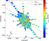	Fig. 14 Velocity dispersion of the first gas component. The lines are analogous to Fig. 9.
In the text

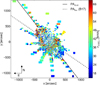	Fig. 15 Velocity dispersion of the second gas component. The lines are analogous to Fig. 9.
In the text

	Fig. 16 Flux of first Hβ component. The median error is 10⁻¹⁷ [erg s⁻¹ cm⁻²]. The lines are analogous to Fig. 9.
In the text

	Fig. 17 Flux of second Hβ component. The median error is 10⁻¹⁷ [erg s⁻¹ cm⁻²]. The lines are analogous to Fig. 9.
In the text

	Fig. 18 Flux of both Hβ components combined. The median error is 2 × 10⁻¹⁷ [erg s⁻¹ cm⁻²]. The lines are analogous to Fig. 9. The inset shows a zoom into the inner 200′′ × 200′′, with the structures ring and spoke highlighted, which are mentioned in the text.
In the text

	Fig. 19 Flux of first [O III] component. The median error is 10⁻¹⁷ [erg s⁻¹ cm⁻²]. The lines are analogous to Fig. 9.
In the text

	Fig. 20 Flux of the second [O III] component. The median error is 10⁻¹⁷ [erg s⁻¹ cm⁻²]. The lines are analogous to Fig. 9.
In the text

	Fig. 21 Sum of the flux of the two [O III] components. The median error is 2 × 10⁻¹⁷ [erg s⁻¹ cm⁻²]. The lines are analogous to Fig. 9.
In the text

	Fig. 22 Flux of the first [N I] component. The median error is 10⁻¹⁷ [erg s⁻¹ cm⁻²]. The lines are analogous to Fig. 9.
In the text

	Fig. 23 Flux of the second [N I] component. The median error is 10⁻¹⁷ [erg s⁻¹ cm⁻²]. The lines are analogous to Fig. 9.
In the text

	Fig. 24 Total flux of the two [N I] components. The median errorbar is 10⁻¹⁷ [erg s⁻¹ cm⁻²]. The lines are analogous to Fig. 9.
In the text

Fig. 25

Comparison of the surface brightness of the stars (black) taken from Kormendy & Bender (1999) with ellipse fits to the fluxes of the first [O III] component (red) and the second [O III] component (magenta).The left y-axis is valid for the stellar surface brightness, the one on the right for the fluxes of the two gas components. The scales have been adjusted sothat the profiles for the stars and the first [O III] component can be compared easily.

In the text

	Fig. 26 Cuts through the stellar kinematic maps from VIRUS-W along the disk major axis (PA = 38∘). In the third panel, the horizontal line is h3 = 0. The vertical dashed lines highlight the position where h3 has a local maximum or minimum.
In the text

	Fig. 27 Correlation between the stellar velocity and h3. Plotted is sign(h3 ⋅ v), with the disk and bar major axis from Fig. 9. The color blue represents where the two quantities are anti-correlated, while in orange areas, they are correlated.
In the text

	Fig. 28 Position-velocity diagram of the first componentprojected onto the disk major axis at PA = 38∘, the x-axis is the distance along the major axis, the y-axis is the velocity and the color represents the perpendicular distance to the major axis. Values on the far side of the major axis are shown in blue, values on the near side in red.
In the text

Fig. 29

Position-velocity diagram of the second gas component projected onto the disk major axis. Theplot is analogous to Fig. 28. The orange and red points between 0′′ < r < 500′′ , 0 km s⁻¹ < v < 100 km ⁻¹ and 100′′ < d < 200′′ correspond to the arm of zero velocity visible in Fig. 13. To the left of the center, there is an almost flat band of negative velocities, this is the zone of approaching velocities on the eastern side of the bulge in Fig. 13.

In the text

	Fig. 30 Cut through the velocity maps along the disk major axis within an aperture of 40′′ . The red line is a cut through the stellar velocity (Fig. 6), the blue one is a cut through the first velocitycomponent (Fig. 12), the green one the second velocity component (Fig. 13). The blackdashed line is the velocity for the triaxial bar model by Berman (2001).
In the text

Fig. 31

Measurement of the cylindrical rotation of the south-east side of M 31 according to the method by Molaeinezhad et al. (2016). Top: stellar line-of-sight velocity parallel to the major axis of galaxies at different heights from the disk plane. Bottom: line-of-sight velocity gradient parallel to the minor axis at different distances from the minor axis. Profiles are color-coded according to the distance from the minor axis. The solid black profile represents the average value m_avg . The cylindrical rotation is then m_cyl =m_avg + 1 as a quantity to express the level of cylindrical rotation.

In the text

Fig. 32

Diagnostic diagram for the first gas component. The plot is equivalent to the right panel of Fig. 1 in Sarzi et al. (2010). The black points are the values from our data. The median error values of the errorbars are shown in the lower left corner. Overplotted are lines showing the predictions for gas that is photoionized by a central active galactic nucleus (AGN), by O-stars after starbursts or by shocks, respectively. The AGN grids are from the dusty, radiation pressure-dominated models of Groves et al. (2004) and adopt three values for the index α of the power-law AGN continuum f_ν ∝ ν^α, with α = −1.7, − 1.4, − 1.2 from left to right. In each AGN model grid, the solid lines trace the dimensionless ionization parameter log U (defined as logq∕c), which increases with the [O III]/Hβ ratio, assuming the values logU = −3.0, − 2.6, − 2.3, − 2.0, − 1.6, − 1.3, − 1.0, whereas the dashed lines show the adopted values for the electron density of N_e = 10² and 10⁴ cm⁻³, with smaller values of the [N I]/Hβ ratio corresponding to larger N_e values. The starburst grids are from Dopita et al. (2000), and assume a gas density of N_e = 350 cm⁻³ and use a spectral energy distribution obtained from models from Starburst99 (Leitherer et al. 1999) for an instantaneous star formation episode. The grids assume a range of metallicity Z for both stars and gas in the starburst, shown by the solid lines for Z = 0.2, 0.4, 1.0, 2.0 Z_⊙, and different values for the ionization parameter q, shown by the dashed lines for q = 0.5, 1, 2, 4, 8, 15, 30 × 10⁷ cm s⁻¹. The shock grids, without precursor H II region, are from Allen et al. (2008) and assume an electron density of N_e = 1 cm⁻³ and a solar value for the gas metallicity. The solid lines show models with increasing shock velocity v = 150, 200, 300, 500, 750, 1000 km s⁻¹, and the dashed lines models with magnetic parameter b = 0.5, 1.0, 2.0, 4.0. The grids were obtained using the program ITERA (Groves & Allen 2010). We assumed solar metallicity for the shocks and twice solar metallicity for the dusty active galactic nucleus (AGN) grids, because we measured these values in the bulge in our stellar population measurements, which will be presented in Saglia et al. (2018).

In the text

	Fig. 33 Diagnostic diagram for the second component. The plot is equivalent to Fig. 32, with the grids being the same.
In the text

Fig. A.1

Velocity map with disk major axis (PA = 38∘, solid black line), the bar major axis (PA = 55.7∘, dashed black line) and the slit positions by S10 (magenta). They are PA = 48∘ (the bulge major axis), PA = 78∘, PA = 108∘, PA = 138∘ (the bulge minor axis), PA = 108∘ and PA= 18∘, all angles measured east from north. The line in the colorbar is the median errorbar of the velocities.

In the text

	Fig. A.2 Comparison of our velocities with the ones from S10. Black are the velocities measured by S10, red are cuts through our velocity maps along the same directions.
In the text

	Fig. A.3 Comparison of our velocity dispersions with the ones from S10. Black are the values measured by S10, red are cuts through our velocity dispersion maps along the same directions.
In the text

	Fig. A.4 Comparison of the measured h3 values with the ones from S10. Black are the values measured by S10, red are cuts through our maps along the same directions.
In the text

	Fig. A.5 Comparison of the measured h4 values with the ones from S10. Black are the values measured byS10, red are cuts through maps along the same directions.
In the text

	Fig. A.6 Comparison of our gas velocities with the ones from S10. Black are the velocities measured by S10, red are cuts through the first gas component from Fig. 12 and blue the cuts through the second component from Fig. 13.
In the text

Current usage metrics show cumulative count of Article Views (full-text article views including HTML views, PDF and ePub downloads, according to the available data) and Abstracts Views on Vision4Press platform.

Data correspond to usage on the plateform after 2015. The current usage metrics is available 48-96 hours after online publication and is updated daily on week days.

Initial download of the metrics may take a while.

[1] Adams, J. J., Blanc, G. A., Hill, G. J., et al. 2011, ApJS, 192, 5 [NASA ADS] [CrossRef] [Google Scholar]

[2] Afonso, C., Albert, J. N., Andersen, J., et al. 2003, A&A, 400, 951 [NASA ADS] [CrossRef] [EDP Sciences] [Google Scholar]

[3] Alcock, C., Akerlof, C. W., Allsman, R. A., et al. 1993, Nature, 365, 621 [NASA ADS] [CrossRef] [Google Scholar]

[4] Alcock, C., Allsman, R. A., Alves, D. R., et al. 2000, ApJ, 542, 281 [NASA ADS] [CrossRef] [Google Scholar]

[5] Allen, M. G., Groves, B. A., Dopita, M. A., Sutherland, R. S., & Kewley, L. J. 2008, ApJS, 178, 20 [Google Scholar]

[6] Athanassoula, E. 2005, MNRAS, 358, 1477 [NASA ADS] [CrossRef] [Google Scholar]

[7] Athanassoula, E., & Beaton, R. L. 2006, MNRAS, 370, 1499 [NASA ADS] [CrossRef] [Google Scholar]

[8] Athanassoula, E., & Bureau, M. 1999, ApJ, 522, 699 [NASA ADS] [CrossRef] [Google Scholar]

[9] Athanassoula, E., & Misiriotis, A. 2002, MNRAS, 330, 35 [NASA ADS] [CrossRef] [Google Scholar]

[10] Aubourg, E., Bareyre, P., Bréhin, S., et al. 1993, Nature, 365, 623 [NASA ADS] [CrossRef] [Google Scholar]

[11] Bacon, R., Copin, Y., Monnet, G., et al. 2001, MNRAS, 326, 23 [NASA ADS] [CrossRef] [Google Scholar]

[12] Barazza, F. D., Jogee, S., & Marinova, I. 2008, ApJ, 675, 1194 [NASA ADS] [CrossRef] [Google Scholar]

[13] Barmby, P., Ashby, M. L. N., Bianchi, L., et al. 2006, ApJ, 650, L45 [NASA ADS] [CrossRef] [Google Scholar]

[14] Beaton, R. L., Majewski, S. R., Guhathakurta, P., et al. 2007, ApJ, 658, L91 [NASA ADS] [CrossRef] [Google Scholar]

[15] Bender, R., Saglia, R. P., & Gerhard, O. E. 1994, MNRAS, 269, 785 [NASA ADS] [CrossRef] [Google Scholar]

[16] Berman, S. 2001, A&A, 371, 476 [NASA ADS] [CrossRef] [EDP Sciences] [Google Scholar]

[17] Berman, S., & Loinard, L. 2002, MNRAS, 336, 477 [NASA ADS] [CrossRef] [Google Scholar]

[18] Bertone, G. 2010, Particle Dark Matter: Observations, Models and Searches (Cambridge University Press) [CrossRef] [Google Scholar]

[19] Binney, J., & Tremaine, S. 1987, Galactic Dynamics (Princeton: Princeton University Press) [Google Scholar]

[20] Binney, J., & Tremaine, S. 2008, Galactic Dynamics: Second Edition (Princeton University Press) [Google Scholar]

[21] Blaña Díaz, M., Wegg, C., Gerhard, O., et al. 2017, MNRAS, 466, 4279 [NASA ADS] [Google Scholar]

[22] Block, D. L., Bournaud, F., Combes, F., et al. 2006, Nature, 443, 832 [NASA ADS] [CrossRef] [Google Scholar]

[23] Bosma, A. 1981, AJ, 86, 1825 [NASA ADS] [CrossRef] [Google Scholar]

[24] Boulesteix, J., Georgelin, Y. P., Lecoarer, E., Marcelin, M., & Monnet, G. 1987, A&A, 178, 91 [NASA ADS] [Google Scholar]

[25] Brinks, E., & Burton, W. B. 1984, A&A, 141, 195 [NASA ADS] [Google Scholar]

[26] Brinks, E., & Shane, W. W. 1984, A&AS, 55, 179 [NASA ADS] [Google Scholar]

[27] Bureau, M., & Athanassoula, E. 1999, ApJ, 522, 686 [NASA ADS] [CrossRef] [Google Scholar]

[28] Bureau, M., & Athanassoula, E. 2005, ApJ, 626, 159 [NASA ADS] [CrossRef] [Google Scholar]

[29] Bureau, M., Aronica, G., Athanassoula, E., et al. 2006, MNRAS, 370, 753 [NASA ADS] [CrossRef] [Google Scholar]

[30] Cappellari, M., & Copin, Y. 2003, MNRAS, 342, 345 [NASA ADS] [CrossRef] [Google Scholar]

[31] Cappellari, M., & Emsellem, E. 2004, PASP, 116, 138 [NASA ADS] [CrossRef] [Google Scholar]

[32] Chemin, L., Carignan, C., & Foster, T. 2009, ApJ, 705, 1395 [NASA ADS] [CrossRef] [Google Scholar]

[33] Chung, A., & Bureau, M. 2004, AJ, 127, 3192 [NASA ADS] [CrossRef] [Google Scholar]

[34] Ciardullo, R., Rubin, V. C., Ford, Jr., W. K., Jacoby, G. H., & Ford, H. C. 1988, AJ, 95, 438 [NASA ADS] [CrossRef] [Google Scholar]

[35] Combes, F., & Sanders, R. H. 1981, A&A, 96, 164 [NASA ADS] [Google Scholar]

[36] Combes, F., Debbasch, F., Friedli, D., & Pfenniger, D. 1990, A&A, 233, 82 [NASA ADS] [Google Scholar]

[37] Comerón, S., Knapen, J. H., & Beckman, J. E. 2008, A&A, 485, 695 [NASA ADS] [CrossRef] [EDP Sciences] [Google Scholar]

[38] Corbelli, E., Lorenzoni, S., Walterbos, R., Braun, R., & Thilker, D. 2010, A&A, 511, A89 [NASA ADS] [CrossRef] [EDP Sciences] [Google Scholar]

[39] Courteau, S., Widrow, L. M., McDonald, M., et al. 2011, ApJ, 739, 20 [NASA ADS] [CrossRef] [Google Scholar]

[40] Dalcanton, J. J., Williams, B. F., Lang, D., et al. 2012, ApJS, 200, 18 [NASA ADS] [CrossRef] [Google Scholar]

[41] Davidge, T. J., McConnachie, A. W., Fardal, M. A., et al. 2012, ApJ, 751, 74 [NASA ADS] [CrossRef] [Google Scholar]

[42] de Grijs, R., & Bono, G. 2014, AJ, 148, 17 endrefcommentnewpage [NASA ADS] [CrossRef] [Google Scholar]

[43] de Vaucouleurs G. 1958, ApJ, 128, 465 [NASA ADS] [CrossRef] [Google Scholar]

[44] de Vaucouleurs, G., de Vaucouleurs, A., Corwin, Jr., H. G., et al. 1991, Third Reference Catalogue of Bright Galaxies. Volume I: Explanations and references. Volume II: Data for galaxies between 0^h and 12^h. Volume III: Data for galaxies between 12^h and 24^h. [Google Scholar]

[45] Debattista, V. P., Carollo, C. M., Mayer, L., & Moore, B. 2005, ApJ, 628, 678 [NASA ADS] [CrossRef] [Google Scholar]

[46] del Burgo, C., Mediavilla, E., & Arribas, S. 2000, ApJ, 540, 741 [NASA ADS] [CrossRef] [Google Scholar]

[47] Dopita, M. A., Kewley, L. J., Heisler, C. A., & Sutherland, R. S. 2000, ApJ, 542, 224 [NASA ADS] [CrossRef] [Google Scholar]

[48] Draine, B. T., Aniano, G., Krause, O., et al. 2014, ApJ, 780, 172 [NASA ADS] [CrossRef] [Google Scholar]

[49] Emsellem, E., Fathi, K., Wozniak, H., et al. 2006, MNRAS, 365, 367 [NASA ADS] [CrossRef] [Google Scholar]

[50] Erwin, P., & Debattista, V. P. 2016, ApJ, 825, L30 [NASA ADS] [CrossRef] [Google Scholar]

[51] Eskridge, P. B., Frogel, J. A., Pogge, R. W., et al. 2000, AJ, 119, 536 [NASA ADS] [CrossRef] [Google Scholar]

[52] Fabricius, M. H., Coccato, L., Bender, R., et al. 2014, MNRAS, 441, 2212 [NASA ADS] [CrossRef] [Google Scholar]

[53] Fabricius, M. H., Grupp, F., Bender, R., et al. 2012a, in SPIE Conf. Ser. 8446 [Google Scholar]

[54] Fabricius, M. H., Saglia, R. P., Fisher, D. B., et al. 2012b, ApJ, 754, 67 [NASA ADS] [CrossRef] [Google Scholar]

[55] Falcón-Barroso, J., Bacon, R., Bureau, M., et al. 2006, MNRAS, 369, 529 [NASA ADS] [CrossRef] [Google Scholar]

[56] Fathi, K., van de Ven, G., Peletier, R. F., et al. 2005, MNRAS, 364, 773 [NASA ADS] [CrossRef] [Google Scholar]

[57] Fisher, D. 1997, AJ, 113, 950 [NASA ADS] [CrossRef] [Google Scholar]

[58] Fritz, J., Gentile, G., Smith, M. W. L., et al. 2012, A&A, 546, A34 [NASA ADS] [CrossRef] [EDP Sciences] [Google Scholar]

[59] Ganda, K., Falcón-Barroso, J., Peletier, R. F., et al. 2006, MNRAS, 367, 46 [NASA ADS] [CrossRef] [Google Scholar]

[60] García-Barreto, J. A., & Rosado, M. 2001, AJ, 121, 2540 [NASA ADS] [CrossRef] [Google Scholar]

[61] Gerhard, O. E. 1993, MNRAS, 265, 213 [NASA ADS] [CrossRef] [Google Scholar]

[62] Gerhard, O. E., & Wegg, C. 2015, in Lessons from the Local Group – A Conference in honour of David Block and Bruce Elmegreen, ed. K. Freeman, B. Elmegreen, D. Block, & M. Woolway (Berlin, Heidelberg, New York: Springer-Verlag) [Google Scholar]

[63] Gilbert, K. M., Guhathakurta, P., Kalirai, J. S., et al. 2006, ApJ, 652, 1188 [NASA ADS] [CrossRef] [Google Scholar]

[64] Gilbert, K. M., Guhathakurta, P., Kollipara, P., et al. 2009, ApJ, 705, 1275 [NASA ADS] [CrossRef] [Google Scholar]

[65] Gilbert, K. M., Guhathakurta, P., Beaton, R. L., et al. 2012, ApJ, 760, 76 [NASA ADS] [CrossRef] [Google Scholar]

[66] Gilbert, K. M., Kalirai, J. S., Guhathakurta, P., et al. 2014, ApJ, 796, 76 [NASA ADS] [CrossRef] [Google Scholar]

[67] Gordon, K. D., Bailin, J., Engelbracht, C. W., et al. 2006, ApJ, 638, L87 [Google Scholar]

[68] Gössl, C. A.,& Riffeser, A. 2002, A&A, 381, 1095 [NASA ADS] [CrossRef] [EDP Sciences] [Google Scholar]

[69] Griest, K. 1991, ApJ, 366, 412 [NASA ADS] [CrossRef] [Google Scholar]

[70] Groves, B. A., & Allen, M. G. 2010, New Astron., 15, 614 [NASA ADS] [CrossRef] [Google Scholar]

[71] Groves, B. A., Dopita, M. A., & Sutherland, R. S. 2004, ApJS, 153, 75 [NASA ADS] [CrossRef] [Google Scholar]

[72] Guhathakurta, P., Ostheimer, J. C., Gilbert, K. M., et al. 2005, ArXiv e-prints [arXiv:astro-ph/0502366] [Google Scholar]

[73] Guhathakurta, P., Rich, R. M., Reitzel, D. B., et al. 2006, AJ, 131, 2497 [NASA ADS] [CrossRef] [Google Scholar]

[74] Hamadache, C., Le Guillou, L., Tisserand, P., et al. 2006, A&A, 454, 185 [NASA ADS] [CrossRef] [EDP Sciences] [Google Scholar]

[75] Henderson, A. P. 1979, A&A, 75, 311 [NASA ADS] [Google Scholar]

[76] Hernández-López, I., Athanassoula, E., Mújica, R., & Bosma, A. 2009, in Rev. Mex. Astron. Astrofis. Conf. Ser. 37, 160 [Google Scholar]

[77] Hill, G. J., Gebhardt, K., Komatsu, E., & MacQueen, P. J. 2004, in Amer. Inst. Phys. Conf. Ser. 743, The New Cosmology: Conference on Strings and Cosmology, ed. R. E. Allen, D. V. Nanopoulos, & C. N. Pope, 224 [Google Scholar]

[78] Ibata, R. A., Lewis, G. F., Conn, A. R., et al. 2013, Nature, 493, 62 [CrossRef] [Google Scholar]

[79] Jacoby, G. H., Ford, H., & Ciardullo, R. 1985, ApJ, 290, 136 [NASA ADS] [CrossRef] [Google Scholar]

[80] Kim, W.-T., Seo, W.-Y., Stone, J. M., Yoon, D., & Teuben, P. J. 2012, ApJ, 747, 60 [NASA ADS] [CrossRef] [Google Scholar]

[81] Kirk, J. M., Gear, W. K., Fritz, J., et al. 2015, ApJ, 798, 58 [NASA ADS] [CrossRef] [Google Scholar]

[82] Kormendy, J. 1988, ApJ, 325, 128 [NASA ADS] [CrossRef] [Google Scholar]

[83] Kormendy, J., & Bender, R. 1999, ApJ, 522, 772 [NASA ADS] [CrossRef] [Google Scholar]

[84] Kormendy, J., Fisher, D. B., Cornell, M. E., & Bender, R. 2009, ApJS, 182, 216 [NASA ADS] [CrossRef] [Google Scholar]

[85] Kormendy, J., Drory, N., Bender, R., & Cornell, M. E. 2010, ApJ, 723, 54 [NASA ADS] [CrossRef] [Google Scholar]

[86] Kuzio de Naray, R., Zagursky, M. J., & McGaugh, S. S. 2009, AJ, 138, 1082 [NASA ADS] [CrossRef] [Google Scholar]

[87] Le Borgne, J.-F., Bruzual, G., Pelló, R., et al. 2003, A&A, 402, 433 [NASA ADS] [CrossRef] [EDP Sciences] [Google Scholar]

[88] Lee, C.-H., Riffeser, A., Koppenhoefer, J., et al. 2012, AJ, 143, 89 [NASA ADS] [CrossRef] [Google Scholar]

[89] Lee, C.-H., Koppenhoefer, J., Seitz, S., et al. 2014a, ApJ, 797, 22 [NASA ADS] [CrossRef] [Google Scholar]

[90] Lee, C.-H., Seitz, S., Kodric, M., et al. 2014b, ApJ, 785, 11 [NASA ADS] [CrossRef] [Google Scholar]

[91] Lee, C.-H., Riffeser, A., Seitz, S., Bender, R., & Koppenhoefer, J. 2015, ApJ, 806, 161 [NASA ADS] [CrossRef] [Google Scholar]

[92] Leitherer, C., Schaerer, D., Goldader, J. D., et al. 1999, ApJS, 123, 3 [NASA ADS] [CrossRef] [Google Scholar]

[93] Lindblad, B. 1956, Stockholms Observatoriums Annaler, 19 [Google Scholar]

[94] Martinez-Valpuesta, I., & Gerhard, O. 2011, ApJ, 734, L20 [NASA ADS] [CrossRef] [Google Scholar]

[95] Martinez-Valpuesta, I., Shlosman, I., & Heller, C. 2006, ApJ, 637, 214 [NASA ADS] [CrossRef] [Google Scholar]

[96] McConnachie, A. W., Irwin, M. J., Ibata, R. A., et al. 2009, Nature, 461, 66 [NASA ADS] [CrossRef] [PubMed] [Google Scholar]

[97] Meeks, M. L. 1976, Methods of experimental physics Vol. 12. Astrophysics Part C: Radio observations [Google Scholar]

[98] Melchior, A.-L., & Combes, F. 2011, A&A, 536, A52 [NASA ADS] [CrossRef] [EDP Sciences] [Google Scholar]

[99] Melchior, A.-L., & Combes, F. 2016, A&A, 585, A44 [NASA ADS] [CrossRef] [EDP Sciences] [Google Scholar]

[100] Méndez-Abreu, J., Corsini, E. M., Debattista, V. P., et al. 2008, ApJ, 679, L73 [NASA ADS] [CrossRef] [Google Scholar]

[101] Menéndez-Delmestre, K., Sheth, K., Schinnerer, E., Jarrett, T. H., & Scoville, N. Z. 2007, ApJ, 657, 790 [NASA ADS] [CrossRef] [Google Scholar]

[102] Merrett, H. R., Merrifield, M. R., Douglas, N. G., et al. 2006, MNRAS, 369, 120 endrefcommentnewpage [NASA ADS] [CrossRef] [Google Scholar]

[103] Merrifield, M. R., & Kuijken, K. 1999, A&A, 345, L47 [NASA ADS] [Google Scholar]

[104] Merritt, D., & Sellwood, J. A. 1994, ApJ, 425, 551 [NASA ADS] [CrossRef] [Google Scholar]

[105] Molaeinezhad, A., Falcón-Barroso, J., Martínez-Valpuesta, I., et al. 2016, MNRAS, 456, 692 [NASA ADS] [CrossRef] [Google Scholar]

[106] Müller, F. 2014, Development of a Fiber Based Integral Field Unit and Derivation of the Instrumental Response Function of an Existing Integral Field Unit [Google Scholar]

[107] Oke, J. B. 1990, AJ, 99, 1621 [NASA ADS] [CrossRef] [Google Scholar]

[108] Paczynski, B. 1986, ApJ, 304, 1 [NASA ADS] [CrossRef] [Google Scholar]

[109] Peiris, H. V., & Tremaine, S. 2003, ApJ, 599, 237 [NASA ADS] [CrossRef] [Google Scholar]

[110] Peterson, C. J., & Huntley, J. M. 1980, ApJ, 242, 913 [NASA ADS] [CrossRef] [Google Scholar]

[111] Planck Collaboration XVI 2014, A&A, 571, A16 [NASA ADS] [CrossRef] [EDP Sciences] [Google Scholar]

[112] Planck Collaboration XIII 2016, A&A, 594, A13 [NASA ADS] [CrossRef] [EDP Sciences] [Google Scholar]

[113] Prugniel, P., Soubiran, C., Koleva, M., & Le Borgne D. 2007, VizieR Online Data Catalog: III/251 [Google Scholar]

[114] Raha, N., Sellwood, J. A., James, R. A., & Kahn, F. D. 1991, Nature, 352, 411 [NASA ADS] [CrossRef] [Google Scholar]

[115] Riffeser, A., Fliri, J., Seitz, S., & Bender, R. 2006, ApJS, 163, 225 [NASA ADS] [CrossRef] [Google Scholar]

[116] Rubin, V. C., & Ford, Jr., W. K. 1970, ApJ, 159, 379 [NASA ADS] [CrossRef] [Google Scholar]

[117] Rubin, V. C., & Ford, Jr., W. K. 1971, ApJ, 170, 25 [NASA ADS] [CrossRef] [Google Scholar]

[118] Saglia, R. P., Fabricius, M., Bender, R., et al. 2010, A&A, 509, A61 [NASA ADS] [CrossRef] [EDP Sciences] [Google Scholar]

[119] Saglia, R. P., Opitsch, M., Fabricius, M. H., et al. 2018, A&A, submitted [Google Scholar]

[120] Saha, K., & Gerhard, O. 2013, MNRAS, 430, 2039 [NASA ADS] [CrossRef] [Google Scholar]

[121] Sarzi, M., Falcón-Barroso, J., Davies, R. L., et al. 2006, MNRAS, 366, 1151 [NASA ADS] [CrossRef] [Google Scholar]

[122] Sarzi, M., Shields, J. C., Schawinski, K., et al. 2010, MNRAS, 402, 2187 endrefcommentnewpage [NASA ADS] [CrossRef] [Google Scholar]

[123] Sellwood, J. A. 2013, in Planets, Stars and Stellar Systems 5, Galactic Structure and Stellar Populations, ed. T. D. Oswalt & G. Gilmore (Berlin, Heidelberg, New York: Springer-Verlag) [Google Scholar]

[124] Sellwood, J. A., & Wilkinson, A. 1993, Rep. Progr. Phys., 56, 173 [Google Scholar]

[125] Smith, M. W. L., Eales, S. A., Gomez, H. L., et al. 2012, ApJ, 756, 40 [NASA ADS] [CrossRef] [Google Scholar]

[126] Stark, A. A. 1977, ApJ, 213, 368 [NASA ADS] [CrossRef] [Google Scholar]

[127] Stark, A. A., & Binney, J. 1994, ApJ, 426, L31 [NASA ADS] [CrossRef] [Google Scholar]

[128] Sumi, T., Bennett, D. P., Bond, I. A., et al. 2013, ApJ, 778, 150 [NASA ADS] [CrossRef] [Google Scholar]

[129] Tisserand, P., Le Guillou, L., Afonso, C., et al. 2007, A&A, 469, 387 [NASA ADS] [CrossRef] [EDP Sciences] [Google Scholar]

[130] Tremaine, S. 1995, AJ, 110, 628 [NASA ADS] [CrossRef] [Google Scholar]

[131] Udalski, A., Szymanski, M., Kaluzny, J., Kubiak, M., & Mateo, M. 1992, Acta Astron., 42, 253 [NASA ADS] [Google Scholar]

[132] van der Marel, R. P., & Franx, M. 1993, ApJ, 407, 525 [NASA ADS] [CrossRef] [Google Scholar]

[133] van Leeuwen F. 2007, A&A, 474, 653 [NASA ADS] [CrossRef] [EDP Sciences] [Google Scholar]

[134] Veilleux, S., & Osterbrock, D. E. 1987, ApJS, 63, 295 [NASA ADS] [CrossRef] [Google Scholar]

[135] Walterbos, R. A. M., & Kennicutt, Jr., R. C. 1987, A&AS, 69, 311 [NASA ADS] [Google Scholar]

[136] Wegg, C., Gerhard, O., & Portail, M. 2016, MNRAS, 463, 557 [NASA ADS] [CrossRef] [Google Scholar]

[137] Wenger, M., Ochsenbein, F., Egret, D., et al. 2000, A&AS, 143, 9 [NASA ADS] [CrossRef] [EDP Sciences] [Google Scholar]

[138] Widrow, L. M., Perrett, K. M., & Suyu, S. H. 2003, ApJ, 588, 311 [NASA ADS] [CrossRef] [Google Scholar]

[139] Williams, B. F., Lang, D., Dalcanton, J. J., et al. 2014, ApJS, 215, 9 [NASA ADS] [CrossRef] [Google Scholar]

[140] Worthey, G., Faber, S. M., Gonzalez, J. J., & Burstein, D. 1994, ApJS, 94, 687 [NASA ADS] [CrossRef] [Google Scholar]

[141] Wyrzykowski, Ł., Rynkiewicz, A. E., Skowron, J., et al. 2015, ApJS, 216, 12 [NASA ADS] [CrossRef] [Google Scholar]

[142] Wyrzykowski, L., Skowron, J., Kozłowski, S., et al. 2011, MNRAS, 416, 2949 [NASA ADS] [CrossRef] [EDP Sciences] [Google Scholar]

[143] Zoccali, M., Gonzalez, O. A., Vasquez, S., et al. 2014, A&A, 562, A66 [NASA ADS] [CrossRef] [EDP Sciences] [Google Scholar]

Evidence for non-axisymmetry in M 31 from wide-field kinematics of stars and gas★,★★,★★★

1 Introduction

2 Observations

2.1 The IFU spectrograph VIRUS-W

2.2 Description of the observations

2.3 Datareduction

3 Methods

3.1 Measuring the stellar kinematics with pPXF

3.2 Fit of the emission lines with GANDALF

3.3 Flux calibration

4 Results

4.1 Stellar kinematics

4.2 Gas kinematics

4.3 Gas fluxes

5 Bar signatures in kinematics and morphology

5.1 Bar signatures in the stellar kinematics

5.2 Bar signatures in the gas kinematics and morphology

5.3 Bar or triaxial bulge?

5.4 Explanations for multiple components

5.5 Ionization mechanisms of the gas

6 Conclusions

6.1 Main results

6.2 Future work

Appendix A A Comparison with data from S10

Appendix B Observed objects and lines for wavelength calibration

References

All Tables

All Figures

Evidence for non-axisymmetry in M 31 from wide-field kinematics of stars and gas^★,^★★,^★★★