| Issue |
A&A
Volume 610, February 2018
|
|
|---|---|---|
| Article Number | A83 | |
| Number of page(s) | 23 | |
| Section | Catalogs and data | |
| DOI | https://doi.org/10.1051/0004-6361/201732002 | |
| Published online | 07 March 2018 | |
GALACTICNUCLEUS: A high angular resolution JHKs imaging survey of the Galactic centre
I. Methodology, performance, and near-infrared extinction towards the Galactic centre★
1
Instituto de Astrofísica de Andalucía (CSIC),
Glorieta de la Astronomía s/n,
18008
Granada,
Spain
e-mail: This email address is being protected from spambots. You need JavaScript enabled to view it.
2
European Southern Observatory (ESO),
Casilla 19001,
Vitacura,
Santiago,
Chile
3
European Southern Observatory (ESO),
Karl-Schwarzschild-Straße 2,
85748
Garching,
Germany
4
Leiden Observatory, Leiden University,
Postbus 9513,
2300
RA Leiden,
The Netherlands
5
The University of Chicago, The Department of Astronomy and Astrophysics,
5640 S. Ellis Ave,
Chicago,
IL 60637,
USA
6
Miyagi University of Education, Aoba-ku,
980-0845
Sendai,
Japan
7
Departamento de Astrofísica, Centro de Astrobiología (CSIC-INTA),
Ctra. Torrejón a Ajalvir km 4,
28850
Torrejón de Ardoz,
Spain
8
Max-Planck Institute for Astronomy,
Königstuhl 17,
69117
Heidelberg,
Germany
Received:
26
September
2017
Accepted:
14
November
2017
Abstract
Context. The Galactic centre (GC) is of fundamental astrophysical interest, but existing near-infrared surveys fall short covering it adequately, either in terms of angular resolution, multi-wavelength coverage, or both. Here we introduce the GALACTICNUCLEUS survey, a JHKs imaging survey of the centre of the Milky Way with a 0.2″ angular resolution. Aims. The purpose of this paper is to present the observations of Field 1 of our survey, centred approximately on SgrA* with an approximate size of 7.95′ × 3.43′. We describe the observational set-up and data reduction pipeline and discuss the quality of the data. Finally, we present the analysis of the data.
Methods. The data were acquired with the near-infrared camera High Acuity Wide field K-band Imager (HAWK-I) at the ESO Very Large Telescope (VLT). Short readout times in combination with the speckle holography algorithm allowed us to produce final images with a stable, Gaussian PSF (point spread function) of 0.2″ FWHM (full width at half maximum). Astrometric calibration is achieved via the VISTA Variables in the Via Lactea (VVV) survey and photometric calibration is based on the SIRIUS/Infrared Survey Facility telescope (IRSF) survey. The quality of the data is assessed by comparison between observations of the same field with different detectors of HAWK-I and at different times.
Results. We reach 5σ detection limits of approximately J = 22, H = 21, and Ks = 20. The photometric uncertainties are less than 0.05 at J ≲ 20, H ≲ 17, and Ks ≲ 16. We can distinguish five stellar populations in the colour-magnitude diagrams; three of them appear to belong to foreground spiral arms, and the other two correspond to high- and low-extinction star groups at the GC. We use our data to analyse the near-infrared extinction curve and find some evidence for a possible difference between the extinction index between J − H and H − Ks. However, we conclude that it can be described very well by a power law with an index of αJHKs = 2.30 ± 0.08. We do not find any evidence that this index depends on the position along the line of sight, or on the absolute value of the extinction. We produce extinction maps that show the clumpiness of the ISM (interstellar medium) at the GC. Finally, we estimate that the majority of the stars have solar or super-solar metallicity by comparing our extinction-corrected colour-magnitude diagrams with isochrones with different metallicities and a synthetic stellar model with a constant star formation.
Key words: Galaxy: nucleus / dust, extinction / Galaxy: center / stars: horizontal-branch
Extinction maps as well as their corresponding uncertainty maps (Figs. 28, 30 and 31) are only available at the CDS via anonymous ftp to cdsarc.u-strasbg.fr (130.79.128.5) or via http://cdsarc.u-strasbg.fr/viz-bin/qcat?J/A+A/610/A83
© ESO 2018
1 Introduction
The centre of the Milky Way is the only galaxy nucleus in which we can actually resolve the nuclear star cluster (NSC) observationally and examine its properties and dynamics down to milli-parsec scales. The Galactic centre (GC) is therefore of fundamental interest for astrophysics and is a crucial laboratory for studying stellar nuclei and their role in the context of galaxy evolution (e.g. Genzel et al. 2010; Schödel et al. 2014). It is a prime target for the major ground-based and space-borne observatories and will be so for future facilities, such as the Atacama Large Millimeter Array (ALMA), the Square Kilometer Array (SKA), the James Webb Space Telescope (JWST), the Thirty Meter Telescope (TMT), or the European Extremely Large Telescope (E-ELT).
Surprisingly, in spite of its importance, only 1% of the projected area of the GC has been explored with sufficient angular and wavelength resolution to allow an in-depth study of its stellar population. The strong stellar crowding and the extremely high interstellar extinction toward the GC (AV ≳ 30, AKs≳ 2.5, e.g. Scoville et al. 2003; Nishiyama et al. 2008; Fritz et al. 2011; Schödel et al. 2010) require an angular resolution of at least 0.2″ and observationsin at least three bands. Moreover, the well-explored regions, the central parsec around the massive black hole Sagittarius A* (Sgr A*) and the Arches and the Quintuplet clusters, are extraordinary and we do not know whether they can be considered as representative for the entire GC. Accurate data are key to understanding the evolution of the GC and to infer which physical processes shape our Galaxy. The aim of obtaining a far more global view of the GC’s stellar population, structure, and history, and the methods to achieve this lie at the heart of the new survey GALACTICNUCLEUS that will provide photometric data in JHKs at an angular resolution of0.2″ for an area of a few 1000 square parsecs. In this paper we present the observations and analysis of the first, and central, field of GALACTICNUCLEUS. We present our methodology, discuss the precision and accuracy reached, and show an in-detail determination of the near-infrared (NIR) extinction curve toward the GC. To reach the desired angular resolution, we used the speckle holography technique (Schödel et al. 2013).
Studying the extinction curve in the NIR is one of our goals. It is generally thought that it can be approximated by a power law (e.g. Nishiyama et al. 2008; Fritz et al. 2011) of the form
 (1)
(1)
where Aλ is the extinction at a given wavelength (λ) and α is the power-law index. While early work found values of α ≈ 1.7 (e.g. Rieke & Lebofsky 1985; Draine 1989), recently a larger number of studies has appeared, with particular focus on the GC, where interstellar extinction reaches very high values (AKs ≳ 2.5) that suggest steeper values of α > 2.0 (e.g. Nishiyama et al. 2006a; Stead & Hoare 2009; Gosling et al. 2009; Schödel et al. 2010; Fritz et al. 2011). For a more complete discussion of the NIR extinction curve and corresponding references, we refer the interested reader to the recent work by Fritz et al. (2011). One of the limits of previous work on the GC was that it was limited either to small fields (e.g. Schödel et al. 2010; Fritz et al. 2011) or, because of crowding and saturation issues, to bright stars or to fields at large offsets from Sgr A* (e.g. Nishiyama et al. 2006a; Gosling et al. 2009). The high angular resolution of the data presented in this work allows us to study the extinction curve with accurate photometry in the J, H, and Ks bands with large numbers of stars and, in particular, with stars with well-defined intrinsic properties (red clump stars, e.g. Girardi 2016). An accurate determination of the NIR extinction curve is indispensable for any effort to classify stars at the GC through multi-band photometry.
This work constitutes the first paper of a series that will describe, make public, and exploit the GALACTICNUCLEUS survey. In the following sections, we describe our methodology and the data reduction pipeline that we have developed. We test the photometry and check its accuracy comparing different observations. Finally, we study the extinction law towards the first field of the survey and show how we can use the known extinction curve in combination with JHKs photometry for a rough classification of the observed stars.
2 Observations and methodology
2.1 Observations
The imaging data were obtained with the NIR camera High Acuity Wide field K-band Imager (HAWK-I; Kissler-Patig et al. 2008) located at the ESO Very Large Telescope (VLT) unit telescope 4, using the broadband filters J, H, and Ks. HAWK-I has a field of view (FOV) of 7.′5 × 7.′5 with a cross-shaped gap of 15″ between its four Hawaii-2RG detectors. The pixel scale is 0.106″ per pixel. Inorder to be able to apply the speckle holography algorithm described in Schödel et al. (2013) to reach an angular resolution of 0.2″ FWHM (full width at half maximum), we used the fast-photometry mode to take a lot of series of short exposures. The necessary short readout times required windowing of the detector. Here we present data of the central field of our survey from 2013 and 2015 (D13 and D15, hereafter). The first epoch corresponds to a pilot study. D15 data form part ofthe GALACTICNUCLEUS survey that we are carrying out within the framework of an ESO Large Programme1. Table 1 summarises the relevant information of the data.
D13 data: The detector integration time (DIT) was set to 0.851 s, which restricted us to the use of the upper quarter of the lower two detectors and the lower quarters of the upper detectors. The FOV of each of the four detectors was thus 2048 × 512 pixels. We designed a four offset pointing pattern to cover the gap between the detectors. For each pointing we took four series of 480 exposures each. The observed region was centred on Sgr A* (17h45m40.05s, − 29°00′27.9″) with a size of 8.2′ × 2.8′.
-
D15 data: In the 2015 observations, we used a random offset pattern with a jitter box width of 30″ to cover the detector gaps. We chose a longer DIT of 1.26 s, which allowed us to use larger detector windows (3∕8 of each detector) and thus increase the efficiency of our observations. The FOV of each detector was thus 2048 × 768 pixels. We took 20 exposures each at 49 random offsets. The observed region was also centred on SgrA* (17h45m40.05s, − 29°00′27.9″) with an approximate size of 7.95′× 3.43′.
HAWK-I was rotated to align the rectangular FOV with the Galactic plane (assuming an angle of 31.40° east of north in J2000.0 coordinates, Reid & Brunthaler 2004). Each science observation was preceded or followed by randomly dithered observations, with the same filter, of a field centred on a dark cloud in the GC, located approximately at 17h 48m01.55s, − 28°59′20″, where the stellar density is very low. These observations were used to determine the sky background. The FOV was rotated by 70° east of north to align it with the extension of the dark cloud.
Details of the imaging observations used in this work.
2.2 Datareduction
As HAWK-Ihas four independent detectors, all data reduction steps were applied independently to each of them. We followed a standard procedure (bad-pixel correction, flat fielding, and sky subtraction), paying special attention to the sky subtraction. Due to the extremely high stellar density in the GC, it was impossible to estimate the sky background from dithered observations of the target themselves. The dark cloud that we observed provided us with good estimates of the sky, but at intervals of about once per hour, which is far longer than the typical variability of the NIR sky (on the order of a few minutes). To optimise sky subtraction, we therefore scaled the sky image from the dark cloud to the level of the sky background of each exposure. The latter was estimated from the median value of the 10% of pixels with the lowest value in each exposure. A dark exposure was subtracted from both the sky image and from each reduced science frame before determining this scaling factor. A comparison of noise maps obtained with this strategy, or not, showed that this approach reduced the noise by a factor of about 10.
2.3 Image alignment
For the images of D15, it was necessary to correct the dithering, which we did in a two-step procedure (it was not necessary for D13 images because the four offset pattern that we designed let us reduce every pointing independently). Firstly, we used the image headers to obtain the telescope offsets with respect to the initial pointing and shifted the images accordingly. Subsequently, we fine-aligned the frames by using a cross-correlation procedure on the long-exposures (merged image of all the corrected dithered frames) for each pointing.
2.4 Distortion solution
Geometric distortion is significant in HAWK-I. When comparing the long-exposure image with the VISTA Variables in the Via Lactea (VVV) corresponding images, the position of a given star can deviate by as much as 1″ or about ten HAWK-I pixels between them. To correct that effect we used the VVV survey (Minniti et al. 2010; Saito et al. 2012) as astrometric reference. We cross-identified stars in both the VVV and a long exposure image for a given HAWK-I pointing (using as criterion a maximum distance of 0.1″). We iteratively matched the stellar positions by first using a polynomial of degree one and, subsequently, of degree two. Due to serious saturation problem in the VVV images at the H and Ks bands, as well as the lower stellar density in the VVV J images, we used the J-band image of tile b333 to perform the distortion solution in all three bands. We found that the common stars were homogeneously distributed over the detectors, so that no region had an excessive influence over the derived distortion solution.
To check the quality of the distortion solution, we compared the relative positions of the stars found in the corrected HAWK-I long exposure image with their positions in the VVV reference image. As can be seen in Fig. 1, the correction is quite satisfactory (σ < 0.05″). Besides, we checked whether the application of the distortion solution had any systematic effect on the photometry. Figure 2 shows a comparison between photometric measurements of stars on chip #3 with and withoutdistortion correction. As can be seen, applying the distortion solution has no significant effect on the photometry. The distortion solution was computed for each band and chip independently and then applied to each individual frame with a cubic interpolation method.
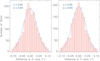 |
Fig. 1 Goodness of the distortion solution (detector #2 H-band D15 data). Differences in arcsec between the relative positions of stars in the corrected HAWK-I frames and in the VVV reference image. Left panel X-axis and right panel Y -axis. The blue lines are Gaussian fits to the histograms. For both histograms, the centre of the fit lies at 0.0 arcsec, with σ = 0.04 arcsec. |
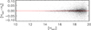 |
Fig. 2 Difference in H-band photometry before and after applying the distortion solution. The results of the photometry computed before and after the application of the distortion solution are indicated by H0 and Hcorr, respectively. This plot corresponds to detector #3 of D15 data. The units are magnitudes, with the zero point being the one specified in the HAWK-I user manual. |
2.5 Speckle holography
To produce high angular resolution images from the short exposure images, we used the speckle holography algorithm (see e.g. Primot et al. 1990; Petr et al. 1998). This requires the knowledge of the point spread function (PSF) for each short exposure. For the latter purpose, we applied the methodology described by Schödel et al. (2013), which works very well in crowded fields such as the GC. In brief, this methodology consists in the superposition of multiple reference stars and iterative improvement to determine the PSF. The image resulting from the speckle holography algorithm was convolved with a Gaussian beam of 0.2″ FWHM in order to suppress noise at high spatial frequencies. In this way we overcome the image blurring imposed by seeing. As the PSF not only varies with time but is also a function of position, mainly due to anisoplanatic effects, we divided the aligned frames into regions of 1 arcmin × 1 arcmin (from now on referred to as sub-regions). Figure 3 shows the grid of the sub-regions drawn on a long exposure image. Overlap between the sub-regions corresponds to one half of their width. Speckle holography was applied to every single sub-region independently.
The PSF for each sub-region and exposure was extracted in an automatic way. First, we generated long exposures and corresponding noise maps from all the frames corresponding to a given pointing and filter. Then, we used the StarFinder software package (Diolaiti et al. 2000) for PSF fitting astrometry and photometry. From the list of detected stars we selected reference stars for PSF extraction in each exposure according to the following criteria:
Reference stars had to be fainter than J ≈ 12, H ≈ 12, Ks ≈ 11 to avoid saturated stars. To compute these limits we performed PSF fitting photometry on the long exposure images and computed a preliminar ZP (zero point) using the SIRIUS/Infrared Survey Facility telescope (IRTF) GC survey (e.g. Nagayama et al. 2003; Nishiyama et al. 2006a). We obtained a systematic deviation for the brightest stars when we compared the ZP vs. the magnitude in the SIRIUS/IRTF GC survey. Thus, the starting point of the deviation gave us the limit for the saturation.
Reference stars had to be brighter than J = 18, H = 14, Ks = 13.
For a given exposure, the full PSF of a reference star needed to be visible, meaning stars close to the image edges were excluded.
Reference stars had to be isolated. Any neighbouring star within a distance corresponding to two times the FWHM of the seeing PSF had to be at least 2.5 mag fainter. No star brighter than the reference one was allowed within a distance corresponding approximately to the full radial extent of the PSF.
After having determined the PSF for each frame, we applied the speckle holography algorithm. Once the process was finished for each sub-region, we created the final image by combining the holographically reduced sub-regions. To do that, we performed PSF fitting astrometry and photometry (with StarFinder) for each sub-region in each band and used the positions of the detected stars to align all three bands with each other, taking as reference the H-band image. This step was important to correct small relative shifts between the sub-regions that may arise from the holography algorithm. We also produced an exposure map that informs us about the number of frames contributing to each pixel in the final image (see Fig. 4), and a noise map computed using for each pixel the error of the mean (the standard deviation of the mean divided by  , where N is the number of the measurements) of the frames that contribute to it. We produced a deep image from all the data and three so-called sub-images from three disjunct sub-sets of the data, with each one containing 1∕3 of the frames, as well as the corresponding noise maps. The sub-images were used to determine photometric and astrometric uncertainties of the detected stars as described in the next section.
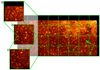 |
Fig. 3 Long exposure image (H-band chip1, D15 data) divided to obtain the sub-regions used in the holographic procedure. Region 2) corresponds to an overlapping region between 1) and 3) showing the overlapping strategy described in the text. The green lines show the division of the rest of the detector. |
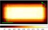 |
Fig. 4 Example of an exposure map for a final holographic product (detector #1 H-band, D15 data). The scale depicts the number of valid frames for each pixel. |
2.6 Rebinning
Since we aim to obtain final images with 0.2″ angular resolution, the sampling (0.106″ per pixel) is barely sufficient. The quality of the reconstructed images can be improved by rebinning each input frame by a factor >1 (using cubicinterpolation). The PSF fitting algorithm then can fit and disentangle the stars in this crowded field with higher accuracy. To test the optimum value of this factor and its usefulness, we simulated several hundreds of images and then applied exactly the same procedure that we followed when we reduced and analysed our science images. To do so, we selected the most difficult region that we studied in our data, namely, a square of 27″ centred on SgrA*, where the source density is the highest in the entire GC. We used a list of stars extracted from diffraction-limited Ks -band observations of the GC with NACO (NAOS-CONICA) instrument installed at the ESO VLT (S27, camera, date 9 Sept. 2012), consisting of 9840 stars with magnitudes of 9 ≲ Ks ≲ 19. This allowed us to test also the reliability of our procedure under the worst crowding conditions possible.
To generate the images, we used cubes of real PSFs from HAWK-I and we added readout and photon noise for stars and sky. Speckle holography was applied in those images using rebinning factors of 1, 2, and 3. Then, we applied the procedure described in Sect. 3 to obtain the photometry and the uncertainties of the stars. The obtained results are shown in Table 2.
As we can see, without rebinning the number of real detected sources was the lowest value obtained, whereas rebinning increased the number of detected sources significantly. To compare with the input data we discarded the outliers, removing all the stars with a photometric uncertainty >0.1 mag. A rebinning factor of 2 turned out to be a reasonable choice. Higher rebinning factors do not improve the final product significantly and may lead to additional uncertainties from interpolation. Also, computing time increases quadratically with the image size. The completeness until magnitude 15 for a rebinning factor of 2 is above 81%. We note that the completeness of our actualdata will be almost 100% at Ks ≈ 15 in less crowded regions outside the central parsec.
With respect to the photometric accuracy obtained, we compared the stellar fluxes measured in our simulations with their known input fluxes. Then, we defined a mean flux, ftot, and its associated uncertainty, dftot:
 (2)
(2)
where fHAWK−I corresponds to the flux measured in the simulated image and finput refers to the one in the input list. Once we computed those fluxes, we expressed them in magnitudes, obtaining Fig. 5. As can be seen, the photometry is slightly more accurate in the rebinned image, in particular at faint magnitudes.
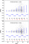 |
Fig. 5 Photometric precision for simulated data with different rebinning factors. The upper and lower panels show results for rebinning factors of 1 and 2, respectively. Blue error bars depict the standard deviation of the points in bins of one magnitude. The first row of numbers are the standard deviation in those bins. The second and third rows are the number of points used to compute the standard deviation and the number of rejected outliers. |
3 Photometry and astrometry
Stellar fluxes in the final images were measured by means of PSF fitting photometry with StarFinder. We used the noise map produced previously for the deep image, which facilitates the detection of stars and suppresses the detection of spurious sources. Since the formal uncertainties given by the StarFinder package tend to under-estimate the real uncertainties significantly (Emiliano Diolaiti, priv. comm.), we determined the error computing the photometry on the three independent sub-images.
We developed an automatic routine for PSF extraction that chooses the reference stars taking into account isolation, saturation, brightness limits (depending on the band), and weight of the stars (the number of frames contributing to the final image at a star’s position). We also excluded stars near the image edges. We used the following StarFinder parameters: a minimum correlation value of min_corr = 0.8, no diffuse background estimation, that is ESTIM_BG = 0, and a detection threshold of 5σ with two iterations.
3.1 Photometric uncertainties
We took into account two different effects for the uncertainty: statistical uncertainties and the PSF variation across the detectors.
3.1.1 Statistical uncertainties
A star was accepted only if it was detected in all three sub-images and in the deep image, using as a criterion a maximum distance of one pixel between its relative positions (corresponding to about 0.05″ because of the rebinning factor used, or about one quarter of the angular resolution). This is a conservative strategy as the deep image has a higher signal to noise ratio than the sub-images. In this way we can be certain that hardly any spurious detections will be contained in the final lists. We used the flux of a star as measured on the deep image and estimated the corresponding uncertainty, Δf, from the measurements on the three sub-images according to the formula
 (3)
(3)
where fmax and fmin correspond to the maximum and minimum flux obtained for each star in the measurements on the sub-images and N is equal to 3, the number of measurements.
We compared the formal errors provided by StarFinder on the deep image with the ones obtained with the procedure described above. We confirm that StarFinder generally under-estimates the uncertainties systematically. However, for some stars (mainly faint ones), the uncertainty given by StarFinder can be larger than the one obtained by the previous procedure. In those cases, we took the larger value, to be conservative.
3.1.2 PSF uncertainties
The PSF can potentially vary across the field. To quantify this effect, we divided the deep image horizontally into three equal regions as shown in Fig. 6. Subsequently, we obtained a PSF for each region as described above. From a comparison between the PSFs (essentially fitting the PSF from one sub-region with that from another), we estimated the corresponding photometric uncertainty and added it quadratically to the statistical uncertainties. The effect of PSF variability is only of the order of ≲2% and depends on the observing conditions.
This small effect of PSF variability highlights the excellent performance of the speckle holography algorithm. It also justifies our choice of relatively large sub-regions (1′× 1′ for the speckle holographic reconstruction). The regions are considerably larger than the size of the isoplanatic angle in the near-infrared, which is, depending on the filter used, of the order of 10″− 20″. A possible explanation why we can use such large regions is that we do not reconstruct images at the diffraction limit of the telescope, but rather at a less stringent 0.2″ FWHM. Wesuspect that we are therefore working in a “seeing-enhancer” regime, similar to ground-layer adaptive optics (GLAO) systems. GLAO corrects image degradation by turbulence in a layer close to the ground and leads therefore to moderate corrections, but over large fields (see e.g. the description of HAWK-I’s future GLAO system GRAAL, GRound layer Adaptive optics Assisted by Lasers, in Paufique et al. 2010; Arsenault et al. 2014, and references therein). We obtained the uncertainty for each individual star by adding quadratically the statistical and the PSF uncertainties. A plot of the final, combined statistical and PSF uncertainties for chip #1 is shown in Fig. 7.
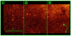 |
Fig. 6 Imagedivision of chip #1 H-band (D15) to obtain three PSFs to quantify the PSF variation across the image. Each of the numbers indicates the region considered to extract the three PSFs. |
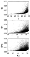 |
Fig. 7 Combined statistical and PSF photometric uncertainties vs. magnitude for J (top), H (middle), and Ks (bottom) for chip #1 (D15 data). |
3.2 Astrometric calibration
We calibrated the astrometry by using VVV catalogue stars as reference that we cross-identified with the stars detected in the images. Theastrometric solution was computed with the IDL (Interactive Data Language) routine SOLVE_ASTRO (see IDL Astronomy User’s Library, Landsman 1993).
To estimate the uncertainty of the astrometric solution, we compared all stars common to our image and to the VVV survey. Figure 8 shows the histograms of the differences in right ascension and declination. For all bands and chips the standard deviation of this distribution is ≲ 0.05 arcsec.
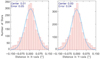 |
Fig. 8 Position accuracy. Differences in arcsec between the positions of stars in the final HAWK-I chip #4 (D15 H-band) and in the VVV reference image. Left panel X-axis and right panel Y -axis. The mean and standard deviation are 0.01 ± 0.05″ in X and 0.00 ± 0.04″ in Y. |
3.3 Zero point calibration
Since the VVV catalogue uses aperture photometry, which will lead to large uncertainties in the extremely crowded GC field, the zero point calibration was carried out relying on the catalogue from the SIRIUS/IRTF GC survey (e.g. Nagayama et al. 2003; Nishiyama et al. 2006a), which uses PSF fitting photometry. In that catalogue, the zero point was computed with an uncertainty of 0.03 mag in each band (Nishiyama et al. 2006b, 2008). To select the reference stars, we took into account several criteria:
Only stars with an uncertainty <5% in both the SIRIUS catalogue and our final list were accepted.
To avoidsaturation or faint stars, we imposed brightness limits for all three magnitudes.
The reference stars should be as isolated as possible. For that reason, we excluded all the stars which have a neighbour within a radius of 0.5″ in our final list.
-
We did not use stars near the edges of the FOV or in regions with a low number of exposures (see e.g. Fig. 4).
Finally, we applied a two-sigma clipping algorithm to remove outliers.
Figure 9 shows the zero points computed for common stars between the SIRIUS catalogue and our data in each band and chip. In all cases the reference stars were well distributed across each detector. There were also sufficient reference stars for a robust calibration: ~50 in J band, ~300 in H band, and ~175 in Ks band on each chip in the case of the 2015 data (about 30% less because of the smaller FOV in the case of the 2013 data).
We also checked for spatial variability of the zero point across the chips assuming a variable ZP and computing it with a slanting plane (i.e. a one-degree polynomial). However, we did not find any significant difference with the assumption of a constant ZP within the uncertainties. This agrees with the findings of Massari et al. (2016), who also concluded that constant zero points could be used to calibrate their HAWK-I imaging data.
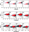 |
Fig. 9 Zero point calibration for each chip and band in D15 data. Black points represent stars common to the SIRIUS catalogue and our final list. Red points mark the stars used to compute the zero points. The mean zero points are indicated bythe blue lines. The systematic deviations for the brightest stars are due to saturation. |
3.3.1 Pistoning correction
Once the photometry obtained for every chip and band was calibrated, we corrected the possible residual zero point offset that could have remained between different chips (and pointings in the case of the 2013 data), known as “pistoning”. To do that we used the technique described in Dong et al. (2011), which consists in minimising a global χ2 that takes into account all the common stars for all chips simultaneously. For that, we only used stars with less than 0.05 mag of uncertainty. As expected, the variation in zero point between the chips was quite low (less than 0.1 mag even in the worst cases for all three bands and in both epochs). Calibrating the photometry for every chip independently with the SIRIUS catalogue before applying the pistoning correction let us compare the overlapping region of the different calibrated chips and estimate the relative offset as described in Sect. 4.
3.3.2 Combined star lists
To produce the final catalogue we merged all the photometric and astrometric measurements. For the overlap regions between the chips, the value for stars detected more than once was taken as the mean of the individual measurements. In those cases, the uncertainty was computed as the result of quadratically adding the individual uncertainties of each measurement detection. The pistoning corrections can result in minor zero point shifts of the combined star lists. To avoid them, we re-calibrated the zero point of the final, merged catalogue. This procedure was completely analogous to the one described above. Figure 10 shows the final calibration. The deviations at magnitudes Ks ≲ 11 are due to saturation.
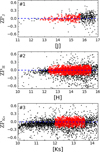 |
Fig. 10 Zero points calculated in all three bands after merging the list for every chip and pointing (D15). Black points represent allthe common stars between the SIRIUS catalogue and our data. Red points depict the stars used to compute the zero point and the blue line is its average. Systematic deviations for the brightest stars are due to saturation. |
3.3.3 Zero point uncertainty
The final ZP uncertainty was estimated by comparing the common stars of the D13 and D15 combined lists (Fig. 11). As they were calibrated independently, the photometric offset that appears between them is a measurement of the error associated with the calibration procedure. To compare the photometry, we used Eq. (2), where the fluxes are calculated from the magnitudes in both epochs. This gives us an upper limit for the uncertainties that is shown in Fig. 11. We obtained a rounded upper limit of 0.02 mag for the ZP offset between the epochs. This value takes into account possible variations of the ZP across the detector, as every star was located in a different position of the detector (or even different detectors) in both epochs. It also takes into account one of the main sources of uncertainty, namely that roughly 10% of the stars in the GC are variable (Dong et al. 2017b). Therefore, the absolute uncertainty of our catalogue results from quadratically adding this uncertainty to that of the SIRIUS catalogue. We thus obtain an absolute ZP uncertainty of 0.036 mag for each band.
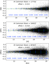 |
Fig. 11 Photometric comparison of the common stars between the final lists of D13 and D15 data obtained using Eq. (2). The green line depicts the mean of the difference between the points (we applied a two-sigma clipping algorithm to compute it). Blue lines and the number below them depict the standard deviation of the points in bins of one magnitude width. |
4 Quality assessment
To check the accuracy of the photometry, we performed several tests:
- (1)
We compared the overlapping regions of all four chips in D15 data, using Eq. (2). We excluded the borders and compared the inner regions of the overlap, where at least 100 frames contribute to each pixel (see e.g. the weight map in Fig. 4). Figure 12 shows the results for the overlap between chips #1 and #4. As can be seen, the photometric accuracy is satisfactory. The uncertainties are at most a few 0.01 mag. These independent estimates of the photometric uncertainties agree well with the combined statistical and systematic uncertainties of our final list.
- (2)
We compared the photometry from two different epochs, D13 and D15. In this case, we compared the common stars from each epoch. The overlap region is much larger than the one that we had in the previous test, so we found far more common stars, letting us improve on the quality of the analysis and extend it to the central regions of the chips. We computed uncertainty upper limits using Eq. (2) and plotted the standard deviations in bins of one magnitude in Fig. 11. The result demonstrates that the estimates of the photometric uncertainties of our finallists are accurate.
- (3)
We tookHAWK-I observations of several reference stars from the 2MASS (Two Micron All-Sky Survey) calibration Tile 92397 (RA(J2000) 170.45775 Dec(J2000) –13.22047), in all three bands, as a crosscheck to test the variability of the zero point. The calibration field was observed in a way that for each chip a reference star was positioned at nine different locations. We applied a standard reduction process to those images taking into account the special sky subtraction that we described above. Then, we performed aperture photometry for all nine positions taking four different aperture radii to test the uncertainties. All nine measurements for all the chips agree within the uncertainties with theassumption of a constant ZP across the chips.
- (4)
All the previous tests estimate the uncertainties supposing that only the detected sources are in the field. To complement the quality assessment, we used the simulations described in Sect. 2 and their corresponding uncertainties. They show the influence of extreme crowding in the photometry, as they simulated the inner parsec, which supposes the most crowed field. The photometric uncertainties that we obtained are lower because only the central region, the inner arcminute, suffers from extreme crowding. Therefore, the obtained results are consistent with this analysis.
- (5)
We qualitatively compared the Ks luminosity functions obtained with our HAWK-I data and the VVV survey. For that, we performed PSF fitting photometry with StarFinder on a final VVV mosaic centred on SgrA* observed in 2008. We produced luminosity functions for both VVV and HAWK-I data in a region of approximately 8′ × 2.5′. Figure 13 shows the results.The HAWK-I data are roughly three magnitudes deeper than the VVV data. The brightest part of the luminosity function is slightly different as a consequence of the important saturation of the Ks band in the central parsec in VVV.
Results of simulations with different rebinning factors.
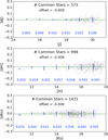 |
Fig. 12 Photometric accuracy in the overlap regions between chips #1 and #4 (D15 data). Blue lines and the number below them depict the standard deviation of the points in bins of one magnitude width. |
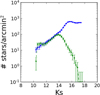 |
Fig. 13 Luminosity functions in Ks obtained with HAWK-I (blue line) and VVV (green dashed line). |
5 Colour-magnitude diagrams
Figure 14 depicts the colour-magnitude diagrams (CMD) of the D15 data. We can easily distinguish several features. The three black arrows point to foreground stellar populations that probably trace spiral arms. The highly extinguished stars lie close to or in the GC. The red ellipse indicates stars that belong to the asymptotic giant branch (AGB) bump, the red square contains ascending giant branch and post-main sequence stars, and the area marked with red dashed lines corresponds to red clump (RC) stars. They are low-mass stars burning helium in their core (Girardi 2016). Their intrinsic colours and magnitudes depend weakly on age and metallicity, so that these stars are a good tracer population to study the extinction and determine distances.
The GCfield studied here contains large dark clouds that affect significant parts of the area. In order to study the stellar population towards the GC, it therefore appears reasonable to separate areas with strong foreground extinction from those where we can look deep into the GC. Since the effect of extinction is a strong function of wavelength, dark clouds can be easily identified via the low J-band surface density of stars associated to them. This method works better than using stellar colours because those are biased towards the blue in front of dark clouds (dominated by foreground sources). The upper panel in Fig. 15 depicts the J-band surface stellar density.
To detect foreground stars and to avoid them in the subsequent analysis, we made CMDs (Ks vs. J − Ks) for regions dominated by dark clouds in the foreground of the GC, using as criterion a stellar density below 40% of the maximum density in Fig 15, and for the more transparent regions a stellar density > 75% of the maximum density. We normalised the resulting CMDs to the same area to compare them. For the transparent regions, the RC stellar population located at the GC forms a very clear clump on the right of the red dashed line in the left panel of Fig. 15. The density of foreground sources is much higher in the areas dominated by large dark clouds, as can be seen in the right panel of Fig. 15, where one of the potential spiral arms (at J − Ks ≈ 3) stands out clearly in the CMD.
The separation between the groups of stars in the foreground of dark clouds and in the deep, more transparent regions, is not unambiguous, however. Two important reasons for the overlap of the two CMDs are (1) the clumpiness of the dark clouds and (2) the large area dominated by the dark clouds. The angular size of the clumps is smaller than the smoothing length used in the stellar surface density map shown in Fig. 15. Also, we can see that the area with stellar density larger than 75% of the maximum star density is roughly only one third of the area with 40% of the maximum star density.
To confirm the existence of two groups of stars in the field, with one group highly extinguished and the other group at lower extinction, we used data from HST WFC3 (Wide Field Camera 3) centred on SgrA* with an approximate size of 2.7′ × 2.6′, to produce a CMD F153M vs. F105W – F153M (Dong et al. 2017a,b). Figure 16 shows that, when using these bands, there appears a clear gap between the two parts of the RC that we previously detected. If we select only stars that are bluer than F105W − F153M = 5.5 in the HST CMD and identify those stars in our HAWK-I list, then we obtain the CMD shown in the upper right panel of Fig. 16. On the other hand, the stars on the red side of this colour produce the CMD in thelower right panel of Fig. 16. Unfortunately, the HST data cover only a fraction of the HAWK-I FOV. However, as shown in the right panels of Fig. 16, using a colour cut at J − Ks = 5.2 we can separate fairly reliably the two giant populations with different mean extinctions.
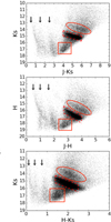 |
Fig. 14 Colour-magnitude diagrams for Ks vs. J − Ks, H vs. J − H, and Ks vs. H −Ks (D15 data). The red dashed parallelograms indicate the red clump, the red ellipse marks stars that belong to the asymptotic giant branch bump and the red square contains ascending giant branch and post-main sequence stars. The three black arrows indicate foreground stellar population probably tracing spiral arms. |
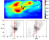 |
Fig. 15 Upper panel: J-band stellar density. Lower left panel: CMD for stars located in areas with high stellar density normalised to the same area and maximum density. Lower right panel: CMD of stars in regions dominated by dark clouds. The red dashed line approximately separates the foreground population from stars located at the Galactic centre. |
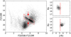 |
Fig. 16 Leftpanel: colour-magnitude diagram F153M vs. F105W – F153M. The red dashed parallelogram traces theRC and the red arrows mark an obvious gap in the distribution of the RC stars, which follows the reddening vector. The upper right panel depicts stars from our HAWK-I catalogue in J and Ks with counterpart in the HST data in the first detected bump. Analogously, the lower panel represents stars located in the second bump. |
6 Determination of the extinction curve
As outlined in the introduction, here we assume that the NIR extinction curve toward the GC can be described well by a power law of the form Aλ ∝ λ−α, where λ is the wavelength, Aλ the extinction in magnitudes at a given λ, and α is the extinction index. Here we use our data set to investigate whether α has the same value across the JHKs filters, whether it can be considered independent of the exact line of sight toward the GC, and whether it depends on the absolute value of extinction. If α can be considered a constant with respect to position, extinction, and wavelength, then we can determine its mean value. We apply several different methods to compute α and performtests of its variability.
6.1 Stellar atmosphere models plus extinction grids
We selected RC stars and assumed a Kurucz stellar atmosphere model (Kurucz 1993) with an effective temperature of 4750 K, solar metallicity, and log g = +2.5 (Bovy et al. 2014). We set the distance of the GC to 8.0 ± 0.25 kpc (Malkin 2013) and assumed a radius of 10 ± 0.5 R⊙ for the RC stars (see Chaplin & Miglio 2013; Girardi 2016, with the uncertainty given in the former reference). Then, we computed the model fluxesfor the J, H, and Ks bands assuming a grid of different values of α and the extinction at a fixed wavelength of λ = 1.61 μm, A1.61. The grid steps were 0.016 for both A1.61 and α. To convert the fluxes into magnitudes, we used a reference Vega model from Kurucz. We refer to this method as the grid method in the following text. We produced histograms to represent the distribution of the obtained parameters and fitted them with a Gaussian model. We tested different ways of computing the bin widths of the histograms. Namely, we used the Freedman-Diaconis rule (Freedman & Diaconis 1981), the Scott rule (Scott 1979), the Sturges rule (Sturges 1926), or the Doane rule (Doane 1976), among others. We did not observe any significant difference in the result of the fits. We generally adopted the Sturges rule for the histograms presented in this paper, as this rule is appropriate when the distributions to be represented are Gaussian-like. Besides, it smooths the histograms, which is convenient to overcome the segregation that can appear due to the grid step. This bin width selection criterion is applied for all the histograms presented in the paper.
We applied this method to compute α between the J and Ks bands, the H and Ks bands, the J and H bands, and across all three bands together. We defined for each star a  and searched for the parameters that minimised it.
6.1.1 RCstars in the high-extinction group
We applied the method to the RC stars with observed colours between J − Ks > 5.2 and J − Ks < 6. The histograms of the optimal values of α and A1.61, along with Gaussian fits, are shown in Figs. 17 and 18, respectively. The statistical uncertainty is given by theerror of the mean of the approximately Gaussian distributions and is negligibly small. We considered the systematic uncertainties due to the uncertainties in the temperature of the assumed model, its metallicity, the atmospheric humidity, the distance to the GC, the radius of the RC stars, and the systematics of the photometry. We re-computed the values of A1.61 and αwavelength_range varying individually the values of each of these factors:
For the model temperature we took two models with 4500 K and 5000 K. That range takes into account the possible temperature variation for the RC (Bovy et al. 2014).
For the metallicity we took five values in steps of 0.5 from –1 to +1 dex.
For the humidity we varied the amount of precipitable water vapour between 1.0, 1.6, and 3.0 mm.
For the distance to the GC, we used 7.75, 8.0, and 8.25 kpc.
We varied the stellar radius between 9.5, 10, and 10.5.
We took three different values for the logg used in the Kurucz model: 2.0, 2.5, and 3.0.
Finally, we tested the effect of the variation of the systematics of the photometry for every band independently, subtracting and adding the systematic uncertainty to all the measured values.
The largest errors arise from the uncertainty in the radius of the RC stars and the temperature of the models. The final systematic uncertainty was computed by summing quadratically all the individual uncertainties. Table 3 lists the values of α and A1.61 we obtained along with their uncertainties. We can see that αJH, αHKs, αJKs, and αJHKs are consistent within their uncertainties. On the other hand, we obtained very similar values for A1.61_JH, A1.61_HKs, and A1.61_JHKs, as we expected because we used the same stars to compute them.
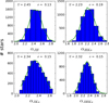 |
Fig. 17 Histograms of α computed with the grid method for the RC stars in the high-extinction group. Gaussian fits are overplotted as green lines, with the mean and standard deviations annotated in the plots. |
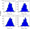 |
Fig. 18 Histograms of A1.61 computed with the grid method for the RC stars in the high-extinction group. Gaussian fits are overplotted as green lines, with the mean and standard deviations annotated in the plots. |
Values of α and A1.61 obtained with the grid method.
6.1.2 RCstars in the low-extinction group
We also applied this method to the RC stars located in front of the dark clouds, J − Ks > 4.0 and J − Ks < 5.2. Analogously, the main source of error is the systematic uncertainty, and statistical uncertainties given by the error of the mean are negligible. The Gaussian fits for the extinction index and A1.61 for JH, HKs, JKs, and JHKs are presented in Appendix A.1. Table 3 shows the results for the fits and the corresponding uncertainties.
6.1.3 All RC stars, JHKs
We also applied the previously described method to all the RC stars (J − Ks > 4 and J − Ks < 6), using JHKs measurements. We thus obtain the extinction index simultaneously for low-extinction regions and for regions dominated by dark clouds. The results are shown in Fig. 19 and in Appendix A.2. The mean values of the Gaussian fit and their uncertainties (dominated by systematics) are presented in Table 3. It can be seen that the mean and standard deviation of the histogram of the extinction indices agree very well with the values obtained for the two RC populations analysed before (Table 3). In the case of αJHKs and A1.61_JHKs, a Gaussian fit for both gives a mean value of αJHKs = 2.34 ± 0.09 and A1.61_JHKs = 3.67 ± 0.17.
On the other hand, the extinction shows a broader distribution that extends to values A1.61 < 3.4. We fitted a combination of two Gaussians and compared it with the single Gaussian fit. For that, we used the SCIKIT-LEARN python object GaussianMixture, which implements the expectation-maximisation algorithm to fit a mixture of Gaussian models (Pedregosa et al. 2011). Computing the Bayesian Information Criterion (Schwarz 1978) and the Akaike Information Criterion (Akaike 1974), we checked that a combination of two Gaussians provides a significantly better fit than using a single Gaussian. In the case of A1.61_JHKs, the mean values of the two Gaussians are A1 = 3.32 ± 0.20 and A2 = 3.88 ± 0.20, with a standard deviation of σ1 = 0.37 and σ2 = 0.29, respectively. Again, the uncertainties are dominated by the systematics. It is remarkable that the systematic uncertainties do not change the relative position of the two mean extinctions detected, since they affect both in the same direction. The mean extinctions A1 and A2 correspond to the low and highly reddened population. The results agree with their previously determined values based exclusively on each population independently. This indicates that the method is able to estimate αbands and A1.61_bands independently of the selected range of colour or extinction, distinguishing stars with different extinction. As shown in Appendix A.2, we repeated the procedure described above for JH, HKs, and JKs and found that the extinctions are compatible with a two-Gaussian model and the extinction index value is in agreement with one single αJHKs within the uncertainties of our study.
The values of the extinction indices and extinctions agree within their uncertainties. However, it is noticeable that we have found a slightly steeper value for αJH than for αHKs. Although the difference between those values is covered by the given uncertainties, the relative uncertainty between them is slightly lower. Namely, the variations in the temperature of the model, log g, the radius of the RC stars, their metallicity, and the distance to the GC produce a systematic uncertainty in the same direction for all the values computed. Therefore, we found a small difference between the extinction index depending on the wavelength in the studied ranges. This difference will be studied in detail in the next sections.
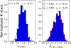 |
Fig. 19 Normalised histograms of αJHKs and A1.61 computed with all the RC stars using the grid method. The green line shows a Gaussian fit for the extinction index. The red continuous line depicts a two Gaussian fit (with the individual Gaussians marked by the red dashed lines). |
6.1.4 Spatial distribution of α
We studied the spatial variability of the extinction index, using the individual values obtained for all the RC stars in the previous section. To do that, we produced a map calculating for every pixel the corresponding value of αJHKs. To save computational time, we defined a pixel size of 100 real pixels (~5″). The value for every pixel was obtained averaging (with a two-sigma criterion) the extinction indices obtained for all the stars located within a radius of 1′ from its centre. The obtained map presents very small variations depending on the region, varying between αJHKs = 2.30 and 2.38. Fitting with a Gaussian, we obtained a mean value of αJHKs = 2.35 for all the pixels with a standard deviation of 0.03. We concluded that if there exists variation across the studied field, it is negligible. Therefore, we can assume that the extinction index does not vary with the position.
6.2 Fixed extinction
As a first estimation, a constant α from λJ to λKs can be assumed. Here, we use RC stars identified in all three bands to compute for each of them their corresponding α. To do that, we use the following expression:
 (4)
(4)
where λi refers to the effective wavelengths in each band, α is the extinction index, J, H, and Ks are the observed magnitudes in the corresponding bands, and the sub-index 0 indicates intrinsic colours (see Appendix C).
To compute the effective wavelength, λeff, and the intrinsic colours, we used as starting values the α and the A1.61 calculated in Sect. 6.1 (as explained in Appendix B). We kept A1.61 constant, but updated iteratively the values of λi and, subsequently, of α. After several iterations, the results converged. The systematic uncertainties were estimated via MonteCarlo (MC) simulations taking into account the uncertainties of the intrinsic colours, the zero points, and the effective wavelengths.
6.2.1 RCstars in the high-extinction group
We used the RC stars identified in the high-extinction group with J − Ks > 5.2 to compute the extinction index. The resulting histogram of α for all the stars is shown in Fig. 20. We obtained a value of αJHKs = 2.33 ± 0.17, where the systematic error is the main source of uncertainty and the statistical uncertainty is negligible.
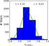 |
Fig. 20 Distribution of the extinction index for the RC stars in the high-extinction group (5.2 < J − Ks < 6) computed using Eq. (4). The green line shows a Gaussian fit, with the mean and standard deviation indicated in the legend. |
6.2.2 Spatial distribution of α
As the RC stars that we employed were well distributed across the field, we used this method to test again the constancy of the extinction index for different positions. We selected several thousands of random regions of 1.5′ radius to cover the entire field. We computed the mean α for every region and then studied the resulting distribution of values. This distribution can be described by a quasi-Gaussian distribution with a mean value of 2.35 and a small standard deviation of 0.03. This supports thenotion that α can be considered independent from the position in the field.
6.2.3 Extinction towards dark clouds
Since this method computes the extinction index based on individual stars, it is appropriate to study the stars that appear in front of dark clouds. To do that, we used the RC stars with J − Ks < 5.2 (the ones on the left part of the red line in Fig. 15) and assumed the extinction derived for this group in Sect. 6.1.2. We obtained a value of α = 2.43 ± 0.22, where the statistical uncertainty given by the error of the mean is negligible and the systematics uncertainties are the main source of error. Figure 21 shows the corresponding distribution. The slightly higher extinction index for the low-extinction stellar group can be explained by the assumption of a constant A1.61 that suffers from systematic uncertainties. That was taken into account for the error estimation and both values agree within their uncertainties.
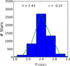 |
Fig. 21 Distribution of the extinction index for the RC stars in the low-extinction group (4.0 < J − Ks < 5.2) computed using Eq. (4). The green line shows a Gaussian fit, with the mean and standard deviation indicated in the legend. |
6.3 Colour-colour diagram
Studying the extinction index using a colour-colour diagram (CCD) removes the distance effects and arranges the RC stars in a line that follows the reddening vector. For this method, we assume that the extinction curve does not depend on extinction, which is supported by the tests in the preceding sections. By using RC stars across a broad range of extinction, a wider colour range can be used that reduces the uncertainty of the fit. Therefore, we selected RC stars with H − Ks ∈ [1.4, 2.0] and J − H ∈ [2.8, 4.0]. To computethe extinction index, we used the slope of the RC stars’s distribution in a J − H vs. H − Ks CCD. We divided the cloud of points in the CCD into bins of 0.03 mag width on the x-axis. In every bin, we used a Gaussian fit to estimate the corresponding density peak on the y-axis. The slope of the RC line and its uncertainty were subsequently computed using a Jackknife resampling method. Finally, we applied Eq. (4) to calculate the value of αJHKs. To compute the effective wavelengths, which depend on the absolute value of extinction, we assumed the value obtained with the Gaussian fit in Fig. 19.
The final result was obtained after reaching convergence through several iterations that updated the values of λi and αJHKs. We obtained αJHKs = 2.23 ±, where the uncertainty takes into account the formal uncertainty of the fit and the error due to the effective uncertainty of the wavelength. If we omitted the bluest points, where the number of stars was lower, and repeated the fit, then we obtained a value of αJHKs = 2.29 ± 0.09 as shown in Fig. 22. In both cases, the agreement with the other methods is good.
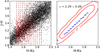 |
Fig. 22 Calculation of αJHKs using the distribution of the RC stars in the CCD. Left panel shows the cloud of points and the bins used to computed the slope. Right panel depicts the obtained points using the bins. The green line is the best fit and red contours depict the density distribution of the cloud of points. |
6.4 Obtaining α using known late-type stars
We computed the extinction index using late-type stars whose NIR K-band spectra, metallicities, and temperatures are known (Feldmeier-Krause et al. 2017). Those stars are distributed in the central 4 pc2 of the Milky Way NSC, corresponding to the central region of our catalogue. We cross-identified those stars with our catalogue and excluded stars with a photometric uncertainty <0.05 in any single band. We also excluded variable stars. For the latter purpose, we compared our D15 HAWK-I Ks -band photometry with the photometry from the D13 HAWK-I data. In that way we excluded several tens of stars that are possible variable candidates. Finally, we found 367 stars for the subsequent analysis.
6.4.1 Variable extinction
Stars whose stellar type is known let us study in detail the dependance of the extinction index on the wavelength. We used a slightly modified version of the grid method described in Sect. 6.1 to overcome the unknown radius of each used star. In this case, we defined a new  . With this approach, we do not need to know either the distance to the star or its radius.
For each star we assumed the appropriate stellar atmosphere model. We used Kurucz models because of their wide range of metallicities and temperatures, which was necessary to analyse properly the data. We varied the metallicity in steps of 0.5 dex from −1 to 1 dex. The temperature of the models was 3500 K, 4000 K, and 4500 K, consistent with the uncertainty in temperature for each star (~ 200 K in average). Because the lower limit for the model temperatures was 3500 K, we deleted ten stars that were not covered by any model.
Becausethis method has only one known variable, the colour, we cannot compute simultaneously the extinction and the extinction index. Thus, we computed the individual extinction of each star using the measured colour J − Ks. We minimised the difference between the data and the theoretical colour obtained using the appropriate Kurucz model (taking into account the metallicity and the temperature) and a grid of extinctions, A1.61, with a step of 0.01 mag. For that, we used the extinction index derived in Sect. 6.1. We obtained a quasi-Gaussian distribution for the extinction that is shown in the left panel of Fig. 23. The systematic uncertainty dominates the errors whereas the statistical uncertainty is negligible. We computed the systematics taking into account the variation of the extinction index (using the uncertainties computed in Sect. 6.1), the systematic uncertainty of the ZP, and different amounts of precipitable water vapour (1.0, 1.6, and 3.0 mm). We ended up with a mean extinction of A1.61 = 4.28 ± 0.18. We used J − Ks because to convert colour into extinction, we need to assume a value of α to compute the grid of individual extinctions and, for that wavelength range, the value is similar to the one obtained assuming a constant extinction index for all the three bands (see Sect. 6.1) and we do not need to assume different values for the ranges J − H and H − Ks. In this way, we computed the extinction for each star and fixed it to compute the extinction index. Figure 24 and Table 4 summarise the obtained results. The statistical uncertainties, given by the error of the mean, are negligible, and the systematic uncertainties are the main source of error. To compute them, we took into account the systematics introduced by the zero points, the initial α used to translate the colour J − Ks into extinction, and the humidity of the atmosphere.
 |
Fig. 23 Left panel: A1.61 distribution computed individually for each spectroscopically studied late-type star. Right panel: α estimated using the fixed extinction method for the same stars. The green line shows a Gaussian fit, with the mean and standard deviation indicated in the legend. |
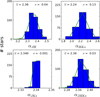 |
Fig. 24 Histograms of α computed with the modified grid method for known late-type stars. Gaussian fits are overplotted as green lines, with the mean and standard deviations annotated in the plots. |
Values of α obtained with the modified grid method for known late-type stars.
6.4.2 Fixed extinction
We employed the same approach described above (Sect. 6.2). In this case, we used the fixed extinction given by the Gaussian fit shown in Fig. 23 (left panel). To obtain the final αJHKs, we used an iterative approach updating the value of the extinction index obtained in every step until reaching convergence. To start the iterations we used the extinction index derived in Sect. 6.1.3. The resulting distribution of αJHKs is shown in Fig. 23 (right panel). The estimation of the systematic uncertainty was carried out considering the systematics of the ZP, the possible variation of the fixed extinction, and different amounts of precipitable water vapour (1.0, 1.6, and 3.0 mm). The final result was αJHKs = 2.12 ± 0.14, which is in agreement with all the previous estimates. The slightly lower extinction index obtained can be explained by the assumption of a constant A1.61, which suffers from systematic uncertainties. That was taken into account in the uncertainty estimation.
6.5 Computing the extinction index using early-type stars
We used again the same methods described in Sect. 6.4 to compute the extinction index towards known hot, massive stars near Sgr A* (Do et al. 2009). We used the D13 data, which cover the central region far better than the D15 data. We excluded known Wolf-Rayet stars (Paumard et al. 2006; Do et al. 2009; Feldmeier-Krause et al. 2015) because they are frequently dusty and therefore intrinsically reddened. To avoid spurious identifications because of the high crowding of the region, we only used stars with 11.2≤ Ks ≤ 13. We used the published NACO Ks magnitudes (approximately equivalent to the HAWK-I Ks band) and compared them with our HAWK-I data applying a 3-σ exclusion criterion to delete any possible variable stars. Finally, we excluded stars with photometric uncertainties larger than 0.05 mag in any single band. We ended up with 23 accepted stars for the analysis.
6.5.1 Variable extinction
As described in Sect. 6.4.1, we applied the modified grid method and computed the individual extinction to each star to analyse the variation of the extinction index with the wavelength. We used a 30 000 K model, a solar metallicity, a log g = 4.0, and a humidity of 1.6 mm of precipitable water vapour. The uncertainties were estimated using the error of the mean of the quasi-Gaussian distribution and varying the parameters previously described to obtain the systematics. The final mean value is A1.61_JKs = 4.61 ± 0.20, where 0.13 and 0.16 correspond to the statistical and systematic uncertainties. Figure 25 (left panel) shows the obtained results. Figure 26 and Table 4 present the obtained results for the modified grid method.
We found again the variation in the extinction index that we already noticed in Sect. 6.1.3. This supports the evidence of having a steeper extinction index between J and H than between H and Ks. However, the difference between the extinction indices and the uncertainties that we found is not enough to clearly distinguish two different values. Therefore, we estimate that, in spite of being different, their close values make necessary a deeper analysis with better spectral resolution or wide wavelength coverage, to clearly distinguish them. Within the limits of the current study, we assume that a constant extinction index is enough to describe the extinction curve between the analysed bands.
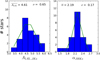 |
Fig. 25 Left panel: A1.61 distribution computed individually for each spectroscopically studied late-type star. Right panel: α estimated using the fixed extinction method for the same stars. The green line shows a Gaussian fit, with the mean and standard deviation indicated in the legend. |
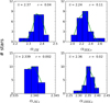 |
Fig. 26 Histograms of α computed with the modified grid method for known early-type stars. Gaussian fits are overplotted as green lines, with the mean and standard deviations annotated in the plots. |
6.5.2 Fixed extinction
A Kurucz model with a temperature of 30 000 K and solar metallicity was taken to compute αJHKs. We used the mean value obtained above and presented in Fig. 25 (left panel). The result is shown in Fig. 25 (right panel). The systematic uncertainty dominates the error and was computed using MC simulations considering the uncertainties in the ZP calibration of all three bands, the effective wavelength, and the intrinsic colour of J − H and H − Ks. The final value was αJHKs = 2.19 ± 0.13, which is consistent with the values determined by the other methods.
6.6 Finalextinction index value and discussion
Given our results from all the different methods to estimate the extinction index on our data, we can conclude that all the derived values of α agree withintheir uncertainties and that there is no evidence - within the limits of our study - for any variation of α with position, or absolute value of interstellar extinction. On the other hand, we observed a small dependence with the wavelength when we considered different values for αJH and αHKs. However, a constant extinction index, αJHKs, seems to be sufficient to describe the extinction curve. We average all the values obtained with the different methods explained above and obtain a final value αJHKs = 2.30 ± 0.08, where the uncertainty is given by the standard deviation of the measurements, which takes into account the dispersion of the values obtained using the different methods.
To check the reliability of the obtained value for the extinction index, we used all the RC stars identified in Fig. 14 and computed their radii using the individual extinction for each star and the derived extinction index. We used the colour J − Ks to calculate the individual extinctions employing the grid approach described in Sect. 6.4.1. Then, we computed the corresponding radius for each star assuming the final extinction index, the GC distance (8.0 kpc, Malkin 2013) and a Kurucz model for Vega to convert the fluxes into magnitudes. We obtained the radius by comparing the obtained value with the measured Ks of each star. Figure 27 depicts the obtained individual extinctions (left panel) and the derived radius (right panel). We obtained a value of A1.61 = 3.78 ± 0.15 and r = 10.03 ± 0.57 R⊙, where the error is dominated by the systematic uncertainty. The comparison between the obtained extinction and the one computed in Sect. 6.1, and shown in Fig. 19, is consistent. Moreover, we have obtained a mean radius for the RC stars that agrees perfectly with the standard value of 10.0 ± 0.5 R⊙ (Chaplin & Miglio 2013; Girardi 2016). Therefore, we conclude that the computed values for the extinction and the extinction index are consistent and let us calculate the radius of the RC stars obtaining an accurate value.
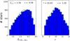 |
Fig. 27 Left panel: A1.61_JKs distribution computed for all the RC stars. Right panel: radii distribution of the RC stars (in solar radii). The green line shows a Gaussian fit, with mean and standard deviation indicated in the legend. |
7 A highangular resolution extinction map
To produce an AKs extinction map, we removed all the foreground population and kept only the RC stars indicated by the parallelogram in Fig. 14 and detected in H and Ks bands. The observed colours were converted into extinction using the colour H − Ks (as we have far more stars detected in H and Ks than in J) and the following equation:
 (5)
(5)
where the subindex 0 refers to the intrinsic colour and λi are the effective wavelengths.
To save computational time, we defined a pixel scale of 0.5″/pixel for the extinction map. For every pixel, we computed the extinction using the colour of the ten closest stars, limiting the maximum distance to 12″ from its centre. If less than ten stars were found for a pixel, we did not assign any extinction value to avoid obtaining strongly biased values due to too distant stars. To take into account the different distances of the stars to every pixel, we computed the colour using an inverse distance weight (IDW) method. Namely, we weighted every star based on the distance to the corresponding pixel following the expression:
 (6)
(6)
where v is the magnitude to be computed in the target pixel, d is the distance to that pixel, vi are the known values, and p is the weight factor. We explored different values for p and ended up with p = 0.25 as the best estimate to avoid giving too much weight to the star closest to the pixel centre.
The uncertainty of the extinction map was computed estimating the colour uncertainty of every pixel, using a Jackknife algorithm in the calculation of the IDW. The resulting extinction map and its corresponding uncertainty map are shown in Fig. 28. The mean uncertainty is ~ 5%. Besides, we estimate a systematic error of ~5%, which takes into account the uncertainties of the effective wavelengths and the extinction index.
Due to the fact that the extinction can vary on scales of arcsec, we tried to improve the extinction map using not only the RC stars, but all stars with Ks between 12 and 17, and H − Ks between 1.4 and 3.0. In this way, we almost duplicate the number of selected stars, improving significantly the angular resolution of the map. To compute the intrinsic colour of every star, we assumed that the majority of the used stars can be considered as giants. We calculated the Ks reddened magnitude of several Kurucz models of giants (assuming an average extinction of 3.67 mag at 1.61 μm, see Sect. 6.1) and their intrinsic colour. We interpolated the points to build a smooth function that gives the intrinsic colour based on the measured Ks magnitude (see Fig. 29). The resulting extinction map and its corresponding uncertainty map are shown in Fig. 30. It can be seen that it is very similar to Fig. 28, but with a higher angular resolution. The statistical and systematic uncertainties are similar as well.
With this approach, we generated, in addition, two more extinction maps taking into account the two groups of stars that we identified in Sect. 5. Namely, we produced the first map using stars with 1.4 < H − Ks < 1.7 (Fig. 31, upper panel) and the second one with stars between 1.7 < H − Ks < 3.0 (Fig. 31, lower panel). In this way, the first map represents the extinction screen toward the foreground population (excluding stars in the spiral arms), whereas the second one includes the interstellar extinction all the way toward GC stars. Although the first map does show some correlation with the second map (e.g. in regions 1, 2, 3) because it is impossible to separate the two stellar populations without any overlap, it shows a rather constant extinction, with a mean of 1.72 and a standard deviation of 0.06. This demonstrates that this foreground screen can be considered to vary on very large scales. The statistical and systematic uncertainties for this first extinction map are ~ 2% and ~6%, respectively.In this case the uncertainty is lower because we consider a narrower range in H − Ks and all the stars are closer without mixing stars with different extinctions. On the other hand, the second map contains fine structure on scales of just a few arcsec, which is consistent with the extinction being caused by a clumpy medium close to the GC. The statistical and systematic uncertainties of the map are ~ 4% and ~ 5%, respectively.
When comparing the extinction map in the lower panel of Fig. 31 with the J-band density plot (Fig. 15), we can see that the high density regions, marked with numbers 1, 2, and 3, correspond to low extinction as we expected. However, while region 4 can be identified as a high-extinction region in the density plot, it appears as a low-extinction one in the lower panel of 31, but as a relatively high-extinction region in the upper panel. We interpret this as evidence for a large dark cloud with very high densitythat blocks most of the light from the stars behind it. This is also rather evident from inspecting a JHKs colour image of our field (Fig. 32). We conclude that our method cannot produce reliable extinction maps for regions marked by the presence of highly opaque foreground clouds.
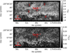 |
Fig. 28 Upper panel: extinction map AKS obtained using all the RC stars shown in Fig. 14. Lower panel: corresponding uncertainty map. The numbers in red indicate regions to be compared between the different extinction maps (see main text). |
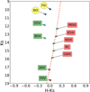 |
Fig. 29 Reddened observed magnitude (assuming a distance modulus of 14.51 and a mean extinction A1.61 = 3.67) vs. intrinsic colour for several types of stars computed using Kurucz models. The red dashed line indicates the intrinsic colours usedfor the stars selected to compute the extinction map. |
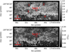 |
Fig. 30 Upper panel: extinction map AKs obtained using stars with 12 < Ks < 17 and 1.4 < H − Ks < 3.0. Lower panel: corresponding uncertainty map. The numbers in red indicate regions to be compared between the different extinction maps (see main text). |
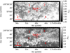 |
Fig. 31 Upper panel: extinction map for stars with observed colours in the interval 1.4 < H − Ks < 1.7. Lower panel: extinction map for stars with observed colours in the interval 1.7 < H − Ks < 3. The numbers in red indicate regions to be compared between the different extinction maps (see main text). |
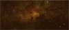 |
Fig. 32 RGBimage of Field 1 (red for Ks, green for H, and blue for J). |
8 Stellar populations
8.1 CMDs
To obtain a rough idea of the stellar populations in Field 1 of our survey, we attempted to deredden the CMD. We transformed the AKs extinction maps into AH using the RC effective wavelength and the extinction index of αJHKs = 2.30, as determined by us. We used the two extinction maps computed previously according to the different H − Ks colours. This enabled us to improve the dereddening process as we considered two different maps that correspond to two different layers in the line of sight. We used either one or the other, depending on the H − Ks colour of a given star. The divisions were 1.4 < H − Ks < 1.7 and 1.7 < H − Ks < 3.0, which is similar to the J − Ks cut in Fig. 16. Figure 33 shows the CMDs for Ks vs. H − Ks before and after de-reddening. Analogously, we repeated the process for J band but, in this case, we produced the extinction maps taking into account only stars identified in all three bands, J, H, and Ks. By doing so, we obtain a consistent extinction map and avoid producing extinction maps biased towards too high extinction, as the completeness is higher in H and Ks than in J. Figure 34 depicts the CMD Ks versus J − Ks before and after de-reddening. It can be seen that the extinction correction clearly reduces the scatter in the CMDs. On the other hand, we overplotted different Kurucz stellar models. The giant sequence follows clearly the main density ridge in both dereddened CMDs. In both cases, Ks vs. H − Ks and Ks vs. J − Ks, the standard deviation of the dereddened colours around the giant branch is of the order of σ = 0.2.
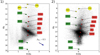 |
Fig. 33 Panel 1 shows the CMD Ks vs. H −Ks. We have overplotted several Kurucz stellar models (assuming a mean extinction A1.61 =3.97, see Sect. 6.1) to identify the expected position of those stars. Panel 2 depicts the dereddened map once we have applied the extinction maps. Both panels have different scales on the X-axis. |
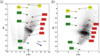 |
Fig. 34 Panel 1: CMD Ks vs. J − Ks. We have overplotted several Kurucz stellar models (assuming a mean extinction A1.61 =3.97, see Sect. 6.1) to identify the expected position of those stars. Panel 2: dereddened map once we have applied the extinction maps. Both panels have different scales on the X-axis. |
8.2 CMD modelling
We overplotted three 5 Gyr isochrones (Marigo et al. 2017) with different metallicities (0.1, 1, and 2.5 solar metallicity) to the CMD Ks vs. J − Ks. In this way we are able to compare them with the stellar population. We can clearly see how a super-solar metallicity population fits better the data on the right hand side of the CMD. This is in particular indicated by the centring of the AGB bump. The RC bump appears to be centred at lower metallicities, but that is an effect of extinction and completeness, because the RC clump is cut off at the red end of the JKs CMD. Therefore, a range of solar metallicities around the solar metallicity can explain the observed data. This is in agreement with the low number of low metallicity stars found in the central 4 pc2 in Feldmeier-Krause et al. (2017). On the other hand, the scatter of the stars in the upper part of the diagram gives us an idea of the goodness of the extinction correction ~0.2, explaining the difference in comparison with the isochrones. This is the first study that infers the GC metallicity by using only photometricdata.
The right panel of Fig. 35 shows a synthetic model population in comparison with the real data. The model assumes 2.5 solar metallicity and two different age intervals, from 1 Gyr < t < 5 Gyr and from 5 Gyr < t < 12 Gyr. In both cases the star formation rate is constant over the time. The synthetic population was created analogously as described in Pfuhl et al. (2011), using the code of Aparicio & Gallart (2004) that used the stellar evolution library from Bertelli et al. (1994) and the bolometric correction library from Lejeune et al. (1997). It can be seen that taking into account the uncertainty that produces the scatter of around 0.2 mag, we are able to reproduce several features observed in the data like the RC bump or the AGB branch. Therefore, within the limits of the current study, we suggest that a solar or super-solar metallicity explains well the observed stellar distribution.
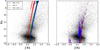 |
Fig. 35 Left panel: 5 Gyr stellar isochrones with different metallicities overlaid on the CMD Ks vs. J − Ks. Right panel: comparison of the real data in the CMD Ks vs. J − Ks with asynthetic stellar model produced using the code of Aparicio & Gallart (2004), a metallicity of 2.5 solar metallicity, and a constant stellar formation between 1 Gyr <t < 5 Gyr (blue circles)and 5 Gyr < t < 12 Gyr (red diamonds). |
9 Discussion and conclusions
We have presented the observations, data reduction, and the analysis for Field 1 of our GALACTICNUCLEUS survey. Using HAWK-I at the ESO VLT with short readout times, we applied the speckle holography algorithm to create JHKs images with a PSF FWHM of 0.2″. This allows us to obtain accurate photometry in the crowded field of the GC. Our 5σ sensitivity limits are approximately J = 22, H = 21, and Ks = 20. The photometric uncertainty is <0.05 mag at J ≲ 20, H ≲ 17, and Ks ≲ 16. The uncertainty of the zero points is 0.036 mag in each band. The angular resolution and sensitivity of our data allows us to reach well below the important tracer population of red clump stars in all three bands, except in highly reddened areas in J.
We identify three stellar populations in the foreground, at low extinction, with mean observed H − Ks ≈ 0.2, 0.5, 0.8, which we interpret to belong to spiral arms along the line of sight. At the distance of the GC, we identify a high-extinction population, with a mean H − Ks ≈ 2.0, and a population at somewhat lower extinction at H − Ks ≈ 1.5. Both populations appear clearly distinct in an HST/WFC3 F105W − F153M vs. F153M CMD and can be separated relatively cleanly using a colour threshold of J − Ks = 5.2. Since the RC of the low-extinction population lies along the reddening line of the more extinguished RC, we believe that the low-extinction population lies approximately at the distance of the GC. As a tentative explanation, we hypothesise that we are seeing stars in front of the dust and molecular gas of the central molecular zone (CMZ). This is in agreement with the findings of Launhardt et al. (2002) that about 80% of the molecular gas in the CMZ appears to be concentrated in a torus with radii between 120 to 220 pc. The clumpiness of the ISM in the CMZ (see also Launhardt et al. 2002) will, of course, complicate this simple picture.
Our deep and sensitive data allow us to study the NIR extinction curve during the GC in unprecedented detail. We found some evidence for a possible difference in the extinction index between J − H and H − Ks. However, it is small and the extinction index can be assumed to be roughly constant within the limits of our study. Moreover, the value found here, αJHKs = 2.30 ± 0.08, is in excellent agreement with the latest literature values on the NIR extinction curve towards the GC. Nishiyama et al. (2006a) found αJHKs = 2.23 ± 0.23 (value taken from Table 5 in Fritz et al. 2011), Schödel et al. (2010) found αJHKs = 2.21 ± 0.24, and Fritz et al. (2011) found αJHKs = 2.11 ± 0.06. The study carried out by Stead & Hoare (2009) found αJHKs = 2.14 ± 0.05 not towards the GC but towards eight regions of the Galaxy between l ~ 27° and ~ 100°. Zasowski et al. (2009) also found a compatible αJHKs = 2.26 ± 0.17 (value taken from Table 5 in Fritz et al. 2011) towards different regions of the Milky Way (over nearly 150° of contiguous Milky Way midplane longitude). This may indicate a universal value for αJHKs that is steeper than assumed in older work (e.g. Rieke & Lebofsky 1985; Draine 1989; Cardelli et al. 1989). Besides, Stead & Hoare (2009) also point out that great care must be taken in the choice of the filter wavelength when using broadband filters. This has been done in the current work by computing carefully the effective wavelengths accordingly, as shown in Appendix B.
We studied possible variations of αJHKs with position in the field and with the absolute value of extinction, but cannot find any evidence for any such dependence, as suggested, for example, by Gosling et al. (2009), who found a broad range for αJHKs in the GC with a strong dependency on the line of sight. We believe that the latter work suffered from crowding and low angular resolution, which limited the authors to make assumptions on the median properties of their observed stellar populations. They could not select specifically RC stars and had to rely on median colours of stars in their fields. Hence, we claim that the NIR extinction curve toward the GC can be approximated by a power law with constant index αJHKs.
Such a well-behaved extinction curve can facilitate the next step of our analysis: the attempt to identify hot, massive stars in the GC, which can provide evidence for the star formation history in the past few 100 Myr. On the other hand, we have created several extinction maps and have identified a first layer of low varying extinction and a second one closer to the GC where the extinction varies in arcsec scales. Therefore, it appears that a significant part of the extinction toward the GC is originated from a highly clumpy medium near the GC. The clumpiness is in agreement with previous studies of the ISM in the CMZ (e.g. Launhardt et al. 2002). This division enables us to improve the de-reddening process to obtain more accurate de-reddened CMDs. Using them, we have employed isochrones with different metallicities (Marigo et al. 2017) and a synthetic stellar model (Aparicio & Gallart 2004) to infer the metallicity of the stellar population in the studied region. We found that a solar to super-solar metallicity fits the data well. This study supposes the first time that metallicity has been guessed using only photometry in the near infrared for the GC.
This is the first of a series of papers that will present and exploit the GALACTICNUCLEUS survey. It is supported by an ESO Large Programme and all images and source catalogues will be made publicly available.
Acknowledgements
The research leading to these results has received funding from the European Research Council under the European Union’s Seventh Framework Programme (FP7/2007-2013)/ERC grant agreement No. [614922]. This work is based on observations made with ESO Telescopes at the La Silla Paranal Observatory under programmes IDs 195.B-0283 and 091.B-0418. We thank the staff of ESO for their great efforts and helpfulness. F.N.-L. acknowledges financial support from a MECD pre-doctoral contract, code FPU14/01700. F.N. acknowledges Spanish grants FIS2012-39162-C06-01, ESP2013-47809-C3-1-R and ESP2015-65597-C4-1-R. This work has made use of the IAC-STAR Synthetic CMD computation code. IAC-STAR is supported and maintained by the computer division of the Instituto de Astrofísica de Canarias.
Appendix A Extinction and extinction index analysis. Plots and fits
A.1 Grid method. RC stars. Low extinction
Figures A.1 and A.2 show the results obtained applying the methodology described in Sect. 6.1.1 to the low extinguished RC stars.
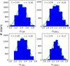 |
Fig. A.1 Histograms of α computed with the grid method for the low-extinction group of RC stars. Gaussian fits are overplotted as green lines, with the mean and standard deviations annotated in the plots. |
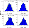 |
Fig. A.2 Histograms of A1.61 computed with the grid method for the low-extinction group of RC stars. Gaussian fits are overplotted as green lines, with the mean and standard deviations annotated in the plots. |
A.2 Grid method. All RC stars
Figures A.3 and A.4 show the results obtained applying the methodology described in Sect. 6.1.3 to all the RC stars.
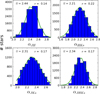 |
Fig. A.3 Histograms of α computed with the grid method for all the RC stars. Gaussian fits are overplotted as green lines, with the mean and standard deviations annotated in the plots. |
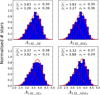 |
Fig. A.4 Normalised histograms of A1.61 computed with the grid method for all the RC stars. The red continuous line shows two-Gaussian fits and the red dashed lines show the individual Gaussians of the fit. The mean and standard deviations of the fits are annotated in the plots. |
Appendix B Effectivewavelength
To compute the effective wavelength, λeff, we used Eq.(A3) of Tokunaga & Vacca (2005). We used the transmission curves for the HAWK-I J, H, and Ks filters from the instrument website and the atmospheric transmission from the Gemini telescope web site. Because the λeff was computed for several stellar types (RC stars, late-type stars with known metallicity and temperature, and young stars), we used the more adequate Kurucz model for every case. We took the extinction index and A1.61 obtained with the grid method described in Sect. 6.1, being the value specified in every section accordingly.
Effective wavelength and uncertainties for RC stars.
Effective wavelength and uncertainties for known young stars.
To calculate α we used an iterative approach in some of the methods. In those cases, we recomputed λeff using the α that was obtained in the first step and repeated the process updating the value until reaching convergence. The uncertainties for every λeff were estimated varying the parameters that affect them in their uncertainty ranges. In that way, we computed λeff varying the same parameter and keeping the rest constant. We considered:
The temperature of the model. For the RC stars, we used 4500, 4750, and 5000 K. For the known young stars we used 20 000, 30 000, and 40 000 K.
The metallicity of the model. We varied for all the cases from −1 dex to +1 dex in steps of 0.5.
We took three different values for the logg that we used in the Kurucz model: for RC, 2.0, 2.5, and 3.0, and for the young known stars 3.5, 4.0, and 4.5.
The amount of precipitable water vapour. We used 1.0, 1.6, and 3.0 mm.
The extinction index and A1.61. We varied them according to the value and uncertainties obtained in Sect. 6.1.
The final uncertainty was computed adding quadratically all the uncertainties. The final value was computed using the central parameters that were described for the uncertainties. Then, 4750 K and 30 000 K, solar metallicity, and 1.6 mm of precipitable water vapour were used for the final values of the λeff for RC stars and young stars, respectively. Tables B.1 and B.2 summarise the effective wavelength and the uncertainties for the high extinguished RC stars and young stars. The largest error came from α and A1.61. In the case of late-type stars with known metallicity, we applied an individual model for each of them.
Appendix C Intrinsic colour calculation
The intrinsic colours (J−H)0 and (H−Ks)0 were computed using the appropriate Kurucz models for each type of star. We took into account the transmission curves for the HAWK-I J, H, and Ks filters from the instrument web site and the atmospheric transmission from the Gemini telescope web site. We computed the total magnitude for every band and then normalised it using a Vega reference model (Kurucz model). As in the calculation of λeff, and taking the same values, we estimate the uncertainty varying the parameters that affect the intrinsic colour calculation (temperature of the model, metallicity, logg, and precipitable water vapour). The values for RC stars and young known stars are presented in Tables C.1 and C.2. For RC stars we used a model with solar metallicity, 4750 K, and 1.6 mm of precipitable water vapour. For the young known stars, we only changed the temperature of the model to 30 000 K. As in Appendix B, the final uncertainty was computed adding quadratically all the individual uncertainties. In this way, we obtained an upper limit for the uncertainty. It can be seen that the most important factor is the temperature of the model. In the case of known late-type stars, we computed for each of them the corresponding value, depending on the metallicity and temperature.
Intrinsic colour for RC stars.
Intrinsic colour for known young stars.
References
- Akaike, H. 1974, Automatic Control, IEEE Trans., 19, 716 [Google Scholar]
- Aparicio, A., & Gallart, C. 2004, AJ, 128, 1465 [NASA ADS] [CrossRef] [Google Scholar]
- Arsenault, R., Paufique, J., Kolb, J., et al. 2014, The Messenger, 156, 2 [NASA ADS] [Google Scholar]
- Bertelli, G., Bressan, A., Chiosi, C., Fagotto, F., & Nasi, E. 1994, A&AS, 106 [Google Scholar]
- Bovy, J., Nidever, D. L., Rix, H.-W., et al. 2014, ApJ, 790, 127 [NASA ADS] [CrossRef] [Google Scholar]
- Cardelli, J. A., Clayton, G. C., & Mathis, J. S. 1989, ApJ, 345, 245 [NASA ADS] [CrossRef] [Google Scholar]
- Chaplin, W. J., & Miglio, A. 2013, ARA&A, 51, 353 [NASA ADS] [CrossRef] [Google Scholar]
- Diolaiti, E., Bendinelli, O., Bonaccini, D., et al. 2000, A&AS, 147, 335 [NASA ADS] [CrossRef] [EDP Sciences] [Google Scholar]
- Do, T., Ghez, A. M., Morris, M. R., et al. 2009, ApJ, 703, 1323 [NASA ADS] [CrossRef] [Google Scholar]
- Doane, D. P. 1976, The American Statistician, 30, 181 [NASA ADS] [Google Scholar]
- Dong, H., Wang, Q. D., Cotera, A., et al. 2011, MNRAS, 417, 114 [NASA ADS] [CrossRef] [Google Scholar]
- Dong, H., Lacy, J. H., Schödel, R., et al. 2017a, MNRAS, 470, 561 [NASA ADS] [CrossRef] [Google Scholar]
- Dong, H., Schodel, R., Williams, B. F., et al. 2017b, MNRAS, 471, 3617 [NASA ADS] [CrossRef] [Google Scholar]
- Draine, B. T. 1989, in Infrared Spectroscopy in Astronomy, ed. E. Böhm-Vitense, ESA Spec. Publ., 290, 93 [NASA ADS] [Google Scholar]
- Feldmeier-Krause, A., Neumayer, N., Schödel, R., et al. 2015, A&A, 584, A2 [NASA ADS] [CrossRef] [EDP Sciences] [Google Scholar]
- Feldmeier-Krause, A., Kerzendorf, W., Neumayer, N., et al. 2017, MNRAS, 464, 194 [NASA ADS] [CrossRef] [Google Scholar]
- Freedman, D., & Diaconis, P. 1981, Probability Theory and Related Fields, 57, 453 [Google Scholar]
- Fritz, T. K., Gillessen, S., Dodds-Eden, K., et al. 2011, ApJ, 737, 73 [NASA ADS] [CrossRef] [Google Scholar]
- Genzel, R., Eisenhauer, F., & Gillessen, S. 2010, Rev. Mod. Phys., 82, 3121 [NASA ADS] [CrossRef] [Google Scholar]
- Girardi, L. 2016, ARA&A, 54, 95 [NASA ADS] [CrossRef] [EDP Sciences] [Google Scholar]
- Gosling, A. J., Bandyopadhyay, R. M., & Blundell, K. M. 2009, MNRAS, 394, 2247 [NASA ADS] [CrossRef] [Google Scholar]
- Kissler-Patig, M., Pirard, J.-F., Casali, M., et al. 2008, A&A, 491, 941 [NASA ADS] [CrossRef] [EDP Sciences] [Google Scholar]
- Kurucz, R. L. 1993, VizieR Online Data Catalog, 6039, 0 [Google Scholar]
- Landsman, W. B. 1993, in Astronomical Data Analysis Software and Systems II, eds. R. J. Hanisch, R. J. V. Brissenden, & J. Barnes, ASP Conf. Ser., 52, 246 [NASA ADS] [Google Scholar]
- Launhardt, R., Zylka, R., & Mezger, P. G. 2002, A&A, 384, 112 [NASA ADS] [CrossRef] [EDP Sciences] [Google Scholar]
- Lejeune, T., Cuisinier, F., & Buser, R. 1997, A&AS, 125, 229 [NASA ADS] [CrossRef] [EDP Sciences] [Google Scholar]
- Malkin, Z. 2013, in IAU Symp., 289, ed. R. de Grijs, 406 [Google Scholar]
- Marigo, P., Girardi, L., Bressan, A., et al. 2017, ApJ, 835, 77 [NASA ADS] [CrossRef] [Google Scholar]
- Massari, D., Fiorentino, G., McConnachie, A., et al. 2016, A&A, 595, L2 [NASA ADS] [CrossRef] [EDP Sciences] [Google Scholar]
- Minniti, D., Lucas, P. W., Emerson, J. P., et al. 2010, New A, 15, 433 [Google Scholar]
- Nagayama, T., Nagashima, C., Nakajima, Y., et al. 2003, in Instrument Design and Performance for Optical/Infrared Ground-based Telescopes, eds. M. Iye & A. F. M. Moorwood, Proc. SPIE, 4841, 459 [NASA ADS] [CrossRef] [Google Scholar]
- Nishiyama, S., Nagata, T., Kusakabe, N., et al. 2006a, ApJ, 638, 839 [NASA ADS] [CrossRef] [Google Scholar]
- Nishiyama, S., Nagata, T., Sato, S., et al. 2006b, ApJ, 647, 1093 [NASA ADS] [CrossRef] [Google Scholar]
- Nishiyama, S., Nagata, T., Tamura, M., et al. 2008, ApJ, 680, 1174 [NASA ADS] [CrossRef] [Google Scholar]
- Paufique, J., Bruton, A., Glindemann, A., et al. 2010, in Adaptive Optics Systems II, Proc. SPIE, 7736, 77361P [CrossRef] [Google Scholar]
- Paumard, T., Genzel, R., Martins, F., et al. 2006, ApJ, 643, 1011 [NASA ADS] [CrossRef] [Google Scholar]
- Pedregosa, F., Varoquaux, G., Gramfort, A., et al. 2011, J. Mach. Lear. Res., 12, 2825 [Google Scholar]
- Petr, M. G., Coude Du Foresto, V., Beckwith, S. V. W., Richichi, A., & McCaughrean, M. J. 1998, ApJ, 500, 825 [NASA ADS] [CrossRef] [Google Scholar]
- Pfuhl, O., Fritz, T. K., Zilka, M., et al. 2011, ApJ, 741, 108 [NASA ADS] [CrossRef] [Google Scholar]
- Primot, J., Rousset, G., & Fontanella, J. C. 1990, J. Opt. Soc. Am. A, 7, 1598 [NASA ADS] [CrossRef] [Google Scholar]
- Reid, M. J., & Brunthaler, A. 2004, ApJ, 616, 872 [NASA ADS] [CrossRef] [Google Scholar]
- Rieke, G. H., & Lebofsky, M. J. 1985, ApJ, 288, 618 [NASA ADS] [CrossRef] [Google Scholar]
- Saito, R. K., Minniti, D., Dias, B., et al. 2012, A&A, 544, A147 [NASA ADS] [CrossRef] [EDP Sciences] [Google Scholar]
- Schödel, R., Najarro, F., Muzic, K., & Eckart, A. 2010, A&A, 511, A18 [NASA ADS] [CrossRef] [EDP Sciences] [Google Scholar]
- Schödel, R., Yelda, S., Ghez, A., et al. 2013, MNRAS, 429, 1367 [NASA ADS] [CrossRef] [Google Scholar]
- Schödel, R., Feldmeier, A., Neumayer, N., Meyer, L., & Yelda, S. 2014, Class. Quant. Grav., 31, 244007 [NASA ADS] [CrossRef] [Google Scholar]
- Schwarz, G. 1978, Ann. Stat., 6, 461 [Google Scholar]
- Scott, D. W. 1979, Biometrika, 66, 605 [CrossRef] [MathSciNet] [Google Scholar]
- Scoville, N. Z., Stolovy, S. R., Rieke, M., Christopher, M., & Yusef-Zadeh, F. 2003, ApJ, 594, 294 [Google Scholar]
- Stead, J. J., & Hoare, M. G. 2009, MNRAS, 400, 731 [NASA ADS] [CrossRef] [Google Scholar]
- Sturges, H. A. 1926, J. Am. Stat. Assoc., 21, 65 [Google Scholar]
- Tokunaga, A. T., & Vacca, W. D. 2005, PASP, 117, 421 [NASA ADS] [CrossRef] [Google Scholar]
- Zasowski, G., Majewski, S. R., Indebetouw, R., et al. 2009, ApJ, 707, 510 [Google Scholar]
Based on observations made with ESO telescopes at the La Silla Paranal Observatory under programme ID 195.B-0283.
All Tables
All Figures
|
Fig. 1 Goodness of the distortion solution (detector #2 H-band D15 data). Differences in arcsec between the relative positions of stars in the corrected HAWK-I frames and in the VVV reference image. Left panel X-axis and right panel Y -axis. The blue lines are Gaussian fits to the histograms. For both histograms, the centre of the fit lies at 0.0 arcsec, with σ = 0.04 arcsec. |
| In the text | |
|
Fig. 2 Difference in H-band photometry before and after applying the distortion solution. The results of the photometry computed before and after the application of the distortion solution are indicated by H0 and Hcorr, respectively. This plot corresponds to detector #3 of D15 data. The units are magnitudes, with the zero point being the one specified in the HAWK-I user manual. |
| In the text | |
|
Fig. 3 Long exposure image (H-band chip1, D15 data) divided to obtain the sub-regions used in the holographic procedure. Region 2) corresponds to an overlapping region between 1) and 3) showing the overlapping strategy described in the text. The green lines show the division of the rest of the detector. |
| In the text | |
|
Fig. 4 Example of an exposure map for a final holographic product (detector #1 H-band, D15 data). The scale depicts the number of valid frames for each pixel. |
| In the text | |
|
Fig. 5 Photometric precision for simulated data with different rebinning factors. The upper and lower panels show results for rebinning factors of 1 and 2, respectively. Blue error bars depict the standard deviation of the points in bins of one magnitude. The first row of numbers are the standard deviation in those bins. The second and third rows are the number of points used to compute the standard deviation and the number of rejected outliers. |
| In the text | |
|
Fig. 6 Imagedivision of chip #1 H-band (D15) to obtain three PSFs to quantify the PSF variation across the image. Each of the numbers indicates the region considered to extract the three PSFs. |
| In the text | |
|
Fig. 7 Combined statistical and PSF photometric uncertainties vs. magnitude for J (top), H (middle), and Ks (bottom) for chip #1 (D15 data). |
| In the text | |
|
Fig. 8 Position accuracy. Differences in arcsec between the positions of stars in the final HAWK-I chip #4 (D15 H-band) and in the VVV reference image. Left panel X-axis and right panel Y -axis. The mean and standard deviation are 0.01 ± 0.05″ in X and 0.00 ± 0.04″ in Y. |
| In the text | |
|
Fig. 9 Zero point calibration for each chip and band in D15 data. Black points represent stars common to the SIRIUS catalogue and our final list. Red points mark the stars used to compute the zero points. The mean zero points are indicated bythe blue lines. The systematic deviations for the brightest stars are due to saturation. |
| In the text | |
|
Fig. 10 Zero points calculated in all three bands after merging the list for every chip and pointing (D15). Black points represent allthe common stars between the SIRIUS catalogue and our data. Red points depict the stars used to compute the zero point and the blue line is its average. Systematic deviations for the brightest stars are due to saturation. |
| In the text | |
|
Fig. 11 Photometric comparison of the common stars between the final lists of D13 and D15 data obtained using Eq. (2). The green line depicts the mean of the difference between the points (we applied a two-sigma clipping algorithm to compute it). Blue lines and the number below them depict the standard deviation of the points in bins of one magnitude width. |
| In the text | |
|
Fig. 12 Photometric accuracy in the overlap regions between chips #1 and #4 (D15 data). Blue lines and the number below them depict the standard deviation of the points in bins of one magnitude width. |
| In the text | |
|
Fig. 13 Luminosity functions in Ks obtained with HAWK-I (blue line) and VVV (green dashed line). |
| In the text | |
|
Fig. 14 Colour-magnitude diagrams for Ks vs. J − Ks, H vs. J − H, and Ks vs. H −Ks (D15 data). The red dashed parallelograms indicate the red clump, the red ellipse marks stars that belong to the asymptotic giant branch bump and the red square contains ascending giant branch and post-main sequence stars. The three black arrows indicate foreground stellar population probably tracing spiral arms. |
| In the text | |
|
Fig. 15 Upper panel: J-band stellar density. Lower left panel: CMD for stars located in areas with high stellar density normalised to the same area and maximum density. Lower right panel: CMD of stars in regions dominated by dark clouds. The red dashed line approximately separates the foreground population from stars located at the Galactic centre. |
| In the text | |
|
Fig. 16 Leftpanel: colour-magnitude diagram F153M vs. F105W – F153M. The red dashed parallelogram traces theRC and the red arrows mark an obvious gap in the distribution of the RC stars, which follows the reddening vector. The upper right panel depicts stars from our HAWK-I catalogue in J and Ks with counterpart in the HST data in the first detected bump. Analogously, the lower panel represents stars located in the second bump. |
| In the text | |
|
Fig. 17 Histograms of α computed with the grid method for the RC stars in the high-extinction group. Gaussian fits are overplotted as green lines, with the mean and standard deviations annotated in the plots. |
| In the text | |
|
Fig. 18 Histograms of A1.61 computed with the grid method for the RC stars in the high-extinction group. Gaussian fits are overplotted as green lines, with the mean and standard deviations annotated in the plots. |
| In the text | |
|
Fig. 19 Normalised histograms of αJHKs and A1.61 computed with all the RC stars using the grid method. The green line shows a Gaussian fit for the extinction index. The red continuous line depicts a two Gaussian fit (with the individual Gaussians marked by the red dashed lines). |
| In the text | |
|
Fig. 20 Distribution of the extinction index for the RC stars in the high-extinction group (5.2 < J − Ks < 6) computed using Eq. (4). The green line shows a Gaussian fit, with the mean and standard deviation indicated in the legend. |
| In the text | |
|
Fig. 21 Distribution of the extinction index for the RC stars in the low-extinction group (4.0 < J − Ks < 5.2) computed using Eq. (4). The green line shows a Gaussian fit, with the mean and standard deviation indicated in the legend. |
| In the text | |
|
Fig. 22 Calculation of αJHKs using the distribution of the RC stars in the CCD. Left panel shows the cloud of points and the bins used to computed the slope. Right panel depicts the obtained points using the bins. The green line is the best fit and red contours depict the density distribution of the cloud of points. |
| In the text | |
|
Fig. 23 Left panel: A1.61 distribution computed individually for each spectroscopically studied late-type star. Right panel: α estimated using the fixed extinction method for the same stars. The green line shows a Gaussian fit, with the mean and standard deviation indicated in the legend. |
| In the text | |
|
Fig. 24 Histograms of α computed with the modified grid method for known late-type stars. Gaussian fits are overplotted as green lines, with the mean and standard deviations annotated in the plots. |
| In the text | |
|
Fig. 25 Left panel: A1.61 distribution computed individually for each spectroscopically studied late-type star. Right panel: α estimated using the fixed extinction method for the same stars. The green line shows a Gaussian fit, with the mean and standard deviation indicated in the legend. |
| In the text | |
|
Fig. 26 Histograms of α computed with the modified grid method for known early-type stars. Gaussian fits are overplotted as green lines, with the mean and standard deviations annotated in the plots. |
| In the text | |
|
Fig. 27 Left panel: A1.61_JKs distribution computed for all the RC stars. Right panel: radii distribution of the RC stars (in solar radii). The green line shows a Gaussian fit, with mean and standard deviation indicated in the legend. |
| In the text | |
|
Fig. 28 Upper panel: extinction map AKS obtained using all the RC stars shown in Fig. 14. Lower panel: corresponding uncertainty map. The numbers in red indicate regions to be compared between the different extinction maps (see main text). |
| In the text | |
|
Fig. 29 Reddened observed magnitude (assuming a distance modulus of 14.51 and a mean extinction A1.61 = 3.67) vs. intrinsic colour for several types of stars computed using Kurucz models. The red dashed line indicates the intrinsic colours usedfor the stars selected to compute the extinction map. |
| In the text | |
|
Fig. 30 Upper panel: extinction map AKs obtained using stars with 12 < Ks < 17 and 1.4 < H − Ks < 3.0. Lower panel: corresponding uncertainty map. The numbers in red indicate regions to be compared between the different extinction maps (see main text). |
| In the text | |
|
Fig. 31 Upper panel: extinction map for stars with observed colours in the interval 1.4 < H − Ks < 1.7. Lower panel: extinction map for stars with observed colours in the interval 1.7 < H − Ks < 3. The numbers in red indicate regions to be compared between the different extinction maps (see main text). |
| In the text | |
|
Fig. 32 RGBimage of Field 1 (red for Ks, green for H, and blue for J). |
| In the text | |
|
Fig. 33 Panel 1 shows the CMD Ks vs. H −Ks. We have overplotted several Kurucz stellar models (assuming a mean extinction A1.61 =3.97, see Sect. 6.1) to identify the expected position of those stars. Panel 2 depicts the dereddened map once we have applied the extinction maps. Both panels have different scales on the X-axis. |
| In the text | |
|
Fig. 34 Panel 1: CMD Ks vs. J − Ks. We have overplotted several Kurucz stellar models (assuming a mean extinction A1.61 =3.97, see Sect. 6.1) to identify the expected position of those stars. Panel 2: dereddened map once we have applied the extinction maps. Both panels have different scales on the X-axis. |
| In the text | |
|
Fig. 35 Left panel: 5 Gyr stellar isochrones with different metallicities overlaid on the CMD Ks vs. J − Ks. Right panel: comparison of the real data in the CMD Ks vs. J − Ks with asynthetic stellar model produced using the code of Aparicio & Gallart (2004), a metallicity of 2.5 solar metallicity, and a constant stellar formation between 1 Gyr <t < 5 Gyr (blue circles)and 5 Gyr < t < 12 Gyr (red diamonds). |
| In the text | |
|
Fig. A.1 Histograms of α computed with the grid method for the low-extinction group of RC stars. Gaussian fits are overplotted as green lines, with the mean and standard deviations annotated in the plots. |
| In the text | |
|
Fig. A.2 Histograms of A1.61 computed with the grid method for the low-extinction group of RC stars. Gaussian fits are overplotted as green lines, with the mean and standard deviations annotated in the plots. |
| In the text | |
|
Fig. A.3 Histograms of α computed with the grid method for all the RC stars. Gaussian fits are overplotted as green lines, with the mean and standard deviations annotated in the plots. |
| In the text | |
|
Fig. A.4 Normalised histograms of A1.61 computed with the grid method for all the RC stars. The red continuous line shows two-Gaussian fits and the red dashed lines show the individual Gaussians of the fit. The mean and standard deviations of the fits are annotated in the plots. |
| In the text | |
Current usage metrics show cumulative count of Article Views (full-text article views including HTML views, PDF and ePub downloads, according to the available data) and Abstracts Views on Vision4Press platform.
Data correspond to usage on the plateform after 2015. The current usage metrics is available 48-96 hours after online publication and is updated daily on week days.
Initial download of the metrics may take a while.