| Issue |
A&A
Volume 609, January 2018
|
|
|---|---|---|
| Article Number | A136 | |
| Number of page(s) | 30 | |
| Section | Extragalactic astronomy | |
| DOI | https://doi.org/10.1051/0004-6361/201730844 | |
| Published online | 05 February 2018 | |
The Carnegie Supernova Project I
Analysis of stripped-envelope supernova light curves⋆,⋆⋆
1 Department of Astronomy, The Oskar Klein Center, Stockholm University, AlbaNova, 10691 Stockholm, Sweden
e-mail: This email address is being protected from spambots. You need JavaScript enabled to view it.
2 Department of Physics and Astronomy, Aarhus University, Ny Munkegade 120, 8000 Aarhus C, Denmark
3 Facultad de Ciencias Astronómicas y Geofísicas, Universidad Nacional de La Plata, Paseo del Bosque S/N, B1900 FWA La Plata, Argentina
4 Instituto de Astrofísica de La Plata (IALP), CONICET, Argentina
5 Kavli Institute for the Physics and Mathematics of the Universe, Todai Institutes for Advanced Study, University of Tokyo, 5-1-5 Kashiwanoha, Kashiwa, Chiba 277-8583, Japan
6 Homer L. Dodge Department of Physics and Astronomy, University of Oklahoma, 440 W. Brooks, Rm 100, Norman, OK 73019-2061, USA
7 Observatories of the Carnegie Institution for Science, 813 Santa Barbara St., Pasadena, CA 91101, USA
8 Las Campanas Observatory, Carnegie Observatories, Casilla 601, La Serena, Chile
9 Department of Physics, Florida State University, 77 Chieftain Way, Tallahassee, FL 32306, USA
10 George P. and Cynthia Woods Mitchell Institute for Fundamental Physics and Astronomy, Department of Physics and Astronomy, Texas A&M University, College Station, TX 77843, USA
Received: 22 March 2017
Accepted: 22 August 2017
Abstract
Stripped-envelope (SE) supernovae (SNe) include H-poor (Type IIb), H-free (Type Ib), and He-free (Type Ic) events thought to be associated with the deaths of massive stars. The exact nature of their progenitors is a matter of debate with several lines of evidence pointing towards intermediate mass (Minit< 20 M⊙) stars in binary systems, while in other cases they may be linked to single massive Wolf-Rayet stars. Here we present the analysis of the light curves of 34 SE SNe published by the Carnegie Supernova Project (CSP-I) that are unparalleled in terms of photometric accuracy and wavelength range. Light-curve parameters are estimated through the fits of an analytical function and trends are searched for among the resulting fit parameters. Detailed inspection of the dataset suggests a tentative correlation between the peak absolute B-band magnitude and Δm15(B), while the post maximum light curves reveals a correlation between the late-time linear slope and Δm15. Making use of the full set of optical and near-IR photometry, combined with robust host-galaxy extinction corrections, comprehensive bolometric light curves are constructed and compared to both analytic and hydrodynamical models. This analysis finds consistent results among the two different modeling techniques and from the hydrodynamical models we obtained ejecta masses of 1.1–6.2M⊙, 56Ni masses of 0.03–0.35M⊙, and explosion energies (excluding two SNe Ic-BL) of 0.25–3.0 × 1051 erg. Our analysis indicates that adopting κ = 0.07 cm2 g-1 as the mean opacity serves to be a suitable assumption when comparing Arnett-model results to those obtained from hydrodynamical calculations. We also find that adopting He i and O i line velocities to infer the expansion velocity in He-rich and He-poor SNe, respectively, provides ejecta masses relatively similar to those obtained by using the Fe ii line velocities, although the use of Fe ii as a diagnostic does imply higher explosion energies. The inferred range of ejecta masses are compatible with intermediate mass (MZAMS ≤ 20M⊙) progenitor stars in binary systems for the majority of SE SNe. Furthermore, our hydrodynamical modeling of the bolometric light curves suggests a significant fraction of the sample may have experienced significant mixing of 56Ni, particularly in the case of SNe Ic.
Key words: supernovae: general
Based on observations collected at Las Campanas Observatory.
Bolometric light curve tables are only available at the CDS via anonymous ftp to cdsarc.u-strasbg.fr (130.79.128.5) or via http://cdsarc.u-strasbg.fr/viz-bin/qcat?J/A+A/609/A136
© ESO, 2018
1. Introduction
Stripped-envelope (SE) core-collapse supernovae (SNe) are associated with the deaths of massive stars that have experienced significant mass loss over their evolutionary lifetimes. The severity of the mass loss drives to first order the contemporary spectroscopic classification sequence of Type IIb → Ib → Ic (e.g., Filippenko 1997; Gal-Yam 2017; Prentice & Mazzali 2017; Shivvers et al. 2017). The progenitors of SN IIb are thought to retain a residual amount (~0.01 M⊙) of hydrogen prior to exploding, and as an outcome they exhibit hydrogen features in pre-maximum spectra. However, soon after maximum (tmax) their spectra typically evolve to resemble normal SNe Ib (e.g., SN 1993J; Filippenko et al. 1993), exhibiting conspicuous helium features and only traces (if any signatures at all) of hydrogen. Rounding out the spectroscopic sequence are SNe Ic, which lack hydrogen and helium spectral features, and in some instances show exceedingly broad-lined (BL) spectral features. Some SNe Ic-BL have been discovered to emerge from long-duration gamma-ray bursts (e.g., SN 1998bw; Galama et al. 1998).
A large number of single-object studies of SE SNe exist, especially of events that occurred in nearby galaxies. Historical examples of a SE SNe that were comprehensively studied in single-object papers are SN IIb 1993J (Filippenko et al. 1993, 1994), SN Ib 2008D (Soderberg et al. 2008; Mazzali et al. 2008; Modjaz et al. 2009; Malesani et al. 2009; Bersten et al. 2013), SN Ic 1994I (Filippenko et al. 1995), and SN Ic-BL 1998bw (Galama et al. 1998; Patat et al. 2001).
The light curves of SE SNe are mainly powered by thermalized energy originating from the radioactive decay chain 56Ni →56Co →56Fe. Given the amount of 56Ni synthesized in SE SNe, their relatively low ejecta masses, and the compact radii of their progenitors, they almost always display bell-shaped light curves peaking a few weeks after explosion. For a handful of cases the SE SNe were discovered within hours to days after explosion. In some of these cases an initial peak has been documented, followed by a rapid drop in luminosity. This early emission is believed to be driven by the shock wave breaking out through the progenitor’s surface or through an extended envelope surrounding the progenitor (e.g., Arnett & Falk 1976; Ensman & Burrows 1992; Woosley et al. 1994; Bersten et al. 2012; Piro & Nakar 2013; Nakar & Piro 2014; Piro 2015). The early luminosity is mainly dependent on the progenitor radius. Evidence of this phenomenon was first documented in the peculiar Type II SN 1987A (e.g., Catchpole et al. 1987), the Type IIb SN 1993J (e.g., Van Driel et al. 1993), the Type Ib/c SN 1999ex (Stritzinger et al. 2002), and the Type Ib SN 2008D (e.g., Mazzali et al. 2008; Soderberg et al. 2008). Recently, with the advent of both amateur and professional transient surveys, a handful of additional SE SNe have been discovered in the midst of their initial peak/adiabatic-cooling phase, including for example: SN 2009K (Stritzinger et al. 2018a), SN 2011hs (Bufano et al. 2014), SN 2011dh (Arcavi et al. 2011), PTF11mnb (Taddia et al. 2018), and iPTF15dtg (Taddia et al. 2016).
In recent years, several studies have presented expanded SE SN samples. Richardson et al. (2006) presented the analysis of a sample of V-band light curves for 27 SE SNe. Drout et al. (2011) published the first multi-band (V and R bands) sample of SNe Ib/c, studying 25 SNe; more recently, Bianco et al. (2014), Modjaz et al. (2014), and Liu et al. (2016) have published optical and near-infrared light curves and visual-wavelength spectroscopy of >60 SE SNe followed by the Center for Astrophysics (CfA) SN group. Taddia et al. (2015) studied the ugriz light curves of a sample of 20 SNe Ib/c obtained by the Sloan-Digital-Sky-Survey II (SDSS-II) SN survey. Additionally, Cano (2013), Lyman et al. (2016), and Prentice et al. (2016) have used large SE SN samples (61, 38, and 85 SNe, respectively) based on collections of optical data from the literature to constrain explosion and progenitor properties. From these studies, SE SNe are found to be characterized by relatively small average ejecta masses (Mej) ranging between 1–5 M⊙, average explosion energies (EK) of a few 1051 erg, and average 56Ni masses of ≈0.1–0.3 M⊙. Hydrodynamical modeling of several specific SE SNe indicate similar values for the explosion properties. For example, SN 2011dh, modeled by Bersten et al. (2012) and Ergon et al. (2014), was characterized by Mej = 1.8–2.5 M⊙, energy 0.6–1.0 × 1051erg, and 56Ni mass of 0.05–0.10 M⊙. Furthermore, light-curve and spectral modeling reveal that in several cases the 56Ni is mixed into the outer SN ejecta (e.g., Bersten et al. 2012; Cano et al. 2014; Taddia et al. 2015). As compared to SNe IIb, Ib, and Ic, SNe Ic-BL are generally characterized by higher EK and larger 56Ni masses (see, e.g., Cano 2013; Taddia et al. 2015; Lyman et al. 2016).
The fact that SE SNe generally have small ejecta masses suggests a large fraction of them do not arise from very massive stars (>25–30 M⊙), whose mass-loss rates would not be high enough to strip most of the outer layers and leave these low ejecta masses. Therefore, it is more likely that they arise from binary systems, where the SN progenitor is an intermediate-mass star (MZAMS ≲ 20 M⊙) that experiences significant mass loss to its companion over its evolutionary lifetime (see, e.g., Yoon et al. 2015, and references therein). In the case of SN 1993J, the companion was even identified in images a decade after its explosion (Maund et al. 2004; Fox et al. 2014). Furthermore, a possible detection of the companion of SN 2011dh’s progenitor star was suggested by Folatelli et al. (2014a). The SN iPTF13bvn was the first SN Ib whose progenitor (a relatively low-mass star) was detected (Cao et al. 2013; Fremling et al. 2014), as recently confirmed by its disappearance in Hubble Space Telescope (HST) post-explosion observations (Folatelli et al. 2016; Eldridge & Maund 2016).
The analysis of late-phase nebular spectra of SE SNe also indicates relatively low-mass progenitors, particularly in the case of SNe IIb (Jerkstrand et al. 2015). Specifically, mass constraints of SE SN progenitors obtained from oxygen-abundance determinations by modeling late-phase spectroscopy point towards progenitors characterized by MZAMS≈ 12–13M⊙ (see, e.g., Jerkstrand et al. 2015). This is corroborated by the lack of detections of bright Wolf-Rayet (WR) stars in pre-explosion images of nearby SE SNe (Eldridge et al. 2013), as well as by the relatively high rate of SE SNe (Smith et al. 2011; Shivvers et al. 2017). However, a few SE SNe with large ejecta masses (corresponding to broad light curves) have been suggested, such as SN 2005bf (e.g., Folatelli et al. 2006), SN 2011bm (Valenti et al. 2012), iPTF15dtg (Taddia et al. 2016), PTF11mnb (Taddia et al. 2018), and SN 2012aa (Roy et al. 2016). These objects could have possibly arisen from massive (MZAMS> 30 M⊙) single stars.
Studies of the environments of SE SNe suggested a difference in metallicity between SNe Ib and Ic, with the latter being richer in metals (Anderson et al. 2010; Modjaz et al. 2011). This suggests an important role for line-driven winds in the stripping of the SE SN progenitors, as naturally expected for single massive stars. However, other works did not confirm this difference (Leloudas et al. 2011; Sanders et al. 2012).
Between 2004 and 2009 the Carnegie Supernova Project (CSP-I; Hamuy et al. 2006) conducted follow-up observations of over two hundred SNe using mainly facilities at Las Campanas Observatory (LCO). A chief aim of the CSP-I was to construct a SE SN sample obtained on a homogeneous, stable, and well-understood photometric system. By the completion of the CSP-I follow-up program, optical broad-band observations of 34 spectroscopically classified SE SNe were obtained, with a subset of 26 objects having at least some near-infrared (NIR) imaging. Definitive photometry of the sample is presented by Stritzinger et al. (2018a), while additional companion papers by Stritzinger et al. (2018b) and Holmbo et al. (in prep.) study the color/reddening properties and visual-wavelength spectroscopy, respectively. In this paper we present the analysis of the light-curve properties and construct comprehensive bolometric light curves, which are used to estimate key explosion parameters via semi-analytical and hydrodynamical modeling.
We stress that an overall goal of the CSP-I is to obtain photometry of a variety of SNe types on a stable, homogeneous, and well-understood photometric system. Fortunately, the stability of the observing conditions offered by LCO and its facilities, combined with our dedication to leave no stone unturned in our efforts to understand the CSP-I photometry system (see Krisciunas et al. 2017), enabled the computation of photometry with an accuracy and wavelength coverage unparalleled in other samples. Another important aspect of our work is the combination of the accurate photometry of the CSP-I SE SN sample with robust host-galaxy reddening corrections, which we have studied in a dedicated paper (see Stritzinger et al. 2018b). The wavelength coverage and the host-reddening corrections allowed us to construct comprehensive UltraViolet-Optical-near-InfraRed (UVOIR) bolometric light curves, which are modeled using both semi-analytical and hydrodynamical modeling. The consistency of the inferred explosion parameters between the two methods is also investigated. An important limitation in the determination of the explosion parameters is the relatively large uncertainty associated to the explosion epoch for the majority of the events, which we discuss in Sect. 6.1.
The organization of this paper is as follows. Section 2 provides a brief summary of the CSP-I SE SN sample, including pertinent details regarding each SN. Section 3 contains the detailed analysis of the light-curve shape properties. This is followed by Sect. 4, which examines the absolute magnitudes. Subsequently, in Sect. 5 spectral energy distributions (SEDs) are used to construct UVOIR light curves, from which progenitor and explosion parameters are estimated in Sect. 6. Finally, a discussion on our results is presented in Sect. 7 and conclusion are given in Sect. 8.
2. The CSP-I stripped-envelope supernova sample
Table 1 contains the list of the 34 SE SNe followed by the CSP-I (Stritzinger et al. 2018a). Twenty-nine of the objects have ugriBV-band light curves, five objects lack u-band photometry (i.e., SN 2004ew, SN 2006bf, SN 2007ag, SN 2007rz, and SN 2009dp), and 26 objects have YJH-band photometry.
CSP-I SE SN sample.
The sample consists of 10 SNe IIb, 11 SNe Ib, and 13 SNe Ic, with the classification of all of the objects based on visual-wavelength spectra obtained by the CSP-I (Holmbo et al., in prep.). Among the SN Ib sub-sample is the peculiar SN 2005bf, which is characterized by a prominent second peak, which has never been seen before in these objects. Given its uniqueness, it is omitted from our light-curve analysis. However, a detailed study of it based on CSP-I light curves and spectroscopy has been presented by Folatelli et al. (2006), in addition to earlier papers by Anupama et al. (2005) and Tominaga et al. (2005). In addition, among the SN Ic sub-sample both SN 2009bb (Pignata et al. 2011) and SN 2009ca are broad-lined objects. Beside SN 2005bf and 2009bb, the CSP-I data of SN 2007Y were published and analyzed in a single object paper by Stritzinger et al. (2009). A number of SNe in our sample were observed by other groups or included in literature sample analyses. In Table 1 we marked the eighteen SNe which were also observed by Bianco et al. (2014), which is the sample with which we have the largest number of SNe in common.
Basic information for each SN and its host galaxy were compiled using the NASA/IPAC Extragalactic Database (NED) and the Asiago Supernova Catalog (Barbon et al. 1999), and compiled into Table 1. This includes SN designation, coordinates and spectral type, host-galaxy designation and coordinates, Galactic visual extinction, redshift, and distance. Values are also provided for semi-major and semi-minor axes, morphological type, and position angle (PA) of the host galaxy, as well as the de-projected SN distance from the host-galaxy center.
Milky Way extinction values ( , where X corresponds to a given passband) are obtained from NED1’s listings of the Schlafly & Finkbeiner (2011) recalibration of the Schlegel et al. (1998) dust maps. Host-galaxy reddening values are estimated through the comparison of observed optical and NIR colors to intrinsic color-curve templates constructed from sub-samples of minimally-reddened CSP-I SE SNe (Stritzinger et al. 2018b). Nine minimally-reddened events were selected among those with no or little Na i D absorption, with the observed bluest B−V color at ten days past peak, located far from their host-galaxy centers, and in galaxies which are not strongly tilted. For seven highly-reddened objects, we directly determined the reddening parameter
  and the
  extinction by fitting their measured color excesses with a Fitzpatrick (1999, hereafter F99) reddening law. These values are taken from Stritzinger et al. (2018b, last two columns of their Table 3). For objects suffering lower amounts of extinctions, we adopted the average value listed in Stritzinger et al. (2018b, last column of their Table 4).
As explained by Stritzinger et al. (2018b), the values used differ for each of the SE SN subtypes. Specifically, for SNe Ib suffering low reddening we adopt the value obtained from the most reddened member of this subtype (i.e., SN 2007C). This approach is also followed for the other SE SN subtypes. As demonstrated in Stritzinger et al. (2018b), nine objects are identified to be minimally-reddened and they are used to construct intrinsic color-curve templates. When the photometry of an object could not be used to estimate the reddening via comparison of observed and intrinsic color due to poor follow-up, we instead turn to estimates obtained from the equivalent width of the Na i D (EWNa i D) feature. Combining the EWNa i D measurements (Stritzinger et al. 2018b, their Table 1) and the relation between this quantity and as derived in Stritzinger et al. (2018b) (i.e., ![Mathematical equation: \hbox{$A_V^{\rm host}~{\rm[mag]} = 0.78 \cdot EW_{\ion{Na}{i}{\rm ~D}}$}](/articles/aa/full_html/2018/01/aa30844-17/aa30844-17-eq56.png) [Å]), we obtain an estimate of the host extinction. We note that Phillips et al. (2013) showed that estimating extinction (even in our galaxy) via EWNa i D implies large uncertainty. The adopted values of and for each SE SN are summarized in Table 1.
[Å]), we obtain an estimate of the host extinction. We note that Phillips et al. (2013) showed that estimating extinction (even in our galaxy) via EWNa i D implies large uncertainty. The adopted values of and for each SE SN are summarized in Table 1.
The listed redshifts and direct distance estimates are from the NED and NED-D catalogs. Direct distance measurements are adopted (mainly obtained through the Tully-Fisher method) when available. If not, NED-based luminosity distances are adopted assuming cosmological parameters Ωm = 0.27, ΩΛ = 0.73 (Komatsu et al. 2009), and H0 = 73.8 ± 2.4 km s-1 Mpc-1 (Riess et al. 2011), and corrections for peculiar velocity based on Virgo, Great Attractor (GA), and Shapley flow models (Mould et al. 2000).
NED also provides values for the major (2a) and minor (2b) galaxy diameters, while the morphological t-type and PA of each galaxy are adopted from the Asiago Supernova Catalog (Barbon et al. 1999). Following Hakobyan et al. (2009, 2012), de-projected and diameter-normalized SN distances from the host-galaxy center (dSN) were computed and are listed in the last column of Table 1. In this table we also report the values of the galaxy diameters, position angles, and coordinates, as well as the SN coordinates that we used to compute the de-projected and diameter-normalized distances. These parameters allowed us to confirm that each of the minimally-reddened SE SNe was located far from its host’s center (see Stritzinger et al. 2018b).
In the following, all the light curves are corrected for time dilation and K corrected. Given the redshifts of the SNe, the time dilation corrections are <3%, with the exception of SNe 2008gc and 2009ca whose time corrections are ≈5% and ≈10%, respectively. The K corrections were computed following the method described by Hsiao et al. (2007). The visual-wavelength K corrections were calculated using the Nugent SN Ibc spectral template2. As the Nugent templates extend out to +70 d and spectral features evolve slowly at late time, we use the last spectrum for anything beyond this epoch. At NIR wavelengths, K corrections were computed using the NIR spectroscopic time series of SN 2011dh (Ergon et al. 2014). In the vast majority of objects, the K corrections are on the order of <0.05 mag in the V band, with the median of all the K correction in the V band being 0.03 mag. Oates et al. (2012) found similar V-band K correction values for the Type IIb SN 2009mg located at z = 0.0076, which is about half of the median redshift range of the CSP-I sample.
3. Light-curve shape properties
3.1. Light-curve fits
The broad wavelength coverage afforded by the CSP-I SE SN sample enables the light-curve shapes to be studied in nine photometric passbands extending from u to H band. To facilitate comparison of the various filtered light curves among the entire sample, each filtered light curve was fit with an analytic function. The adopted function works well with decently time-sampled SN follow-up, providing a continuous description of the data and a set of parameters describing the shape of the light curve that are useful for comparison.
The shape of SE SN light curves can be represented in terms of three components consisting of: (i) an initial exponential rise; (ii) a Gaussian-like peak; and (iii) a late linear decay. The functional form of the analytic function is expressed as ![Mathematical equation: \begin{equation} m(t)=\frac{y_0+m(t-t_0)+g_0 {\rm exp}[-(t-t_0)^2/2\sigma_0^2]}{1-{\rm exp}[(\tau-t)/\theta]}\cdot \label{eq:1} \end{equation}](/articles/aa/full_html/2018/01/aa30844-17/aa30844-17-eq65.png) (1)Here y0 is the intercept of the linear decline, characterized by slope m. The final term in the numerator corresponds to the Gaussian-peak, normalized to phase (t0), amplitude (g0), and width (σ0). The denominator corresponds to the exponential rise, where θ is a characteristic time, and τ is a separate phase zero-point. This function was originally introduced by Vacca & Leibundgut (1996) to study the light-curve properties of thermonuclear supernovae (see additional applications to SN Ia studies in papers by Contardo et al. 2000; and Stritzinger 2005).
(1)Here y0 is the intercept of the linear decline, characterized by slope m. The final term in the numerator corresponds to the Gaussian-peak, normalized to phase (t0), amplitude (g0), and width (σ0). The denominator corresponds to the exponential rise, where θ is a characteristic time, and τ is a separate phase zero-point. This function was originally introduced by Vacca & Leibundgut (1996) to study the light-curve properties of thermonuclear supernovae (see additional applications to SN Ia studies in papers by Contardo et al. 2000; and Stritzinger 2005).
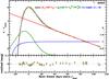 |
Fig. 1 Best fit of Eq. (1)(black solid line) to the r-band light curve (triangles) of SN 2006T normalized to its peak brightness. The three components of the analytic fit are shown: blue for the exponential rise, green for the Gaussian peak, and red for the linear decay. The corresponding terms in Eq. (1)are color-coded accordingly. The residuals between the fit and the photometry are plotted in the bottom panel, and in this case they never exceed 0.03 mag. |
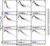 |
Fig. 2 Light curves in u- to H-band of 26 SE SNe with data obtained prior to tmax in at least one band. Each filtered light curve is normalized to peak brightness and aligned to tmax estimated from the best fit of Eq. (1)(colored solid lines) to the observed photometry. Shown below each light-curve panel are the residuals of the light-curve fits. Objects are color-coded based on their subtype: SNe IIb are green, SNe Ib are blue, SNe Ic are red, and SNe Ic-BL are magenta. |
Plotted in Fig. 1 is the best fit of Eq. (1)to the r-band light curve of SN 2006T. The fit clearly provides a smooth representation of the light curve, and this is particularly the case when the rise-to and subsequent fall-from peak brightness is well sampled. Some of the objects in the CSP-I sample were observed slightly prior to tmax. In these cases the denominator of Eq. (1)was set to unity in order to ensure convergence of the fit. In addition, for SNe observed only around peak and for less than seven epochs, the functional fits to the light curve was limited to a single Gaussian. Shown in Fig. 2 are the best fits of Eq. (1)to the optical and NIR light curves of the CSP-I SE SN sample. Overall, regardless of filter, the light curves are characterized by a single Gaussian-shape peak, followed a few weeks past tmax by a linear declining phase. In Sect. 3 we only consider those SE SNe whose light-curve data begin before or just at maximum brightness at least in one band (26 events).
3.2. Light-curve peak epochs
An important parameter computed from the light-curve fitting described in Sect. 3.1 is tmax. Estimates of tmax for the filtered light curve of each SN with pre-maximum follow-up observations are reported in Table 2. Plotted in Fig. 3 is tmax for each observed passband [normalized to t(r)max: tmax−t(r)max] versus wavelength, where the effective wavelength of each CSP-I passband is indicated with a solid vertical line. In the top panel, the data are plotted individually for each SN, while in the bottom panel all of the data are combined into one figure.
Each SN reaches tmax first in the u band, and subsequently peaks in red optical passbands sequentially with increasing wavelength from the B to i bands. Close inspection of Fig. 3 indicates that the NIR passbands peak after the optical passbands, but the J- and/or H-band light curves often reach tmax simultaneously or even prior to t(Y)max. This holds independent of the SE SN subtype. The dispersion around the general trend of later peak epochs at longer wavelength is larger in the NIR.
The behavior of the blue passbands peaking prior to the red passbands confirms a trend noted in the SDSS-II SE SN sample (Taddia et al. 2015), and is a reflection of the rapid cooling of the SN ejecta around maximum (see Sect. 5.3). Compared to the SDSS-II SE SN sample, the CSP-I SE SN sample extends the observed wavelength coverage out through 1.8 microns. This is highlighted by the solid red line in the bottom panel of Fig. 3, corresponding to a low-order polynomial fit to the data, as compared to the solid blue line, which is a similar fit to the SDSS-II SN survey’s SE SN sample. The function is steep at optical wavelengths and turns over to being nearly flat at NIR wavelengths. In the caption of Fig. 3 we report the expression of this best polynomial fit. The extended fit allows for the prediction (with ≈± 1.4 d uncertainty) of tmax for SE SNe with light curves observed prior to maximum in the red passbands but that lack pre-maximum observations in the blue passbands. In Table 2 a star indicates any peak epochs derived using this method.
3.3. Light-curve decline-rate parameter Δm15
A common light-curve decline-rate parameter to characterize the light curves of thermonuclear Type Ia supernovae (SNe Ia) is Δm15 (Phillips 1993). By definition Δm15 is the difference in the brightness of a SN between peak and 15 days later. In the case of SNe Ia, the luminosity-decline rate is known to correlate with luminosity in the sense that smaller Δm15 values correspond to more luminous objects (Phillips 1993).
The light-curve parameter Δm15 is readily computed from the light-curve fits presented in Sect. 3.1, and the resulting values are listed in Table 3 and plotted in Fig. 4. Plotted individually in the top panel of Fig. 4 is Δm15 versus wavelength for 24 SE SNe (those with observed maxima in the light curves and with at least 15 days of observations after peak), where the effective wavelengths of the CSP-I passbands are indicated with vertical lines. Clearly passbands with bluer effective wavelengths exhibit higher Δm15 values, implying faster declining light curves. This trend holds irrespective of SE SN subtype, with an average Δm15(u) ≈ 2.0 mag and an average Δm15(H) ≈ 0.4 mag. Plotted in the bottom panel of Fig. 4 are all of the SNe along with a low-order polynomial fit to the data (solid red line, reported in the caption). Examination of the distributions of Δm15 values yields no significant differences between the different SE SN subtypes, which is in agreement with previous studies by Drout et al. (2011) and Taddia et al. (2015).
Optical- and NIR-band epochs of peak maximum (JD−2 450 000).
3.4. Light curves beyond a month past maximum
Beginning around three weeks past maximum, the light-curve evolution of SE SNe begins to show significant diversity (see Fig. 2). This motivated us to consider the alternative light-curve parameter Δm40. Measurements of Δm40 from the r-band light curves are found to show standard deviation of 0.31 and 0.50 mag for the SN Ib and SN Ic sub-samples, and 0.07 mag for the SN IIb sub-sample. The fact that the light curves of SNe IIb are more uniform than those of the other SE SN subtypes was recently noted by Lyman et al. (2016), and this applies to all of the optical band light curves. The average Δm40 values are similar among the three different subtypes (1.5–1.7 mag in r band).
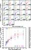 |
Fig. 3 Top panel: epoch of maximum light (relative to tmax in the r band) as a function of wavelength, where the effective wavelengths of the CSP-I passbands are indicated with solid vertical lines. Included here are 22 objects whose light curves cover the r-band maximum. The SE SN subtype of each object is indicated by the color of its name with green, blue, red, and magenta corresponding to Type IIb, Type Ib, Type Ic, and Type Ic-BL, respectively. Bluer optical bands peak prior to redder optical bands, while in the NIR, tmax is nearly coeval amongst the Y, J, and H passbands. Bottom panel: same as in the top panel, but here all the SNe are plotted together. The red solid line corresponds to a low-order polynomial fit, with the associated fit uncertainty of ≈1.4 days indicated by dashed red lines. The functional form of the polynomial fit is: tmax(λ)−tmax(r) = −8.0285λ2 + 23.234λ−11.476, with time in days and λ in μm. The solid blue line corresponds to the polynomial fit obtained from the SDSS-II SE SN sample (Taddia et al. 2015). |
Further inspection of the r-band light-curve fits in Fig. 2 indicates that the majority of objects with observations up to at least +40 d follow a similar linear decline rate of ≈2 mag per one hundred days at late epochs. The post maximum linear decline phase marks the time when energy deposition is dominated by the 56Co →56Fe decay chain. In principle, steeper slopes in the light curves correspond to events with higher gamma-rays escape fractions due to higher explosion energy to ejecta mass ratios and/or to higher degrees of 56Ni mixing (defined as the fraction of the total ejecta mass enclosed in the maximum radius reached by radioactive 56Ni). SNe IIb, Ib, and Ic exhibit rather uniform slopes quantified by 0.016–0.021 mag d-1, 0.014–0.018 mag d-1, and 0.017–0.027 mag d-1, respectively (see Fig. 5). These values are also consistent with the slopes measured in the other optical light curves. Comparing the late phase decline rates of our sample to that of the 56Co to 56Fe decay chain shows differences of ≈50%, suggesting that a significant fraction of gamma rays are not deposited into the SN ejecta. We will return to this issue in Sect. 7. In comparison, the r-band decline rate of normal SNe Ia is slower with a value of ≈0.014 mag d-1 (e.g., Stritzinger et al. 2002; Lair et al. 2006; Leloudas et al. 2009).
As evident from Fig. 2, the light curves of Type Ic SN 2005em evolve very rapidly over the SN’s post maximum decline phase. Indeed this object appears similar to a sub-class of fast evolving Type Ic objects that includes the well-studied SN 1994I (see, e.g., Clocchiatti et al. 2011).
In Fig. 5 we plot the late-time linear decay slope (parameter m in Eq. (1)) for those SNe with observations extending out to +40 d past V- and r-band maximum versus Δm15 in the same bands. This figure suggests a trend in the sense that objects characterized by faster decline rates in the two weeks after peak are also characterized by steeper slopes at later phases. This trend is also present in the i band (albeit less striking), whereas it is less clear whether it is present in bluer bands and in the NIR bands, where we have less late-time data. A possible interpretation of this trend is provided in Sect. 5. Finally, we note for comparison as indicated in the top panel of Fig. 5 that SNe Ia do not follow the same behavior in the V band.
3.5. Light-curve templates
Armed with the light-curve fits presented in Sect. 3.1, we proceed to construct template light curves covering the assortment of passbands used to observe SNe by the CSP-I. The resulting template light curves are plotted in Fig. 6. Templates were constructed by taking the average of the fits to the observed light curves, while the associated uncertainty is defined by the standard deviation of these fits.
The fit to the light curves that we used to build the templates are normalized to peak luminosity, so the templates show small dispersion around peak. After ≈+20 d the uncertainties of the templates become more significant given the large variety of decline rates that characterize the light curves (see Sect. 3.3) and the small sample size. Clearly the templates are broader in the red bands compared to the blue bands around maximum brightness.
Optical and NIR band Δm15 values.
With the r-band template light curve in hand, t(r)max is estimated for seven objects whose maximum was not entirely observed in the optical and/or NIR passbands. Estimates of t(r)max were obtained by fitting the r-band template (in the range between − 5 d and + 30 d) to the observed light curves, and the best estimates of t(r)max are indicated in Table 2 with a double star. We allow fits to the template from −5 d, as in some cases (e.g., SN 2009dp) the light curve around peak was poorly observed and the first detection may actually have occurred before peak.
The best fits are shown in the central panel of Fig. 6. An uncertainty of 1.5 days is adopted for all tmax values inferred from the template light-curve fits. For these seven objects, tmax in the other bands were then determined using the relation shown in Fig. 3. The r-band template is used to establish tmax in the bands without maximum coverage as r-band maximum occurs relatively late compared to the other optical passbands. Furthermore, for several objects their r-band light curves exhibit smaller scatter compared to the NIR light curves. The light curve templates are electronically3 available and can be used to constrain the phase and magnitude of peak for SE SNe observed after peak, as demonstrated in our analysis for several objects, and can also be used to aid in the photometric classification of SE SNe.
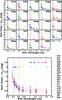 |
Fig. 4 Top panel: light-curve decline-rate parameter, Δm15, plotted as a function of wavelength where the effective wavelengths of the CSP passbands are indicated by vertical lines. At optical wavelengths the blue bands exhibit larger Δm15 values than the red bands, while in the NIR Δm15 is similar among the different bands. Bottom panel: same as in the top panel but with all SNe plotted in one panel, along with a low-order polynomial fit (solid red line) and its associated 1σ uncertainty (≈0.2 mag; dashed red line). The functional form of the polynomial fit is given by: Δm15(λ) = −11.88λ5 + 63.74λ4−134.17λ3 + 138.81λ2−71.00λ + 15.00. Here λ is in units of μm and Δm15 in units of magnitude. Shown in blue is a polynomial fit obtained from the same analysis of the SDSS-II SE SN sample (Taddia et al. 2015). |
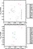 |
Fig. 5 Late-time linear decay slope in V and r band versus Δm15 for the CSP-I SE SNe with both their peak luminosity covered and their last observation being >+40 d days post maximum. Faster declining light curves (higher Δm15) tend to decline faster at late phases. Objects with both large uncertainties on the slope and on Δm15 are excluded from the figure. SN IIb, Ib, Ic, and Ic-BL are represented in green, blue, red, and magenta, respectively. SN 2005em is not included and falls far from the correlation due to its large late-time slope. With gray points we represent the results for the SNe Ia fit by Contardo (2001), which do not show any clear trend. |
4. Absolute magnitude light curves
Absolute magnitudes are computed from all apparent magnitudes corrected for reddening (see Sect. 2 and Table 1) and adopting the distances to their hosts given in Table 1 to set the absolute flux scale. The resulting absolute magnitude light curves are plotted in Fig. 7, and the peak absolute magnitude for each filtered light curve is reported in Table 5. The majority of objects (16 objects out of 22 in r band) reach peak absolute magnitudes ranging between − 17 mag and − 18 mag. The Type Ic-BL SN 2009ca is a significant outlier, reaching a maximum brightness Mr ≈ −20 mag, while the other Type Ic-BL in the sample, SN 2009bb, only lies at the bright end of the normal luminosity distribution of the sample.
To display the distribution of luminosities amongst SN IIb, SN Ib, and normal SN Ic subtypes, shown in Fig. 8 are the cumulative distribution functions (CDFs) of the peak absolute magnitudes for each of the CSP-I passbands. The CDFs for the SNe Ib and SNe Ic are consistent with those obtained from the SDSS-II SN Ib/c sample (Taddia et al. 2015). Inspection of the CDFs reveals no significant difference amongst the different subtypes. Indeed, a Kolmogorov–Smirnov (K–S) test reveals p-values > 0.05 in all but the Y band, where the comparison between SNe Ib and SNe Ic indicates p = 0.02 with SNe Ic being more luminous on average. The average peak absolute magnitudes for each subtype are reported in Table 5 and indicated by dashed vertical lines in Fig. 8.
In Table 5, next to the absolute-magnitude peak averages, we also report the associated dispersions for each band and each SE SN subtype. These are obtained from the standard deviations of the peak magnitudes. For instance, the dispersion of the r-band peak magnitudes are 0.54/0.60/0.21 mag for SNe IIb, Ib, and Ic, respectively. We investigated if these dispersions are mainly intrinsic or if they are mostly associated with uncertainties in the adopted distance and extinction. First, for each object we computed the uncertainty in the peak absolute magnitude, which is reported next to each peak magnitude in Table 5. These uncertainties are also reported as dotted lines in the cumulative distribution plots in Fig. 8, next to each peak magnitude value. The uncertainty of the peak of the absolute magnitudes was obtained by summing in quadrature the uncertainties associated with (i) the inferred peak apparent magnitude (see Table 4); (ii) the extinction; and (iii) the distance (see Table 1). We found, for example, that the r-band peak magnitudes extend from −17.38 to −17.91 mag for SNe Ic (so there are 0.53 mag between the faintest and the brightest object of the SN Ic sample), but when we consider the uncertainty in their peak magnitudes, their confidence intervals do not completely overlap only in the region between −17.53 and −17.59 mag. This implies that accounting for the uncertainty of the extinction and on the distance might reduce the observed difference among SN Ic peaks to a very tiny intrinsic difference. However, for SNe Ib and IIb the range where their peak r-band magnitude confidence intervals do not completely overlap is rather wide, ranging between −17.69 and −16.44 mag, and between −18.10 and −16.69 mag, respectively. Therefore, the dispersion in their peak luminosities is not only driven by the uncertainties of the distance and of the extinction, but reflects an intrinsic difference.
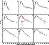 |
Fig. 6 SE SN light-curve templates. The templates were constructed by averaging the light-curve fits plotted in Fig. 2. The templates are represented by solid lines, their uncertainties by dashed lines. The r-band template light curve was used to estimate t(r)max for seven objects having follow-up observations beginning past peak (see central panel). Depending on their subtype, that is, IIb, Ib, Ic, and Ic-BL, these objects are represented in green, blue, red, and magenta, respectively. |
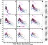 |
Fig. 7 Absolute magnitude uBgVriYJH-band light curves of the full CSP-I SE SN sample. SN IIb, Ib, Ic, and Ic-BL are represented in green, blue, red, and magenta, respectively. |
We now turn to the absolute peak magnitudes as a function of wavelength as plotted in Fig. 9. Strikingly, within the visual-wavelength region the peak luminosities are found to be dependent on the wavelength in the sense that red passbands tend to exhibit lower peak absolute magnitudes than the blue bands. Moving out to the NIR wavelengths the peak magnitudes continue to follow a trend of reaching lower values, though these values appear to be insensitive to the exact wavelength interval contained between ≈1.1 to 1.8 μm. Figure 9 suggests that the flux (in erg s-1 Å-1) at the effective wavelength of each passband and at the time of maximum in each specific band is higher at shorter effective wavelength. We note that since the peak magnitudes are measured at different epochs it is not a spectral energy distribution of the SN shown in the figure.
To end this section, in Fig. 10 we plot the peak absolute magnitudes of our SE SN sample versus the light-curve decline rate parameter Δm15 (see Sect. 3.3). Inspection of these parameters reveals mostly scatter plots in the various passbands. However, in the B band (and possibly also in the u band) the SNe IIb and SNe Ib exhibit a correlation between the two quantities in the sense that the more luminous objects tend to have broader light curves. A Spearman correlation test between the two quantities in the B band reveals a highly significant correlation with a p-value of 0.034. On the contrary, the correlation is not statistically significant in the u band. The correlation in B band is reminiscent of the well-known luminosity decline-rate relation of thermonuclear SNe Ia (Phillips 1993). This trend was not found in the bolometric light-curve analysis presented by Prentice et al. (2016) or in the ugriz light curves of the SDSS SNe Ib/c studied in Taddia et al. (2015). It is possible this correlation obtained from the CSP-I sample is due to the detailed treatment of host reddening (see Stritzinger et al. 2018b), which has a significant impact on the inferred peak absolute B-band magnitude. However, the accuracy of the CSP-I data themselves compared to that found in the literature may also be a significant contributing factor.
5. Bolometric properties
5.1. Spectral energy distributions
To capitalize on the extended wavelength range covered by the CSP-I observations, spectral energy distributions (SEDs) are constructed ranging from the u (320 nm) band redward to the H (1800 nm) band. Building a complete set of SEDs for each SN first requires the interpolation of each filtered light curve. Interpolation is accomplished with Gaussian process spline functions (see Stritzinger et al. 2018a), enabling measurements of both the optical and NIR flux at common epochs. Next, the magnitudes are corrected for dust extinction using reddening values computed by Stritzinger et al. (2018b). The extinction-corrected magnitudes are then converted to specific fluxes at the effective wavelength of each filter.
Peak optical and NIR apparent magnitudes.
Peak absolute magnitudes in the optical and NIR bands.
Unfortunately it was not possible to obtain complete light-curve coverage for some of the objects in the u and/or NIR passbands. In the u band this is typically due to a combination of low intrinsic brightness and fast evolution of the light curve, while at NIR wavelengths, gaps in follow-up are largely due to limitations of observational resources. To account for gaps in the u-band post-maximum follow-up, we resort to extrapolation when necessary. Specifically, a constant u−B color computed from photometry typically obtained after +15 d was adopted, and when combined with the B-band light curve, provides an accurate extrapolation of the u-band flux. If u-band photometry is completely missing, we make use of bolometric corrections (see below). Constructing SEDs that encompass some measure of the flux blue-wards of the atmospheric cutoff, we extrapolate from the wavelengths covered by the u band to zero flux at 2000 Å. This has been shown to provide a reasonable approximation of the flux in this wavelength region based on UV observations of a literature-based SE SN sample (Lyman et al. 2014). For SNe lacking NIR follow-up observations, we resort to extrapolation based on black-body (BB) fits to the optical-band SEDs, and the corresponding Rayleigh-Jeans tail accounts for flux red-ward of H band for the entire sample. By the end of this process, each SN has a set of SEDs with conservative corrections accounting for missing observations and flux emitted at the wavelength regions extending beyond those covered by the CSP-I passbands.
For the SNe with complete coverage between u and H band, the contribution to the total UVOIR flux in the UV (λ ≤ 3900 Å), optical (OPT; 3900 Å <λ< 9000 Å), and NIR (λ> 9000 Å) passbands can be determined as a function of phase. Doing so for the best observed objects provides the information shown in Fig. 11, which expresses the fraction of flux from these wavelength regions as a function of t(r)max. The fraction of flux in the optical always dominates, with the UV flux being non-negligible prior to t(r)max and the NIR flux becoming increasingly important after t(r)max. These findings are similar to those shown by Lyman et al. (2014), where slightly different wavelength ranges are considered.
The UV corrections obtained from extrapolation to zero flux at 2000 Å consist of ≈10% of the total flux around peak, whereas the mid- and far-IR corrections consist of only ≈3% of the total flux at similar epochs. At +20 d after peak the UV correction fraction drops to ≈3%, while the mid- to far-IR corrections rise to ≈5%.
5.2. UVOIR bolometric light curves
To produce a UVOIR light curve for a given SN, its time-series of SEDs are integrated over wavelength, and then the resulting total flux is placed on the absolute flux scale through the multiplication of the factor 4 , where DL is the luminosity distance to the host galaxy. In the case of those objects without any u-band photometry, we resort to constructing the UVOIR light curve by making use of the g-band photometry, the g−i color, and the bolometric corrections presented by Lyman et al. (2014). Through the comparison between the UVOIR light curves produced via the integration of SEDs and by the use of bolometric corrections, both techniques are found to provide fully consistent results over all epochs, in line with the precision discussed by Lyman et al. (2014, their Appendix B). The obtained UVOIR light curves of the CSP-I SE SN sample are plotted in the top panel of Fig. 12 and made available online on the Pasadena-based CSP-I webpage4. The associated uncertainties of the UVOIR luminosities are dominated by the error of the distance (ΔL/L ≈ 2ΔD/D), which is on the order of 7% (see the errors on the distances in Table 1). The majority of objects reach peak luminosities ranging between 1–10 × 1042 erg s-1. SN 2009ca is an outlier with Lmax ≈ 4 × 1043 erg s-1.
Each UVOIR light curve was fit with Eq. (1)and the results are over-plotted in Fig. 12 (top panel) as colored solid lines. This provides parameters characterizing the shape of these light curves, namely the epoch of bolometric peak [t(bol)max], the corresponding luminosity [L(bol)max], the decline-rate parameter [Δm15(bol)], and the slope of the linear decaying phase.
We find a correlation between Δm15(bol) and the late time slope (for the objects with at least one bolometric estimate +40 d after t(r)max). This is consistent with the same trend observed in the V and r bands, and it is shown in Fig. 13 (top-panel). This correlation might be explained in terms of the ratio between energy and ejecta mass. SE SNe with larger EK/Mej ratios will be less effective in trapping gamma-rays, and therefore will show steeper slopes at late times (see the parameter T0 in Wheeler et al. 2015). At early epochs, a larger EK/Mej ratio implies a shorter diffusion time and thus a narrower light curve, and therefore a larger Δm15(bol). However, when we check if the objects with broader (narrower) light curves and shallower (steeper) decay rates are also those with lower (higher) EK/Mej ratios (as computed in Sect. 6) this is not always the case.
The correlation between Δm15(bol) and M(bol)max is not as clear as is found for the B band (see bottom panel of Fig. 13). Finally, excluding the SN Ic-BL objects, there is no statistically significant difference between the peak luminosities of the various SE SN subtypes. The bolometric parameters discussed in this section are reported in Table 6.
5.3. Black-body fits: temperature, photospheric radius, and color-velocity (Vc) evolution
Byproducts of fitting BB functions to the SEDs of the CSP-I SE SN sample are estimates of the BB temperature ( ) and the “photospheric” radius (
 ) of the emitting region. Estimates of these parameters determined from BB fits to the gVri-band flux points are plotted in the middle and bottom panel of Fig. 12. The evolution of for the sample is remarkably uniform and this holds across subtypes and exhibits a scatter of no more than ≈1000 K beyond +5 d. Prior to maximum the scatter is more pronounced with found to reach peak values extending from 6000 K up to 10 000 K. By a couple of months past maximum is found to be 5500 ± 1000 K, irrespective of the SE SN subtype. We emphasize that the computed values are not sensitively dependent on the exact passbands used in the fit, for example, if g band is included or not, and this is a reflection of the photosphere cooling over time.
However, the uniformity of the temperatures is at least partly a consequence of the assumption on the host-extinction corrections, which were derived assuming intrinsic colors for each SN subtypes (Stritzinger et al. 2018b). This basically means that the extinction corrections to some degree minimize the temperature dispersion within each sub-class.
The is found to increase in all objects, reaching a maximum value around 15 days past r-band maximum. After the turnover it follows a slow decline. Typical values of the radius at tmax are 0.6−2.4 × 1015 cm, consistent with results obtained for the SDSS-II SE SN sample (Taddia et al. 2015).
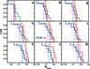 |
Fig. 8 Absolute peak magnitude distributions for the uBgVriYJH-bands for the CSP-I SE SN sample. SNe IIb, Ib, and Ic are represented in green, blue, and red, respectively. The two SNe Ic-BL in our sample have been omitted. The average peak magnitudes of each subtype are marked by vertical dashed lines. The uncertainty of each peak value is marked by a dotted line. |
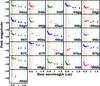 |
Fig. 9 Peak absolute magnitudes plotted as a function of wavelength, where the effective wavelengths of the CSP-I passbands are indicated with vertical lines. At optical wavelengths, SE SNe generally show higher values in the blue passbands compared to the red passbands. Among the NIR passbands, SE SNe exhibit similar peak absolute magnitudes and the values at NIR wavelengths are lower than those in the optical. SNe IIb, Ib, Ic, and Ic-BL are represented in green, blue, red, and magenta, respectively. |
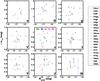 |
Fig. 10 Peak absolute magnitudes versus Δm15 for the CSP-I SE SN sample in nine different passbands. SNe IIb, Ib, Ic, and Ic-BL are represented in green, blue, red, and magenta, respectively. |
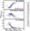 |
Fig. 11 Contribution of the UV, optical, and IR fluxes to the bolometric flux of 20 CSP-I SE SNe with at least one epoch of observations spanning from u to H band. The optical flux dominates at all epochs, the NIR flux becomes important at late time, whereas the UV fraction is non-negligible only before maximum. SNe IIb, Ib, Ic, and Ic-BL are represented in green, blue, red, and magenta, respectively. |
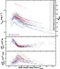 |
Fig. 12 Plotted in the top panel are the bolometric light curves of 33 SE SNe. Each of the light curves was fit with the function presented in Eq. (1), and the best fit is shown by solid colored lines. Shown in the middle and bottom panels is the temporal evolution of |
With BB fits to each object’s set of SEDs in hand, it is straightforward to compute the color velocity (Vc) parameter and its gradient ( ) (Piro & Morozova 2014, see their Eq. (1)). The color velocity corresponds to the velocity of the material at . Piro & Morozova argue that high values of Vc and are indicative of ejecta material characterized by large density gradients as expected in the outer regions of the expanding ejecta. Conversely, low values of Vc and are indicative of material located in deeper regions of the ejecta that are expanding more slowly than in the outer layers near the surface. Plotted in Fig. 14 (top panel) is Vc versus days past explosion (hereafter texp, see Sect. 6.1). Clearly Vc is highest in the moments following the explosion and subsequently decreases over time. We notice that a peak in the Vc profiles occurs at ≈30 d, and this is due to the evolution of RBB, which also peaks around that epoch. By texp = + 20 d a little over half of the sample’s Vc value drop below ≈10 000 km s-1, while by texp = +60 d, Vc extends from as much as ≈4000 km s-1 down to as little as ≈1500 km s-1. Each of the SE SN subtypes are represented at the high end of the Vc distribution (e.g., SN Ic 2004fe, SN Ib 2006ep, and SN IIb 2009Z), while at the low end only two SNe Ic (2005aw, 2009dp) are present. Indeed, most of the SNe Ic in the sample appear to exhibit relatively high Vc values at the time of explosion. SNe Ic also show the highest values of , again with the exceptions of SN 2005aw and SN 2009dp. We plotted in the bottom panel of Fig. 14. Examination of the low end of the Vc distribution reveals the presence of several SNe IIb and SNe Ib with low Vc, such as SN 2006T, SN 2006lc, SN 2007Y, SN 2008aq, SN 2007C, SN 2007kj, and SN 2008gc. We note that Folatelli et al. (2014b) recently identified a family of SNe Ib/IIb that exhibit flat and low (≈4000 and 8000 km s-1) helium velocity evolution extending from before maximum light to past +30 d.
6. Modeling
We now turn to modeling the CSP-I SE SN bolometric light curves in order to estimate key explosion parameters including: the explosion energy (EK), the ejecta mass (Mej), the 56Ni mass, and the degree of 56Ni mixing in the ejecta. In what follows, these parameters are computed by both semi-analytical modeling (where 56Ni mixing is not accounted for) and more sophisticated hydrodynamical modeling. To perform this modeling requires an estimation to the explosion epoch and a measure of the ejecta velocity.
6.1. Explosion epochs
To accurately fit the synthetic light curve to the UVOIR light curve of each SN requires an estimate of its explosion epoch. Depending on the discovery details and the subsequent follow-up observations, several techniques are utilized to estimate the explosion epochs for the SNe in our sample. In cases when the last non-detection and discovery epoch are less than four days apart, a mean value is adopted. If such limits are not available, the explosion epoch is computed from a power-law (PL) fit to the photospheric radius for all epochs prior to t(r)max. The adopted PL follows as rph(t) ∝ (t−texpl)0.78 (see Piro & Nakar 2013), and it is used to predict an explosion epoch constrained to occur between the last non-detection and the discovery epoch. For objects with poor pre-explosion limits and limited early-time coverage their explosion epochs are extrapolated assuming a typical r-band rise time (tr). Here we adopt tr = 13 ± 3 days for SNe Ic and tr = 22 ± 3 days for SNe Ib and SNe IIb (cf. Taddia et al. 2015). Relying on these assumptions enables reasonable explosion epoch estimates for objects with well-constrained values of t(r)max (see Table 2). Our best inferred explosion epochs are reported in Table 7, which also provides the method used to estimate them, and details regarding the last non-detection, discovery, and confirmation epochs. The application of these various methods to fit for the explosion epoch is demonstrated in Fig. 15.
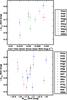 |
Fig. 13 The decline parameter Δm15 computed for the bolometric light curves versus the late-time linear decay slope (top panel) and the peak bolometric magnitude (bottom panel). A possible correlation is observed in the first case, which might be explained by a range of values of the EK/Mej ratio (see Sect. 5). SNe IIb, Ib, Ic, and Ic-BL are represented in green, blue, red, and magenta, respectively. |
Bolometric light-curve parameters.
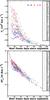 |
Fig. 14 Color velocity (Vc) plotted as a function of days past explosion (top-panel), and color velocity’s gradient (bottom panel). |
To summarize, we adopted the average between last non-detection and discovery in four cases (method “L” in Table 7, where we had good constraints); we used the fit to the black-body radius in seven cases (method “R” in Table 7); we adopted an average rise time based on the spectroscopic class (method “T”) for 19 SNe; finally, we adopted explosion epochs from the literature in three cases (see notes a, b, and c in Table 7). We decided to infer the explosion epoch following these methods and to propagate its uncertainty instead of leaving it as a free parameter in the modeling of the bolometric light curves (see Sect. 6.3), because the explosion epoch parameter is strongly degenerate with the ratio of energy and ejecta mass and with the amount of 56Ni mass intended to be estimated.
JD and magnitude of last-non detection, discovery, and confirmation epochs and estimated explosion epoch for 33 CSP-I SE SNe.
6.2. Photospheric and ejecta velocities
Another key input parameter required to fit semi-analytical and hydrodynamical models to the UVOIR light curves is the photospheric velocity (vph). Measured as the Doppler velocity at maximum absorption, vph serves as an important constraint on the ratio between the EK and Mej. In the following, vph values are adopted from Doppler velocity measurements of the Fe iiλ5169 feature (cf. Branch et al. 2002; Richardson et al. 2006), which are presented in a companion paper by Holmbo et al. (in prep.). Plotted in Fig. 16 are the resulting vph values versus days relative to explosion epoch, with the associated uncertainties being on the order of 500 km s-1. Inspection of the vph measurements reveals similar values for each of the SE SN subtypes over the same epochs, and the evolution of vph is found to be well-represented by a PL function characterized by an index α = −0.41 (dashed line in Fig. 16). As expected, the Type Ic-BL SN 2009bb and SN 2009ca exhibit significantly higher vph values, several thousand of km s-1 higher than the rest of the sample over the same epochs. These two objects are omitted when computing the PL fit.
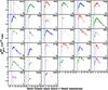 |
Fig. 15 Illustration of the different techniques used to estimate the explosion epochs for the CSP-I SE SN sample. The photospheric radius as a function of days since r-band maximum is shown for each SN in each sub-panel. The epoch of r-band maximum is marked by a black dotted line, the last non-detection epoch is indicated by a thick, blue dashed line, and the discovery epoch is indicated by a thick, red dashed line. The pre-peak fit to the radius with a PL is indicated by a green solid line and the corresponding explosion epoch estimate is indicated with a green dashed line. The explosion epochs derived by assuming a specific rise time for each subtype are marked by a black dashed line. The best explosion epoch estimate obtained for each object is marked by a cyan solid line and its corresponding uncertainties with cyan dashed lines. The method used to obtain the explosion epoch are indicated in each sub-panel. The letter L corresponds to the use of pre-discovery limits, R corresponds to the use of a PL radius fit, T assumes a rise time; Tl marks the case of assuming the last non-detection epoch as the explosion epoch (as the assumed rise time would have implied a too early explosion as compared to the last non detection), and Td marks when the assumed rise time and discovery epoch are used to determine the uncertainty of the explosion epoch as it occurred close to the inferred explosion. Finally, a,b,c are estimates obtained from the literature (see Table 7). Each SN is color-coded so that SNe IIb, Ib, Ic, and Ic-BL are green, blue, red, and magenta, respectively. |
For the semi-analytic models we use the value of vph at peak luminosity [vph(tmax)] to constrain EK/Mej. These are computed by fitting a PL to the measured Fe iiλ5169 velocities for each SN and taking the value of the best fit at the peak epoch. Assuming the ejecta are spherical and with constant density the EK to Mej ratio is given by the expression: 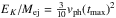 (Wheeler et al. 2015).
Following Dessart et al. (2016, see their Sect. 5.3), an alternative approach to constrain the EK to Mej ratio is to determine the quantity  . In the case of helium rich SNe IIb and SNe Ib, the Doppler velocity of the He iλ5875 feature can provide a measure of Vm, while for SNe Ic the O iλ7774 feature is appropriate.
 |
Fig. 16 Top panel: evolution of the Doppler velocity at maximum absorption of the Fe iiλ5169 feature for 32 SE SNe. SNe IIb, Ib, Ic, and Ic-BL are represented in green, blue, red, and magenta, respectively. The SNe IIb, Ib, and Ic follow a similar evolution that can be represented by a PL function. The SNe Ic-BL are found to exhibit higher velocities at all epochs and have therefore been excluded from the PL fit (dashed line). Middle panel: velocity evolution of He iλ5876 for SNe IIb (green) and Ib (blue), fitted by a PL. Bottom panel: velocity evolution of O iλ7772 for SNe Ic (red) and Ic-BL (magenta), fitted by a PL. |
Doppler velocity measurements of these lines and other spectral features are presented in the companion CSP-I SE SN spectroscopy paper (Holmbo et al., in prep.). The corresponding He i and O i Doppler velocity measurements are plotted in the central and bottom panels of Fig. 16, respectively. The Doppler velocity evolution of these features is well fit by PL functions (dashed lines) characterized by index values of −0.21 (He i) and −0.18 (O i). When fitting the Fe ii, He i, and O i line velocities, we adopted a unique PL index for all the objects. This is done to more robustly fit the velocity profiles of the events with a low number of spectra. However, we have also tested if this index is well suited for the events with numerous spectra. In particular, in the case of SN 2006T, we found that fitting its velocity profile with the PL index as a free parameter gives a similar index (− 0.35 instead of − 0.41) and an interpolated velocity at the maximum epoch, which differs from the one derived with fixed index by merely ≈290 km s-1, that is, below the typical velocity uncertainty. For each SN, the He i (if Type IIb or Ib) or O i (if Type Ic) velocities are fit with the proper PL in order to derive the velocity at peak, and this is used to directly estimate Vm.
6.3. Progenitor parameters from Arnett’s equations
We first proceed to fit the bolometric light curves with an Arnett (1982) model, assuming the explosion epochs given in Table 7 and . This provides a measure of EK, Mej, and the 56Ni mass. The specific function to model the UVOIR luminosity is presented by Cano (2013, see their Eq. (1)). In the process of computing a light-curve model, a constant opacity κ = 0.07 cm2 g-1 is adopted, as was done in Cano (2013) and Taddia et al. (2015), and implied by the models of SN 1998bw presented by Chugai (2000). The fit is done only including luminosity measurements obtained prior to 60 days past the explosion epoch, when the SNe are in their photospheric phase. When computing the best-fit Arnett model, the gamma-ray escaping fraction was also considered using the method of Wheeler et al. (2015) and recently utilized by Karamehmetoglu et al. (2017).
Plotted in Fig. 17 are the UVOIR light curves of the CSP-I SE SN sample along with the best-fit analytical and hydrodynamical models (see below). Also plotted within the panel of each UVOIR light curve is a sub-panel displaying the measured vph values, and the adopted vph(tmax) value at the epoch of t(r)max is also indicated in each sub-panel. The resulting key explosion parameters obtained from the two methods are reported in Table 8, along with averaged values for each SE SN subtype. The error on the 56Ni mass is dominated by the error on the SN distance, but also includes the error associated with the explosion epoch estimate as well as the fit uncertainty. The errors on EK and Mej are largely dominated by the uncertainty of the explosion epoch. SNe IIb, Ib, and Ic show typical ejecta masses of 4.3(2.0) M⊙, 3.8(2.1) M⊙, and 2.1(1.0) M⊙, respectively; kinetic energies are found to be 1.3(0.6) × 1051 erg, 1.4(0.9) × 1051 erg, and 1.2(0.7) × 1051 erg, respectively; 56Ni masses are 0.15(0.07) M⊙, 0.14(0.09) M⊙, and 0.13(0.04) M⊙, respectively.
Plotted in Fig. 18 is a clear correlation between EK and Mej as found from the Arnett model, and there are possible correlations between these two parameters and the 56Ni mass. Similar results were found by Lyman et al. (2016). In Fig. 19, the cumulative distributions of the three parameters for the three main classes indicates that the only difference between SNe IIb, Ib, and Ic is that SNe Ic possibly have lower ejecta masses. A K–S test reveals the difference is significant (p-value = 0.007) for the comparison between SNe Ic and SNe IIb.
 |
Fig. 17 Semi-analytic and hydrodynamical models of the bolometric light curves and vph profiles of 33 CSP-I SE SNe. Dashed black lines represents to the best-fit Arnett bolometric model and the vph(tmax) velocity derived from Fe iiλ5169 lines. Solid black lines represents the best-fit hydrodynamical model and corresponding velocity evolution. |
Explosion parameters for 33 CSP-I SE SNe from the semi-analytic and hydrodynamical modeling of their bolometric light curves.
A major limitation in applying semi-analytic modeling techniques to SE SN UVOIR light curves is the assumption of a constant opacity, denoted κ. Dessart et al. (2016) showed how different assumptions on the value of κ can lead to different results for the best progenitor parameters, and that ultimately, the assumption of constant opacity is quite poor for SE SNe. In the context of the semi-analytic model, we explore how our results vary depending on the value adopted for κ. Instead of κ = 0.07 cm2 g-1, we perform Arnett fits with κ = 0.05, 0.10, and 0.15 cm2 g-1. In Fig. 20 the best fit parameters for the four different values of opacity are reported. It is evident how larger opacities can lead to lower values of both EK and Mej, without modifying the 56Ni mass. Looking at the average for each subtype, a change in opacity from κ = 0.05 cm2 g-1 to κ = 0.15 cm2 g-1 reduces EK and the ejecta mass by 67% for each SE SN subtype.
We also explore how our results are affected by using vph values obtained from the Fe ii line velocities compared to using Vm as derived from the He i and O i line velocities at peak. Assuming a constant opacity (i.e., κ = 0.07 cm2 g-1), this comparison reveals nearly identical 56Ni masses, very similar ejecta masses, while the energies differ, especially for the SNe Ic. The comparisons between the parameters derived with the two different assumptions on the velocity and using the Arnett model is shown in Fig. 21.
6.4. Progenitor parameters from hydrodynamical models
Estimates for the explosion parameters are also obtained through hydrodynamical models compared to the UVOIR light-curve and velocity evolution of each SN. To do so a grid of light-curve models and their associated velocity evolution is computed using one-dimensional Lagrangian local thermal equilibrium (LTE) radiation hydrodynamics calculation (Bersten et al. 2011), based on hydrogen deficient He-core stars (see Bersten et al. 2012, for more details). The grid of models is constructed by exploding a series of relatively compact (R< 3 R⊙) structures with Helium-core masses of 3.3 M⊙ (He3.3), 4 M⊙ (He4), 5 M⊙ (He5), 6 M⊙ (He6), and 8 M⊙ (He8). These pre-supernova models originate from stellar evolutionary calculations of single stars with zero-age-main-sequence masses of 12 M⊙, 15 M⊙, 18 M⊙, 20 M⊙, and 25 M⊙, respectively (Nomoto & Hashimoto 1988).
 |
Fig. 18 Correlations between the explosion parameters obtained from the Arnett models of 33 CSP-I SE SNe. SNe IIb, Ib, Ic, and Ic-BL are represented in green, blue, red, and magenta, respectively. |
To explode the initial hydrostatic configuration some energy is artificially injected near the center of the pre-supernova star, yielding the formation of a shock wave that propagates through and unbinds the stars. As is well known, most of the light-curve evolution in SE SNe is powered mainly by the energy produced by radioactive decay because the explosion energy itself is rapidly degraded due to the compactness of the progenitor. To treat the γ photons produced from radioactive decay we assume gray transfer with a γ-ray mean opacity of κγ = 0.06 Ye cm2 g-1 (see Swartz et al. 1995), where Ye is the electron to baryon fraction. We allow for any distribution of 56Ni inside the ejecta. In this analysis, we have assumed a linear 56Ni distribution with a maximum value in the central region, and extended inside the configuration out to a specific fraction of the total mass (defined as the mixing parameter; see Table 8). Our calculations enable us to self-consistently determine the propagation of the shock wave through the star, and follow it through breakout and its subsequent light-curve emission out to late phases. However, we do not calculate the 56Ni production as a consequence of the explosive nucleosynthesis. We simply assume it as a free parameter of the model to be estimated by fitting the bolometric light curve.
In order to find an optimal model for each object in our sample, we have calculated an extensive grid of models for different values of the explosion energy, 56Ni mass, and distribution for a given pre-supernova structure. The grid of hydro models was then compared to our UVOIR light curves and the photospheric velocity evolution estimated from Fe ii λ5169 (see Sect. 6.2). This allowed us to select models that simultaneously reproduce both observables thus reducing the known degeneracy between Mej and Eexp. We note that the light-curve peak is extremely sensitive to the amount of 56Ni produced during the explosion, while the width around the main peak is primarily sensitive to Mej and Eexp. If very early observations are available, that is, before the rise to the main peak, then it is possible to estimate the size of the progenitor via hydrodynamical modeling. However, even with the excellent coverage of the CSP-I sample, the early cooling phase of the light curves is missing in most of the objects with the possible exception of the Type IIb SN 2009K.
Best-fit-model light curves and velocity profiles are plotted on top of the corresponding SN data in Fig. 17. The corresponding model parameters are listed in Table 8. Overall, the results are rather similar to those obtained with the Arnett models. Figure 22 shows the cumulative distributions for the parameters of the three main subtypes, revealing very similar ejecta mass, energy, and 56Ni mass distributions. SNe IIb, Ib, and Ic have average ejecta masses of 2.9(1.3) M⊙, 3.2(1.3) M⊙, and 2.8(1.2) M⊙, respectively; kinetic energies are found to be 1.2(0.7) foe5, 1.6(0.9) foe, and 1.4(1.0) foe, respectively; and 56Ni masses are 0.16(0.07) M⊙, 0.14(0.09) M⊙, and 0.16(0.06) M⊙, respectively.
Interestingly, the average degree of 56Ni mixing, which is defined as the fraction of mass enclosed within the maximum radius of the 56Ni distribution, is found to be larger in SNe Ic compared to SNe IIb and Ib. Quantitatively, for the CSP-I sample of SNe Ic the mixing parameter is found to be 1.0 for all the objects except SNe 2006ir and 2005aw (the average is 0.95), as compared to 0.75 ± 0.18 and 0.83 ± 0.12 for the SNe IIb and Ib, respectively. All our SE SNe are found to have 56Ni mixed out to ≳45% of the ejecta mass.
It is important to note that the mixing parameter is extremely sensitive to the estimate of the explosion time, which in some cases is not tightly constrained. Another factor that can affect our results, in particular for SN Ic progenitors, is the initial progenitor star model. Helium stars were adopted for the initial configurations in our calculations, whereas SN Ic progenitors are thought to be largely stripped of their helium envelopes. We adopted helium-rich models since there are currently no helium-free structures available in the literature to use in our hydro calculations for SNe Ic bolometric light curves.
7. Discussion
Key explosion parameters for the SN sample were estimated using both semi-analytic and hydrodynamical modeling techniques. In our analysis we elected to include all of the objects not observed early enough to directly estimate their peak bolometric light curve. At the end of Table 8 we report the average EK, Mej, and 56Ni mass obtained from our modeling efforts when excluding these objects. We note that, if average explosion parameters are estimated using the entire CSP-I sample, consistent results are obtained (within the errors) compared to those obtained from just the best-observed subset. This is an encouraging finding and suggests our efforts to estimate the explosion epoch and the peak luminosity for poorly observed objects do provide for reasonable estimates on their explosion parameters.
We proceed to compare our semi-analytic results to those obtained from other SE SN samples in the literature, as well as to compare the parameters derived from the two different methods. Based on the results concerning these parameters, we discuss the implications for the nature of the SE SN progenitor stars.
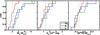 |
Fig. 19 Cumulative distributions (solid lines) of the explosion parameters obtained from the Arnett models of 31 CSP-I SE SNe (the two SNe Ic-BL are not included). SNe IIb, Ib, and Ic are represented in green, blue, and red, respectively. The average value of each distribution is marked by a vertical dashed line. |
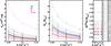 |
Fig. 20 Best explosion parameters (EK, Mej, M(56Ni)) from the Arnett models of 33 CSP-I SE SNe as a function of the opacity. SNe IIb, Ib, Ic, and Ic-BL are represented in green, blue, red, and magenta, respectively. Thick solid lines represent the average for each subtype. Larger opacities imply lower values of EK and Mej. For clarity, SN 2009ca is not shown in the M(56Ni) subpanel. |
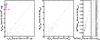 |
Fig. 21 Best explosion parameters (EK, Mej, M56Ni) from the Arnett models of 33 CSP-I SE SNe as computed using vph from Fe ii versus those computed using Vm from He i and O i as explained in Dessart et al. (2016). SNe IIb, Ib, Ic, and Ic-BL are represented in green, blue, red, and magenta, respectively. The dashed lines indicate when the parameters are identical with the two methods. Identical 56Ni masses are derived and very similar ejecta masses, whereas the energy obtained with the velocities from He i and O i are typically larger than those obtained with the Fe ii velocity, especially for SNe Ic. |
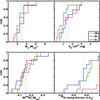 |
Fig. 22 Cumulative distributions (solid lines) of the explosion parameters obtained from the hydrodynamical models of 31 CSP-I SE SNe (the two SNe Ic-BL are not included). SNe IIb, Ib, and Ic are represented in green, blue, and red, respectively. The average value of each distribution is marked by a vertical dashed line. |
Comparison of the explosion parameters for different SE SN samples in the literature, from semi-analytic models.
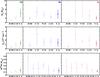 |
Fig. 23 Explosion and progenitor parameter comparisons among different works in the literature (R+06 = Richardson et al. 2006; D+1 = Drout et al. 2011; C 13 = Cano 2013; T+15 = Taddia et al. 2015; L+16 = Lyman et al. 2016; P+16 = Prentice et al. 2016; T. w. = this work), which include samples of SE SNe (IIb, Ib, Ic) and make use of semi-analytic models. |
7.1. Comparison with other samples in the literature
In Table 9 we present the average explosion and progenitor parameters for the different SE SN subtypes as derived from a number of samples in the literature. We compare these published results with our semi-analytic estimates, and the comparison is illustrated in Fig. 23. We stress that we are comparing works where the parameters were computed with similar models, and in particular the ejecta mass and the explosion energy parameters were derived based on almost identical assumptions regarding the adopted opacity (0.06–0.07 cm2 g-1). The only exceptions are the EK and Mej values derived by Richardson et al. (2006), who adopted κ ≃ 0.4 cm2 g-1.
The results of our UVOIR light-curve fits confirm relatively low values (2.1–4.3 M⊙) of the ejecta mass for SNe IIb, Ib, and Ic. Among the subtypes, we found SNe Ib and IIb to exhibit larger average ejecta mass than SNe Ic. However, within the uncertainty, these averages are still similar, as found for example by Lyman et al. (2016). Turning to the explosion energy, each of the subtypes exhibit values of EK = 1.2–1.4 × 1051 erg, which is entirely consistent with estimates of previous works. The average 56Ni mass for the three main subtypes ranges between 0.13 and 0.15 M⊙. These values are somewhat lower than those found from the study of the untargeted SDSS-II SN survey, though this discrepancy is due to their sample containing more distant objects (see Taddia et al. 2015). In summary, the comparison between the parameter estimates from the Arnett models indicates no significant differences among the subtypes, with the possible exception of the ejecta masses of SNe Ic being lower than those of SNe IIb, at least in our work.
In Table 9 and in Fig. 23 we do not include a comparison for the SNe Ic-BL, since we only have two objects in our sample. However, we notice that, in agreement with other works in the literature, our SNe Ic-BL clearly exhibit higher values of EK and 56Ni compared to the other subtypes.
7.2. Comparison between hydrodynamical and semi-analytic models
One of the properties that we can derive with the hydrodynamical models is the degree of 56Ni mixing. This is not possible with Arnett’s model, where the radioactive material is assumed to be centrally located in the ejecta. The mixing parameter is important to estimate because a 56Ni distribution that reaches the outer ejecta can affect the light-curve shape, in particular on the rising part. In our models we found SNe Ic are more mixed than SNe Ib and IIb. All of the SE SNe are found to be affected by a large degree of 56Ni mixing. With the exception of one event, all the SNe Ic are found to be fully mixed. Studies on the mixing of 56Ni in core-collapse SN ejecta date back to SN 1987A (see Shigeyama & Nomoto 1990; Woosley & Weaver 1995, and references therein). Numerical modeling shows the possibility that low 56Ni mixing can imply the absence of He lines in the spectra despite the presence of He in the ejecta (e.g., Dessart et al. 2011). However, recently we have found evidence for significant mixing in the SNe Ic from studying the SDSS-II SE SN sample (Taddia et al. 2015). Recently, Cano et al. (2014) has also presented evidence for significant mixing from their analysis of the Type Ib SN 1999dn.
Upon comparison of the other key explosion parameters derived from the Arnett and hydrodynamical models, as shown in Fig. 24, we find that 56Ni masses, Mej, and EK are in good agreement, with the Arnett models providing slightly larger ejecta masses and kinetic energies for three objects. Dessart et al. (2016) have recently suggested that Arnett models can give very different light curves compared to those obtained from hydrodynamical models. This suggestion is inconsistent with our results and we conclude that adopting a mean opacity of κ = 0.07 cm2 g-1 provides reasonable results to be compared to the more sophisticated hydrodynamical modeling.
7.3. Implications for the progenitor systems of SE SNe
Stellar-evolution theory shows that single stars below a certain initial mass are unable to strip their outer envelopes, given that their line-driven winds are not strong enough to sustain large mass-loss rates for enough time (see, e.g., Smith 2014, for a recent review on the mass loss of massive stars). For relatively low initial-mass stars, to strip the outer hydrogen layers, and in the case of SNe Ic, also the helium envelopes, mass transfer to a companion star is required (see, e.g., Yoon et al. 2010). We can consider the ejecta-mass estimates of our SNe and interpret them by using stellar-evolution models in order to infer the nature of their progenitor stars. Following the approach by Lyman et al. (2016), we consider that single progenitor star models with initial masses above 20 M⊙, computed by the binary population and spectral synthesis (BPASS) code (Eldridge et al. 2008; Eldridge & Stanway 2009), cannot produce ejecta masses below a value of about five M⊙. However, binary models of less massive stars calculated with the same code can easily leave behind lower (<4 M⊙) H-poor ejecta masses when they explode. The left panel of Fig. 19 and the probability distribution functions (PDFs) in the top panel of Fig. 25 show that the Arnett models suggest our SE SNe have ejecta masses ≲6 M⊙. For SNe Ic the limit is even lower, with only a small probability of events having ejecta masses above ≈5 M⊙.
In order to build the probability distribution of the SN ejecta masses, we consider each ejecta mass estimate Mej and its associated error σ, and construct a Gaussian distribution centered around Mej, with standard deviation equal to σ, and a normalization equal to one divided by the number of event of each subclass. Finally, to obtain the final probability distribution, all of the Gaussian distributions were summed.
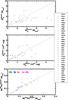 |
Fig. 24 Explosion and progenitor parameter comparisons between the hydrodynamical models and the semi-analytic models. |
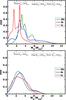 |
Fig. 25 Top panel: probability distribution function of the ejecta masses obtained from the Arnett models of 31 CSP-I SE SNe. SNe IIb, Ib, and Ic are represented in green, blue, and red, respectively. Bottom panel: probability distribution function of the ejecta masses obtained from the hydrodynamical models of 29 CSP-I SE SNe. |
In Lyman et al. (2016), the ejecta-mass distribution for SNe IIb and SNe Ib peaks at lower values compared to our distributions, favoring the binary scenario for the progenitors of these SNe. In our study, a scenario with a significant majority (92%) of helium-poor SNe coming from low-mass stars in binary systems still holds. To compute this 92%, we assumed Mej = 4.5 M⊙ from Lyman et al. as the upper limit to have low-mass binary progenitors with initial masses <20 M⊙. If we instead assume Mej = 5.5 M⊙ from Lyman et al. as the threshold to have single massive progenitors (with initial masses >28 M⊙), only 1.6% of the SNe Ic possibly come from massive single stars, or from massive binary progenitors with initial masses >20 M⊙. In the case of helium-rich SNe, a non-negligible fraction (SNe IIb ≈ 19% and SNe Ib ≈ 21%) might come from massive binaries or massive single stars. These values are higher than those found by Lyman et al..
However, we have to keep in mind that our ejecta mass estimates from Arnett’s models are strongly dependent on the assumption regarding the opacity. As clearly shown in the central panel of Fig. 20, the ejecta masses of the most massive SE SNe would drop from ≈6 M⊙ to ≈5 M⊙ and from ≈5 M⊙ to ≈4 M⊙ if instead of κ = 0.07 cm2 g-1 we adopt κ = 0.10 cm2 g-1. On the other hand, a lower opacity (κ = 0.05 cm2 g-1) would increase the number of SE SNe with ejecta masses above ≈5 M⊙, and thus they could possibly arise from single stars. Overall, the ejecta masses derived from the Arnett models for our SE SNe still favor the binary scenario for the majority of their progenitors, though we do not exclude the existence of a small fraction of single massive progenitors. We also note that the discussion above does not consider models with fast rotating SN progenitors, which can make a 40 M⊙ initial-mass star produce only ≈5.2 M⊙ of ejecta Dessart et al. (see 2017).
In order to overcome the degeneracy inherent to the assumption of constant opacity in the ejecta-mass estimates, we turn for guidance to our hydrodynamical models. To do so, assuming an uncertainty of ±1 M⊙ for our ejecta mass estimate from the hydrodynamical models, we can draw the probability density functions for the ejecta masses that are shown in the bottom panel of Fig. 25. In this case the SNe Ic are more similar to SNe IIb and Ib, which in turn have lower masses than those obtained with the application of Arnett’s model. The probability of having single massive stars as the progenitors of these SE SNe is rather low for all the subtypes, in good agreement with the PDF obtained by Lyman et al. (2016). Finally, the large degree of mixing found for SNe Ic suggests (see also Taddia et al. 2015) that the lack of helium is real for this SE SN subtype, and it is not due to the helium not being ionized by radioactive material (see Dessart et al. 2011).
8. Conclusions
We presented the analysis of a sample of 34 SE SNe from the CSP-I. Our main findings concerning their light-curve shapes are:
-
SE SNe show similar light-curve propertiesamong the three main subtypes, in particular similar Δm15 and peakabsolute magnitudes (typically − 18 <Mmax(r) < −17 mag).
-
Δm15is found to correlate with the slope of the light curve during its linear decay. This can be explained in terms of the large spread of explosion energy over ejecta mass (EK/Mej), with larger values corresponding to larger Δm15 and steeper late-time slopes.
-
A possible correlation between Δm15(B) and peak absolute B-band magnitude is found, reminiscent of a well-known trend followed by thermonuclear SNe Ia.
Our main findings concerning the progenitor properties based on bolometric modeling are:
-
From our hydrodynamical models, typical ejecta masses forSE SNe are found to be relatively small(1.1–6.2 M⊙) and thus incompatible with the majorityof events arising from massive single stars.
-
This result for the mass is similar when we consider the ejecta masses from the semi-analytic models, even though these are known to be affected by the assumptions regarding the constant value of the opacity. We found that assuming κ= 0.07 cm2 g-1 provides a good agreement between the results of the hydrodynamical models and those of the semi-analytical models. We also found that inferring the expansion velocity directly from Fe ii or via He i and O i for He-rich and He-poor SNe does not significantly alter the results on the ejecta mass.
-
SNe Ic tend to exhibit a larger degree of mixing among the various SE SN subtypes, suggesting that the lack of helium in their spectra corresponds to an actual lack of this element in the progenitors.
The template light curves can be downloaded in electronic format from the Pasadena-based CSP-I webpage: http://csp.obs.carnegiescience.edu/data/ and we point out to any potential users that the templates are on the CSP-I photometric system.
A foe is a unit of energy equivalent to 1051 erg.
Acknowledgments
We thank P. Hoeflich, P. A. Mazzali, and A. Piro for useful discussions. F. Taddia and J. Sollerman gratefully acknowledge support from the Knut and Alice Wallenberg Foundation. M. D. Stritzinger, C. Contreras, and E. Y. Hsiao acknowledge generous support provided by the Danish Agency for Science and Technology and Innovation realized through a Sapere Aude Level 2 grant and the Instrument-center for Danish Astrophysics (IDA). M. D. Stritzinger is supported by a research grant (13261) from VILLUM FONDEN. This material is based upon work supported by the US National Science Foundation (NSF) under grants AST–0306969, AST–0607438, and AST–1008343, AST–1613426, AST-1613455 and AST-1613472. A portion of the work presented here was done at the Aspen Center for Physics, which is supported by NSF grant PHY-1066293. This research has made use of the NASA/IPAC Extragalactic Database (NED), which is operated by the Jet Propulsion Laboratory, California Institute of Technology, under contract with the National Aeronautics and Space Administration.
References
- Anderson, J. P., Covarrubias, R. A., James, P. A., Hamuy, M., & Habergham, S. M. 2010, MNRAS, 407, 2660 [NASA ADS] [CrossRef] [Google Scholar]
- Anupama, G. C., Sahu, D. K., Deng, J., et al. 2005, ApJ, 2005, 631, L125 [Google Scholar]
- Arcavi, I., Gal-Yam, A., Yaron, O., et al. 2011, ApJ, 742, L18 [NASA ADS] [CrossRef] [Google Scholar]
- Arnett, W. D. 1982, ApJ, 253, 785 [NASA ADS] [CrossRef] [Google Scholar]
- Arnett, W. D., & Falk, S. W. 1976, ApJ, 210, 733 [NASA ADS] [CrossRef] [Google Scholar]
- Barbon, R., Buondi, V., Capperllaro, E., & Turatto, M. 1999, A&AS, 139, 531 [NASA ADS] [CrossRef] [EDP Sciences] [Google Scholar]
- Bersten, M. C., Benvenuto, O., & Hamuy, M. 2011, ApJ, 729, 61 [NASA ADS] [CrossRef] [Google Scholar]
- Bersten, M. C., Benvenuto, O. G., Nomoto, K., et al. 2012, ApJ, 757, 31 [NASA ADS] [CrossRef] [Google Scholar]
- Bersten, M. C., Tanaka, M., Tominaga, N., Benvenuto, O. G., & Nomoto, K. 2013, ApJ, 767, 143 [NASA ADS] [CrossRef] [Google Scholar]
- Bianco, F. B., Modjaz, M., Hicken, M., et al. 2014, ApJS, 213, 19 [NASA ADS] [CrossRef] [Google Scholar]
- Branch, D., Benetti, S., Kasen, D., et al. 2002, ApJ, 566, 1005 [NASA ADS] [CrossRef] [Google Scholar]
- Bufano, F., Pignata, G., Bersten, M., et al. 2014, MNRAS, 439, 1807 [NASA ADS] [CrossRef] [Google Scholar]
- Cano, Z. 2013, MNRAS, 434, 1098 [NASA ADS] [CrossRef] [Google Scholar]
- Cano, Z., Maeda, K., & Schulze, S. 2014, MNRAS, 438, 2924 [NASA ADS] [CrossRef] [Google Scholar]
- Cao, Y., Kasliwal, M. M., Arcavi, I., et al. 2013, ApJ, 775, L7 [NASA ADS] [CrossRef] [Google Scholar]
- Catchpole, R. M., Menzies, J. W., Monk, A. S., et al. 1987, MNRAS, 229, 15 [NASA ADS] [CrossRef] [Google Scholar]
- Chugai, N. N. 2000, Astron. Lett., 26, 797 [NASA ADS] [CrossRef] [Google Scholar]
- Clocchiatti, A., Suntzeff, N. B., Covarrubias, R., & Candia, P. 2011, AJ, 141, 163 [NASA ADS] [CrossRef] [Google Scholar]
- Contardo, G. 2011, Ph.D. Thesis, https://mediatum.ub.tum.de/doc/602863/602863.pdf [Google Scholar]
- Contardo, G., Leibundgut, B., & Vacca, W. D. 2000, A&A, 359, 876 [NASA ADS] [Google Scholar]
- Dessart, L., Hillier, D. J., Livne, E., et al. 2011, MNRAS, 414, 2985 [NASA ADS] [CrossRef] [Google Scholar]
- Dessart, L., Hillier, D. J., Woosley, S., et al. 2016, MNRAS, 458, 1618 [NASA ADS] [CrossRef] [Google Scholar]
- Dessart, L., John Hillier, D., Yoon, S.-C., Waldman, R., & Livne, E. 2017, A&A, 603, A51 [NASA ADS] [CrossRef] [EDP Sciences] [Google Scholar]
- Drout, M. R., Soderberg, A. M., Gal-Yam, A., et al. 2011, ApJ, 741, 97 [NASA ADS] [CrossRef] [Google Scholar]
- Eldridge, J. J., & Maund, J. R. 2016, MNRAS, 461, L117 [NASA ADS] [CrossRef] [Google Scholar]
- Eldridge, J. J., & Stanway, E. R. 2009, MNRAS, 400, 1019 [NASA ADS] [CrossRef] [Google Scholar]
- Eldridge, J. J., Izzard, R. G., & Tout, C. A. 2008, MNRAS, 384, 1109 [NASA ADS] [CrossRef] [Google Scholar]
- Eldridge, J. J., Fraser, M., Smartt, S. J., Maund, J. R., & Crockett, R. M. 2013, MNRAS, 436, 774 [NASA ADS] [CrossRef] [Google Scholar]
- Ensman, L., & Burrows, A. 1992, ApJ, 393, 742 [NASA ADS] [CrossRef] [Google Scholar]
- Ergon, M., Sollerman, J., Fraser, M., et al. 2014, A&A, 562, A17 [NASA ADS] [CrossRef] [EDP Sciences] [Google Scholar]
- Filippenko, A. V. 1997, ARA&A, 35, 309 [NASA ADS] [CrossRef] [Google Scholar]
- Filippenko, A. V., Matheson, T., & Ho, L. C. 1993, ApJ, 415, L103 [NASA ADS] [CrossRef] [Google Scholar]
- Filippenko, A. V., Matheson, T., & Barth, A. J. 1994, AJ, 108, 2220 [NASA ADS] [CrossRef] [Google Scholar]
- Filippenko, A. V., Barth, A. J., Matheson, T., et al. 1995, ApJ, 450, L11 [NASA ADS] [CrossRef] [Google Scholar]
- Fitzpatrick, E. L. 1999, PASP, 111, 63 [NASA ADS] [CrossRef] [Google Scholar]
- Folatelli, G., Contreras, C., Phillips, M. M., et al. 2006, ApJ, 641, 1039 [NASA ADS] [CrossRef] [Google Scholar]
- Folatelli, G., Bersten, M. C., Benvenuto, O. G., et al. 2014a, ApJ, 793, L22 [NASA ADS] [CrossRef] [Google Scholar]
- Folatelli, G., Bersten, M. C., Kuncarayakti, H., et al. 2014b, ApJ, 792, 7 [NASA ADS] [CrossRef] [Google Scholar]
- Folatelli, G., Van Dyk, S. D., Kuncarayakti, H., et al. 2016, ApJ, 825, L22 [NASA ADS] [CrossRef] [Google Scholar]
- Fox, O. D., Azalee Bostroem, K., Van Dyk, S. D., et al. 2014, ApJ, 790, 17 [NASA ADS] [CrossRef] [Google Scholar]
- Fremling, C., Sollerman, J., Taddia, F., et al. 2014, A&A, 565, A114 [NASA ADS] [CrossRef] [EDP Sciences] [Google Scholar]
- Galama, T. J., Vreeswijk, P. M., van Paradijs, J., et al. 1998, Nature, 395, 670 [NASA ADS] [CrossRef] [Google Scholar]
- Gal-Yam, A. 2016, ArXiv e-prints [arXiv:1611.09353] [Google Scholar]
- Hakobyan, A. A., Mamon, G. A., Petrosian, A. R., Kunth, D., & Turatto, M. 2009, A&A, 508, 1259 [NASA ADS] [CrossRef] [EDP Sciences] [Google Scholar]
- Hakobyan, A. A., Adibekyan, V. Z., Aramyan, L. S., et al. 2012, A&A, 544, A81 [NASA ADS] [CrossRef] [EDP Sciences] [Google Scholar]
- Hamuy, M., Folatelli, G., Morrell, N., et al. 2006, PASP, 118, 2 [NASA ADS] [CrossRef] [Google Scholar]
- Hsiao, E. Y., Conley, A., Howell, D. A., et al. 2007, ApJ, 663, 1187 [NASA ADS] [CrossRef] [Google Scholar]
- Jerkstrand, A., Ergon, M., Smartt, S. J., et al. 2015, A&A, 573, A12 [NASA ADS] [CrossRef] [EDP Sciences] [Google Scholar]
- Karamehmetoglu, E., Taddia, F., Sollerman, J., et al. 2017, A&A, 602, A93 [NASA ADS] [CrossRef] [EDP Sciences] [Google Scholar]
- Komatsu, E., Dunkley, J., Nolta, M. R., et al. 2009, ApJS, 180, 330 [NASA ADS] [CrossRef] [Google Scholar]
- Krisciunas, K., Contreras, C., Burns, C. B., et al. 2017, AJ, submitted [Google Scholar]
- Lair, J. C., Leising, M. D., Milne, P. A., & Williams, G. G. 2006, AJ, 132, 2024 [NASA ADS] [CrossRef] [Google Scholar]
- Leloudas, G., Stritzinger, M. D., Sollerman, J., et al. 2009, A&A, 505, 265 [NASA ADS] [CrossRef] [EDP Sciences] [Google Scholar]
- Leloudas, G., Gallazzi, A., Sollerman, J., et al. 2011, A&A, 530, A95 [NASA ADS] [CrossRef] [EDP Sciences] [Google Scholar]
- Liu, Y. Q., Modjaz, M., Bianco, F., et al. 2016, ApJ, 827, 90 [NASA ADS] [CrossRef] [Google Scholar]
- Lyman, J. D., Bersier, D., & James, P. A. 2014, MNRAS, 437, 3848 [NASA ADS] [CrossRef] [Google Scholar]
- Lyman, J. D., Bersier, D., James, P. A., et al. 2016, MNRAS, 457, 328 [NASA ADS] [CrossRef] [Google Scholar]
- Malesani, D., Fynbo, J. P. U., Hjorth, J., et al. 2009, ApJ, 692, L84 [NASA ADS] [CrossRef] [Google Scholar]
- Maund, J. R., Smartt, S. J., Kudritzki, R. P., Podsiadlowski, P., & Gilmore, G. F. 2004, Nature, 427, 129 [NASA ADS] [CrossRef] [PubMed] [Google Scholar]
- Mazzali, P. A., Valenti, S., Della Valle, M., et al. 2008, Science, 321, 1185 [NASA ADS] [CrossRef] [PubMed] [Google Scholar]
- Modjaz, M., Li, W., Butler, N., et al. 2009, ApJ, 702, 226 [NASA ADS] [CrossRef] [Google Scholar]
- Modjaz, M., Kewley, L., Bloom, J. S., et al. 2011, ApJ, 731, L4 [NASA ADS] [CrossRef] [Google Scholar]
- Modjaz, M., Blondin, S., Kirshner, R. P., et al. 2014, AJ, 147, 99 [NASA ADS] [CrossRef] [Google Scholar]
- Mould, J. R., Huchra, J. P., Freedman, W. L., et al. 2000, ApJ, 529, 786 [NASA ADS] [CrossRef] [Google Scholar]
- Nakar, E., & Piro, A. L. 2014, ApJ, 788, 193 [NASA ADS] [CrossRef] [Google Scholar]
- Nomoto, K., & Hashimoto, M. 1988, Phys. Rep., 163, 13 [NASA ADS] [CrossRef] [Google Scholar]
- Oates, S. R., Bayless, A. J., Stritzinger, M. D., et al. 2012, MNRAS, 424, 1297 [NASA ADS] [CrossRef] [Google Scholar]
- Patat, F., Cappellaro, E., Danziger, J., et al. 2001, ApJ, 555, 900 [NASA ADS] [CrossRef] [Google Scholar]
- Phillips, M. M. 1993, ApJ, 413, L105 [NASA ADS] [CrossRef] [Google Scholar]
- Phillips, M. M., Simon, J. D., Morrell, N., et al. 2013, ApJ, 779, 38 [NASA ADS] [CrossRef] [Google Scholar]
- Pignata, G., Stritzinger, M., Soderberg, A., et al. 2011, ApJ, 728, 14 [NASA ADS] [CrossRef] [Google Scholar]
- Piro, A. L. 2015, ApJ, 808, L51 [NASA ADS] [CrossRef] [Google Scholar]
- Piro, A. L., & Morozova, V. S. 2014, ApJ, 792, L11 [NASA ADS] [CrossRef] [Google Scholar]
- Piro, A. L., & Nakar, E. 2013, ApJ, 769, 67 [NASA ADS] [CrossRef] [Google Scholar]
- Prentice, S. J., & Mazzali, P. A. 2017, MNRAS, 469, 2672 [NASA ADS] [CrossRef] [Google Scholar]
- Prentice, S. J., Mazzali, P. A., Pian, E., et al. 2016, MNRAS, 458, 2973 [NASA ADS] [CrossRef] [Google Scholar]
- Richardson, D., Branch, D., & Baron, E. 2006, AJ, 131, 2233 [NASA ADS] [CrossRef] [Google Scholar]
- Riess, A. G., Macri, L., Casertano, S., et al. 2011, ApJ, 732, 129 [NASA ADS] [CrossRef] [Google Scholar]
- Roy, R., Sollerman, J., Silverman, J. M., et al. 2016, A&A, 596, A67 [NASA ADS] [CrossRef] [EDP Sciences] [Google Scholar]
- Sanders, N. E., Soderberg, A. M., Levesque, E. M., et al. 2012, ApJ, 758, 132 [NASA ADS] [CrossRef] [Google Scholar]
- Schlafly, E. F., & Finkbeiner, D. P. 2011, ApJ, 737, 103 [NASA ADS] [CrossRef] [Google Scholar]
- Schlegel, D. J., Finkbeiner, D. P., & Davis, M. 1998, ApJ, 500, 525 [NASA ADS] [CrossRef] [Google Scholar]
- Shigeyama, T., & Nomoto, K. 1990, ApJ, 360, 242 [NASA ADS] [CrossRef] [Google Scholar]
- Shivvers, I., Modjaz, M., Zheng, W., et al. 2017, PASP, 129, 054201 [NASA ADS] [CrossRef] [Google Scholar]
- Smith, N. 2014, ARA&A, 52, 487 [NASA ADS] [CrossRef] [MathSciNet] [Google Scholar]
- Smith, N., Li, W., Filippenko, A. V., & Chornock, R. 2011, MNRAS, 412, 1522 [NASA ADS] [CrossRef] [Google Scholar]
- Soderberg, A. M., Berger, E., Page, K. L., et al. 2008, Nature, 453, 469 [NASA ADS] [CrossRef] [PubMed] [Google Scholar]
- Stritzinger, M. D. 2005, Ph.D. Thesis, Technical University of Munich [Google Scholar]
- Stritzinger, M., Hamuy, M., Suntzeff, N. B., et al. 2002, AJ, 124, 2100 [NASA ADS] [CrossRef] [Google Scholar]
- Stritzinger, M., Mazzali, P., Phillips, M. M., et al. 2009, ApJ, 696, 713 [NASA ADS] [CrossRef] [Google Scholar]
- Stritzinger, M. D., Anderson, J. P., & Contreras, C., et al. 2018a, A&A, 609, A134 [NASA ADS] [CrossRef] [EDP Sciences] [Google Scholar]
- Stritzinger, M. D., Taddia, F., Burns, C. R., et al. 2018b, A&A, 609, A135 [NASA ADS] [CrossRef] [EDP Sciences] [Google Scholar]
- Swartz, D. A., Sutherland, P. G., & Harkness, R. P. 1995, ApJ, 446, 766 [NASA ADS] [CrossRef] [Google Scholar]
- Taddia, F., Sollerman, J., Leloudas, G., et al. 2015, A&A, 574, A60 [NASA ADS] [CrossRef] [EDP Sciences] [Google Scholar]
- Taddia, F., Fremling, C., Sollerman, J., et al. 2016, A&A, 592, A89 [NASA ADS] [CrossRef] [EDP Sciences] [Google Scholar]
- Taddia, F., Sollerman, J., Fremling, C., et al. 2018, A&A, 609, A106 [NASA ADS] [CrossRef] [EDP Sciences] [Google Scholar]
- Tominaga, N., Tanaka, M., Nomoto, K., et al. 2005, ApJ 633, L97 [NASA ADS] [CrossRef] [Google Scholar]
- Vacca, W. D., & Leibundgut, B. 1996, ApJ, 471, L37 [NASA ADS] [CrossRef] [Google Scholar]
- Valenti, S., Taubenberger, S., Pastorello, A., et al. 2012, ApJ, 749, L28 [NASA ADS] [CrossRef] [Google Scholar]
- Van Driel, W., Yoshida, S., Nakada, Y., et al. 1993, PASJ, 45, L59 [NASA ADS] [Google Scholar]
- Wheeler, J. C., Johnson, V., & Clocchiatti, A. 2015, MNRAS, 450, 1295 [NASA ADS] [CrossRef] [Google Scholar]
- Woosley, S. E., & Weaver, T. A. 1995, ApJS, 101, 181 [NASA ADS] [CrossRef] [Google Scholar]
- Woosley, S. E., Eastman, R. G., Weaver, T. A., & Pinto, P. A. 1994, ApJ, 429, 300 [NASA ADS] [CrossRef] [Google Scholar]
- Yoon, S.-C. 2015, PASA, 32, 15 [NASA ADS] [CrossRef] [Google Scholar]
- Yoon, S.-C., Woosley, S. E., & Langer, N. 2010, ApJ, 725, 940 [NASA ADS] [CrossRef] [Google Scholar]
All Tables
JD and magnitude of last-non detection, discovery, and confirmation epochs and estimated explosion epoch for 33 CSP-I SE SNe.
Explosion parameters for 33 CSP-I SE SNe from the semi-analytic and hydrodynamical modeling of their bolometric light curves.
Comparison of the explosion parameters for different SE SN samples in the literature, from semi-analytic models.
All Figures
|
Fig. 1 Best fit of Eq. (1)(black solid line) to the r-band light curve (triangles) of SN 2006T normalized to its peak brightness. The three components of the analytic fit are shown: blue for the exponential rise, green for the Gaussian peak, and red for the linear decay. The corresponding terms in Eq. (1)are color-coded accordingly. The residuals between the fit and the photometry are plotted in the bottom panel, and in this case they never exceed 0.03 mag. |
| In the text | |
|
Fig. 2 Light curves in u- to H-band of 26 SE SNe with data obtained prior to tmax in at least one band. Each filtered light curve is normalized to peak brightness and aligned to tmax estimated from the best fit of Eq. (1)(colored solid lines) to the observed photometry. Shown below each light-curve panel are the residuals of the light-curve fits. Objects are color-coded based on their subtype: SNe IIb are green, SNe Ib are blue, SNe Ic are red, and SNe Ic-BL are magenta. |
| In the text | |
|
Fig. 3 Top panel: epoch of maximum light (relative to tmax in the r band) as a function of wavelength, where the effective wavelengths of the CSP-I passbands are indicated with solid vertical lines. Included here are 22 objects whose light curves cover the r-band maximum. The SE SN subtype of each object is indicated by the color of its name with green, blue, red, and magenta corresponding to Type IIb, Type Ib, Type Ic, and Type Ic-BL, respectively. Bluer optical bands peak prior to redder optical bands, while in the NIR, tmax is nearly coeval amongst the Y, J, and H passbands. Bottom panel: same as in the top panel, but here all the SNe are plotted together. The red solid line corresponds to a low-order polynomial fit, with the associated fit uncertainty of ≈1.4 days indicated by dashed red lines. The functional form of the polynomial fit is: tmax(λ)−tmax(r) = −8.0285λ2 + 23.234λ−11.476, with time in days and λ in μm. The solid blue line corresponds to the polynomial fit obtained from the SDSS-II SE SN sample (Taddia et al. 2015). |
| In the text | |
|
Fig. 4 Top panel: light-curve decline-rate parameter, Δm15, plotted as a function of wavelength where the effective wavelengths of the CSP passbands are indicated by vertical lines. At optical wavelengths the blue bands exhibit larger Δm15 values than the red bands, while in the NIR Δm15 is similar among the different bands. Bottom panel: same as in the top panel but with all SNe plotted in one panel, along with a low-order polynomial fit (solid red line) and its associated 1σ uncertainty (≈0.2 mag; dashed red line). The functional form of the polynomial fit is given by: Δm15(λ) = −11.88λ5 + 63.74λ4−134.17λ3 + 138.81λ2−71.00λ + 15.00. Here λ is in units of μm and Δm15 in units of magnitude. Shown in blue is a polynomial fit obtained from the same analysis of the SDSS-II SE SN sample (Taddia et al. 2015). |
| In the text | |
|
Fig. 5 Late-time linear decay slope in V and r band versus Δm15 for the CSP-I SE SNe with both their peak luminosity covered and their last observation being >+40 d days post maximum. Faster declining light curves (higher Δm15) tend to decline faster at late phases. Objects with both large uncertainties on the slope and on Δm15 are excluded from the figure. SN IIb, Ib, Ic, and Ic-BL are represented in green, blue, red, and magenta, respectively. SN 2005em is not included and falls far from the correlation due to its large late-time slope. With gray points we represent the results for the SNe Ia fit by Contardo (2001), which do not show any clear trend. |
| In the text | |
|
Fig. 6 SE SN light-curve templates. The templates were constructed by averaging the light-curve fits plotted in Fig. 2. The templates are represented by solid lines, their uncertainties by dashed lines. The r-band template light curve was used to estimate t(r)max for seven objects having follow-up observations beginning past peak (see central panel). Depending on their subtype, that is, IIb, Ib, Ic, and Ic-BL, these objects are represented in green, blue, red, and magenta, respectively. |
| In the text | |
|
Fig. 7 Absolute magnitude uBgVriYJH-band light curves of the full CSP-I SE SN sample. SN IIb, Ib, Ic, and Ic-BL are represented in green, blue, red, and magenta, respectively. |
| In the text | |
|
Fig. 8 Absolute peak magnitude distributions for the uBgVriYJH-bands for the CSP-I SE SN sample. SNe IIb, Ib, and Ic are represented in green, blue, and red, respectively. The two SNe Ic-BL in our sample have been omitted. The average peak magnitudes of each subtype are marked by vertical dashed lines. The uncertainty of each peak value is marked by a dotted line. |
| In the text | |
|
Fig. 9 Peak absolute magnitudes plotted as a function of wavelength, where the effective wavelengths of the CSP-I passbands are indicated with vertical lines. At optical wavelengths, SE SNe generally show higher values in the blue passbands compared to the red passbands. Among the NIR passbands, SE SNe exhibit similar peak absolute magnitudes and the values at NIR wavelengths are lower than those in the optical. SNe IIb, Ib, Ic, and Ic-BL are represented in green, blue, red, and magenta, respectively. |
| In the text | |
|
Fig. 10 Peak absolute magnitudes versus Δm15 for the CSP-I SE SN sample in nine different passbands. SNe IIb, Ib, Ic, and Ic-BL are represented in green, blue, red, and magenta, respectively. |
| In the text | |
|
Fig. 11 Contribution of the UV, optical, and IR fluxes to the bolometric flux of 20 CSP-I SE SNe with at least one epoch of observations spanning from u to H band. The optical flux dominates at all epochs, the NIR flux becomes important at late time, whereas the UV fraction is non-negligible only before maximum. SNe IIb, Ib, Ic, and Ic-BL are represented in green, blue, red, and magenta, respectively. |
| In the text | |
|
Fig. 12 Plotted in the top panel are the bolometric light curves of 33 SE SNe. Each of the light curves was fit with the function presented in Eq. (1), and the best fit is shown by solid colored lines. Shown in the middle and bottom panels is the temporal evolution of |
| In the text | |
|
Fig. 13 The decline parameter Δm15 computed for the bolometric light curves versus the late-time linear decay slope (top panel) and the peak bolometric magnitude (bottom panel). A possible correlation is observed in the first case, which might be explained by a range of values of the EK/Mej ratio (see Sect. 5). SNe IIb, Ib, Ic, and Ic-BL are represented in green, blue, red, and magenta, respectively. |
| In the text | |
|
Fig. 14 Color velocity (Vc) plotted as a function of days past explosion (top-panel), and color velocity’s gradient (bottom panel). |
| In the text | |
|
Fig. 15 Illustration of the different techniques used to estimate the explosion epochs for the CSP-I SE SN sample. The photospheric radius as a function of days since r-band maximum is shown for each SN in each sub-panel. The epoch of r-band maximum is marked by a black dotted line, the last non-detection epoch is indicated by a thick, blue dashed line, and the discovery epoch is indicated by a thick, red dashed line. The pre-peak fit to the radius with a PL is indicated by a green solid line and the corresponding explosion epoch estimate is indicated with a green dashed line. The explosion epochs derived by assuming a specific rise time for each subtype are marked by a black dashed line. The best explosion epoch estimate obtained for each object is marked by a cyan solid line and its corresponding uncertainties with cyan dashed lines. The method used to obtain the explosion epoch are indicated in each sub-panel. The letter L corresponds to the use of pre-discovery limits, R corresponds to the use of a PL radius fit, T assumes a rise time; Tl marks the case of assuming the last non-detection epoch as the explosion epoch (as the assumed rise time would have implied a too early explosion as compared to the last non detection), and Td marks when the assumed rise time and discovery epoch are used to determine the uncertainty of the explosion epoch as it occurred close to the inferred explosion. Finally, a,b,c are estimates obtained from the literature (see Table 7). Each SN is color-coded so that SNe IIb, Ib, Ic, and Ic-BL are green, blue, red, and magenta, respectively. |
| In the text | |
|
Fig. 16 Top panel: evolution of the Doppler velocity at maximum absorption of the Fe iiλ5169 feature for 32 SE SNe. SNe IIb, Ib, Ic, and Ic-BL are represented in green, blue, red, and magenta, respectively. The SNe IIb, Ib, and Ic follow a similar evolution that can be represented by a PL function. The SNe Ic-BL are found to exhibit higher velocities at all epochs and have therefore been excluded from the PL fit (dashed line). Middle panel: velocity evolution of He iλ5876 for SNe IIb (green) and Ib (blue), fitted by a PL. Bottom panel: velocity evolution of O iλ7772 for SNe Ic (red) and Ic-BL (magenta), fitted by a PL. |
| In the text | |
|
Fig. 17 Semi-analytic and hydrodynamical models of the bolometric light curves and vph profiles of 33 CSP-I SE SNe. Dashed black lines represents to the best-fit Arnett bolometric model and the vph(tmax) velocity derived from Fe iiλ5169 lines. Solid black lines represents the best-fit hydrodynamical model and corresponding velocity evolution. |
| In the text | |
|
Fig. 18 Correlations between the explosion parameters obtained from the Arnett models of 33 CSP-I SE SNe. SNe IIb, Ib, Ic, and Ic-BL are represented in green, blue, red, and magenta, respectively. |
| In the text | |
|
Fig. 19 Cumulative distributions (solid lines) of the explosion parameters obtained from the Arnett models of 31 CSP-I SE SNe (the two SNe Ic-BL are not included). SNe IIb, Ib, and Ic are represented in green, blue, and red, respectively. The average value of each distribution is marked by a vertical dashed line. |
| In the text | |
|
Fig. 20 Best explosion parameters (EK, Mej, M(56Ni)) from the Arnett models of 33 CSP-I SE SNe as a function of the opacity. SNe IIb, Ib, Ic, and Ic-BL are represented in green, blue, red, and magenta, respectively. Thick solid lines represent the average for each subtype. Larger opacities imply lower values of EK and Mej. For clarity, SN 2009ca is not shown in the M(56Ni) subpanel. |
| In the text | |
|
Fig. 21 Best explosion parameters (EK, Mej, M56Ni) from the Arnett models of 33 CSP-I SE SNe as computed using vph from Fe ii versus those computed using Vm from He i and O i as explained in Dessart et al. (2016). SNe IIb, Ib, Ic, and Ic-BL are represented in green, blue, red, and magenta, respectively. The dashed lines indicate when the parameters are identical with the two methods. Identical 56Ni masses are derived and very similar ejecta masses, whereas the energy obtained with the velocities from He i and O i are typically larger than those obtained with the Fe ii velocity, especially for SNe Ic. |
| In the text | |
|
Fig. 22 Cumulative distributions (solid lines) of the explosion parameters obtained from the hydrodynamical models of 31 CSP-I SE SNe (the two SNe Ic-BL are not included). SNe IIb, Ib, and Ic are represented in green, blue, and red, respectively. The average value of each distribution is marked by a vertical dashed line. |
| In the text | |
|
Fig. 23 Explosion and progenitor parameter comparisons among different works in the literature (R+06 = Richardson et al. 2006; D+1 = Drout et al. 2011; C 13 = Cano 2013; T+15 = Taddia et al. 2015; L+16 = Lyman et al. 2016; P+16 = Prentice et al. 2016; T. w. = this work), which include samples of SE SNe (IIb, Ib, Ic) and make use of semi-analytic models. |
| In the text | |
|
Fig. 24 Explosion and progenitor parameter comparisons between the hydrodynamical models and the semi-analytic models. |
| In the text | |
|
Fig. 25 Top panel: probability distribution function of the ejecta masses obtained from the Arnett models of 31 CSP-I SE SNe. SNe IIb, Ib, and Ic are represented in green, blue, and red, respectively. Bottom panel: probability distribution function of the ejecta masses obtained from the hydrodynamical models of 29 CSP-I SE SNe. |
| In the text | |
Current usage metrics show cumulative count of Article Views (full-text article views including HTML views, PDF and ePub downloads, according to the available data) and Abstracts Views on Vision4Press platform.
Data correspond to usage on the plateform after 2015. The current usage metrics is available 48-96 hours after online publication and is updated daily on week days.
Initial download of the metrics may take a while.