| Issue |
A&A
Volume 606, October 2017
|
|
|---|---|---|
| Article Number | A95 | |
| Number of page(s) | 22 | |
| Section | Extragalactic astronomy | |
| DOI | https://doi.org/10.1051/0004-6361/201730669 | |
| Published online | 19 October 2017 | |
The spatially resolved stellar population and ionized gas properties in the merger LIRG NGC 2623
1 Instituto de Astrofísica de Andalucía (CSIC), PO Box 3004, 18080 Granada, Spain
e-mail: This email address is being protected from spambots. You need JavaScript enabled to view it.
2 Instituto de Astronomía, Universidad Nacional Autonóma de México, A.P. 70-264, 04510 México D.F., Mexico
3 Departamento de Física, Universidade Federal de Santa Catarina, PO Box 476, 88040-900 Florianópolis, SC, Brazil
4 Observatoire de Paris, GEPI, Observatoire de Paris, PSL Research University, CNRS, Univ. Paris Diderot, Sorbonne Paris Cité, Place Jules Janssen, 92195 Meudon, France
5 Department of Physics and Astronomy, University of Sheffield, Sheffield S3 7RH, UK
6 Centro de Astrobiología (INTA-CSIC), Carretera de Ajalvir, km 4, 28850 Torrejón de Ardoz, Madrid, Spain
7 Leibniz-Institut für Astrophysik Potsdam (AIP), An der Sternwarte 16, 14482 Potsdam, Germany
Received: 21 February 2017
Accepted: 5 June 2017
Abstract
We report on a detailed study of the stellar populations and ionized gas properties in the merger LIRG NGC 2623, analyzing optical integral field spectroscopy from the CALIFA survey and PMAS LArr, multiwavelength HST imaging, and OSIRIS narrow band Hα and [NII]λ6584 imaging. The spectra were processed with the starlight full spectral fitting code, and the results are compared with those for two early-stage merger LIRGs (IC 1623 W and NGC 6090), together with CALIFA Sbc/Sc galaxies. We find that NGC 2623 went through two periods of increased star formation (SF), a first and widespread episode, traced by intermediate-age stellar populations ISP (140 Myr–1.4 Gyr), and a second one, traced by young stellar populations YSP (<140 Myr), which is concentrated in the central regions (<1.4 kpc). Our results are in agreement with the epochs of the first peri-center passage (~200 Myr ago) and coalescence (<100 Myr ago) predicted by dynamical models, and with high-resolution merger simulations in the literature, consistent with NGC 2623 representing an evolved version of the early-stage mergers. Most ionized gas is concentrated within <2.8 kpc, where LINER-like ionization and high-velocity dispersion (~220 km s-1) are found, consistent with the previously reported outflow. As revealed by the highest-resolution OSIRIS and HST data, a collection of HII regions is also present in the plane of the galaxy, which explains the mixture of ionization mechanisms in this system. It is unlikely that the outflow in NGC 2623 will escape from the galaxy, given the low SFR intensity (~0.5 M⊙ yr-1 kpc-2), the fact that the outflow rate is three times lower than the current SFR, and the escape velocity in the central areas is higher than the outflow velocity.
Key words: galaxies: interactions / galaxies: evolution / galaxies: stellar content / galaxies: ISM / galaxies: star formation / techniques: spectroscopic
© ESO, 2017
1. Introduction
NGC 2623 (UGC 04509 = Arp 243; LIR = 3.56 × 10¹¹L⊙; e.g., Sanders et al. 2003) is an infrared luminous merger of galaxies located at a distance of 80 Mpc. It is an advanced merger, in stage IV (Veilleux et al. 2002), where the progenitor’s nuclei have already coalesced. The nucleus is extended and quite obscured in the ultraviolet (UV) and optical, and becomes very bright and point-like in infrared images. Moreover, this galaxy has two long and fairly symmetrical tidal tails, extending up to 20 kpc from the nucleus. The galaxy also shows a blue star forming region south of the main body (Evans et al. 2008). The near-infrared (NIR) surface brightness profile in the nuclear regions follows a r1 / 4 law, consistent with a system evolving into an elliptical galaxy (Wright et al. 1990; Rothberg & Joseph 2004). A substantial post-starburst population dominates in the circum-nuclear region of NGC 2623 (Joy & Harvey 1987; Armus et al. 1989; Liu & Kennicutt 1995; Shier et al. 1996), while a young nuclear starburst is also present (Bernloehr 1993; Shier et al. 1996). Evans et al. (2008) reported that the blue, UV-bright star forming region located 5 kpc south of the nucleus comprises ~100 star clusters with ages between 1 and 100 Myr. This region could be either part of a loop of material associated with the northern tidal tail, or nuclear tidal debris created during one of the final passages of the progenitor nuclei prior to their coalescence. The bulk of infrared luminosity comes from the obscured nuclear regions, and the off-nuclear starburst represents only 1% of the total star formation in NGC 2623. The ionization process in the nucleus of NGC 2623 is a combination of a dusty starburst and shock heating due to a starburst-related outflow (Lípari et al. 2004). The outflow has an opening angle θ = 100° ± 5° and reaches a distance of 3.2 kpc from the nucleus and a velocity of VOF = (−405 ± 35) km s-1. The nucleus hosts an obscured AGN, as determined from the hard X-ray spectrum (Maiolino et al. 2003) and the presence of the [NeV] 14.3 μm line (Evans et al. 2008; Petric et al. 2011), which contributes to 9% of the total nuclear radio emission, being energetically weak relative to the starburst population (Lonsdale et al. 1993).
In this paper, we aim to derive both the stellar population properties and the ionized gas properties of NGC 2623 in order to characterize in detail the merger-induced star formation and the ionization structure in the final stages of a major merger. Previous longslit studies in other merging (ultra)luminous infrared galaxies (U/LIRGs) have revealed that stellar populations of <2 Gyr have a widespread presence in these systems, while SP < 100 Myr are more significant in the nuclear regions of the galaxies (Rodríguez Zaurín et al. 2009). Although low-resolution merger simulations initially predicted that most star formation occurred in the central regions (Mihos & Hernquist 1996; Moreno et al. 2015), the new high-resolution models show that extended star formation is also present and important in the early phases of mergers (Teyssier et al. 2010; Hopkins et al. 2013; Renaud et al. 2015). In this sense, integral field spectroscopy (IFS) is a very promising technique, because it can provide relevant information to characterize the extent of star formation, and how/when it is produced. Extended star formation has also been observationally reported in many early-stage mergers, mainly in the form of widespread star clusters, most of which are located at the intersections between progenitors and/or tidal structures (Wang et al. 2004; Elmegreen et al. 2006; Smith et al. 2016), and through stellar population analysis relying on IFS (Cortijo-Ferrero et al. 2017; hereafter CF17). In fact, the results of the two early-stage merger LIRGs reported in CF17, IC 1623 W and NGC 6090, are compared throughout the paper with the merger LIRG NGC 2623. The advantage of NGC 2623 is that it is a more advanced system, in the merger stage, where a triggering of the star formation is expected to occur, but at the same time, it also keeps a fossil record in the stellar populations of previous star formation bursts (i.e., when it was at the early-stage merger phase). Therefore, NGC 2623 represents an interesting nearby LIRG to study the role that major mergers play in galaxy evolution using spatially resolved spectroscopy.
The layout of the paper is: Sect. 2 describes the observations and data reduction process. In Sect. 3 we apply the fossil record method to analyze the stellar continuum and derive the spatially resolved stellar population properties: stellar mass and stellar mass surface density, μ⋆; stellar extinction, AV; luminosity weighted mean age, ⟨ log age ⟩ L; and the contributions to luminosity and mass of young, intermediate, and old stellar populations. Section 4 presents results on the ionized gas emission, focussing on the morphology, nebular AV, the ionization conditions, and velocity dispersion. We discuss the results in Sect. 5, and Sect. 6 presents the conclusions.
Throughout the paper we assume a flat cosmology with ΩM = 0.272, ΩΛ = 0.728, and H0 = 70.4 k s-1 Mpc -1 (WMAP, seven-year results). For the NGC 2623 redshift (z = 0.018509), this results in a distance of 80.0 Mpc. At this distance 1′′ corresponds to 0.390 kpc.
2. Observations and data reduction
2.1. Integral field spectroscopy
The IFS data were taken with the Potsdam Multi-Aperture Spectrophotometer (PMAS) spectrograph (Roth et al. 2005) at the 3.5 m telescope of Calar Alto Observatory (CAHA). The nuclear region was observed in the Lens Array (LArr) mode, using a spatial magnification of 0.75′′/lens, covering a 12′′ × 12′′ field of view (FoV). The V300 grating was used, providing a 3.2 Å/pixel dispersion and covering a wavelength range 3700–7100 Å with a resolution of 7.1 Å full width at half maximum (FWHM), for a total exposure time of 2.5 h.
We also have data from the Calar Alto Integral Field Area (CALIFA) survey project (Sánchez et al. 2012), covering the main body of NGC 2623, and including virtually the entire extent of the system, except the outermost parts of the tidal tails. The CALIFA observations were conducted using PMAS in its PPAK (PMAS fibre PAcK) mode. Fibers in the PPAK bundle have a projected diameter on the sky of 2.7′′, covering 64′′ × 74′′ FoV. The spatial resolution of CALIFA data is FWHMPSF = 2.39 ± 0.26 arcsec (García-Benito et al. 2015). Observations were performed using the gratings V500 and V1200, with resolutions of 6.3 Å and 2.3 Å (FWHM), wavelength ranges of 3650–7500 Å and 3650–4840 Å, and total exposure times in each of 0.75 h and 1.5 h, respectively. Table A.1 summarizes the main characteristics of the IFS data.
2.1.1. LArr data reduction
The PMAS LArr data-reduction process is described in detail in CF17, which should be consulted for all the reduction details. Relative flux calibration was performed using the spectrophotometric standard star Feige 34. We have flux-recalibrated LArr data using HST (WFC435W, WFC555W) and SDSS (g, r-band) photometry, and have found an average accuracy of the spectrophotometric calibration of 13% ± 2% across the wavelength range covered by our data set.
2.1.2. CALIFA data reduction
The raw data were processed through an automatic pipeline, and the reduced data cubes made publicly available for the community (Husemann et al. 2013). In our case, we have analyzed the V500 combined with the V1200 data, to improve the signal in the blue side, and to reduce the effects of vignetting. The data analyzed in this paper were reduced using the CALIFA Pipeline version 1.5. The main reduction steps and properties of the reduced data are similar to the LArr ones, and are described in detail in Sánchez et al. (2012), based on version 1.2. A list of the differences and improvements with respect to this earlier version are presented in Husemann et al. (2013). The combined V1200 + V500 datacubes were processed as described in Cid Fernandes et al. (2013), and detailed in Sect. 3.1.
2.2. OSIRIS Tunable Filters data and reduction
We have taken Tunable Filter (TF) observations with OSIRIS at Gran Telescopio de Canarias (GTC) at the Roque de los Muchachos Observatory in La Palma. OSIRIS is an imager and spectrograph for the optical wavelength range, located in the Nasmyth-B focus of GTC. The OSIRIS observations were performed using TF imaging mode with a seeing ~0.9′′. A FoV of 260 × 520 arcsec square was covered with a spatial scale of 0.254′′/pixel. The red TF in scanning mode was used, covering Hα and [NII]λ6584 lines plus the adjacent continua. Filters were centered at λ0 = 6640, 6700, 6705, 6720, 6725, and 6760 Å, with a FWHM = 14 Å. These are the wavelength values at the optical center. The wavelength tuning is not uniform over the full FoV of OSIRIS. There is a progressive increasing shift to the blue of the central wavelength (λ0) as the distance from the optical center (r) increases. The wavelength (in Å) observed with the red TF relative to the optical center changes following the law reported by González et al. (2014):  (1)where r is the distance in arcminutes between the optical center and the CCD position at which we want to calculate the wavelength. In Fig. 3 we show the integrated CALIFA spectrum for NGC 2623, normalized at 5500 Å, in the Hα + [NII] region. In red we show the OSIRIS TF narrow-band filter bandpasses at the galaxy center, and in blue the position of the filters at the location of the star forming regions. We note how, due to the greater distance of the star forming regions from the optical center, the [NII] filter is displaced into the Hα region. Distances to the optical center above 2.2′ and below 1.3′ start to be affected by the shift in wavelength. In our case, only the edges of the tidal tails of NGC 2623 are affected, while the main body and the clumps in the north tidal tail (at 1.65′) are not. The object and the calibration star (Feige 34) were positioned at the same distance from the optical center and on the same CCD chip. We obtained three science frames per filter of 300 s exposure time each. The main information about TF data is summarized in the right column of Table A.1.
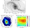 |
Fig. 1 Top panel: HST ACS F555W image of NGC 2623. The black rectangle indicates the FoV covered by the LArr IFS, while the black hexagon indicates PPaK FoV. Lower left panel: continuum flux at 5110 Å rest-frame (obtained by averaging the spectra in the range 5050–5170 Å), Fλ5110, for the CALIFA data. Lower right panel: Fλ5110 for LArr data. |
 |
Fig. 2 Left panel: HST F435W continuum image of NGC 2623, with the average continuum from CALIFA IFS superimposed using red contours. Several regions of the galaxy are labelled. Right panel: spectra from different regions extracted in circular apertures of 2′′ radius, in black the PPaK nuclear spectrum, in red the LArr nuclear spectrum, and in blue the spectrum from the cluster-rich region to the south of the nucleus. The spectra are normalized by the flux at 5500 Å, and an offset is applied to better visualize the differences. |
Summary of NGC 2623 IFS and TF narrow-band data.
The OSIRIS data were reduced using standard procedures for CCD imaging within the IRAF package. Due to the high dark level in the OSIRIS CCDs, a series of dark images with the same exposure time as the science data were taken. To remove the presence of several sky emission rings at the left edges of the image we developed a simple Python script that generated an artificial background map from the original images. Finally, a relative flux calibration was performed for each filter by comparing the aperture photometry of Feige 34 measured in OSIRIS data, with the theoretical value obtained from Oke (1990) calibrated spectra.
Once we had reduced all the science images, a mean continuum map was obtained by averaging the blue (6640 Å) and red (6760 Å) continua. Analogously, we obtained mean Hα+continuum and [NII]+continuum maps by averaging the 6700 Å and 6705 Å, and 6720 Å and 6725 Å filter data, respectively. By subtracting the mean continuum map from the latter images, we obtained the pure Hα and [NII] emission line maps shown in Sect. 4.
2.3. HST imaging
We downloaded from the Hubble Legacy Archive (HLA)1 multi-wavelength high-resolution images taken by the Hubble Space Telescope (HST) in several broad-band filters from far ultraviolet (FUV) to NIR: ACS F140LP, ACS F330W, ACS F435W, ACS F555W, ACS F814W, NICMOS F110W, and NICMOS F160W, covering the main body of NGC 2623. From these we derived the star-clusters photometry. All these images were retrieved in their pipeline reduced form, astrometrically corrected and aligned with North up, East left. Their characteristics are summarized in Table A.1.
2.4. An overview of the data
Figure 1 presents an overview of the data, indicating the FoV covered by LArr/PPaK over the HST/ACS F555W image, and the IFS continuum flux at 5110 Å. In the left panel of Fig. 2 we have highlighted, over the HST/ACS F435W image and PPaK continuum contours, some of the main regions of the galaxy. Their spectra are shown in the right panel. The nuclear spectra from LArr (black) and from CALIFA data (red) show good agreement in terms of the spectral continuum shape. They show prominent emission lines, as well as the high-order Balmer lines in absorption, indicating the coexistence of young and intermediate-age stellar populations. Dust extinction is important in the nucleus, as revealed by the continuum rise beyond 6000 Å (Sánchez Almeida et al. 2012). The spectrum of the star cluster region to the south is shown in blue, and is consistent with a stellar population with an age of a few Myr. Weak Hα and [NII] is also present.
3. Stellar populations
In this section we use the stellar continuum shape from the IFS to characterize the spatially resolved stellar population properties and constrain the star formation history (SFH) of NGC 2623. We have also performed an analysis based on the star clusters detected in HST images that is presented in Appendix A.
Moreover, in this Section we compare with the radial profiles of two control samples of 70 Sbc and 14 Sc CALIFA spirals (González Delgado et al. 2015), in the same mass range as NGC 2623.
3.1. Methodology
Our method of extracting stellar population information from the IFS data cubes is based on the full spectral synthesis approach.
For the CALIFA data cube, spectra suitable for a full spectral synthesis analysis of the stellar population content were extracted in a way that ensures a S/N ≥ 20 in a 90 Å wide region centered at 5635 Å (in the rest-frame). When individual spaxels did not meet this S/N threshold they were coadded into Voronoi zones (Cappellari & Copin 2003). Pre-processing steps also included spatial masking of foreground/background sources and very low S/N spaxels, rest-framing, and spectral resampling. The whole process took spectrophotometric errors (eλ) and bad pixel flags (bλ) into account. The spectra were then processed through PyCASSO (the Python CALIFA starlight Synthesis Organizer), producing the results discussed throughout this paper. For the LArr data, the process was similar, and is described in detail in CF17.
The results reported in this paper rely on the GM and CB model bases described in CF17. Basically, the GM base combines the granada models of González Delgado et al. (2005) with Vazdekis et al. (2010), and is based on the Salpeter initial mass function (IMF). The CB base is built from an update of the Bruzual & Charlot (2003) models, with a Chabrier IMF. Reddening is modelled as a foreground screen parametrized by AV (same reddening for all the SSP components) and following Calzetti et al. (2000) reddening law with RV = 4.5, which was derived from observations of starburst galaxies, and is found to be the most appropriate for interacting galaxies (Smith et al. 2016).
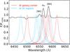 |
Fig. 3 Integrated CALIFA spectrum for NGC 2623 normalized at 5500 Å, in the Hα + [NII] region. The OSIRIS TF narrow-band filter bandpasses at the galaxy center are shown in red, while the positions of the filters at the location of the star forming regions (R1 to R4, see Sect. 4.7) are shown in blue. |
The quality of the spectral fits was examined using the  indicator (Cid Fernandes et al. 2013). We found median values of 6% and 5% for the CALIFA, and the LArr data, respectively. In the remainder of the paper, only the spaxels with
  are shown in the maps, and considered in the analysis.
The effects of the Voronoi binning are present in all panels, but they are more important in the maps of luminosity-independent properties, such as the AV map. This is because the maps of extensive properties (luminosity and mass) were “dezonified” by scaling the value at each xy spaxel by its fractional contribution to the total flux in a zone (z index in Eq. (2)). For example, for the stellar-mass surface density we have applied:  (2)where Mxy (Mz) is the stellar mass in a spaxel (zone), and Axy (Az) denotes the area in that spaxel (zone), and
  (3)where Fxy is the mean flux at 5635 ± 45 Å (for more details see Sect. 5.2 of Cid Fernandes et al. 2013). This operation was applied to luminosity and mass-related quantities, producing somewhat smoother images than obtained with wxyz = 1. However, intensive properties such as AV and mean age cannot be dezonified.
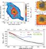 |
Fig. 4 Upper left: CALIFA map of the stellar mass surface density (μ⋆). The white dashed lines indicate the position of 1, 2, and 3 half-light radii (HLR); 1 HLR is equivalent to 2.8 kpc in physical distance. The contours correspond to the smoothed HST F555W image. Upper right: LArr map of stellar mass surface density. The color-scale is the same as for the CALIFA map. Below is presented a zoom of the CALIFA map in the nuclear region, to match the region covered by LArr map. Lower panel: radial profile of log μ⋆ as a function of the radial distance in HLR (lower horizontal axis) and kpc (upper horizontal axis), in red for LArr and black for CALIFA. The uncertainties, calculated as the standard error of the mean, are shaded in light red and gray, respectively. For comparison, the gray lines are the profiles from Sbc (solid) and Sc (dashed) spiral galaxies from CALIFA (González Delgado et al. 2015), with stellar masses similar to that of NGC 2623. We also include the profiles of the early-stage mergers IC 1623 W (blue), NGC 6090 NE (orange), and NGC 6090 SW (green). |
3.2. Results: Stellar mass and stellar-mass surface density
An important starlight output is the stellar mass, calculated from the stellar luminosity and taking into account the spatial variation of the mass-to-light ratio. The total stellar mass obtained by summing the mass of each zone is M⋆ = ∑ Mz = 5.4 × 10¹⁰M⊙. This is the mass locked in stars at the observation epoch. Counting also the mass returned by stars to the interstellar medium,  were involved in star formation. These results are for the GM base (Salpeter IMF). With the CB base (Chabrier IMF), we find
  and M⋆ = 2.4 × 10¹⁰M⊙2.
We note that we are not underestimating the stellar masses with the optical spectral synthesis, since they are similar to the dynamical mass estimated by Privon et al. (2013), Mdyn ≲ 6 × 10¹⁰M⊙, which represents a lower limit as it is derived using a numerical model of the interaction.
Figure 4 shows the stellar-mass surface density maps, μ⋆ (in M⊙ pc-2). The upper left panel is the full CALIFA map. The white dashed lines indicate the positions of 1, 2, and 3 half light radius (HLR)3. In this case, 1 HLR is equivalent to 2.8 kpc in physical distance, which is approximately in agreement with the half light radius measured by the CALIFA collaboration (10.3 arcsec = 4.0 kpc, Walcher et al. 2014) through the growth curve analysis in elliptical apertures of the SDSS r-band image.
The upper-right panels in Fig. 4 are the LArr map, and a zoom of the CALIFA map in the same region covered by LArr data. The 2D maps of the stellar population properties were azimuthally averaged to allow their radial variations to be studied using PyCASSO. Radial apertures of 0.1 HLR in width were used to extract the radial profiles. Expressing radial distances in units of HLR allows the profiles of NGC 2623 to be compared on a common metric with the control samples of Sbc and Sc galaxies. The lower panel shows the profile of log μ⋆ as a function of the radial distance in HLR, in red for LArr and black for CALIFA. The uncertainties are shaded in light red, and gray, and represent the standard error of the mean, calculated as the standard deviation divided by the square root of the number of points (N) in each radial distance bin. The differences in the uncertainties between the inner and outer regions are visually not strong, because the larger the radius, the larger N. In terms of dispersion (=standard deviation) we find that, with respect to the NGC 2623 center (N = 8, CALIFA data set, for consistency with above), the dispersion is a factor 2.2 larger at 0.5 HLR (N = 38), 2.9 larger at 1 HLR (N = 68), and 4 larger at 2 HLR (N = 128). For the LArr data, the dispersion is a factor 2.7 larger at 0.5 HLR (N = 59) than in the center (N = 8). For comparison, the gray lines are the profiles derived for Sbc (solid) and Sc (dashed) spiral galaxies from CALIFA (González Delgado et al. 2015; hereafter GD15), with masses consistent with that of NGC 2623. We also include the profiles of the early-stage mergers IC 1623 W (blue), NGC 6090 NE (orange) and NGC 6090 SW (green).
We find a negative trend of μ⋆ with distance using the CALIFA map: from log μ⋆ (M⊙ pc-2) ~ 3.8 in the nucleus itself to ~ 1.3 in the outer parts, at 3 HLR. The log μ⋆ values derived from the LArr data are 0.1–0.2 dex larger than those derived from the CALIFA data, but still within the dispersion. We find only minor differences in the stellar mass surface densities and the other stellar population properties (see Sects. 3.3 and 3.4) derived from CALIFA and LArr data sets, always within the uncertainties; they could be due to the different spatial and spectral resolution, and also to the effect of the age-AV degeneracy, which is the most difficult to break in dusty star forming galaxies such as NGC 2623.
The central stellar mass density of NGC 2623 is comparable to Sbc galaxies in the CALIFA sample. We have compared the inner (from 0 to 1 HLR) and outer (from 1 to 2 HLR) gradients of the stellar mass surface density (as defined in Eqs. (6) and (7) of GD15) in NGC 2623 and in the control spirals: Δin log μ⋆ = −1.22, −1.15, −0.99 for NGC 2623, Sbc, and Sc galaxies, respectively; and Δout log μ⋆ = −0.80, −0.64, −0.54 for NGC 2623, Sbc, and Sc galaxies, respectively. The stellar mass density profile of NGC 2623 is a bit steeper, but is comparable to Sbc galaxies in the CALIFA sample (which have a dispersion of ~0.24 dex).
3.3. Results: Stellar dust extinction
starlight-based AV maps are shown in Fig. 5, where the scale in CALIFA and LArr maps is the same to facilitate the comparison.
We find that CALIFA and LArr give similar results. For pixels at R = 0.5 ± 0.1 HLR, we find  mag and
  mag, both being in agreement taking into account the dispersion.
NGC 2623 shows a negative gradient in AV, as also observed in CALIFA Sb to Sc spirals. However, the absolute values, as well as the central gradient, are significantly larger in NGC 2623 than in spirals.
From the IFS data, we find that at 1 HLR, NGC 2623 stars are reddened by AV = 0.5 mag, which is comparable to Sbc–Sc galaxies considering the uncertainties. The contrast is higher in the inner 0.2 HLR, where NGC 2623 is affected by AV = 1.4 mag, approximately 0.9 mag more than for Sbc–Sc galaxies. Moreover, the gradient in the inner HLR in Sbc–Sc galaxies is ~0.3 mag, while in NGC 2623 it is ~0.9 mag; three times larger. We believe that this is due to the accumulation of gas and dust in the central regions, which occurs in the final stages of mergers. This contrasts with the early-stage mergers, IC 1623 and NGC 6090, where AV profiles are very flat, as expected if gas and dust are more uniformly distributed. Moreover, in both early-stage mergers, one of the progenitors is significantly more obscured than the other. If LIRGs were originally normal late-type spirals, then we conclude that the merger process redistributes the gas and dust of these spirals such that most of it moves to one of the progenitors (probably the most massive). When the galaxies finally merge, most of the dust content is already concentrated in the central regions of the remnant.
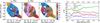 |
Fig. 7 Left panels: percentage contributions of young t< 140 Myr, intermediate (140 Myr <t< 1.4 Gyr) and old t> 1.4 Gyr stellar populations to the observed light at 5635 Å. Right panel: radial profiles of the light contributions from young xY (blue), intermediate xI (green) and old populations xO (red) with the radial distance in HLR and kpc. For comparison, the dashed lines with the same colors are the profiles for Sbc spiral galaxies from CALIFA. |
3.4. Results: Ages
The mean light-weighted log stellar age, ⟨ log age ⟩ L, was calculated using equation 3 in CF17.
Maps of ⟨ log age ⟩ L are shown in Fig. 6. From the CALIFA map we find that the youngest regions are the regions rich in star clusters located south of the nucleus, and the northern tidal tail, with mean ages around ~300 Myr. The nuclear region is ~500 Myr old, and the south tidal tail, and the eastern region of the main body, are older, with ages ~1 Gyr. In the circum-nuclear regions we find a positive trend of age with distance, from ~500 Myr in the nucleus itself to ~900 Myr at 1 HLR. It is also interesting to note that the full range of mean stellar ages is 140 Myr to less than 2 Gyr.
Again, when comparing the two datasets (LArr and PPaK), we find that they are indistinguishable from each other when considering the dispersion. At 0.5 ± 0.1 HLR, we find  (yr)= 8.75 ± 0.28 and
  (yr)= 8.85 ± 0.12.
The average light-weighted age of NGC 2623 at ~1 HLR is ~900 Myr, similar to the Sbc-Sc control galaxies. However, the nuclear region (within 0.2 HLR) of NGC 2623 is much younger, 500 Myr old, compared with the 3.6 Gyr (1.4 Gyr) age of the Sbc (Sc) control galaxies. Above 1 HLR, the mean stellar ages of NGC 2623 are similar to those in Sbc–Sc galaxies. The inner age gradient of NGC 2623 is positive with distance, in contrast with the negative gradient of Sbc–Sc galaxies: Δinage ~ 400 Myr, −2.4 Gyr, −670 Myr in NGC 2623, Sbc, and Sc galaxies, respectively. The early-stage mergers IC 1623 and NGC 6090 are, on average, younger than Sbc–Sc galaxies and NGC 2623. Moreover, their age profiles are significantly flatter than in Sbc–Sc galaxies, but not inverted as in NGC 2623.
If LIRGs were originally late-type spirals, then we conclude that the merger-induced star formation leads to a general rejuvenation of the progenitor galaxies during the early-stage merger stage that affects not only the central regions but also the “disk”. When the galaxies finally merge, most of the gas is already in the central regions and the young star formation is therefore concentrated there, whereas the outer parts are evolving passively. This would be consistent with the positive age gradient in NGC 2623.
3.5. Results: Contribution of young, intermediate, and old populations
In this section we study the spatially resolved SFH, by condensing the age distribution encoded in the population vector into three age ranges: young (YSP, t ≤ 140 Myr), intermediate age (ISP, 140 Myr <t ≤ 1.4 Gyr), and old stellar populations (OSP, t> 1.4 Gyr), as in CF17.
Figure 7 presents the maps (left) and radial profiles (right) of the light fractions at 5635 Å (the normalization λ) due to YSP, ISP, and OSP (xY, xI, and xO). In the right panels the blue, green, and red dashed lines are the contributions to light of YSP, ISP, and OSP of Sbc galaxies from the control sample.The contribution to light of the YSP is especially important in the center, the north tidal tail and in some places in the region rich in star clusters located south of the nucleus, with contributions to total light of ~40%. The ISP dominate the light almost everywhere (with contribution up to 70%). It is interesting to note the presence of the widespread ISP in this merger. The OSP are important to the southeast of the system, with contributions to light of ~40–50%. From the radial profiles we find that the light is dominated by ISP everywhere (0–3 HLR), with contributions of 50–70%, in contrast to the 20–40% in Sbc galaxies. We also find that within 0.5 HLR there exists a significant contribution to light by YSP, of ~20–30%, in contrast to the <10% YSP contribution in Sbc galaxies.
Similarly, in Fig. 8 we present the maps (left) and radial profiles (right) of the mass fractions due to YSP, ISP, and OSP (mY, mI and mO). The fraction of stellar mass contributed by YSP is less that 5% everywhere. Most of the mass is contained in OSP. In particular, OSP dominate the mass contributions within 1.5 HLR (50–80%), significantly smaller than the 84–96% contribution of OSP in Sbc galaxies. Beyond 1.5 HLR, the mass contribution of the ISP is also important, between 40 and 50%, and significantly higher than the 15% contribution of ISP to the mass in Sbc galaxies.
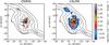 |
Fig. 9 OSIRIS Hα (left) and CALIFA Hα (right) emission line fluxes in units of 10-16 erg s-1 cm-2 arcsec-2 presented on a logarithmic scale. The black cone delimits the nuclear outflowing nebula reported by Lípari et al. (2004). The HST F555W image is shown in contours, smoothed to approximately match the spatial resolution of our IFS data. |
We have also computed the total mass in YSP, ISP, and OSP. Of the total stellar mass in NGC 2623 (5.4 × 10¹⁰M⊙), the mass in young, intermediate age, and old populations is 6.6 × 10⁸ (1%), 1.2 × 10¹⁰ (22%), and 4.1 × 10¹⁰M⊙ (77%), respectively.
The mass in young components (of ≲300 Myr) derived from the IFS data is comparable to the approximate mass in star clusters derived from the photometry, 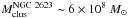 (see Appendix A). This supports the hypothesis that the vast majority of stars form in clusters rather than in isolation (Chandar et al. 2015).
4. Ionized gas emission
In this section we focus on the ionized gas properties. In order to account for stellar absorption, and to obtain pure nebular emission line spectra, we subtracted starlight best fits from the spectra. From the spectra we measured the line fluxes of the most prominent emission lines ([OII]λ3727, Hβ, [OIII]λ5007, [OI]λ6300, Hα, [NII]λ6584 and [SII]λλ6716,6731) by fitting them with Gaussian profiles. Emission-line intensity maps were thus created for each individual line. Only spaxels with signal to noise ratio (S/N) > 3 are considered in the following analysis. Hereafter, we focus only on the CALIFA IFS data, and on the higher-spatial-resolution Hα and [NII]λ6584 emission line maps from the OSIRIS TF (resolution ~1′′ compared with 2.4′′ for CALIFA).
4.1. Ionized gas morphology
Figure 9 shows the Hα maps derived from the OSIRIS (left panel) and CALIFA (right panel) data. These trace the distribution of ionized gas. The emission line distribution in the OSIRIS map is more compact than that in the CALIFA map, mainly due to its better spatial resolution. Moreover, we note that the CALIFA Hα emission has been corrected for the underlying stellar absorption, while this was not possible in OSIRIS data. We estimate that ~15% of the Hα flux is missing in OSIRIS data due to this. In NGC 2623 the vast majority of the ionized gas emission comes from the nuclear regions. Outside the nuclear regions, we detect three star forming clusters to the south, in the cluster-rich region found by Evans et al. (2008). The latter represents the youngest of the ~100 clusters in this region. Fainter Hα emission is also detected in the northern tidal tail, in both CALIFA and OSIRIS maps.
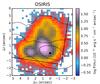 |
Fig. 10 Zoom of the OSIRIS Hα emission line image for the nuclear region of NGC 2623. HST continuum contours are overplotted in black. The black dot marks the continuum center. |
 |
Fig. 11 HST F555W continuum image of the nuclear region of NGC 2623 together with the OSIRIS Hα line emission plotted as red contours. The star cluster aggregations, A and B, and the HII regions, C1, C2, and C3 are labelled. The positions of the Hα lobe and SF associated to the tip of the lobe are also marked. |
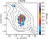 |
Fig. 12
|
Lípari et al. (2004, hereafter L04) reported convincing evidence of the existence of an outflow due to a nuclear dusty starburst in this system, leaning on the broad (FWHM ~ 600 km s-1), blueshifted (~–400 km s-1) and highly asymmetric line profiles at extranuclear locations (see their Figs. 7, and 11 bottom). The enhanced [NII]/Hα ratio, is also consistent with a scenario in which a different excitation mechanism, most naturally shocks, dominates at the location of the outflowing gas. The orientation and location of the outflow, as reported by L04, are indicated with black solid lines in Fig. 9. A cone-shaped nebula is formed, with an opening angle of θ ~ 100°.
With respect to the morphology, and given the higher spatial resolution of the OSIRIS map, we are able to distinguish substructures within the cone-nebula that are unresolved in the CALIFA and L04 maps. Figure 10 zooms in on the nuclear regions of the OSIRIS Hα map. Also, to get a better idea of the overall morphology of the cone nebula, in Fig. 11 we have superimposed in red contours the OSIRIS Hα emission over the HST F555W continuum image. Within the cone nebula, we notice different structures. There is a point-like source offset with respect to the continuum center by (2.7′′E, 0.1′′N, label A in Fig. 11). Its morphology is consistent with a star forming knot, also confirmed by the line-ratios ([NII]/Hα ~ 0.5, and [OIII]/Hβ ~ 1.25). There is also an extended lobe-like emission region with bow-shaped, clumpy ends that seems to emerge from the nucleus. This kind of morphology is typical of shocked regions. Inside this lobe, we find that the brightest Hα emission corresponds to several cluster aggregations, labeled B in Fig. 11. Most of the extended Hα emission is spatially coincident with highly obscured regions. Some bright clusters appear at the tip of the lobe (at the “edges” of the outflow), whose formation might have been induced by the outflow. Finally, the three HII regions south of the nucleus (C1, C2, and C3) are also indicated in the figure, and their stellar counterparts are clearly detected.
4.2. [SII]-based gas densities
We have estimated the electron density of the emitting gas (ne) in the center of NGC 2623, using the ratio [SII]λ6716/[SII]λ6731, and applying Osterbrock & Ferland (2006) calibration assuming an electron temperature of T = 104 K. On average, the ratio is around the low density limit (~1.4 ± 0.1), indicating densities of ~100 cm-3 or lower. The ratio has a value of around 1.25 ± 0.08 in the nucleus itself, equivalent to an electron density of 189 ± 97 cm-3.
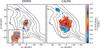 |
Fig. 13 Left: emission line ratio map of [NII]λ6584/Hα derived from the OSIRIS data. The box in the lower left corner is a zoom of the nuclear region. Right: [NII]λ6584/Hα derived from the CALIFA data. |
4.3. Ionized gas dust attenuation
We estimate the nebular extinction,  , assuming an intrinsic ratio of I(Hα)/I(Hβ) = 2.86, valid for Case B recombination for an electron temperature T = 10 000 K and an electron density 102 cm-3 (Osterbrock & Ferland 2006), typical of star forming regions. We used the Calzetti et al. (2000) reddening function, which works better for starburst galaxies.
In Fig. 13 we show the map. The highest extinction is found in the nuclear regions, where is up to 4.5 mag. This level of extinction implies that a dust screen with high covering fraction lies in front of the central region of the galaxy, consistent with the dust lanes visible in the HST images. However, the ionized gas in the northern tidal tail and in the clusters south of the nucleus has  mag. The global average is
  mag.
mag.
We have compared the ratio of the nebular and the stellar extinction using the spaxels where the S/N of Hα and Hβ is above 3, and  mag, and find an average of
  . This result is in agreement with what we found in the early-stage merger LIRGs IC 1623 W and NGC 6090, and with other results from the literature (Calzetti et al. 1994; Kreckel et al. 2013).
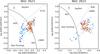 |
Fig. 14 [NII]λ6584/Hα vs. [OIII]λ5007/Hβ (left panel), and [OI]λ6300/Hα vs. [OIII]λ5007/Hβ (right panel) line ratio diagnostic diagrams. Spaxels are color-coded according to the Hα velocity dispersion map shown in Fig. 15. Solid lines in both diagnostic diagrams mark the “maximum starburst lines” obtained by Kewley et al. (2001, K01) by means of photoionization models of synthetic starbursts; the dotted line in the left panels marks the pure SDSS star-forming galaxies frontier semi-empirically drawn by Kauffmann et al. (2003, K03); and the dashed-dotted lines that separate Seyferts from LINERs are from Cid Fernandes et al. (2010, CF10) and Kewley et al. (2006, K06). The average error bars are shown in the top-left corners. |
4.4. Emission line ratios sensitive to ionization source
Standard line ratios sensitive to the shape of the ionizing spectrum have been calculated.
First, we note that the [OIII]λ5007/Hβ ratio is below ~2 everywhere. Higher values would be expected for Seyfert-like emission (Heckman et al. 1987; Veilleux et al. 1995). We point out that in our spatially resolved observations, the emission lines do not show Seyfert-like line ratios, not even in the nuclear region (see also following section). Although X-ray and IR data point to the existence of an AGN embedded in dust within the inner kiloparsec of the system, the bulk of infrared (and thus bolometric) luminosity is generated by star formation (Evans et al. 2008; Petric et al. 2011).
In Fig. 13 we show the [NII]λ6584/Hα maps for OSIRIS data (left) and CALIFA data (right). The lowest values of the ratio are found in the north tidal tail and in the three star forming knots south of the nucleus (C1, C2, and C3). The CALIFA ratios are consistent with those derived from the OSIRIS data, but less sensitive to small-scale variations due to the coarser spatial resolution. With the greater spatial resolution of OSIRIS, we see finer details of the ionization in the nuclear region of NGC 2623. In particular, inside the L04 cone nebula, the nuclear knot (A), and some pixels at the clumpy ends of the nuclear lobe, are also consistent with star formation ionization ([NII]/Hα ~ 0.5), while the remainder have [NII]/Hα between 1.0 and 1.2. For the spaxels at the edges of the cone nebula, the [NII]/Hα ratio is even larger, with values in the range 1–2, which could be associated with the effects of shocks produced by the outflow colliding with the ISM (Heckman et al. 1987, 1990).
We note that our measurements are in perfect agreement with those reported by L04 inside the cone nebula. However, outside the cone nebula, L04 report values of [NII]/Hα> 3, which is not consistent with our results. As previously mentioned, in L04 the Hα flux is not corrected for the underlying stellar absorption, and therefore the Hα flux is underestimated, leading to higher values of this ratio. This effect is stronger outside the cone nebula, where the Hα emission is weaker. From the IFS we calculate that 20–25% of the Hα flux is underestimated when not correcting from the stellar absorption, and the morphology is more compact and more similar to L04 and the OSIRIS map in that case. We note that the IFS is highly appropriate for this kind of analysis.
The [OI]λ6300/Hα and [SII]λλ6716+6731/Hα maps inside the cone nebula have values ~0.2 and ~0.5, respectively, consistent with L04. Following Heckman et al. (1990), these values are indicative of shock-heated gas of moderate velocity. These results are confirmed by the diagnostic diagrams shown in the following Section.
4.5. Diagnostic diagrams
We have used diagnostic diagrams to identify the nature of the dominant ionization mechanisms. Figure 14 presents two diagrams: [NII]λ6584/Hα versus [OIII]λ5007/Hβ (left panel, the “BPT diagram”, Baldwin et al. 1981), and [OI]λ6300/Hα versus [OIII]λ5007/Hβ (right panel, Veilleux & Osterbrock 1987). The spaxels are colored according to their Hα velocity dispersion (σHα), following the scale shown in the σHα map in Fig. 15 (top panel).
Overplotted as black lines are empirically and theoretically derived separations between LINERs/Seyferts and HII regions. The dotted line is from Kauffmann et al. (2003), a conservative demarcation to separate SDSS star forming galaxies from those hosting an AGN; the solid line is from Kewley et al. (2001), marking the “maximum starburst lines” derived using the results of photoionization models of synthetic starbursts. Finally, the dashed-dotted lines that separate Seyferts from LINERs are from Cid Fernandes et al. (2010) and Kewley et al. (2006).
Only the northern tidal tail and the brightest knot south of the nucleus have line ratios consistent with pure stellar photoionization. On the other hand, the gas inside the nuclear cone defined by L04 has LINER-like emission lines. This is consistent with the presence of the outflow reported by L04. In general, the higher the velocity dispersion, the more LINER-like the ionization is, suggesting shocks as the cause, as previously found in other local U/LIRGs (Monreal-Ibero et al. 2006; Rich et al. 2014), and in the two LIRGs in CF17. An ensemble of HII regions would not be able to reproduce the line ratios we observe. However, many spaxels fall in the composite region of the BPT, and according to the highest resolution OSIRIS and HST data, a collection of HII regions is also present in the plane of the galaxy. Thus, the presence of both an outflow and HII regions is necessary to explain the morphology and mixture of ionization mechanisms. In addition, we note that there is also a region to the west of the nucleus with line ratios consistent with LINER-like ionization, although this region has a low velocity dispersion, more typical of HII regions.
4.6. Gas kinematics
We have determined the kinematics of the ionized gas in NGC 2623 using the Gaussian fits to Hα. To obtain the final velocity dispersion, we subtracted the CALIFA instrumental resolution (σinst) in quadrature, where σinst at Hα is ~116 km s-1. Therefore, line widths below ~58 km s-1 are unresolved at the CALIFA resolution.
The Hα velocity dispersion map is shown in the top panel of Fig. 15. σHα is low (<100 km s-1) in the star forming regions to the south of the nucleus, and in the northern tidal tail. The highest values of the velocity dispersion are reached inside the cone nebula defined by L04 (up to 220 km s-1). This high sigma could be a simple consequence of the two velocity components in Hα found by L04, that clearly prove the presence of an outflowing gas in NGC 2623. In our data, which have worse spectral resolution, these two components are convolved into a unique Hα line, that is significantly broader than in the surrounding ionized gas4. Obviously, a fraction of the broadening may also be due to unresolved non-circular motions in the disk and/or to unresolved central rotation due to beam smearing. However, since the data of L04 prove so clearly the existence of an outflow, we are tempted to interpret our sigma map as a consequence of this outflow.
In the bottom panel of Fig. 15 we show the Hα velocity field. A rotation pattern is preserved in the nucleus, with an amplitude of ±120 km s-1, in agreement with Barrera-Ballesteros et al. (2015). We have found that the kinematic center is displaced 2 arcsec to the east with respect to the photometric center. However, this is within our spatial resolution. The position angles of the kinematic major axis for the approaching and receding sides calculated by Barrera-Ballesteros et al. (2015) are shown in the figure with black solid lines. For NGC 2623, PA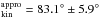 and PA
 . Beyond the nucleus, both the star forming regions in the north tidal tail and the material in the cluster-rich region to the south are approaching us at ~40 km s-1.
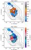 |
Fig. 15 Top panel: velocity dispersion derived from Hα, corrected for the instrumental width (σinst ~ 116 km s-1). Bottom panel: velocity field derived from Hα. The position angles of the kinematic major axis for the approaching and receding sides have been calculated by Barrera-Ballesteros et al. (2015) and are shown in the figure with black solid lines. The circle in the top right corner of both maps represents the spatial resolution, given by the diameter of PPaK fibres, ~2.7′′. |
4.7. OSIRIS line emission at the edge of the SW tidal tail
The OSIRIS narrow-band filter imaging data covers a very large FoV, including the full extent of NGC 2623, beyond the tidal tails. In the OSIRIS 6720 Å and 6725 Å filter maps (6580 and 6585 Å rest-frame at NGC 2623 center), we detect four regions located more than 19 kpc away from the center, at the edge of the southwestern tidal tail.
As mentioned in Sect. 2.2, the wavelength tuning is not uniform over the full field of view of OSIRIS. There is a progressively increasing shift to the blue of the central wavelength (λ0) as the distance (r) from the optical center increases. At the positions of the four extended regions in the OSIRIS FoV, the filter is sensitive to emission at wavelengths ranging from 6553 to 6562 Å, corresponding to rest-frame [NII]λ6548 and Hα emission; the measured fluxes in these regions are in the range 2.5–7.7 × 10⁻¹⁶ erg s-1 cm-2. The line emission indicates that these are (presumably young) star forming regions.
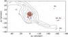 |
Fig. 16 OSIRIS ~6723 Å map emission flux image derived from the OSIRIS data. This corresponds to the [NII]λ6584 rest frame at the NGC 2623 center, and to between [NII]λ6548 and Hα emission in R1, R2, R3, and R4. |
In Fig. 16 we show the average of the OSIRIS 6720 Å and 6725 Å maps, where the star forming regions have been indicated as R1, R2, R3, and R4. The latter were previously detected in Hα and UV images of NGC 2623 by Bournaud et al. (2004) and de Mello et al. (2012), respectively. We note that these regions do not coincide with the optical emission from the southern tidal tail. Instead, they are embedded in the underlying southern HI tail, which is located far away from the stellar component of NGC 2623, as found by Hibbard & Yun (1996). According to the HI kinematics, the southern HI tail is bending towards the North, incorporating the four star-forming regions. The two brightest (R2 and R3) are near to the HI emission peak, as can be seen in de Mello et al. (2012). A similar case is given by the late-stage merger NGC 7252 (Lelli et al. 2015), where there are two genuine tidal dwarf galaxies (TDGs) in formation. Through a detailed analysis of the gas dynamics and metallicity in this system, using HI and optical IFS observations, they reinforce that the TDGs in NGC 7252 were not pre-existing dwarfs, but currently forming out of pre-enriched material ejected from the progenitor galaxies. Moreover, they found evidence of TDGs being devoid of dark matter.
Given the location of R1–R4 star forming regions in NGC 2623, they are compatible with the formation of a tidal dwarf galaxy in the south-west tail of NGC 2623. Unfortunately, we cannot characterize them further, because these regions are not covered by the CALIFA data cube, and so we cannot estimate their kinematics, and precise masses, ages, and metallicities.
5. Discussion
Interactions, and, in particular, mergers, enhance star formation, leading to star formation rates (SFRs) that are temporarily increased, sometimes by large amounts. Evolved mergers like NGC 2623, are ideal systems for characterizing and quantifying merger-induced star formation in order to further elucidate the evolutionary path followed by major mergers. In this section we discuss our main findings in the context of the merger-driven evolution of galaxies.
5.1. Global enhancement of the star formation
First, we calculate and compare the current SFR of NGC 2623, using the spectral synthesis, Spitzer 24 μm, FIR and radio continuum data.
The current SFR in different timescales (tSF = 30 Myr, 1 Gyr) is obtained using the SFH derived from the stellar continuum decomposition, by adding all the stellar mass formed in the last tSF, and dividing it by this time. We also used public IR data (MIPS 24 μm from Spitzer, and IRAS 25, 60, and 100 μm) and radio continuum (Very Large Array, VLA at 1.4 GHz) to derive the current average SFR. Using Kennicutt et al. (2009) hybrid calibrations, we found that the three of them lead to an average SFR ~ 18 M⊙ yr-1, with a small dispersion of 1 M⊙ yr-1. This value is similar to SFR estimated from the spectral synthesis for tSF = 1 Gyr (SFR ~ 12 M⊙ yr-1), and a factor 2 above if the SFR is calculated in the very recent past (tSF = 30 Myr) (SFR ~ 8 M⊙ yr-1). The difference in the SFR calculated with different indicators is a consequence of the SFR not being constant in the recent past of this galaxy, as the star formation history shows. However, the observed discrepancies are within the dispersion of ~0.2 dex found by Pereira-Santaella et al. (2015) when they compare the SFR derived from the FIR emission with SFR from the star formation history over the timescale of ~100 Myr in a sample of LIRGs.
These calculations show that the SFR in NGC 2623 is enhanced by a factor 2–3 with respect to main sequence star forming galaxies (González Delgado et al. 2016), and similar to the global enhancement of the star formation found in the pre-merger LIRGs IC 1623 and NGC 6090 (CF17).
5.2. Merger-induced star formation and evolutionary scheme
Another important aspect of mergers that must be taken into account is the spatial extension of the star formation. We have used multi-wavelength imaging from FUV to NIR to characterize the star cluster properties in NGC 2623 (see Appendix A). Our analysis shows that NGC 2623 has experienced at least two recent major episodes of massive cluster formation: one in the innermost nuclear regions (within 0.5 HLR ~ 1.4 kpc) in the last ≲100 Myr, and other ~250 Myr ago in the off-nuclear regions and some clusters in the circum-nuclear region (Sect. A.1). When considering only the optical colours, our results are in agreement with Evans et al. (2008). However, we find that the age estimates can be improved by including the UV data.
Moreover, the cluster ages derived by us are consistent with the first dynamical simulation for NGC 2623 developed by Privon et al. (2013), predicting that the first peri-center passage occurred 220 Myr ago, while the coalescence occurred 80 Myr ago. Similar results are found in other evolved mergers, such as Arp 220 and NGC 7252 (Miller et al. 1997; Wilson et al. 2006), while in contrast, in early-stage mergers such as the Antennae, IC 1623 and NGC 6090, the young stellar populations are not so centrally concentrated, but widespread over several kpc scales (Zhang et al. 2001; Cortijo-Ferrero et al. 2017).
From our IFS, we have also found that young stellar populations (<140 Myr) are mainly located in the innermost (<0.5 HLR ~ 1.4 kpc) central regions; while a previous and widespread (~2 HLR ~ 5.6 kpc) episode is traced by the spatially extended intermediate-age stellar populations with ages between 140–1.4 Gyr (Fig. 7). Due to this distribution of the stellar populations, the center of NGC 2623 (<0.2 HLR) is younger (500 Myr on average) than at 1 HLR (~900 Myr) (Fig. 6), and the age gradient in the inner 1 HLR, Δinage, is positive (~400 Myr), in contrast with the negative gradients in Sbc–Sc galaxies (−2.4 Gyr/−670 Myr). The stellar extinction is high in the inner 0.2 HLR (~1.4 mag), and shows a negative gradient, which is much steeper (–0.9 mag) than in Sbc-Sc galaxies, −0.3 mag (Fig. 5).
Other studies based on long-slit spectroscopy have found a similar distribution of the stellar populations in ULIRGs, including also the prototypical Arp 220 (Rodríguez Zaurín et al. 2008, 2009).
The enhancement of the star formation and the spatial distribution of the stellar populations in NGC 2623 supports the evolutionary scheme proposed in CF17 for two early-stage mergers. In this scheme, some star formation is initially triggered in the central regions during the first contact stage, followed by extended star formation after the first peri-center passage. In NGC 2623, we are observing the fossil record of this extended population (which is already a few 100 Myr to 1 Gyr old), a relic of when NGC 2623 was at an earlier merger stage. This result is also in agreement with high-resolution models in the literature (Teyssier et al. 2010; Hopkins et al. 2013; Renaud et al. 2015), which apart from the extended star formation, also predict a later nuclear starburst between the second peri-center passage and the final coalescence, which is exactly what we find in NGC 2623.
We emphasize that understanding the onset and evolution of star formation in mergers requires further observational studies. Not all early-stage mergers present extended and significant young star formation, as is the case of the post first passage Mice galaxies (Wild et al. 2014). In a future paper we aim to extend the sample to cover more early-stage mergers and merger systems, in order to observationally trace the star formation in mergers and put further constraints on the simulations.
5.3. Ionized gas distribution and ionization mechanism
Most of the ionized gas in NGC 2623 is concentrated in the nuclear regions (≲1 HLR), in contrast with the two early-stage merger LIRGs studied in CF17, where the young stellar components are more widespread. This reinforces the idea that the young stellar components are mostly located in the central regions for advanced, post-coalescence systems.
This result found for NGC 2623 is supported by Hattori et al. (2004), who found that, in separated pairs, the contribution of extended starbursts (>1 kpc) to the Hα emission is important, while in mergers (single coalesced nucleus), the nuclear starbursts are very compact (from 100 pc–1 kpc) with no, or negligible, star forming activity in the outer regions. Analogously, García-Marín et al. (2009), Arribas et al. (2012) found that in the pre-coalescence systems, the size of the Hα-emitting region is above 2 kpc and up to 7–8 kpc, while for the post-coalescence systems it is <2 kpc.
From the diagnostic diagrams we find that only the line ratios of gas in the northern tidal tail and in the brightest knot south of the nucleus are consistent with pure stellar photoionization. In the outflow cone nebula we find LINER-like ionization, together with the highest values of the velocity dispersion (~220 km s-1). An ensemble of HII regions alone would not be able to reproduce the line ratios we observe, and shock contribution from the outflow is necessary. However, we find that a collection of star forming regions is also present, and coexists with the outflow in the plane of the galaxy. Extended shock excitation has been previously found in many local U/LIRGs. Closely interacting pairs and coalesced mergers show a high velocity dispersion component, above 100 km s-1, and an increasingly dominant contribution from composite and LINER-like emission line ratios, tracing an increasing fractional contribution from shocks, exceeding half of the Hα luminosity in late-stage coalesced mergers (Rich et al. 2015).
5.4. Intensity of the SFR and outflow escape
Using the Hα luminosity of the shocked regions (i.e., spaxels with LINER-like ionization,  erg s-1) we made an independent estimation of the current SFR which would be necessary to power the outflow. We have converted L
 into a bolometric energy loss rate Ėshock ~ 2.0 × 1043 erg s-1 5, in order to compare with the mechanical energy released to the ISM by SNe from evolutionary synthesis models (Leitherer et al. 1999). Assuming a continuous SFR, with a Salpeter IMF, and an average metallicity of ~0.7 Z⊙ (estimated from the spectral synthesis), we find that a SFR of ≲26 M⊙ yr-1 is required to power the observed outflow. This value is consistent with the SFR predicted from multi-wavelength data (~18 M⊙ yr-1), and represents an upper limit because some star formation contribution to the Hα emission is also expected.
It is also interesting to know if NGC 2623 outflow is able to escape the galaxy and contribute to the ionization/enrichment of the intergalactic medium. In principle, it seems unlikely given the low SFR intensity of ~0.5 M⊙ yr-1 kpc-2 of NGC 2623. However, Arribas et al. (2014) found that, while high-z galaxies seem to require ΣSFR> 1 M⊙ yr-1 kpc-2 to launch strong outflows, this threshold is not observed in low-z U/LIRGs.
Following Colina et al. (1991), we estimate the total amount of ionized outflowing gas from the  above, and the electron density estimated in the cone-nebula Ne ~ 100 cm-3, which leads to Mg ~ 1.1 × 10⁷M⊙ (Chabrier IMF). L04 derived an outflow velocity of ⟨ VOF ⟩ ~ −405 km s-1, that, together with the radius of the outflowing region in kpc (r = 1.4 kpc), allows us to calculate the dynamical time, tdyn ~ 3.4 × 10⁶ yr, and the outflow rate,
  /yr (Chabrier IMF), which is a factor 3 lower than the SFR (~11 M⊙/yr, Chabrier IMF). We also find that the outflow velocity is smaller than the escape velocity in the central areas, with an average Vesc ~ 570 ± 70 km s-1 6>⟨ VOF ⟩. These results indicate that in this case the outflow cannot escape and will be retained within the galaxy.
5.5. NGC 2623 and the formation of an elliptical galaxy
Several studies have proposed that major mergers end up forming elliptical (E) galaxies. Kormendy & Sanders (1992) were the first to propose that U/LIRGs evolve into E through merger-induced dissipative collapse. U/LIRGs have large molecular gas concentrations in their central kpc regions (Downes & Solomon 1998) with densities comparable to stellar densities in E. They lie on the fundamental plane in the same region as intermediate mass E (Genzel et al. 2001), and their NIR brightness profiles follow a de Vaucouleurs r1 / 4 law (Wright et al. 1990; Scoville et al. 2000).
There is also evidence in the literature that NGC 2623 could evolve into an elliptical galaxy. This evidence comes from a) the average rotation curve, which is well fitted by a Plummer spherical potential (L04) and b) the NIR light surface brightness profile of the central region, which is well fitted by the r1 / 4 law by Scoville et al. (2000) using NICMOS data. However, this last study also indicates that an exponential law can also fit well the NIR light distribution if the central region (<2 kpc) is excluded.
Our analysis provides additional information about the future evolution of this LIRG/merger system. In Sect. 3.2 we found that the radial distribution of the stellar mass surface density is quite similar to Sbc galaxies in CALIFA, which are significantly less dense than massive E galaxies. Furthermore we found that its central gradient (Δinlog μ⋆ = −1.2) is flatter than the gradient in massive (M⋆> 1011M⊙) E–S0 galaxies (Δin log μ⋆ = −1.4, GD15). Because this difference in the gradient with respect to E–S0 galaxies could be due to an insufficient extinction correction or to the limited spatial resolution in the inner regions, we proceeded as follows. Using the SFH history derived from the spectral fits, we estimated the synthetic radial profile of the 1.6 μm luminosity surface density, and compared it with the NICMOS F160W luminosity surface brightness. We find that both radial profiles are very similar, and there only exists a discrepancy in the innermost 0.25 HLR, where the NIC2/NIC3 F160W profile is slightly steeper. This discrepancy is easily explained by the worse spatial resolution of our IFS data in comparison with NICMOS. This prevents us from tracing the inner steep rise of the radial profile with the IFS, while outside of >0.7 HLR we find an exponential profile, in agreement with Scoville et al. (2000) (Appendix C and Fig. C.1).
As an additional check, we explicitly extracted the mass surface-density profiles of E/S0, Sa, and Sb galaxies in the CALIFA sample with stellar masses in the same mass range as NGC 2623 (3 × 10¹⁰–8 × 10¹⁰M⊙). The E/S0 sub-sample of intermediate mass is now more similar to NGC 2623, with a global difference in the mass surface density of ~0.3 dex, and ∇inlog μ⋆ = −1.3, which is closer to the ∇in log μ⋆ in NGC 2623. Thus, our conclusion is that if NGC 2623 forms an E, it has to be less massive than 1011M⊙. Alternatively, we cannot discard the possibility that NGC 2623 will end up as a spiral galaxy with a prominent bulge, because ∇in log μ⋆ is also similar to Sa–Sb galaxies (Fig. 17). Recent simulations have found that gas-rich major mergers can also produce spiral remnants. The stellar progenitor disks are first destroyed by violent relaxation during the mergers, forming classical bulges, but new disks soon regrow out of the leftover debris, as well as gas accreted mainly from the haloes (Springel & Hernquist 2005; Athanassoula et al. 2016).
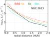 |
Fig. 17 Radial profile of log μ⋆ for NGC 2623 (black line) and for a sub-sample of E/S0 and spiral galaxies from the CALIFA survey that have a stellar mass (10.5 ≤ log M⋆ (M⊙) ≤ 10.9) similar to NGC 2623. |
6. Summary and conclusions
We have characterized the star cluster properties, the stellar population, the ionized gas properties, and the ionization mechanism of the merger LIRG NGC 2623 by analyzing high quality IFS data from PMAS LArr and CALIFA, in the rest-frame optical range 3700–7000 Å, high-resolution HST imaging, as well as OSIRIS narrow band Hα and [NII]λ6584 imaging. NGC 2623 results have been compared to control Sbc and Sc galaxies from CALIFA (GD15) in the same mass range, and to the early-stage merger LIRGs IC 1623 W and NGC 6090 studied in CF17. Our main results are as follows.
-
–
From the IFS and clusters photometry we find two periods ofmerger-induced star formation in NGC 2623: Arecent episode, traced by YSPs (<140 Myr), and located in the innermost (<0.5 HLR ~ 1.4 kpc) central regions and in some isolated clusters in the northern tidal tail and to the south of the nucleus; and an earlier and more widespread (~2 HLR ~ 5.6 kpc) episode, traced by the spatially extended ISPs (between 140 Myr and 1.4 Gyr). This result is consistent with the epochs of the first peri-center passage (~200 Myr ago) and coalescence (<100 Myr ago) predicted by dynamical models, and in agreement with high-resolution merger simulations in the literature.
-
The central region (inner 0.2 HLR) shows the highest extinction with
 mag. Moreover, in the inner 1 HLR, there exists a negative
  gradient which is much steeper in NGC 2623 (−0.9 mag) than in Sbc/Sc galaxies (−0.3 mag). This is in contrast to the flat profiles in the early-stage merger LIRGs, and is consistent with the idea that, in mergers with coalesced nuclei, most of the dust content is already concentrated in the central regions.
 -
The age gradient of NGC 2623 in the inner 1 HLR, Δinage, is positive (~400 Myr), in contrast to the negative gradient found in Sbc/Sc galaxies (−2.4 Gyr/−670 Myr). The positive age gradient could be explained in advanced mergers if most of the gas/star formation is concentrated in the center, while the outer parts evolve passively.
-
Only gas in the northern tidal tail and the brightest knot south of the nucleus are purely ionized by young massive stars. In the nuclear region of NGC 2623, we find LINER-like ionization and high values of the velocity dispersion (~220 km s-1), consistent with shock excitation associated with a known outflow. As revealed by the highest-resolution OSIRIS and HST data, a collection of HII regions is also present in the plane of the galaxy, which explains the mixture of ionization mechanisms in this system.
-
The three hybrid tracers (observed Hα from the IFS, together with 24 μm, FIR, and radio 1.4 GHz), lead to an average SFR ~ 18 M⊙ yr-1 (Salpeter IMF), similar to the one derived from the spectral synthesis, averaging in the last 1 Gyr, SFR (<1 Gyr) ~12 M⊙ yr-1.
-
The low SFR intensity (~0.5 M⊙ yr-1 kpc-2), the fact that the outflow rate is three times lower than the current SFR, and the escape velocity in the central areas higher than the outflow velocity, all suggest that NGC 2623 outflow cannot escape and will be retained within the galaxy.
-
The stellar mass density profile of NGC 2623 resembles that of Sbc galaxies in the CALIFA sample, and is, globally, 0.6 dex less dense than E–S0. These results indicate that NGC 2623 may form a low-intermediate-mass E (log M⋆ ≲ 11) but not a very massive one, or, consistently with recent simulations, a spiral galaxy with a prominent bulge (Sa–Sbc).
The ratio of the stellar masses derived with GM and CB models, M⋆(GM) /M⋆(CB) = 2.25, is larger than the 1.78 value expected due to the different IMFs (Salpeter vs. Chabrier). This is because this ratio is also affected by the differences in the stellar population properties, especially the stellar ages. This is shown in Appendix B, where we discuss the uncertainties related to the models choice.
The HLR is defined as the length of the radial aperture which contains half of the total light of the galaxy at the rest-frame wavelength.
We have analyzed in more detail the Hα+[NII] line profiles in the outflow region and found that they are better fit when including a second broad (FWHM ~ 670 km s-1) component, blueshifted by ~–200 km s-1 with respect to the narrow systemic component. The two components fit leaves less residuals than the one component fit, in agreement with L04 findings.
Assuming that the bolometric conversion factor for the shocks in NGC 2623 (~400 km s-1) can be approximated by that computed by Rich et al. (2010) for low-velocity shock models, which tends to ~80 for vshock = 140–200 km s-1.
Using Eq. (7) of Arribas et al. (2014), assuming rmax = 10 kpc, and following Eq. (1) of Bellocchi et al. (2013) to derive the dynamical mass of NGC 2623 inside the inner 1 half mass radius (2.2 kpc, σmean ~ 131 km s-1), which is ~5.3 × 10¹⁰M⊙, with a factor 1.3 of uncertainty, similar to the dynamical mass estimated by Privon et al. (2013).
Although we focus on the GM base results throughout the paper, GM SSPs spectra only cover the optical range while CB SSPs spectra extent all the way to the NIR 1.6 μm, and so we use CB in this comparison.
Acknowledgments
CALIFA is the first legacy survey carried out at Calar Alto. The CALIFA collaboration would like to thank the IAA-CSIC and MPIA-MPG as major partners of the observatory, and CAHA itself, for the unique access to telescope time and support in manpower and infrastructures. We also thank the CAHA staff for the dedication to this project. Support from the Spanish Ministerio de Economía y Competitividad, through projects AYA2016-77846-P, AYA2014-57490-P, AYA2010-15081, and Junta de Andalucía FQ1580. ALdA, EADL, and RCF thank the hospitality of the IAA and the support of CAPES and CNPq. R.G.D. acknowledges the support of CNPq (Brazil) through Programa Ciência sem Fronteiras (401452/2012-3). M.V.M. acknowledges support from Spanish MINECO through grant AYA2015-64346-C2-2-P. C.C.F. acknowledges the constructive comments from Carlos López-Cobá and Salvador Duarte Puertas. This research made use of Python (http://www.python.org); Numpy (Van Der Walt et al. 2011), and Matplotlib (Hunter 2007). We thank the anonymous reviewer for his/her careful reading of our manuscript and the insightful comments and suggestions.
References
- Alvensleben, U. F. 2004, The Formation and Evolution of Massive Young Star Clusters, ASP Conf. Ser., 322, 91 [NASA ADS] [Google Scholar]
- Athanassoula, E., Rodionov, S. A., Peschken, N., & Lambert, J. C. 2016, ApJ, 821, 90 [NASA ADS] [CrossRef] [Google Scholar]
- Armus, L., Heckman, T. M., & Miley, G. K. 1989, ApJ, 347, 727 [NASA ADS] [CrossRef] [Google Scholar]
- Arribas, S., Colina, L., Alonso-Herrero, A., et al. 2012, A&A, 541, A20 [NASA ADS] [CrossRef] [EDP Sciences] [Google Scholar]
- Arribas, S., Colina, L., Bellocchi, E., Maiolino, R., & Villar-Martín, M. 2014, A&A, 568, A14 [NASA ADS] [CrossRef] [EDP Sciences] [Google Scholar]
- Baldwin, J. A., Phillips, M. M., & Terlevich, R. 1981, PASP, 93, 5 [NASA ADS] [CrossRef] [EDP Sciences] [Google Scholar]
- Barrera-Ballesteros, J. K., García-Lorenzo, B., Falcón-Barroso, J., et al. 2015, A&A, 582, A21 [NASA ADS] [CrossRef] [EDP Sciences] [Google Scholar]
- Bastian, N., Saglia, R. P., Goudfrooij, P., et al. 2006, A&A, 448, 881 [NASA ADS] [CrossRef] [EDP Sciences] [Google Scholar]
- Bell, E. F., McIntosh, D. H., Katz, N., & Weinberg, M. D. 2003, ApJS, 149, 289 [NASA ADS] [CrossRef] [Google Scholar]
- Bellocchi, E., Arribas, S., Colina, L., & Miralles-Caballero, D. 2013, A&A, 557, A59 [NASA ADS] [CrossRef] [EDP Sciences] [Google Scholar]
- Bernloehr, K. 1993, A&A, 268, 25 [NASA ADS] [Google Scholar]
- Bournaud, F., Duc, P.-A., Amram, P., Combes, F., & Gach, J.-L. 2004, A&A, 425, 813 [NASA ADS] [CrossRef] [EDP Sciences] [Google Scholar]
- Bruzual, G., & Charlot, S. 2003, MNRAS, 344, 1000 [NASA ADS] [CrossRef] [Google Scholar]
- Calzetti, D., Kinney, A. L., & Storchi-Bergmann, T. 1994, ApJ, 429, 582 [NASA ADS] [CrossRef] [Google Scholar]
- Calzetti, D., Armus, L., Bohlin, R. C., et al. 2000, ApJ, 533, 682 [NASA ADS] [CrossRef] [Google Scholar]
- Cappellari, M., & Copin, Y. 2003, MNRAS, 342, 345 [NASA ADS] [CrossRef] [Google Scholar]
- Chandar, R., Fall, S. M., & Whitmore, B. C. 2015, ApJ, 810, 1 [NASA ADS] [CrossRef] [Google Scholar]
- Cid Fernandes, R., Stasińska, G., Schlickmann, M. S., et al. 2010, MNRAS, 403, 1036 [NASA ADS] [CrossRef] [Google Scholar]
- Cid Fernandes, R., Pérez, E., García Benito, R., et al. 2013, A&A, 557, A86 [NASA ADS] [CrossRef] [EDP Sciences] [Google Scholar]
- Cid Fernandes, R., González Delgado, R. M., García Benito, R., et al. 2014, A&A, 561, A130 [NASA ADS] [CrossRef] [EDP Sciences] [Google Scholar]
- Colina, L., Lipari, S., & Macchetto, F. 1991, ApJ, 379, 113 [NASA ADS] [CrossRef] [Google Scholar]
- Cortijo-Ferrero, C., González Delgado, R. M., Pérez, E., et al. 2017, MNRAS, 467, 3898 [NASA ADS] [CrossRef] [Google Scholar]
- Davies, R. L., Medling, A. M., U, V., et al. 2016, MNRAS, 458, 158 [NASA ADS] [CrossRef] [Google Scholar]
- de Mello, D. F., Urrutia-Viscarra, F., Mendes de Oliveira, C., et al. 2012, MNRAS, 426, 2441 [NASA ADS] [CrossRef] [Google Scholar]
- Di Matteo, P., Combes, F., Melchior, A.-L., & Semelin, B. 2007, A&A, 468, 61 [NASA ADS] [CrossRef] [EDP Sciences] [Google Scholar]
- Di Matteo, P., Bournaud, F., Martig, M., et al. 2008, A&A, 492, 31 [NASA ADS] [CrossRef] [EDP Sciences] [Google Scholar]
- Downes, D., & Solomon, P. M. 1998, ApJ, 507, 615 [NASA ADS] [CrossRef] [Google Scholar]
- Elmegreen, D. M., Elmegreen, B. G., Kaufman, M., et al. 2006, ApJ, 642, 158 [NASA ADS] [CrossRef] [Google Scholar]
- Evans, A. S., Vavilkin, T., Pizagno, J., et al. 2008, ApJ, 675, L69 [NASA ADS] [CrossRef] [Google Scholar]
- García-Benito, R., Zibetti, S., Sánchez, S. F., et al. 2015, A&A, 576, A135 [NASA ADS] [CrossRef] [EDP Sciences] [Google Scholar]
- García-Marín, M., Colina, L., Arribas, S., & Monreal-Ibero, A. 2009, A&A, 505, 1319 [NASA ADS] [CrossRef] [EDP Sciences] [Google Scholar]
- Genzel, R., Tacconi, L. J., Rigopoulou, D., Lutz, D., & Tecza, M. 2001, ApJ, 563, 527 [NASA ADS] [CrossRef] [Google Scholar]
- González, J. J., Cepa, J., González-Serrano, J. I., & Sánchez-Portal, M. 2014, MNRAS, 443, 3289 [NASA ADS] [CrossRef] [Google Scholar]
- González Delgado, R. M., Cerviño, M., Martins, L. P., Leitherer, C., & Hauschildt, P. H. 2005, MNRAS, 357, 945 [NASA ADS] [CrossRef] [Google Scholar]
- González Delgado, R. M., García-Benito, R., Pérez, E., et al. 2015, A&A, 581, A103 [NASA ADS] [CrossRef] [EDP Sciences] [Google Scholar]
- González Delgado, R. M., Cid Fernandes, R., Pérez, E., et al. 2016, A&A, 590, A44 [NASA ADS] [CrossRef] [EDP Sciences] [Google Scholar]
- Hattori, T., Yoshida, M., Ohtani, H., et al. 2004, AJ, 127, 736 [NASA ADS] [CrossRef] [Google Scholar]
- Heckman, T. M., Armus, L., & Miley, G. K. 1987, AJ, 93, 276 [NASA ADS] [CrossRef] [Google Scholar]
- Heckman, T. M., Armus, L., & Miley, G. K. 1990, ApJS, 74, 833 [NASA ADS] [CrossRef] [Google Scholar]
- Hibbard, J. E., & Yun, M. S. 1996, Cold Gas at High Redshift, 206, 47 [NASA ADS] [CrossRef] [Google Scholar]
- Hopkins, P. F., Cox, T. J., Hernquist, L., et al. 2013, MNRAS, 430, 1901 [NASA ADS] [CrossRef] [Google Scholar]
- Hunter, J. D. 2007, Comput. Sci. Engin., 9, 90 [Google Scholar]
- Husemann, B., Jahnke, K., Sánchez, S. F., et al. 2013, A&A, 549, A87 [NASA ADS] [CrossRef] [EDP Sciences] [Google Scholar]
- Joy, M., & Harvey, P. M. 1987, ApJ, 315, 480 [NASA ADS] [CrossRef] [Google Scholar]
- Kauffmann, G., Heckman, T. M., Tremonti, C., et al. 2003, MNRAS, 346, 1055 [Google Scholar]
- Kennicutt, R. C., Jr., Hao, C.-N., Calzetti, D., et al. 2009, ApJ, 703, 1672 [NASA ADS] [CrossRef] [Google Scholar]
- Kewley, L. J., Heisler, C. A., Dopita, M. A., & Lumsden, S. 2001, ApJS, 132, 37 [NASA ADS] [CrossRef] [Google Scholar]
- Kewley, L. J., Groves, B., Kauffmann, G., & Heckman, T. 2006, MNRAS, 372, 961 [NASA ADS] [CrossRef] [Google Scholar]
- Kormendy, J., & Sanders, D. B. 1992, ApJ, 390, L53 [NASA ADS] [CrossRef] [Google Scholar]
- Kreckel, K., Groves, B., Schinnerer, E., et al. 2013, ApJ, 771, 62 [NASA ADS] [CrossRef] [Google Scholar]
- Leitherer, C., Schaerer, D., Goldader, J. D., et al. 1999, ApJS, 123, 3 [NASA ADS] [CrossRef] [Google Scholar]
- Lelli, F., Duc, P.-A., Brinks, E., et al. 2015, A&A, 584, A113 [NASA ADS] [CrossRef] [EDP Sciences] [Google Scholar]
- Lípari, S., Mediavilla, E., Díaz, R. J., et al. 2004, MNRAS, 348, 369 [NASA ADS] [CrossRef] [Google Scholar]
- Liu, C. T., & Kennicutt, R. C., Jr. 1995, ApJ, 450, 547 [NASA ADS] [CrossRef] [Google Scholar]
- Lonsdale, C. J., Smith, H. J., & Lonsdale, C. J. 1993, ApJ, 405, L9 [NASA ADS] [CrossRef] [Google Scholar]
- Maiolino, R., Comastri, A., Gilli, R., et al. 2003, MNRAS, 344, L59 [NASA ADS] [CrossRef] [Google Scholar]
- Maraston, C., Bastian, N., Saglia, R. P., et al. 2004, A&A, 416, 467 [NASA ADS] [CrossRef] [EDP Sciences] [Google Scholar]
- Mihos, J. C., & Hernquist, L. 1996, ApJ, 464, 641 [NASA ADS] [CrossRef] [Google Scholar]
- Miller, B. W., Whitmore, B. C., Schweizer, F., & Fall, S. M. 1997, AJ, 114, 2381 [NASA ADS] [CrossRef] [Google Scholar]
- Monreal-Ibero, A., Arribas, S., & Colina, L. 2006, ApJ, 637, 138 [NASA ADS] [CrossRef] [Google Scholar]
- Moreno, J., Torrey, P., Ellison, S. L., et al. 2015, MNRAS, 448, 1107 [NASA ADS] [CrossRef] [Google Scholar]
- Oke, J. B. 1990, AJ, 99, 1621 [NASA ADS] [CrossRef] [Google Scholar]
- Osterbrock, D. E., & Ferland, G. J. 2006, Astrophysics of gaseous nebulae and active galactic nuclei, 2nd. edn., eds. D. E. Osterbrock, & G. J. Ferland (Sausalito: University Science Books) [Google Scholar]
- Pereira-Santaella, M., Alonso-Herrero, A., Colina, L., et al. 2015, A&A, 577, A78 [NASA ADS] [CrossRef] [EDP Sciences] [Google Scholar]
- Petric, A. O., Armus, L., Howell, J., et al. 2011, ApJ, 730, 28 [NASA ADS] [CrossRef] [Google Scholar]
- Privon, G. C., Barnes, J. E., Evans, A. S., et al. 2013, ApJ, 771, 120 [NASA ADS] [CrossRef] [Google Scholar]
- Renaud, F., Bournaud, F., & Duc, P.-A. 2015, MNRAS, 446, 2038 [NASA ADS] [CrossRef] [Google Scholar]
- Rich, J. A., Dopita, M. A., Kewley, L. J., & Rupke, D. S. N. 2010, ApJ, 721, 505 [NASA ADS] [CrossRef] [Google Scholar]
- Rich, J. A., Kewley, L. J., & Dopita, M. A. 2014, ApJ, 781, L12 [NASA ADS] [CrossRef] [Google Scholar]
- Rich, J. A., Kewley, L. J., & Dopita, M. A. 2015, ApJS, 221, 28 [NASA ADS] [CrossRef] [Google Scholar]
- Rodríguez Zaurín, J., Tadhunter, C. N., & González Delgado, R. M. 2008, MNRAS, 384, 875 [NASA ADS] [CrossRef] [Google Scholar]
- Rodríguez Zaurín, J., Tadhunter, C. N., & González Delgado, R. M. 2009, MNRAS, 400, 1139 [NASA ADS] [CrossRef] [Google Scholar]
- Roth, M. M., Kelz, A., Fechner, T., et al. 2005, PASP, 117, 620 [NASA ADS] [CrossRef] [Google Scholar]
- Rothberg, B., & Joseph, R. D. 2004, AJ, 128, 2098 [Google Scholar]
- Sánchez, S. F., Kennicutt, R. C., Gil de Paz, A., et al. 2012, A&A, 538, A8 [NASA ADS] [CrossRef] [EDP Sciences] [Google Scholar]
- Sánchez Almeida, J., Terlevich, R., Terlevich, E., Cid Fernandes, R., & Morales-Luis, A. B. 2012, ApJ, 756, 163 [NASA ADS] [CrossRef] [Google Scholar]
- Sanders, D. B., Mazzarella, J. M., Kim, D.-C., Surace, J. A., & Soifer, B. T. 2003, AJ, 126, 1607 [Google Scholar]
- Scoville, N. Z., Evans, A. S., Thompson, R., et al. 2000, AJ, 119, 991 [NASA ADS] [CrossRef] [Google Scholar]
- Shier, L. M., Rieke, M. J., & Rieke, G. H. 1996, ApJ, 470, 222 [NASA ADS] [CrossRef] [Google Scholar]
- Smith, B. J., Zaragoza-Cardiel, J., Struck, C., Olmsted, S., & Jones, K. 2016, AJ, 151, 63 [NASA ADS] [CrossRef] [Google Scholar]
- Springel, V., & Hernquist, L. 2005, ApJ, 622, L9 [NASA ADS] [CrossRef] [Google Scholar]
- Teyssier, R., Chapon, D., & Bournaud, F. 2010, ApJ, 720, L149 [NASA ADS] [CrossRef] [Google Scholar]
- Van Der Walt, S., Colbert, S. C., & Varoquaux, G. 2011 [arXiv:1102.1523] [Google Scholar]
- Vazdekis, A., Sánchez-Blázquez, P., Falcón-Barroso, J., et al. 2010, MNRAS, 404, 1639 [NASA ADS] [Google Scholar]
- Veilleux, S., & Osterbrock, D. E. 1987, ApJS, 63, 295 [NASA ADS] [CrossRef] [Google Scholar]
- Veilleux, S., Kim, D.-C., Sanders, D. B., Mazzarella, J. M., & Soifer, B. T. 1995, ApJS, 98, 171 [NASA ADS] [CrossRef] [Google Scholar]
- Veilleux, S., Kim, D.-C., & Sanders, D. B. 2002, ApJS, 143, 315 [NASA ADS] [CrossRef] [Google Scholar]
- Walcher, C. J., Wisotzki, L., Bekeraité, S., et al. 2014, A&A, 569, A1 [NASA ADS] [CrossRef] [EDP Sciences] [Google Scholar]
- Wang, Z., Fazio, G. G., Ashby, M. L. N., et al. 2004, ApJS, 154, 193 [NASA ADS] [CrossRef] [Google Scholar]
- Wild, V., Rosales-Ortega, F., Falcón-Barroso, J., et al. 2014, A&A, 567, A132 [NASA ADS] [CrossRef] [EDP Sciences] [Google Scholar]
- Wilson, C. D., Harris, W. E., Longden, R., & Scoville, N. Z. 2006, ApJ, 641, 763 [NASA ADS] [CrossRef] [Google Scholar]
- Wright, G. S., James, P. A., Joseph, R. D., & McLean, I. S. 1990, Nature, 344, 417 [NASA ADS] [CrossRef] [Google Scholar]
- Zhang, Q., Fall, S. M., & Whitmore, B. C. 2001, ApJ, 561, 727 [NASA ADS] [CrossRef] [Google Scholar]
- Zibetti, S., Charlot, S., & Rix, H.-W. 2009, MNRAS, 400, 1181 [NASA ADS] [CrossRef] [Google Scholar]
Appendix A: Star-cluster photometry
Summary of HST data for NGC 2623.
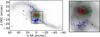 |
Fig. A.1 F814W image of NGC 2623. North is up, East is left. The detected clusters are marked with apertures of different colors corresponding to their distances with respect to the center: 1) blue clusters are those with d> 1 HLR, 2) green clusters if 0.5 HLR <d ≤ 1 HLR, and 3) red clusters if d< 0.5 HLR. In the left panel the whole galaxy is shown, where the black rectangle indicates the region simultaneously covered by all the filters from UV to NIR. A zoom into this region is shown in the right panel. |
We have roughly estimated the stellar population properties of the super star clusters (SSCs) in NGC 2623 using the HST images from FUV to NIR. According to Alvensleben (2004), a long wavelength basis from U band through NIR is necessary to determine the SP properties of star clusters in a reliable way, where the availability of U-band photometry is crucial. The characteristics of the HST images used by us are summarized in Table A.1. The methodology followed for cluster detection and aperture photometry was described in Appendix A of Cortijo-Ferrero et al. (2017).
By comparing the colors and magnitudes of NGC 2623 clusters with solar metallicity stellar population synthesis models (Charlot & Bruzual 2007, unpublished), we have derived their main properties; ages, masses, and the amount of dust obscuration. Model colors have been computed using STSDAS.SYNPHOT software.
Clusters were detected in a combination of optical HST images with IRAF DAOFIND task, and photometry performed using the phot task in APPHOT.
From 0–1 HLR there exists a strong negative AV gradient in NGC 2623 (see Fig. 5). To take into account the extinction effects with distance, we have decided to separate the clusters into three bins, according to their distances (d) to the center:
-
1.
Blue clusters: d> 1 HLR.
-
2.
Green clusters: 0.5 HLR <d ≤ 1 HLR.
-
3.
Red clusters: d< 0.5 HLR.
Basically, the blue clusters are located in the concentration of clusters south of the nucleus reported by Evans et al. (2008), while the red ones are located in the highly obscured nuclear region. Strong dust lanes can be seen in the nucleus of NGC 2623 in HST B and V band images.
A total of 156 clusters were detected with S/N> 5 in FUV, F435W, and F814W, in the region common to all filters. Similarly, 203 clusters were detected with S/N> 5 in F435W, F814W, and F160W. The clusters are shown in Fig. A.1. In the left panel, the whole galaxy is shown, where the black rectangle indicates the region simultaneously covered by all the filters from UV to NIR. A zoom into this region is shown in the right panel.
Appendix A.1: Clusters age and extinction
We have compared the colors and magnitudes of NGC 2623 clusters with those of Charlot & Bruzual SSP models (2007, unpublished) in an age range of 1 Myr to 13 Gyr. Despite the recent improvements in modeling techniques, it is very difficult to estimate the metallicity of individual clusters from photometry. From the spectroscopy we obtain an average value for the metallicity of ~0.7 Z⊙. Taking this into account, we have used the Z⊙ SSP models as a proxy in this analysis.
We can estimate the cluster ages by comparing the position of the clusters in color-color diagrams with respect to the model positions. In Fig. A.2 we show the FUV−F435W versus F435W−F814W diagram, which is the best for breaking the age −AV degeneracy. The color coding is the same as in Fig. A.1, but only those clusters with S/N ≥ 5 in FUV, F435W, and F814W filters are included in the plots. The black solid line is the path described by SSP models from 1 Myr to 13 Gyr, Z⊙, and AV = 0 mag. The gray-scale lines are the paths for the same models reddened by 1 to 3 mag, with the lighter shades tracing the more reddened models.
Similarly, in Fig. A.3 we show the F435W−F814W versus F814W−F160W diagram. Only clusters with S/N ≥ 5 in F435W, F814W, and F160W filters are shown. Again, the black solid line is the path described by SSPs from 1 Myr to 13 yr, Z⊙, and AV = 0 mag. The gray-scale lines are the paths for the same models reddened by up to 6 mag, with the lighter shades tracing the larger AV models.
From one side, the concentration of clusters south of the nucleus (d> 1 HLR) is consistent with not being affected by foreground extinction. They have ages ranging 100–400 Myr, with an average around ~250 Myr. Only a few of them could be younger if we consider them to be affected by some extinction. On the contrary, the nuclear clusters (d< 0.5 HLR) are affected by high extinction, 1–3 mag. Most of them are consistent with ages younger than 100 Myr. This suggests that the nuclear region of NGC 2623 is slightly younger than its surroundings. The greater scatter is in the circumnuclear clusters 0.5 HLR <d ≤ 1 HLR. They are consistent with an average extinction of around 1 mag. Given their spread in the diagrams they are compatible with having ages ranging 1–500 Myr. We note that the photometric estimation of the stellar population properties, although rougher, is consistent with the spectroscopic one.
Appendix A.2: Clusters masses
We found that NICMOS 1.6 μm band is the most sensitive to mass variations. We estimated the mass range of the star clusters, by comparing their 1.6 μm absolute magnitude with the absolute magnitude of SSP models of masses ranging from 104 to 108M⊙. The results are shown in Fig. A.4. This is an optical color-color versus NIR 1.6 μm absolute magnitude diagram. The paths from models of 104, 105, 106, 107, and 108M⊙ are shown as solid and dashed lines. The models have been cut between 1 and 500 Myr, as we know from the previous section that these are the oldest ages our clusters can have. We found a large range of masses in the clusters of NGC 2623. The intermediate-age clusters in the region south of the nucleus (d> 1 HLR, blue) have masses in the range 104–105M⊙. For the circumnuclear (0.5 HLR <d ≤ 1 HLR, green), the spread is larger: 104–107M⊙. On the other hand, the vast majority of the inner nuclear clusters (d< 0.5 HLR, red) are consistent with masses in the range 106–108M⊙. These impressively large masses are comparable to the most massive globular clusters seen in giant elliptical galaxies and the massive, intermediate-age clusters seen in NGC 7252 and NGC 1316 (Maraston et al. 2004; Bastian et al. 2006), and some YMC in Arp 220 (Wilson et al. 2006). We think, however, that we are not measuring masses of individual clusters, but aggregates of them.
We performed a rough estimate of the total mass in clusters in NGC 2623, by assigning a certain average mass for the clusters in each luminosity L1.6 μm range. In particular, we separated the clusters in five possible luminosity ranges: if log L1.6 μm < 0.9 we assign a mass of ~104M⊙, from 0.9 < log L1.6 μm < 1.5 we assign a mass of ~105M⊙, if 1.5 < log L1.6 μm < 2.65 then ~106M⊙, if 2.65 < log L1.6 μm < 3.5 then ~107M⊙, and above log L1.6 μm> 3.5 we assign ~108M⊙. In the case of NGC 2623 we have 39, 64, 75, 22, and 3 clusters in these respective ranges. This leads to a rough estimate of the total mass in clusters in NGC 2623 of 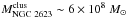 , which represents 1% of the total stellar mass.
The mass in young components derived through the IFS is comparable (only a factor ~1.5 less) to the mass in star clusters derived roughly from the photometry. This would agree with the hypothesis that the vast majority of stars form in clusters rather than in isolation.
Appendix A.3: Cluster detection limits
As explained in CF17, a major question to be addressed with star-cluster photometry is to know whether older/more reddened clusters could have been detected. We followed a simplistic approach to estimate which clusters could be, in principle, detected, and which could not. Using the SSP models of 10 Myr, 100 Myr, 200 Myr, 300 Myr, 500 Myr, and 1 Gyr, and the transmission curves from F435W and F814W filters, we compute the 435 and 814 mag for clusters of different masses (105M⊙, 106M⊙, 107M⊙, and 108M⊙) and affected by extinctions of 0 mag, 1 mag, 2 mag, 4 mag, 6 mag, and 10 mag. These magnitudes are compared with the F435W and F814W limiting magnitudes expected for point sources (most clusters are not resolved) with S/N = 5, obtained from Figure 10.2 and 10.32 of the ACS Instrument Handbook, given the exposure times of the HST observations used in this paper (~103 s).
Given the fact that NGC 2623 is nearer, but with a distance very similar to IC 1623 W (80 Mpc vs. 86.8 Mpc), the detection limits for IC 1623 W apply to NGC 2623 as well. The less massive the cluster, the more difficult it is to detect as it ages or is more reddened. Clusters of 105M⊙ up to 300 Myr can be detected for no extinction, for AV = 1 mag, while clusters older than 100 Myr cannot be detected, and for AV = 2–4 mag, only clusters of 10 Myr can be detected. 106M⊙ clusters up to 1 Gyr could be detected up to extinction levels of AV = 2 mag. For AV = 4 mag, only clusters up to 300 Myr can be detected, and for AV = 6 mag, only 10 Myr clusters can be detected. Above that extinction level, we cannot detect clusters anymore. More massive clusters, 107–108M⊙, can be detected without problems up to ages of 1 Gyr, and AV = 6 mag.
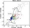 |
Fig. A.2 FUV−F435W vs. F435W−F814W diagram for NGC 2623 clusters. The color coding is the same as in Figure A.1, but only those clusters with S/N> 5 in FUV, F435W, and F814W filters are included in the plots. The black solid line is the path described by SSPs from 1 Myr to 13 Gyr, Z⊙, and AV = 0 mag. The gray-scale lines are the paths for the same models reddened by 1 to 3 mag, with the lighter shades tracing the more extincted models. |
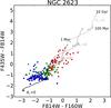 |
Fig. A.3 F435W−F814W vs. F814W−F160W diagram for NGC 2623 clusters. Only clusters with S/N> 5 in F435W, F814W, and F160W filters are shown. The black solid line is the path described by SSPs from 1 Myr to 13 Gyr, Z⊙, and AV = 0 mag. The gray-scale lines are the paths for the same models but reddened by 2, 4, and 6 mag. The clusters color coding is the same as in Fig. A.1. |
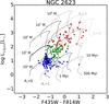 |
Fig. A.4 Right: NIC 1.6 μm absolute magnitude vs. F435W−F814W diagram. Only clusters with S/N > 5 in F435W, F814W and F160W filters are shown. The clusters color coding is the same as in Fig. A.1. The solid and dashed lines are the path of SSPs from 1 Myr to 500 Myr and with masses from 105 to 108M⊙. The gray-scale coding represents the variation in stellar extinction as in previous figures. |
Appendix B: Uncertainties related with models choice: GM vs. CB bases
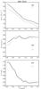 |
Fig. B.1 Comparison of the radial profiles of the stellar population properties derived with GM base (black lines) and CB base (gray lines). From top to bottom: stellar mass surface density, mean light-weighted stellar ages, and stellar dust attenuation. |
As mentioned in Sect. 3.1, we performed two sets of starlight fits using the so-called GM and CB bases. In the paper we presented the results with GM base. To take into account the uncertainties related with the model choice, here we compare the results from both bases, focusing on CALIFA data.
Cid Fernandes et al. (2014) calculate the uncertainties in the stellar population properties due to the choice of model base (GM or CB), using ~100 000 spectra from 107 galaxies observed by CALIFA. They found that the uncertainties related to the choice of base models are larger than those associated with data and method, with one-σ differences in ⟨ log age ⟩ L, AV of ~0.15 and 0.08 dex, respectively.
In Fig. C.1 we compare the radial profiles of NGC 2623 stellar population properties derived with bases GM (black) and CB (gray). From the comparison of the mass surface density profiles obtained with the two bases (top panel), we find that GM yields higher mass densities by 0.32 ± 0.08 dex, on average. This difference cannot be explained by the IMF change alone (~0.25 dex, GD15), and it is also affected by the differences in the other stellar population properties, especially the stellar ages. At distances larger than 0.5 HLR, the average difference in mass density, 0.28 ± 0.03 dex, can be explained by the IMF change. It is in the inner <0.5 HLR where the discrepancy is significantly larger, 0.47 ± 0.06 dex, coinciding with the region where the GM base starts to give older average stellar ages than CB, by 0.10 ± 0.05 dex, while outwards of 0.5 HLR it is the opposite; they are younger and more similar, −0.04 ± 0.03 dex (middle panel). The extinction derived is very similar with both bases, with GM returning only slightly higher extinctions than CB, by 0.05 ± 0.02 mag, across the whole spatial extension (bottom panel).
Thus, we conclude that when using different model bases (GM or CB) the SFH derived is slightly different, as reflected by the change in stellar ages, especially in the inner <0.5 HLR. As a consequence, the mass surface density and mass dependent quantities, such as the M/L ratio (see Fig. C.1), are somewhat larger for GM than for CB, with the difference not being solely due to the IMF change from Salpeter (GM) to Chabrier (CB).
Appendix C: Comparison of optical and NIR surface brightness profiles
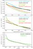 |
Fig. C.1 Top panel: comparison of the different surface brightness profiles. Middle panel: same profiles normalized at 1 HLR to compare the slopes. Bottom panel: comparison of the observed (solid green line) and dereddened (dashed green line) NIC3 F160W brightness profile, with NIC2 F160W profile reported in the literature by Scoville et al. (2000). |
In Sect. 5.5 we discuss whether NGC 2623 can evolve into an E galaxy. We compare the radial distribution of the stellar mass surface density (μ⋆) of NGC 2623 to that of non-interacting galaxies, previously obtained by GD15. We find that, globally, NGC 2623 μ⋆ is ~0.6 dex less dense than massive E galaxies, and even ~0.3 dex less dense than E/S0 of the same stellar mass. Also, the gradient in the central 1 HLR is more similar to early-type spirals. Thus, NGC 2623 is set to evolve into an Sa–Sb spiral; but we cannot rule out the possibility that it might also evolve into an E of M⋆< 1011M⊙. Because our estimation of μ⋆ depends on the M/L ratio, and this ratio depends on the stellar ages and extinction, we need to discuss whether or not our estimations of these two stellar properties can affect our conclusion.
To check if the radial distribution of μ⋆ is affected by an insufficient correction of the stellar extinction, we compare the surface luminosity profile at 1.6 μm predicted by our spectral synthesis to the one observed by NICMOS at HST. It is well known that the NIR brightness distribution is a good tracer of the stellar mass in galaxies, since it is dominated by old stars and the effect of extinction is lower at NIR than at optical wavelengths.
We use the HST NICMOS F160W image (NIC3 camera), the same as in the star cluster analysis in Appendix A, to extract the NIR surface brightness profile (green line in Fig. C.1) with the same geometric parameters as for the radial profiles of the stellar population properties derived using the PPaK continuum images. We also extract the surface brightness profile from the HST ACS F814W image (orange line in Fig. C.1).
From the SFH derived from the spectral synthesis, we have predicted the synthetic surface brightness profile at 1.6 μm (red line in Fig. C.1) using the results from the CB base7. Because at each position we have the synthetic spectrum (already corrected by extinction), we can measure from it the flux at 1.6 μm and generate an image from which the radial profile is derived.
In the top panel of Fig. C.1 we show how these NIR surface brightness profiles compare to the observed optical surface brightness (black line) and to the extinction-corrected optical surface brightness from the CALIFA datacube (blue line). It is clear that our “synthetic” radial profile at 1.6 μm is quite similar to the NIC3 F160W profile (a little brighter, as expected, since our synthetic profile is already corrected by extinction), considering the effect of the PSF in the center. In the middle panel of Fig. C.1, we show them normalized at 1 HLR in order to compare the slopes. We find that our extinction must be correct, as the slope of the de-reddened optical surface brightness profile coincides quite well with the NIC3 F160W profile, except in the PSF-affected nuclear region. This prevents us from tracing the inner steep rise of the de Vaucouleurs law with our data.
We also note that the F160W brightness profile from NIC3 is slightly shallower than the one reported in the literature with NIC2 in Scoville et al. (2000). In the bottom panel of Fig. C.1 we show how they compare. The black dashed line is the profile by Scoville et al. (2000), the green line is the profile from NIC3, and the dashed green line is the extinction-corrected profile (treated in the same way as the data in Scoville et al. 2000). We note that even the NIC3 profile seems to suffer from PSF smearing when compared to the higher-resolution NIC2 profile. Thus, we can conclude that at radial distances outside the nucleus our CALIFA mass/luminosity profiles are in good agreement with NIR estimations. In the nuclear regions the CALIFA data are limited by the spatial resolution of PPaK with respect to NIC2.
With respect to the stellar ages, its effect is already discussed in Appendix B and shown in Fig. C.1, where we compare μ⋆ and ⟨ log age ⟩ L derived from GM and from CB. Due to the change of IMF, μ⋆ is a factor 1.8 higher with GM than with CB. Also, due to some differences in the SFH derived with the two sets of SSPs, the stellar ages derived with GM are older than those derived with CB. As a consequence, GM fits provide a higher M/L ratio in the central 0.5 HLR of NGC 2623, and a gradient ~0.3 dex steeper. We note that these are intrinsic uncertainties associated to the analysis which we cannot break.
In anycase, we find that the M/L5635 (GM) values derived by us (Fig. C.2) are in good agreement with the ones expected from the M/Lg and M/Lr calibrations provided by Bell et al. (2003) assuming (g−i) = 1.1, which is the SDSS color of NGC 2623;
or (g−i) = 0.86 if the color is corrected by an average extinction of AV = 0.5 mag. These expressions by Bell et al. (2003) were computed assuming an exponentially declining SFR, and a Salpeter IMF. Further, our M/L5635 results for NGC 2623 are also in the range of expected values for Sbc–Sc galaxies in the CALIFA sample (García-Benito et al., in prep.).
However, the M/L at 1.6 μm, derived by the ratio between the radial profile of μ⋆ (CB) and the NIC3 surface brightness profile at 1.6 μm and between μ⋆ (CB) and the 1.6 μm synthetic radial profile are a factor ~4 and ~2 higher, respectively, with respect to the 0.5 (M⊙/L⊙) value expected for a Chabrier IMF (Zibetti et al. 2009). The origin of this discrepancy is not clear for us, but its investigation is beyond the scope of this paper.
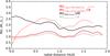 |
Fig. C.2 Radial profile of M/L5635 derived from the ratio between μ⋆ and L5635 (the luminosity measured at the normalized wavelength corrected by the stellar extinction) obtained for GM (black) and CB (grey) bases. M/L at the observed 1.6 μm and at the synthetic 1.6 μm are shown as dashed-red and solid-red lines, respectively. |
All Tables
All Figures
|
Fig. 1 Top panel: HST ACS F555W image of NGC 2623. The black rectangle indicates the FoV covered by the LArr IFS, while the black hexagon indicates PPaK FoV. Lower left panel: continuum flux at 5110 Å rest-frame (obtained by averaging the spectra in the range 5050–5170 Å), Fλ5110, for the CALIFA data. Lower right panel: Fλ5110 for LArr data. |
| In the text | |
|
Fig. 2 Left panel: HST F435W continuum image of NGC 2623, with the average continuum from CALIFA IFS superimposed using red contours. Several regions of the galaxy are labelled. Right panel: spectra from different regions extracted in circular apertures of 2′′ radius, in black the PPaK nuclear spectrum, in red the LArr nuclear spectrum, and in blue the spectrum from the cluster-rich region to the south of the nucleus. The spectra are normalized by the flux at 5500 Å, and an offset is applied to better visualize the differences. |
| In the text | |
|
Fig. 3 Integrated CALIFA spectrum for NGC 2623 normalized at 5500 Å, in the Hα + [NII] region. The OSIRIS TF narrow-band filter bandpasses at the galaxy center are shown in red, while the positions of the filters at the location of the star forming regions (R1 to R4, see Sect. 4.7) are shown in blue. |
| In the text | |
|
Fig. 4 Upper left: CALIFA map of the stellar mass surface density (μ⋆). The white dashed lines indicate the position of 1, 2, and 3 half-light radii (HLR); 1 HLR is equivalent to 2.8 kpc in physical distance. The contours correspond to the smoothed HST F555W image. Upper right: LArr map of stellar mass surface density. The color-scale is the same as for the CALIFA map. Below is presented a zoom of the CALIFA map in the nuclear region, to match the region covered by LArr map. Lower panel: radial profile of log μ⋆ as a function of the radial distance in HLR (lower horizontal axis) and kpc (upper horizontal axis), in red for LArr and black for CALIFA. The uncertainties, calculated as the standard error of the mean, are shaded in light red and gray, respectively. For comparison, the gray lines are the profiles from Sbc (solid) and Sc (dashed) spiral galaxies from CALIFA (González Delgado et al. 2015), with stellar masses similar to that of NGC 2623. We also include the profiles of the early-stage mergers IC 1623 W (blue), NGC 6090 NE (orange), and NGC 6090 SW (green). |
| In the text | |
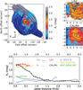 |
Fig. 5 As in Fig. 4 but for stellar dust extinction. |
| In the text | |
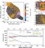 |
Fig. 6 As in Fig. 4 but for mean light-weighted stellar ages. |
| In the text | |
|
Fig. 7 Left panels: percentage contributions of young t< 140 Myr, intermediate (140 Myr <t< 1.4 Gyr) and old t> 1.4 Gyr stellar populations to the observed light at 5635 Å. Right panel: radial profiles of the light contributions from young xY (blue), intermediate xI (green) and old populations xO (red) with the radial distance in HLR and kpc. For comparison, the dashed lines with the same colors are the profiles for Sbc spiral galaxies from CALIFA. |
| In the text | |
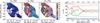 |
Fig. 8 As in Fig. 7 but for contributions to stellar mass. |
| In the text | |
|
Fig. 9 OSIRIS Hα (left) and CALIFA Hα (right) emission line fluxes in units of 10-16 erg s-1 cm-2 arcsec-2 presented on a logarithmic scale. The black cone delimits the nuclear outflowing nebula reported by Lípari et al. (2004). The HST F555W image is shown in contours, smoothed to approximately match the spatial resolution of our IFS data. |
| In the text | |
|
Fig. 10 Zoom of the OSIRIS Hα emission line image for the nuclear region of NGC 2623. HST continuum contours are overplotted in black. The black dot marks the continuum center. |
| In the text | |
|
Fig. 11 HST F555W continuum image of the nuclear region of NGC 2623 together with the OSIRIS Hα line emission plotted as red contours. The star cluster aggregations, A and B, and the HII regions, C1, C2, and C3 are labelled. The positions of the Hα lobe and SF associated to the tip of the lobe are also marked. |
| In the text | |
|
Fig. 12
|
| In the text | |
|
Fig. 13 Left: emission line ratio map of [NII]λ6584/Hα derived from the OSIRIS data. The box in the lower left corner is a zoom of the nuclear region. Right: [NII]λ6584/Hα derived from the CALIFA data. |
| In the text | |
|
Fig. 14 [NII]λ6584/Hα vs. [OIII]λ5007/Hβ (left panel), and [OI]λ6300/Hα vs. [OIII]λ5007/Hβ (right panel) line ratio diagnostic diagrams. Spaxels are color-coded according to the Hα velocity dispersion map shown in Fig. 15. Solid lines in both diagnostic diagrams mark the “maximum starburst lines” obtained by Kewley et al. (2001, K01) by means of photoionization models of synthetic starbursts; the dotted line in the left panels marks the pure SDSS star-forming galaxies frontier semi-empirically drawn by Kauffmann et al. (2003, K03); and the dashed-dotted lines that separate Seyferts from LINERs are from Cid Fernandes et al. (2010, CF10) and Kewley et al. (2006, K06). The average error bars are shown in the top-left corners. |
| In the text | |
|
Fig. 15 Top panel: velocity dispersion derived from Hα, corrected for the instrumental width (σinst ~ 116 km s-1). Bottom panel: velocity field derived from Hα. The position angles of the kinematic major axis for the approaching and receding sides have been calculated by Barrera-Ballesteros et al. (2015) and are shown in the figure with black solid lines. The circle in the top right corner of both maps represents the spatial resolution, given by the diameter of PPaK fibres, ~2.7′′. |
| In the text | |
|
Fig. 16 OSIRIS ~6723 Å map emission flux image derived from the OSIRIS data. This corresponds to the [NII]λ6584 rest frame at the NGC 2623 center, and to between [NII]λ6548 and Hα emission in R1, R2, R3, and R4. |
| In the text | |
|
Fig. 17 Radial profile of log μ⋆ for NGC 2623 (black line) and for a sub-sample of E/S0 and spiral galaxies from the CALIFA survey that have a stellar mass (10.5 ≤ log M⋆ (M⊙) ≤ 10.9) similar to NGC 2623. |
| In the text | |
|
Fig. A.1 F814W image of NGC 2623. North is up, East is left. The detected clusters are marked with apertures of different colors corresponding to their distances with respect to the center: 1) blue clusters are those with d> 1 HLR, 2) green clusters if 0.5 HLR <d ≤ 1 HLR, and 3) red clusters if d< 0.5 HLR. In the left panel the whole galaxy is shown, where the black rectangle indicates the region simultaneously covered by all the filters from UV to NIR. A zoom into this region is shown in the right panel. |
| In the text | |
|
Fig. A.2 FUV−F435W vs. F435W−F814W diagram for NGC 2623 clusters. The color coding is the same as in Figure A.1, but only those clusters with S/N> 5 in FUV, F435W, and F814W filters are included in the plots. The black solid line is the path described by SSPs from 1 Myr to 13 Gyr, Z⊙, and AV = 0 mag. The gray-scale lines are the paths for the same models reddened by 1 to 3 mag, with the lighter shades tracing the more extincted models. |
| In the text | |
|
Fig. A.3 F435W−F814W vs. F814W−F160W diagram for NGC 2623 clusters. Only clusters with S/N> 5 in F435W, F814W, and F160W filters are shown. The black solid line is the path described by SSPs from 1 Myr to 13 Gyr, Z⊙, and AV = 0 mag. The gray-scale lines are the paths for the same models but reddened by 2, 4, and 6 mag. The clusters color coding is the same as in Fig. A.1. |
| In the text | |
|
Fig. A.4 Right: NIC 1.6 μm absolute magnitude vs. F435W−F814W diagram. Only clusters with S/N > 5 in F435W, F814W and F160W filters are shown. The clusters color coding is the same as in Fig. A.1. The solid and dashed lines are the path of SSPs from 1 Myr to 500 Myr and with masses from 105 to 108M⊙. The gray-scale coding represents the variation in stellar extinction as in previous figures. |
| In the text | |
|
Fig. B.1 Comparison of the radial profiles of the stellar population properties derived with GM base (black lines) and CB base (gray lines). From top to bottom: stellar mass surface density, mean light-weighted stellar ages, and stellar dust attenuation. |
| In the text | |
|
Fig. C.1 Top panel: comparison of the different surface brightness profiles. Middle panel: same profiles normalized at 1 HLR to compare the slopes. Bottom panel: comparison of the observed (solid green line) and dereddened (dashed green line) NIC3 F160W brightness profile, with NIC2 F160W profile reported in the literature by Scoville et al. (2000). |
| In the text | |
|
Fig. C.2 Radial profile of M/L5635 derived from the ratio between μ⋆ and L5635 (the luminosity measured at the normalized wavelength corrected by the stellar extinction) obtained for GM (black) and CB (grey) bases. M/L at the observed 1.6 μm and at the synthetic 1.6 μm are shown as dashed-red and solid-red lines, respectively. |
| In the text | |
Current usage metrics show cumulative count of Article Views (full-text article views including HTML views, PDF and ePub downloads, according to the available data) and Abstracts Views on Vision4Press platform.
Data correspond to usage on the plateform after 2015. The current usage metrics is available 48-96 hours after online publication and is updated daily on week days.
Initial download of the metrics may take a while.