| Issue |
A&A
Volume 594, October 2016
|
|
|---|---|---|
| Article Number | A37 | |
| Number of page(s) | 19 | |
| Section | Galactic structure, stellar clusters and populations | |
| DOI | https://doi.org/10.1051/0004-6361/201628559 | |
| Published online | 07 October 2016 | |
Photoionization models of the CALIFA H II regions
I. Hybrid models
1 Instituto de Astronomía, Universidad Nacional Autonoma de Mexico, Apdo. Postal 70264, 04510 Mexico D.F., Mexico
e-mail: This email address is being protected from spambots. You need JavaScript enabled to view it.
2 Millennium Institute of Astrophysics, Chile
3 Departamento de Astronomía, Universidad de Chile, Camino El Observatorio 1515, Las Condes, Santiago, Chile
4 Instituto de Astrofísica de Andalucía (CSIC), Glorieta de la Astronomía s/n, Aptdo. 3004, 18080 Granada, Spain
5 European Southern Observatory (ESO), Karl-Schwarzschild-Str.2, 85748 Garching b. München, Germany
6 Department of Physics, Institute for Astronomy, ETH Zürich, 8093 Zürich, Switzerland
7 Departamento Astrofísica, Universidad Complutense de Madrid, Avda. Ciudad Universitaria s/n, 28040 Madrid, Spain
8 Leibniz Institut für Astrophysik, An der Sternwarte 16, 14482 Potsdam, Germany
Received: 20 March 2016
Accepted: 3 June 2016
Abstract
Photoionization models of H ii regions require as input a description of the ionizing spectral energy distribution (SED) and of the gas distribution, in terms of ionization parameter U and chemical abundances (e.g., O/H and N/O).A strong degeneracy exists between the hardness of the SED and U, which in turn leads to high uncertainties in the determination of the other parameters, including abundances. One way to resolve the degeneracy is to fix one of the parameters using additional information. For each of the ~20 000 sources of the CALIFA H ii regions catalog, a grid of photoionization models is computed assuming the ionizing SED to be described by the underlying stellar population obtained from spectral synthesis modeling. The ionizing SED is then defined as the sum of various stellar bursts of different ages and metallicities. This solves the degeneracy between the shape of the ionizing SED and U. The nebular metallicity (associated with O/H) is defined using the classical strong line method O3N2 (which gives our models the status of “hybrids”). The remaining free parameters are the abundance ratio N/O and the ionization parameter U, which are determined by looking for the model fitting [N ii]/Hα and [O iii]/Hβ. The models are also selected to fit [O ii]/Hβ. This process leads to a set of ~3200 models that reproduce the three observations simultaneously. We find that the regions associated with young stellar bursts (i.e., ionized by OB stars) are affected by leaking of ionizing photons,the proportion of escaping photons having a median of 80%. The set of photoionization models satisfactorily reproduces the electron temperature derived from the [O iii]λ4363/5007 line ratio. We determine new relations between the nebular parameters, like the ionization parameter U and the [O ii]/[O iii] or [S ii]/[S iii] line ratios. A new relation between N/O and O/H is obtained, mostly compatible with previous empirical determinations (and not with previous results obtained using photoionization models). A new relation between U and O/H is also determined. All the models are publicly available on the Mexican Million Models database 3MdB.
Key words: ISM: abundances / ISM: general / Hii regions / local insterstellar matter
© ESO, 2016
1. Introduction
Classical H ii regions are large, low-density clouds of partially ionized gas in which star formation has recently taken place (<15 Myr). The short-lived blue stars forged in these regions emit large amounts of ultraviolet radiation that ionizes the surrounding gas. They span a wide range of physical scales from a few parsecs, like the Orion nebula (D ~ 8 pc) or even smaller (Anderson 2014), to hundreds of parsecs, such as 30 Doradus (D ~ 20 pc), NGC 604 (D ~ 460 pc), or NGC 5471 (D ~ 1 kpc) as reported by Oey et al. (2003) and García-Benito et al. (2011). These last examples are the prototypes of the extragalactic giant H ii regions found frequently in the disks of spiral galaxies (e.g., Hodge & Kennicutt 1983; Dottori 1987; Dottori & Copetti 1989; Knapen 1998), or starburst and blue compact galaxies (e.g., Kehrig et al. 2008; López-Sánchez & Esteban 2009; Cairós et al. 2012).
Baldwin et al. (1981) first proposed the [O iii]λ5007/Hβ versus [N ii]λ6584/Hα diagnostic diagram (now known as the BPT diagram) to separate emission-line objects according to the main gas excitation mechanism: normal H ii regions, planetary nebulae, and objects photoionized by a harder radiation field. The lastcan be produced by either a power-law continuum from an active galactic nucleus (AGN), shock excitation, planetary nebulae central stars, or even post-asymptotic giant branch (AGB) stars (e.g., Binette et al. 1994, 2009; Stasińska et al. 2008; Morisset & Georgiev 2009; Flores-Fajardo et al. 2009; Kehrig et al. 2012; Singh et al. 2013; Papaderos et al. 2013). Veilleux & Osterbrock (1987) and Osterbrock (1989) extended and refined this classification scheme, incorporating new diagnostic diagrams. Osterbrock (1989) used theoretical photoionization models to infer the demarcation line between star forming (SF) and AGN galaxies, and added two new diagnostics diagrams that exploit the [O i]/Hβ versus [S ii]/Hα line ratios. Dopita et al. (2000) and Kewley et al. (2001) combined stellar population synthesis and photoionization models to build the first purely theoretical classification scheme for separating pure AGNs from galaxies hosting star formation, and Kauffmann et al. (2003) used Sloan Digital Sky Survey (SDSS York et al. 2000) data to observationally constrain these classifications.
In essence, these models assume that the main factors that control the emission line spectrum are the chemical abundances of the heavy elements in the gas phase within an H ii region (oxygen being the most important), the shape of the ionizing radiation spectrum, and the geometrical distribution of gas with respect to the ionizing sources. Generally speaking, all the geometrical factors are subsumed into a single factor, the ionization parameter q (with dimensions cm s-1), or the (dimensionless) ionization parameter U = q/c. They also assume a priori that these parameters are independent, and thus these models are presented as grids of oxygen abundance, ionization parameter, shape of the ionizing spectrum (effective temperature or stellar burst age), and sometimes electron densities.
Most of the present day knowledge of these regions is based on the comparison of the predictions between these photoionization models and the largest accessible databases for the observed properties of H ii regions. However, in many cases, the samples/catalogs are limited in number (a few hundred of H ii regions) and/or biased (H ii hosted by Sc/Sd galaxies due to the better contrast with the continuum). This has recently been overcome by the advent of large IFU surveys that have provided large catalogs of H ii regions/aggregations with spectroscopic information (on the order of thousands) over an unbiased sample of galaxies (from E to Sds; see, e.g., Marino et al. 2016; Sánchez-Menguiano et al. 2016).
This is the case of the Calar Alto Legacy Integral Field spectroscopy Area survey (CALIFA) survey (Sánchez et al. 2012b), which has acquired Integral Field Unit (IFU) data of a sample of ~600 galaxies in the Local Universe (0.005 <z< 0.03) covering the full optical extension of these galaxies (see Walcher et al. 2014, for more information on the sample). This survey has created one of the largest catalogs of H ii regions/aggregations, with more than 20 000 ionized regions, with spectroscopic information covering most of the typical emission lines in the optical wavelength range from [O ii]λ3727 to [S ii]λ6731, and with an accurate spectral modeling and subtraction of the underlying stellar population.
One of the main problems in the determination of the properties of HII regions is that some of the parameters that describe these properties act in very similar ways on the observations. This is the case for the softness of the ionizing radiation and the ionization parameter U. Both change the ionization state of the nebula, in particular the line ratios involving two subsequent ions (e.g., [O ii]/[O iii]). The best way to resolve this degeneracy is to find a method for determining one of the two parameters using an alternative observable. Combining the output from spectral synthesis modeling of the CALIFA observations gives us access to the softness of the ionization field, leaving only U to be determined.
In this article we use this extensive catalog to create an ad hoc grid of photoinization models, with the properties of the ionizing sources a priori provided by the analysis of the stellar populations, in order to understand the physical conditions of these nebulae. We also use an a priori determination of the O/H metallicity indicator (using a strong line method) to only have the ionization parameter U and the N/O abundance ratio as free parameters. We are actually doing work similar to Pérez-Montero et al. (2010), but are using a much larger set of observations.
The paper is organized as follows: Sect. 2 describes the CALIFA data set used in this work. The grids of models (meta-grid and ad hoc models for each region) are described in Sect. 3. The results are presented and discussed in Sect. 4, and the conclusions are drawn in Sect. 5.
2. CALIFA data
The galaxies were selected from the CALIFA observed sample. Since CALIFA is an ongoing survey whose observations are scheduled on a monthly basis (i.e., on dark nights), the list of objects increases regularly. The current results are based on the 612 galaxies observed up to June 2014, comprising galaxies from the CALIFA mother sample and the so-called extended sample (details in Sánchez et al. 2016a). Their main characteristics have already been described in Sánchez et al. (2015).
The details of the survey, sample, observational strategy, and reduction are explained in Sánchez et al. (2012a). All galaxies were observed using PMAS (Roth et al. 2005) in the PPAK configuration (Kelz et al. 2006), covering a hexagonal field of view (FoV) of 74″× 64″, which is sufficient to map the full optical extent of the galaxies up to two to three disk effective radii. This is possible because of the diameter selection of the sample (Walcher et al. 2014). The observing strategy guarantees complete coverage of the FoV with a final spatial resolution of FWHM ~ 2.5″ (García-Benito et al. 2015), corresponding to ~1 kpc at the average redshift of the survey. The sampled wavelength range and spectroscopic resolution (3745 Å−7500 Å, λ/ Δλ ~ 850, for the low-resolution setup) are more than sufficient to explore the most prominent ionized gas emission lines from [O ii]λ3727 to [S ii]λ6731 at the redshift of our targets on the one hand, and to deblend and subtract the underlying stellar population on the other (e.g., Sánchez et al. 2012a; Kehrig et al. 2012; Cid Fernandes et al. 2013, 2014). The data set was reduced using version 1.5 of the CALIFA pipeline, whose modifications with respect to those presented in Sánchez et al. (2012a) and Husemann et al. (2013) are described in detail in García-Benito et al. (2015). In summary, the data fulfill the predicted quality-control requirements with a spectrophotometric accuracy that is better than 5% everywhere within the wavelength range, both absolute and relative, with a depth that allows us to detect emission lines in individual H ii regions as faint as ~10-17 erg s-1 cm-2 and with a signal-to-noise ratio of S/N ~ 3−5. For the emission lines considered in the current study, the S/N is well above this limit, and the measurement errors are negligible in most of the cases. In all cases, they have been propagated and included in the final error budget.
The final product of the data reduction is a regular-grid datacube, with x and y coordinates that indicate the right ascension and declination of the target, and z is a common step in wavelength. The CALIFA pipeline also provides the propagated error cube, a proper mask cube of bad pixels, and a prescription of how to handle the errors when performing spatial binning (due to covariance between adjacent pixels after image reconstruction). These datacubes, together with the ancillary data described in Walcher et al. (2014), are the basic starting points of our analysis.
2.1. H II regions: detection and extraction
The segregation of H ii regions and the extraction of the corresponding spectra is performed using a semi-automatic procedure named HIIexplorer1. The procedure is based on some basic assumptions: (a) H ii regions are peaky and isolated structures with a strong ionized gas emission, which is significantly above the stellar continuum emission and the average ionized gas emission across the galaxy. This is particularly true for Hα because (b) H ii regions have a typical physical size of about a hundred or a few hundred parsecs (e.g., González Delgado & Perez 1997; Lopez et al. 2011; Oey et al. 2003), which corresponds to a typical projected size of a few arcsec at the distance of the galaxies.
These assumptions are based on the fact that most of the Hα luminosity observed in spiral and irregular galaxies is a direct tracer of the ionization of the interstellar medium (ISM) by the ultraviolet (UV) radiation produced by young high-mass OB stars. Since only high-mass, short-lived stars contribute significantly to the integrated ionizing flux, this luminosity is a direct tracer of the current star formation rate (SFR), independent of the previous star formation history. Therefore, clumpy structures detected in the Hα intensity maps are most probably associated with classical H ii regions (i.e., those regions for which the oxygen abundances have been calibrated).
The details of HIIexplorer are given in Sánchez et al. (2012b) and Rosales-Ortega et al. (2012). In summary we create a narrow-band image centered on the wavelength of Hα at the redshift of the object. Then we run HIIexplorer to detect and extract the spectra of each individual H ii region, adopting the parameters presented in Sánchez et al. (2014). The algorithm starts looking for the brightest pixel in the map. Then, the code aggregates the adjacent pixels until all pixels with flux greater than 10% of the peak flux of the region and within 500 pc or 3.5 spaxels from the center have been accumulated. The distance limit takes the typical size of H ii regions of a few hundreds of parsecs into account (e.g., González Delgado & Perez 1997; Lopez et al. 2011). Then, the selected region is masked and the code keeps iterating until no peak with flux exceeding the median Hα emission flux of the galaxy is left. Mast et al. (2014) studied the loss of resolution in IFS using nearby galaxies observed by PINGS (PPAK ISF Nearby Galaxies Survey, see Rosales-Ortega et al. 2010). Some of these galaxies were simulated at higher redshifts to match the characteristics and resolution of the galaxies observed by the CALIFA survey. Regarding the H ii region selection, the authors conclude that at z ~ 0.02, the H ii clumps can contain on average from 1 to 6 of the H ii regions obtained from the original data at z ~ 0.001. Another caveat is that this procedure tends to select regions with similar sizes, although real H ii regions actually have different sizes. However, the actual adopted size is close to the FWHM (2.5″) of the CALIFA data for the version of the data reduction we used (García-Benito et al. 2015).
Then, for each individual extracted spectrum we modeled the stellar continuum using FIT3D2, a fitting package described in Sánchez et al. (2006, 2011, 2016b). This fitting tool performs multiple linear regressions to derive the optimal combination of a single-stellar population (SSP) library over a set of Monte Carlo realizations of the input spectrum, and gives the best fitting set of weights for each population and the corresponding errors. Prior to this analysis the procedure derives the best kinematics and dust attenuation for each fitted spectrum. In this particular study we use the gsd156 template library, described in detail by Cid Fernandes et al. (2013). It comprises 156 templates that cover 39 stellar ages (1 Myr to 13 Gyr), and 4 metallicities (Z/Z⊙ = 0.2, 0.4, 1, and 1.5). These templates were extracted from a combination of the synthetic stellar spectra from the GRANADA library (Martins et al. 2005) and the SSP library provided by the MILES project (Sánchez-Blázquez et al. 2006; Vazdekis et al. 2010; Falcón-Barroso et al. 2011). This library has been extensively used within the CALIFA collaboration in different studies (e.g., Pérez et al. 2013; Cid Fernandes et al. 2013; González Delgado et al. 2014). The only difference with respect to these studies is that the spectral resolution of the library was not fixed to the spectral resolution of the CALIFA V500 setup data (FWHM ~ 6 Å) to allow its use for data sets with different resolution. As shown in Sánchez et al. (2016b) the results are not strongly affected by the selection of a different stellar template. The reliability of the derived parameters for the stellar population using FIT3D was extensively tested against simulations and perturbed data. In particular it was found that it is required a S/N above 50 to break the well-known degeneracies and provide reliable weights for the stellar population when they contribute to at least ~5% of the total flux in the visible range (e.g., Sánchez et al. 2016b, Figs. 9 and 15). In previous articles (Sánchez et al. 2014) we explored the correspondence between the estimated fraction of young stars (fy) and the equivalent width of Hα (EWα), parameters that show a clear correlation when the fy> 20% and EWα> 6 Å. This is indeed a good test that supports the reliability of the derived fraction of young stars.
After subtracting the underlying stellar population, the flux intensity of the strong emission lines was extracted for each gas-pure spectrum by fitting a single Gaussian modelto each line, resulting in a catalog of the emission-line properties (Sánchez et al. 2012b).
The final catalog comprises the strongest emission line and emission line ratios from [O ii]λ3727 to [S ii]λ6731 for 18178 H ii regions from 612 galaxies, together with their equivalent widths and the luminosity-weighted ages and metallicities of the underlying stellar population. To date, this is the largest catalog of H ii regions and aggregations with spectroscopic information. It is also one of the few catalogs derived for a statistically well-defined sample of galaxies representative of the entire population of galaxies in the local Universe (Walcher et al. 2014).
In this work, we will only use the HI, [N ii], [O ii], and [O iii]3 emision lines, which are present in almost all the sources. Auroral lines are seen only in about ten of them (see the 16 [O iii]λ4363 lines used by Marino et al. 2013).
3. Grid of models
3.1. Meta-grid
For each H ii region of each galaxy we run a grid of 220 photoionization models using the Cloudy code (Ferland et al. 2013, c13.03) driven by the pyCloudy package4 (Morisset 2013, 2014). The grids are obtained by varying the mean ionization parameter  5 which takes 11 values from −4 to −1.5, the abundance ratio log(N/O) (5 values from −1.5 to 1.5 around the solar value), the morphology parameter fr (0.03 and 3.0, see below), and the nebular metallicity (“Neb” and “Stel”, see below). Following Stasińska et al. (2015), the desired value of is obtained by setting the H0-ionizing photons emission rate Q(H0) to
 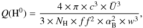 (1)where c is the speed of light, NH is the hydrogen density (set to 10 H/cm3 for all the models), ff is the filling factor, αB is the effective case B recombination coefficient, and w = (1 + fr3)1 / 3−fr with the morphology factor fr = Rin/RStr being the ratio between Rin, the inner radius of the nebula, and RStr, the Strömgren radius of the nebula if it were a full filled sphere. A morphology factor fr ≫ 1 (w ~ 0 ) corresponds to a thin shell (e.g., a plan-parallel model), while fr ~ 0 (w ~ 1 ) corresponds to a filled sphere. The Strömgren radius of a filled sphere is
 ![Mathematical equation: \begin{equation} R_{\rm Str} = \left[\frac{3 \times Q({\rm H}^0)}{4 \times \pi \times N_{\rm H}^2 \times \alpha_{\rm B} \times ff}\right]^{1/3}\cdot\nonumber \end{equation}](/articles/aa/full_html/2016/10/aa28559-16/aa28559-16-eq57.png) (2)The ionizing SED is obtained by summing up individual models from POPSTAR code (Mollá et al. 2009). Each model corresponds to an individual burst of age and metallicity from the gsd156 template and has a weight given by the multi-SSP analysis described above. We use POPSTAR models obtained following the IMF from Salpeter (1955). We checked that using an IMF from Chabrier (2003) does not significantly change our results.
(2)The ionizing SED is obtained by summing up individual models from POPSTAR code (Mollá et al. 2009). Each model corresponds to an individual burst of age and metallicity from the gsd156 template and has a weight given by the multi-SSP analysis described above. We use POPSTAR models obtained following the IMF from Salpeter (1955). We checked that using an IMF from Chabrier (2003) does not significantly change our results.
The oxygen abundance of the ionized gas is determined in two ways:
-
Neb: from the nebular [O iii]/[N ii] lineratios applying the O(O3N2) relation determined by Marinoet al. (2013,,namely 12 + log (O / H) = 8.533−0.214 × O3N2, where O3N2 is log (([O iii]/Hβ)/([N ii]/Hα));
-
Stel: the luminosity-weighted log metallicity of the underlying young stellar population, derived by co-adding the metallicities of the corresponding SSPs within the library multiplied by its contributed fraction of light in the V-band, but only for those SSPs with ages younger than 2 Gyr, following González Delgado et al. (2014). This set of models is not used in the following main analysis as we know that this determination of the nebular metallicity is less reliable owing to the low S/N of the underlying continuum for a fraction of the H ii regions (Sánchez et al. 2016b). Although the continuum has a good S/N (~30−50) to perform a SSP decomposition, to derive the metallicity of the young stars a similar S/N for only the young component is needed, which may contribute between 100% and 20% of the total flux. This cannot be granted in general. Therefore, the estimated metallicities would have large errors. The results obtained with these models are discussed in Sect. 4.8 and are shown in the Appendix A. This method has been calibrated for H ii regions and may not apply for regions ionized by old stars.
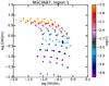 |
Fig. 1 Modeled BPT diagram [O iii]/Hβ vs. [N ii]/Hα used to interpolate the values of |
The element abundances follow O/H (except N/H which is a free parameter). The abundances relative to O are taken from Asplund et al. (2009).
Dust is included in the model, in the form of the “ism” type defined by Cloudy, with a dust-to-gas ratio following a broken power law, as in the case XCO,Z defined and recommended by Rémy-Ruyer et al. (2014). Following Draine (2011), we apply an additional factor of 2/3 to the final dust-to-gas ratio used.
The models of this meta-grid (grid of grids) are run in a quick mode (no iteration, no level-2 lines; see Cloudy manual). The ad hoc models (see next section) do not have these limitations.
Not all the CALIFA regions have been used; we apply a filter to select only the ones where the values of the CALIFA field ratio med_flux/StdDev are over 10 for the lines of interest (which corresponds to the average S/N from blue to red through the full spectral range) and the value of the CALIFA field MIN_CHISQ is over 0.7 (the reduced chi2 parameter). Both cuts ensure that the fitting provides reliable results. A total of 397 galaxies have been used, summing up 9181 regions corresponding to 2 019 820 individual photoionization models.
The models have been stored in the unpublished working database associated with 3MdB (Mexican Million Models database; see Morisset et al. 2015).
3.2. Ad hoc models
We use the meta-grid to find the model that most accurately reproduces the observed line ratios [O iii]/Hβ and [N ii]/Hα for each region. Figure 1 gives an example of the results for region 1 of NGC3687. The figure shows the classical BPT diagram, [O iii]/Hβ versus [N ii]/Hα (Baldwin et al. 1981). The blue diamond corresponds to the observed line ratios, whereas the colored circles (triangles) are the results of the grid of models obtained with fr being 0.03 (3.0), using the SED corresponding to this region and the nebular metallicity derived from the O3N2 diagnostic (see Sect. 3.1).
We have performed a 2D interpolation in the BPT diagram to determine the and the N/O ratio for each of the models. The metallicity method (Stel or Neb; see Sect. 3.1) and the geometry (fr) both take two values and thus, we obtained four ad hoc models for each region. As no extrapolation is done in the BPT diagrams, for some regions fewer than four ad hoc models are performed. The final number of ad hoc models is 20 793 (from 272 galaxies), from which 10 196 are Neb models (obtained using the O3N2 method to determine O/H).
All the 20 793 ad hoc models are stored in the 3MdB database (Morisset et al. 2015) and are accessible for any user under the “CALIFA_ah” reference (the “ref” field). The “com5” field is used to store the value of the fit for the [O ii]/Hβ/ line ratio, see Sect. 3.3. The “com8” field is used to store the result of the BPT-Population filter, see Sect. 3.6. Once the final release of the CALIFA data becomes publicly available, we plan to rerun all the procedures to obtain more data points and to store the corresponding new models in 3MdB under the “CALIFA_ah2” reference.
3.3. [O ii]/Hβ filter
The ad hoc models have been designed to fit the [N ii]/Hα and [O iii]/Hβ line ratios, but we can also impose that they fit the observed [O ii]/Hβ line ratio. We filter the models for which the value of log ([O ii]/Hβ) equals the observed value within 0.1 dex. This reduces the number of models by a factor of ~ 6, but provides us with a more realistic reference data set. To apply this filter we corrected the [O ii] line intensities from the reddening, using Hα/Hβ = 2.85 and the (Fitzpatrick 1999) extinction law. The number of ad hoc models that also fit this [O ii]/Hβ filter is 3195, of which 1574 are Neb models. In the 3MdB database, it is possible to selectthe models that fit the [O ii]/Hβ line ratio by using the “com5” entry, which contains log([O ii]/Hβ)obs −log ([O ii]/Hβ)mod.
This filter certainly adds some bias to our sample, as only 1/6 of the models remain.
We note that other emission line ratios could also be used to filter models, but they all involve abundance ratios that are not free parameters in our modeling process (e.g., using [S iii]/Hβ depends on the S/H abundance ratio). In other words, not fitting the observed [S iii]/Hβ ratio for a given observation may only indicate that the S/H abundance is not correct; however, S/H is determined by fixing S/O, and we have no way to act on [S iii]/Hβ ratio. An incorrect value for S/H has virtually no consequences on the results presented in the following sections, but would artificially exclude “good” models if we use the [S iii]/Hβ ratio as a filter.
3.4. Characterizing the ionizing population
From the study by Morisset et al. (2015), we can define limits in an age–metallicity plane for the ionizing stellar populations. Using their Fig. 5, we can determine that – for log (O / H) < −3.5 – OB stars correspond to log(age/yr) < 6.8 and HOLMES6 correspond to log(age/yr) > 8.25. For log (O / H) > −3.5, OB stars correspond to log(age/yr) < 6.7 and HOLMES correspond to log(age/yr) > 7.9. Using these limits and the decomposition of the spectra on the gsd156 library base, we can define the proportion of the ionizing photons coming from OB stars in the total number of ionizing photons Q(H0). This proportion is denoted f(OB) in the rest of the paper. There is a strong correlation between the type of dominant ionizing stellar population depicted by this f(OB) and the value of Q0 / 1 = Q(H0)/Q(He0), the ratio of the number of photons ionizing H0 and He0 (a kind of softness parameter). This is illustrated by Fig. 2, where the histograms of Q0 / 1 obtained for OB stars and HOLMES are compared. There is a clear separation at a value of ~ 0.55, HOLMES being associated with the lowest values. In the following we mainly use the Q0 / 1 ratio to trace the underlying population, keeping in mind that the purple/bluish dots point to HOLMES and the gray/reddish/yellow dots to OB stars for all figures throughout this article.
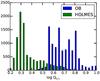 |
Fig. 2 Values of Q0 / 1 = Q(H0)/Q(He0) for the OB and HOLMES dominated spectra. |
3.5. Hα equivalent width
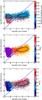 |
Fig. 3 Comparison between the EWα from the models and from the observations. Colors represent Kdist, the distance to the Kauffmann et al. (2003) curve (upper panel), the OB stars proportion f(OB) (middle panel), and the ratio Q0 / 1 = Q(He0)/Q(H0) (lower panel). The solid blue line follows y = x. In the upper panel, the solid black curves enclose half of the models that are below the Kauffman curve (negative Kdist), while the dashed black curve encloses half of the models above the same curve (positive Kdist). In the middle panel, the solid black contour encloses half of the models ionized by OB stars (f(OB) > 0.5), while the dashed black contour encloses half of the models ionized by HOLMES (f(OB) < 0.5). In the lower panel, the solid black contour encloses half of the models ionized by OB stars (Q0 / 1 > 0.55), while the dashed black contour encloses half of the models ionized by HOLMES (Q0 / 1 < 0.55). |
We can compare the observed Hα equivalent widths (EWα) with the prediction from the models. We first corrected the observed value from the extinction, using Hα/Hβ = 2.85 and the Fitzpatrick (1999) extinction law to correct the Hα flux and using the AV from the stellar observations to correct the stellar continuum. It is well known that, in general, the stellar continuum is less affected by dust attenuation than the ionizing gas for star forming galaxies (Calzetti 2001). The resulting differential correction has a median of 0.9 ± 0.1, which changes virtually nothing in our results, but adds a few aberrant values owing to bad observations of the Hα/Hβ ratio. In the end, we did not apply the correction.
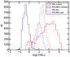 |
Fig. 4 Values of EWα for the models (solid lines) and observations (dashed lines) for star forming regions (red, Q0 / 1 > 0.55) and HOLMES ionized regions (blue, Q0 / 1 < 0.55). |
We plot in Fig. 3 the comparison between the EWα from the observations and those from the computed models. Three color codes are used: the one in the upper panel is associated with the distance to the Kauffman curve Kdist7. In the middle panel f(OB) is used as color code, while in the bottom panel, the color code follows Q0 / 1. The solid line in the plot represents where both values of EWα are equal.
We plot in Fig. 4 the histograms of EWα for the observation and the models, for the regions ionized by HOLMES (in blue) and by OB stars (in red). These histograms actually correspond to the bottom panel of Fig. 3.
To our knowledge, this is the first time the two values of EWα (observed and modeled) are compared for such a set of objects where a detailed determination of the underlying stellar population is available.
We can easily see that there is a clear trend in the variations of the colors in the middle and lower panels, which shows that the ratio Q0 / 1 is a good indicator of the type of stars dominating the ionizing flux (see also Fig. 2 in Sect. 3.4). The color code used for Q0 / 1 shows that OB stars (red/orange) are the coolest in our sample, while HOLMES are the hottest (violet).
In the upper panel of Fig. 3 we explore how the differences between the observed and modeled EWα are related to the Kdist parameter. We can see that most of the regions below the Kauffman curve (Kdist < 0, blue regions), which correspond to classical H iiregions, have observed values of EWα > 10, while most of the regions above the same curve (HOLMES, low-ionization nuclear emission-line region, i.e., LINERS, etc.) have observed values of EWα < 10.
The distribution of the source of the ionizing photons described by f(OB) and Q0 / 1 are clearly bimodal: there is no example of regions ionized by OB stars in a proportion around 50%. This means that we found a clear separation in the models between classical H ii regions and regions ionized by old stars. Figure 3 also shows the contours enclosing the two different populations highlighted in each panels: the models located above and below the Kauffman curve (positive and negative values of Kdist, respectively, top panel) and the regions ionized by OB stars and by HOLMES (value of f(OB) and Q0 / 1, middle and lower panels, respectively). This indicates whether these two populations are distinguishable using the values of EWα.
The EWα is related to the ratio between the number of ionizing photons actually processed by the gas and the number of ionizing stars. Both the gas and the stars are supposed to be included in the observed beam. We can see from Fig. 3 that there is an obvious trend between the observed and modeled EWα. The regions lying on the right side of the y = x line, thus having an observed EWα lower than the modeled value, correspond to regions where fewer photons are ionizing the gas than is expected in a closed geometry model, leading to what is commonly called “leaking”.Stasińska et al. (2001) also proposed the presence of old populations to explain this discrepancy, but we include these old stars in our modeling process. This leaking can be due to matter-bounded regions (in which there is not enough material to be ionized in some directions from the ionizing source point of view) or because of a covering factor of less than one (in some directions there is no gas at all), or even a combination of the two effects. In both cases, some ionizing photons escape the region. In the case of a covering factor that is less than one, the photoionization models correctly predict the line ratios (only the absolute fluxes are overestimated, all in the same proportions) contrary to the case of matter-bounded regions. The presence of strong [O i] and [O ii] emission lines favors the idea of these H ii regions having a covering factor of less than one, then validating the use of the photoionization models.
On the other side of the y = x line (i.e., left), the EWα from the observations is higher than the value from the models. This corresponds to regions where there is more ionized gas than can be ionized by the observed stellar population.It means that we are missing some of the ionizing sources for these regions. It can actually be the effect of photons coming from sources out of the beam, perhaps escaping from the same regions previously described (located on the right side of the line). It would be very interesting to estimate the number of leaking photons in each galaxy and then see if there are enough of them to explain the discrepancies in the EWα determined from observations and models, but this is beyond the scope of this paper.
The difference between the observed and the modeled EWα is clearly related to the proportion of OB stars (top and middle panels of Fig. 3) or the hardness of the ionizing radiation (bottom panel). Most of the star forming regions are located on the right side of the y = x line and correspond to photon leaking. On the other hand, the regions mainly photoionized by HOLMES are only on the left side and correspond to regions ionized by additional sources. The same conclusion can be reached by analyzing Fig. 4 where the observed star forming regions (red dashed line) have a median log(EWα) of ~ 1.3, while the corresponding models have a median log(EWα) of ~ 1.9, leading to a factor of leaking ~ 4 (80% of the photons escape). This median leaking is the same if we use EWβ as all the equivalent widths are shifted by ~−0.5 dex. We note that the distribution of the EWα values for the models of H ii regions is broader than the distribution of the observed values, reflecting the variety of morphologies leading to leaking factors from 1.0 (no leaking) to some tens (see also Papaderos et al. 2013). When considering regions ionized by HOLMES (blue lines in Fig. 4), we see that the discrepancy between the observed and modeled values of EWα goes in the other direction (regions in the left part of the Figs. 3), with log(EWα) median values of ~ 1.0 and ~−0.3 for observation and models, respectively.
Previous studies have analyzed the nature of the LINER-like emission in galaxies (Papaderos et al. 2013; Singh et al. 2013; Sarzi et al. 2010). All of them concluded that the nature of this ionization is most probably due to post-AGBs stars, i.e., HOLMES in our nomenclature. In particular Papaderos et al. (2013) and Gomes et al. (2016) have presented a comparison between the observed Hα fluxes and the predicted ones based on photoionization models whose ionizing source was selected from the analysis of the underlying stellar population for a sample of early-type galaxies. Thus, their analysis is somehow similar to the one presented here. They found that there are two kinds of galaxies on the basis of this comparison: type i, for which the observed and predicted fluxes match very well, in general, and type ii, for which they describe a deficit of observed flux, compatible with a Lyman-continuum leaking, in agreement with the results presented here. We need to recall that the selection procedure adopted has excluded a substantial fraction of the diffuse regions, which are those that dominate the type i ETGs.
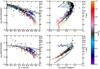 |
Fig. 5 Electron temperature diagnostic line ratios as a function of O/H (left panels) and ([O iii]λ5007 + [O ii]λ3727)/Hβ (right panels) for our models (colored circles). From top to bottom, the diagnostics are [O iii]λ4363/λ5007 and [N ii]λ5755/λ6584. Black diamonds represent the Te-based sample of H ii regions used by Marino et al. (2013). The dashed lines correspond to the grid of models computed by Dopita et al. (2013). The color bar follows Q0 / 1, the softness of the ionizing radiation. |
We must note that state-of-the-art population spectral synthesis models are still plagued by significant degeneracies (e.g., the notorious age–metallicity degeneracy) and uncertainties in the best-fitting star formation history. A tiny variation/uncertainty in the mass fraction of young (< 15−20 Myr) ionizing stars (simple stellar population-SSP models in this study) results in a very significant change in the expected value of Q0, consequently the Balmer recombination line luminosities. On the other hand, the discrepancy between the observed and modeled EWα in the case of HOLMES can just come from an underestimation of the ionizing flux from post-AGBs. This short-lived, highly variable period of the evolution of stars is not very well understood, and its inclusion in SSP models is quite recent, and still presents large uncertainties. Even in the case when we correctly derive the fraction of SSPs comprising post-AGBs, the predicted ionizing photon distribution may still not be totally correct. For all these reasons we prefer not to include the regions ionized by HOLMES in further analysis (see next section), and concentrating on the much better understood regions that are ionized by young stars. In further studies we will try to improve our analysis by (1) excluding or subtracting the possible contribution of a central AGN, if feasible; and (2) updating as much as possible the SSPs and the ionization models adopted for post-AGB stars.
3.6. BPT-population filter
The regions that correspond to star forming regions in the BPT diagram (negative Kdist values) and that are on the left side of the y = x line in the Fig. 3.5 do not lead to trustable models because the ionizing source should be of OB star type, and what is obtained from the SSP decomposition is of HOLMES type. We apply another filter to the ad hoc models to remove objects that have negative Kdist values and that are ionized by old populations. Applying this BPT-population filter to the ad hoc models already filtered by [O ii]/Hβ leads to a set of 2558 models, of which 76% are star forming regions, and 24% are regions ionized by HOLMES and which are over the Kaufmann curve. In the 3MdB database, we set to 1 the value for the com8 field for the models that fit this filter (and 0 otherwise).
The final 2558 models used in the next section fit the [N ii], [O ii], and [O iii] lines with the following mean value and standard deviation: [N ii]/Hβ Model/Obs = 1.05 ± 0.08, [O ii]/Hβ Model/Obs = 0.98 ± 0.13, and [O iii]/Hβ Model/Obs = 1.04 ± 0.14.
In the following sections, the figures show the star forming regions and those ionized by HOLMES, but we select only star forming regions to compute fits to our results, given that we are actually not sure about the pertinence of the HOLMES models (even after applying the filter described above): the missing photons may have a very different distribution, and the O/H abundance have been obtained using the O3N2 ratio, calibrated on H ii regions, not on HOLMES-ionized regions.
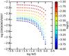 |
Fig. 6 Electron temperature diagnostic line ratios [O iii]λ4363/5007 vs. N/O. The color bar indicates |
4. Results and discussion
In all the following sections, we will present results obtained using the ad hoc Neb models selected after applying the [OII] filter described in Sect. 3.3 and the BPT-population filter described in Sect. 3.6.
4.1. Models nearly compatible with the direct method
In Fig. 5, we show the values of two Te-diagnostic line ratios as a function of the oxygen abundance (left panels) and the ([O ii]λ3727 + [O iii]λ5007)/Hβ line ratio (right panels) for the photoionization models (only the Neb models, colored circles), along with one of the largest and most up-to-date compilations of H ii regionswhere O/H is derived using the direct method (M13) and for a set of observations used by Marino et al. (2013) (black diamonds). The top and bottom panels show the respective [O iii]λ4363/5007 and [N ii]λ5755/6584 diagnostics.
We find a good agreement between the models and the observations in all the panels for metallicities corresponding to 12 + log (O / H) > 8.2. Our star forming region models (orange/red/purple models) fall over the coolest observed regions, pointing to a small underestimation of the electron temperature (but see below). The HOLMES ionizing models (turquoise/blue) are located in the hottest regions. This indicates that the set of models computed for this work, for which the O abundances have been calculated with the O3N2 method, is globally compatible with the determination of O/H using a direct method. The Stel models also decrease in the same regions in these diagrams, leading to the conclusion that this behavior is not due to the way we define O/H. Other previous sets of photoionization models systematically show discrepancies between the values used as input for the O abundances and the values determined from the direct method (e.g., López-Sánchez et al. 2012). This is illustrated with the MAPPINGS models presented in Fig. 5 with a grid that shows the model results obtained from the tables published electronically by Dopita et al. (2013). All these O/H values are systematically larger than those obtained with the direct method (black diamonds), while the results for our models cover the same region and describe the same trend. If we consider only star forming regions, our models are a little bit too cold as they reproduce only half of the observed values of [O iii]λ4363/5007. As far as we know this is the first time that it has been possible to reconcile the predictions by photoionization models with at least a significant amount of direct estimations of the abundance and the line ratios.
In the right panels we can see the differences between the models obtained for this work and the Dopita et al. (2013) models obtained with MAPPINGS. While our models show a very good agreement with the observations, we can see in the upper and middle panels that some of the MAPPINGS models fall in a region where no observations are found (around the data points cloud).
The main differences between the two sets of models seems to be the Te obtained for a given value of O/H, depicted for example by a difference of ≃ 0.5 dex in [O iii]λ4363/5007 at log (O / H) = −3.5, MAPPING models being hotter. This is probably the result of a lower heating or a higher cooling in our models. A higher heating in the Dopita et al. (2013) models can be explained by their use of Starburst99 models from 2005, which provides a harder radiation field than the newest models. In contrast, we use in our models the SED predicted by the POPSTAR models (Mollá et al. 2009).
A higher cooling can be due to our higher values of N/O for a given O/H (see Sect. 4.5), our lower values of for a given O/H (see Sect. 4.6), or because we do not consider the depletion of some elements. To test the effect of N/O and on the electron temperature, we extract a subset of models from 3MdB (Morisset et al. 2015). We use the “HII_CHIm” models (Pérez-Montero 2014) with log (O / H) = −3.5 and an age of the ionizing stellar cluster of 1 Myr, N/O and left free. We show in Fig. 6 effects on the line ratio [O iii]λ4363/5007 of changing N/O (on the x-axis) and (the color code). We can see that a difference in log(N/O) from −0.8 to −1.5 implies a very small difference on the Te-diagnostic line ratio (≃ 0.05 dex). Changing from −2.5 to −3.5 also leads to a very small effect on [O iii]λ4363/5007 (≃ 0.05 dex). To test the effect of the depletion of some elements on the electron temperature we run two models, the first with the abundances from Asplund et al. (2009) as used in our models and the second with a depletion of 1 dex for Si and Mg and of 1.5 dex for Fe. The effect on the line ratio [O iii]λ4363/5007 is an increase of 0.09 dex, not enough to explain the observed difference of ≃ 0.5 dex at log (O / H) ≃ −3.5, but almost enough to increase the ratio to the region where the observations are.
We conclude that the differences observed in Fig. 5 (especially in the upper left panel) between our grid of models and the models from Dopita et al. (2013) are not due to the differences in N/O or the differences in , or whether depletion is used. It may reside in the choice of the ionizing SED, if not from the code used. In summary, our photionization models are almost compatible with the electron temperature derived from the direct method at a given O/H, and are the first ones in the literature to our knowledge. Our electron temperature is a little bit cool, perhaps pointing to a small lack of depletion of some elements or the presence of some light extra heating process or the presence of a process favoring the emission of high temperature lines (temperature fluctuations à la Peimbert 1967, κ distribution à la Nicholls et al. 2012). Indeed, the differences in the selected ionizing source could explain and solve the long-standing incompatibility between the direct method and photoionization models, and we present here a set of models approaching the observational reality.
4.2. BPT diagram
Figure 7 shows our photoionization models in the classical BPT diagram (Baldwin et al. 1981), log ([O iii]/Hβ) versus log ([N ii]/Hα). The curves derived by Kauffmann et al. (2003), Kewley & Dopita (2002) and Stasińska et al. (2006) have been included in the plots for reference. These curves are often used to distinguish between star forming regions (below the envelope empirically defined by Kauffmann et al. 2003) and AGNs (above the envelope defined by Kewley & Dopita 2002). The color bars located on the right side run from low to high values of the O abundance, the N/O ratio, the Hα equivalent widths (determined from observations and from models), the ionization parameter , and the fraction of OB stars f(OB) (from upper left to lower right panels, respectively). We plot here only the results concerning the models where the O/H abundance is determined from the O3N2 relation from M13 (Neb models, see Sect. 3.1).
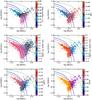 |
Fig. 7 Classical BPT diagrams of the model results. For each panel, the color code is changed according to the description on the right of the corresponding color bar. The upper panels show distributions of the models, with colors related to the chemical abundances: O/H on the left and N/O on the right. The middle panels show the distribution of the Hα equivalent width determined from the observations and from the models in the left and right panels, respectively. The lower panels show the distribution of the mean ionization parameter |
We can see from the middle panels that there is a general trend of the models with lower EWα and lower f(OB) located above the Kauffmann et al. (2003) curve, although there are also models with low EWα and low f(OB) below this curve. We can also see that there are no photoionization models with high EWα and f(OB) above the Kewley & Dopita (2002) curve. Our models reproduce the observational results obtained by Sánchez et al. (2015): below the curve the models with higher O abundance and lower U are located in the lower right region, whereas those with a low O abundance and high U are located in the upper left corner (Evans & Dopita 1985; Veilleux & Osterbrock 1987; López-Sánchez et al. 2012). We note that the middle left plot uses only observed data and then shows a greater number of points. The color separation in the BPT diagram is clearer when using the observed EWα (left panel), while the mixing of the colors is more important for the EWα from the models (right panel). This is consistent with the results from Fig. 3 described in Sect. 3.5: the observed EWα may appear to be a very good diagnostic for the ionizing population (and for determining the kind of nebular region observed), but when using the EWα from the models, the situation is much less obvious.
In the lower left panel of Fig. 7 we use as the color code. It shows a clear gradient of decreasing in the decreasing [O iii]/Hβ-increasing [N ii]/Hα direction.In the lower right panel of Fig. 7 we use f(OB) as the color code. As in Fig. 3, the two extreme values of f(OB) dominate the distribution and are not very well separated. We can also see some regions where HOLMES dominates the ionizing SED well inside the star forming region, while almost no OB stars dominated regions enter the part of the BPT diagram between the Kauffman and the Kewley curves, and not at all above the Kewley curve, in agreement with the definition of these demarcation line.
Figure 8 shows the comparison between different BPT-type diagrams taken from Baldwin et al. (1981), Veilleux & Osterbrock (1987): [O iii]/Hβ versus [N ii]/Hα, [O iii]/Hβ versus [O ii]/[O iii], [N ii]/Hβ versus [O ii]/[O iii], and [O i]/Hα versus [O ii]/[O iii]. In these plots, we use the Q0 / 1 ratio as the color code, tracing the softness of the ionizing flux.
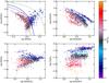 |
Fig. 8 BPT diagrams inspired by Baldwin et al. (1981). The color code represents the hardness of the radiation Q0 / 1. The solid blue line is from Kauffmann et al. (2003), the green dashed line is from Kewley et al. (2001), and the dotted black line is from Stasińska et al. (2006). |
The [O iii]/Hβ versus [O ii]/[O iii] and [O i]/Hα versus [O ii]/[O iii] ratios (upper right and lower right panels, respectively) do not depend on the N/O abundance ratio. Both plots exhibit a clear separation between the regions ionized by OB stars (Q0 / 1 > 0.55) and those ionized by HOLMES otherwise, but we note that in the [O iii]/Hβ versus [O ii]/[O iii] plot, some regions ionized by HOLMES are mixed with the OB star ionized regions whereas the separation in the [O i]/Hα versus [O ii]/[O iii]plot is clearer (in agreement with the results pointed out by Baldwin et al. 1981). It should be noted that the values of [O i]/Hα used here are pure predictions from the models, and do not necessarily reproduce the observations.
4.3. WHAN diagram
Figure 9 shows the WHAN diagram for our models. This diagram is based on Hα and [N ii] lines and was proposed by Cid Fernandes et al. (2010) to determine the ionizing population. In the left panel we show the EWα from the models and in the right panel the values derived from the observations.
The general trend is that the regions ionized by OB stars have higher EWα than the regions ionized by HOLMES (the EWα from the models cover a wider range of values than the EWα derived from the observations).
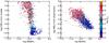 |
Fig. 9 WHAN diagrams: values of EWα from the models (left panel) and from the observations (right panel) as a function of [N ii]/Hα. The color code represents the proportion of OB stars. |
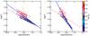 |
Fig. 10
|
The separation between the regions ionized by OB stars and those ionized by HOLMES is very clear when using the EWα from the models, whereas the different type of ionized regions are more mixed in the other panel. Another interesting result from this figure is that there is no correlation between the EWα from the models and the [N ii]/Hα ratios, but there is a clear trend between the EWα computed from the observations and the [N ii]/Hα ratios. This indicates that if we only know the [N ii]/Hα ratio we cannot distinguish between regions ionized by OB stars or HOLMES. Thus, the knowledge of the properties of the underlying stellar population is a fundamental tool to distinguish between the two types of regions. This was already discussed by Sanchez et al. (2014). Another interesting result is that while a limit of EWαmod> 3 Å to segregate classical H ii regions from HOLMES is clearly predicted by the models, in practice an empirical cut of EWα> 6 Å or the demarcation line  (3)seems to separate both ionizing regions better.
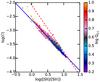 |
Fig. 11
|
4.4.  versus O II/O III and S II/S III
The [O ii]/[O iii] and [S ii]/[S iii] line ratios have frequently been used as tracers of the ionization strength (Diaz 2001; Kewley & Dopita 2002) based on empirical correlations between these line ratios and this parameter (Dors & Copetti 2003). However, as we have seen along this article, previous results are sometimes based on photoinization models whose ionization source was not selected to match any observed constraint. Therefore, it is important to revise the trends between those parameters based on our new set of models. In Figs. 10 and 11, we explore the relations between and the [O ii]/[O iii] and [S ii]/[S iii] line ratio, respectively.
In Fig. 10 we show the first of these relations for each of the geometries considered in our models: thin shell and empty sphere (left and right panel, respectively). We overplot the relation determined by Díaz et al. (2000, hereafter D00). This relation does not match the results of our models, especially the values corresponding to star forming regions (Q0 / 1 > 0.55, gray/red points). In the case of thin shell geometry (left panel), there is an underestimation of by ~0.25 dex with a scatter of approximately the same amount. In the case of a geometrically thick region (right panel), the slope of the D00 relation is not recovered. Our results indicate that there is a steeper relation, although the average value is similar to that predicted by D00. Our fits limited to the regions where Q0 / 1 > 0.55 (star forming regions) leads to  (4)with a standard deviation of 0.14 and to
  (5)with a standard deviation of 0.22, for the left panel (thin shells) and right panel (filled spheres), respectively.
In Fig. 11 we do not split the two geometries in different plots, as the results are very similar for each of them. A tighter relation is derived in comparison with the one derived for [O ii]/[O iii]. We overplot the relation determined by Diaz et al. (1991), showing a different slope but similar values at low ionization. The changes in the atomic data (especially for [S ii]) since 1991 may explain the differences. The following linear fit, limited to the regions where Q0 / 1 > 0.55 (star forming regions), is obtained:  (6)with a standard deviation of 0.06.
4.5. N/O versus O/H
The nucleosynthesis paths for nitrogen and oxygen are different. The origin of nitrogen is both primary, produced from the initial content of hydrogen, and secondary, produced from the initial content of carbon and oxygen created by previous stellar generations (e.g., Matteucci 1986). Therefore, the N/H and O/H abundance ratios are not supposed to evolve in lockstep. The N/O versus O/H relation derived from observations is mainly horizontal for log(O/H) < –4.1 where the nitrogen is of primary production, and almost linear above this, where the secondary production of nitrogen take place (see, e.g., Vila Costas & Edmunds 1993; Thurston et al. 1996; Chiappini et al. 2003; Liang et al. 2006; Mollá et al. 2006, and references therein). The regions we use in this work are all above this limit and only allow us to probe the linear part of the relation.
Figure 12 shows the relation between the abundance ratio N/O and the oxygen abundance O/H. The left and right panels use different color codes: stellar population as depicted by the softness parameter Q0 / 1 and respectively. We note that the N/O abundance ratio is one of the main results, with , of the fitting process we applied, see Sect. 3.1.
The difference between the regions ionized by OB stars and by HOLMES is shown in the left panel: at a given metallicity, the N/O ratio is lower in the second group (Q0 / 1 < 0.55, blue points) than in the classical star forming regions (Q0 / 1 > 0.55). This is also the case even if we define the nebular metallicity from the stellar content (Stel models, see Sect. 4.8). These differences in the N/O determinations may be an indication that the amount of nitrogen of the regions ionized by HOLMES is systematically lower than in the star forming regions.
If we concentrate on the star forming regions alone, we can determine a linear fit to the relation between N/O and O/H  (7)with a standard deviation of 0.13.
This fit is valid only on the O/H range available with the data used here, namely between 8.1 < 12 + log (O / H) < 8.8. There a clear color gradient following in the right panel, pointing to a second-order effect of the gas ionization stage on the relation.
We compare this fit to the ones determined by Pilyugin et al. (2012, light green dashed line) and by Dopita et al. (2013, red dotted line). There is a good agreement with the first, and a clear offset with respect to the second. This result is expected since Pilyugin et al. (2012) adopts oxygen abundances derived using a direct method, while Dopita et al. (2013) uses a particular set of photoioniziation models that overestimate the abundances. Again, the result confirms our previous claim that our photoinization models are compatible with direct method estimations, contrary to some previous results.
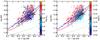 |
Fig. 12 N/O vs. O/H. Left panel: the color codes the hardness of the ionizing radiation Q0 / 1. Right panel: the color codes the value of |
4.6. versus O/H
We plot in Fig. 13 the position of the models in the versus 12 + log(O/H) diagram. We also added the empirical relations from Dopita & Evans (1986), Dopita et al. (2006), and Pérez-Montero (2014). We can easily see that the values of we determined are lower by around 0.7 dex than the values obtained from these relations or that our oxygen abundance is between 0.4 and 0.7 dex lower, depending on the relation we consider. This apparent discrepancy is principally due to the way we determined the oxygen abundance (using O3N2 from M13); using the abundance estimator from e.g., Kewley & Dopita (2002) would lead to higher values for O/H and could reconcile the values we obtained with the different relations shown here (see also the discussion of the results obtained with the Stel models in Sect. 4.8).
The effect of the ionizing stellar population (used for the color code) is also very clear. The values for the regions ionized by HOLMES are 0.5 dex lower than for the classical H ii regions (ionized by OB stars).
Our fits to the models corresponding to star forming regions (Q0 / 1 > 0.55) are  (8)and
  (9)with a standard deviation of 0.20 for the left panel (thin shell) and 0.36 for the right panel (filled sphere), respectively. We note the very high uncertainties and dispersion in the case of filled sphere models.
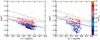 |
Fig. 13
|
4.7. Variation of the η parameter with the ionizing SED
Following Vilchez & Pagel (1988), we plot in Fig. 14 the values of η = (O+/O++)/(S+/S++) versus S+/S++ and η′ = ([O ii]λ3727+/[O iii]λ5007+)/([S ii]λ6720+/[S iii]λ9067+) versus [S ii]λ6720+/[S iii]λ9067+. We show that these values of η and η′ depend on the softness of the ionizing SED, represented here by Q0 / 1 as color code, as already pointed out by Vilchez & Pagel (1988). We also see here that the η′ depends strongly on the geometry as well, the left panel being the thin models (fr = 3.0) and right panels the filled sphere models (fr = 0.03). Given the scatter observed in each panel and the relatively high difference between the two geometries, the relation between the values of η and the softness of the ionizing radiation Q0 / 1 is far from being established.
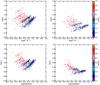 |
Fig. 14 Relation between η = (O+/O++)/(S+/S++) and S+/S++ (upper panels) and between η′ = ([O ii]λ3727+/[O iii]λ5007+)/ ([S ii]λ6720+/[S iii]λ9067+) and [S ii]λ6720+/[S iii]λ9067+ (lower panels). Left panel: thin shell models (fr = 3.0), right panel: filled sphere models (fr = 0.03). The color code follows the Q0 / 1 ratio (see text). |
4.8. Effect of the nebular abundance determination on the results
We redraw all the figures presented in the previous sections, but now using the models obtained with the Stel determination of the nebular O/H (see Sect. 3.1). The corresponding figures are available in Appendix A.The main differences between the two sets of models are obviously seen in plots directly involving the nebular metallicity, for example in the upper left panel of Figs. 7 and A.1 (Neb and Stel models, respectively) where the color distribution is strongly affected. We note that the position of the models in all the BPT diagrams are the same as each model is reproducing the [N ii]/Hα, [O ii]/Hβ, and [O iii]/Hβ line ratio, however its nebular metallicity is obtained.
The results related to the relation between and [O ii]/[O iii] shown in Figs. 10/A.2 are slightly affected, but the main conclusion remains unchanged: the relation from Díaz et al. (2000) is not recovered. When using [S ii]/[S iii] as in Figs. 11, there is a perfect match between the two sets of models. This leads to the conclusion that the results obtained here, in particular the fit from Eq. (6) (but also Eqs. (4) and (5)), are very robust.
The more important differences are obtained for Figs. 12 and A.3 and Figs. 13 and A.4 showing the relations between and N/O versus O/H, respectively. Clear relations are not obtained at all when the nebular metallicity is derived from the stellar content (Stel models). Nevertheless, these two relations exist and have been observed using other methods. The lack of relation between and N/O versus O/H when using the Stel models indicates that (1) the Stel models are not correct regarding the nebular metallicity; and (2) that these relations obtained with the Neb models may be dependent on the way the nebular metallicity is obtained.
5. Conclusions
We present in this paper a set of photoionization models based on the CALIFA H ii regions catalog. Each model uses as ionizing SED the combination of POPSTAR stellar population models (Mollá et al. 2009) based on the analysis of the continuum spectra performed by the FIT3D program (Sánchez et al. 2011) for the corresponding region. Each model corresponds to an interpolation in the versus N/O parameter space to fit the observation of the [N ii]/Hα and [O iii]/Hβ line ratios of an individual H ii region. Two different morphologies (filled or empty spheres) as well as two different ways to derive O/H (from O3N2 and from the stellar population) are explored. The fact that O/H is determined by the strong line method leads to qualifying these models as “hybrid”. We finally filter the models by selecting only the ones that also fit of the [O ii]/Hα line ratio and excluding the ones that correspond to the HOLMES ionizing spectrum and fall in the star forming region of the BPT diagram. We obtain a set of 2558 models, each one fitting simultaneously the tree line ratios of a given H ii region. This incomparable database allows us to explore relations between parameters, with the possibility of taking into account the effect of the way the nebular metallicity is defined or the morphology of the region.
The ionizing stellar population can be divided into two groups: classical OB stars ionizing star forming regions, and HOLMES resulting from the evolution of old starbursts. Three quarters of the models correspond to star forming regions. We find that the first regions show a difference in the Hα equivalent width between models and observations that can be interpreted as the result of a median leaking of 80% of the photons. On the contrary, for the HOLMES ionized regions we found that the models predict higher values for EWα than actually observed. This can be understood as missing ionizing photons compared to what would be needed to produce the HI recombination lines.
We show that our models are mainly compatible with the electron temperature derived from observations for a given value of O/H, which was not the case for previously published grids of models (e.g., Dopita et al. 2013). We attribute the better match of our models to the use of a detailed ionizing SED obtained from the stellar underlying population for each region.
We derive new relations between versus [O ii]/[O iii] and [S ii]/[S iii], showing that the first strongly depends on the morphology of the nebula, while the second one is a very robust result (which does not depend on the way the nebular abundance is determined).
The relation between N/O and O/H we derive is compatible with Pilyugin et al. (2012, using a method based on observations) and not with Dopita et al. (2013, based on photoionization models). The relation between and O/H is different from the previous determinations, leading for lower values at a given metallicity. We also conclude that η′ is not a good indicator of the softness of the radiation field, as it also strongly depends on the morphology of the region.
All the figures presented in this paper can easily be generated by anyone given that the data are available from 3MdB and that the python codes used to make the models and the figures are available from the 3MdB web page8.
In the following we use [N ii], [O i], [O ii], [O iii], [S ii], and [S iii] for the [N ii]λ6584 Å, [O i]λ6300 Å, [O ii]λ3726+29 Å, [O iii]λ5007 Å, [S ii]λ6716+31 Å, and [S iii]λ6312 Å lines, respectively.
The ionization parameter is defined as U(r) = Q(H0) / 4.π.r2.NH.c, where Q(H0) is the number of ionizing photons emitted by the source per unit of time, r is the distance between the source and the nebula, NH is the hydrogen density, and c is the speed of light. We use the mean value of U on the volume of the nebula weighted by the electron density, and name its logarithmic value.
HOLMES stands for HOt Low Mass Evolved Stars, see, e.g., Flores-Fajardo et al. (2011).
The Kdist parameter is defined by the minimum value of the distance D between a given point and the Kauffmann et al. (2003) curve, being negative for points below the curve and positive otherwise. The distance between 2 points in the BPT diagram is defined by  .
.
Acknowledgments
C.M. took advantage of the useful discussions with G. Hägele and his co-workers while a guest at La Plata University.
We thank the anonymous referee for the careful review of the paper and the valuable comments.
We want to thank Yago Ascasibar and Polychronis Papaderos, the internal CALIFA referee for this paper, for their useful comments.
Part of the results presented here have been obtained using computers from the CONACyT project CB2010/153985 and the UNAM-PAPIIT project 107215. The computers “Tychos” (Posgrado en Astrofísica-UNAM, Instituto de Astronomia-UNAM and PNPC-CONACyT) have been used for this research.
G.D.I. gratefully acknowledges support from the Mexican CONACYT grant CB-2014-241732.
S.F.S. thanks the CONACYT-125180 and DGAPA-IA100815 projects for providing support during this study.
Support for L.G. is provided by the Ministry of Economy, Development, and Tourism’s Millennium Science Initiative through grant IC120009, awarded to The Millennium Institute of Astrophysics, MAS. L.G. acknowledges support by CONICYT through FONDECYT grant 3140566.
This study uses data provided by the Calar Alto Legacy Integral Field Area (CALIFA) survey (http://califa.caha.es/). CALIFA is the first legacy survey performed at Calar Alto. The CALIFA collaboration would like to thank the IAA-CSIC and MPIA-MPG as major partners of the observatory, and CAHA itself, for the unique access to telescope time and support in manpower and infrastructures. The CALIFA collaboration also thanks the CAHA staff for the dedication to this project.
Based on observations collected at the Centro Astronómico Hispano Alemán (CAHA) at Calar Alto, operated jointly by the Max-Planck-Institut für Astronomie and the Instituto de Astrofísica de Andalucia (CSIC).
References
- Anderson, L. D. 2014, in Am. Astron. Soc. Meet. Abstr., 223, 312.01 [Google Scholar]
- Asplund, M., Grevesse, N., Sauval, A. J., & Scott, P. 2009, ARA&A, 47, 481 [NASA ADS] [CrossRef] [Google Scholar]
- Baldwin, J. A., Phillips, M. M., & Terlevich, R. 1981, PASP, 93, 5 [NASA ADS] [CrossRef] [EDP Sciences] [Google Scholar]
- Binette, L., Magris, C. G., Stasińska, G., & Bruzual, A. G. 1994, A&A, 292, 13 [NASA ADS] [Google Scholar]
- Binette, L., Flores-Fajardo, N., Raga, A. C., Drissen, L., & Morisset, C. 2009, ApJ, 695, 552 [NASA ADS] [CrossRef] [Google Scholar]
- Cairós, L. M., Caon, N., García Lorenzo, B., et al. 2012, A&A, 547, A24 [NASA ADS] [CrossRef] [EDP Sciences] [Google Scholar]
- Calzetti, D. 2001, PASP, 113, 1449 [NASA ADS] [CrossRef] [Google Scholar]
- Chabrier, G. 2003, PASP, 115, 763 [NASA ADS] [CrossRef] [Google Scholar]
- Chiappini, C., Romano, D., & Matteucci, F. 2003, MNRAS, 339, 63 [NASA ADS] [CrossRef] [Google Scholar]
- Cid Fernandes, R., Stasińska, G., Schlickmann, M. S., et al. 2010, MNRAS, 403, 1036 [NASA ADS] [CrossRef] [Google Scholar]
- Cid Fernandes, R., Pérez, E., García Benito, R., et al. 2013, A&A, 557, A86 [NASA ADS] [CrossRef] [EDP Sciences] [Google Scholar]
- Cid Fernandes, R., González Delgado, R. M., García Benito, R., et al. 2014, A&A, 561, A130 [NASA ADS] [CrossRef] [EDP Sciences] [Google Scholar]
- Diaz, M. 2001, in Spectroscopic Challenges of Photoionized Plasmas, eds. G. Ferland, & D. W. Savin, ASP Conf. Ser., 247, 227 [Google Scholar]
- Diaz, A. I., Terlevich, E., Vilchez, J. M., Pagel, B. E. J., & Edmunds, M. G. 1991, MNRAS, 253, 245 [NASA ADS] [CrossRef] [Google Scholar]
- Díaz, A. I., Castellanos, M., Terlevich, E., & Luisa García-Vargas, M. 2000, MNRAS, 318, 462 [NASA ADS] [CrossRef] [Google Scholar]
- Dopita, M. A., & Evans, I. N. 1986, ApJ, 307, 431 [NASA ADS] [CrossRef] [Google Scholar]
- Dopita, M. A., Kewley, L. J., Heisler, C. A., & Sutherland, R. S. 2000, ApJ, 542, 224 [NASA ADS] [CrossRef] [Google Scholar]
- Dopita, M. A., Fischera, J., Sutherland, R. S., et al. 2006, ApJ, 647, 244 [NASA ADS] [CrossRef] [Google Scholar]
- Dopita, M. A., Sutherland, R. S., Nicholls, D. C., Kewley, L. J., & Vogt, F. P. A. 2013, ApJS, 208, 10 [NASA ADS] [CrossRef] [Google Scholar]
- Dors, Jr., O. L., & Copetti, M. V. F. 2003, A&A, 404, 969 [NASA ADS] [CrossRef] [EDP Sciences] [Google Scholar]
- Dottori, H. A. 1987, Rev. Mexicana Astron. Astrofis., 14, 463 [NASA ADS] [Google Scholar]
- Dottori, H. A., & Copetti, M. V. F. 1989, Rev. Mexicana Astron. Astrofis., 18, 115 [NASA ADS] [Google Scholar]
- Draine, B. T. 2011, ApJ, 732, 100 [NASA ADS] [CrossRef] [Google Scholar]
- Evans, I. N., & Dopita, M. A. 1985, ApJS, 58, 125 [NASA ADS] [CrossRef] [Google Scholar]
- Falcón-Barroso, J., Sánchez-Blázquez, P., Vazdekis, A., et al. 2011, A&A, 532, A95 [NASA ADS] [CrossRef] [EDP Sciences] [Google Scholar]
- Ferland, G. J., Porter, R. L., van Hoof, P. A. M., et al. 2013, Rev. Mexicana Astron. Astrofis., 49, 137 [Google Scholar]
- Fitzpatrick, E. L. 1999, PASP, 111, 63 [NASA ADS] [CrossRef] [Google Scholar]
- Flores-Fajardo, N., Morisset, C., & Binette, L. 2009, Rev. Mex. Astron. Astrofis., 45, 261 [NASA ADS] [Google Scholar]
- Flores-Fajardo, N., Morisset, C., Stasińska, G., & Binette, L. 2011, MNRAS, 415, 2182 [NASA ADS] [CrossRef] [Google Scholar]
- García-Benito, R., Pérez, E., Díaz, Á. I., Maíz Apellániz, J., & Cerviño, M. 2011, AJ, 141, 126 [NASA ADS] [CrossRef] [Google Scholar]
- García-Benito, R., Zibetti, S., Sánchez, S. F., et al. 2015, A&A, 576, A135 [NASA ADS] [CrossRef] [EDP Sciences] [Google Scholar]
- Gomes, J. M., Papaderos, P., Kehrig, C., et al. 2016, A&A, 588, A68 [NASA ADS] [CrossRef] [EDP Sciences] [Google Scholar]
- GonzálezDelgado, R. M., & Perez, E. 1997, ApJS, 108, 199 [NASA ADS] [CrossRef] [Google Scholar]
- González Delgado, R. M., Pérez, E., Cid Fernandes, R., et al. 2014, A&A, 562, A47 [NASA ADS] [CrossRef] [EDP Sciences] [Google Scholar]
- Hodge, P. W., & Kennicutt, Jr., R. C. 1983, ApJ, 267, 563 [NASA ADS] [CrossRef] [Google Scholar]
- Husemann, B., Jahnke, K., Sánchez, S. F., et al. 2013, A&A, 549, A87 [NASA ADS] [CrossRef] [EDP Sciences] [Google Scholar]
- Kauffmann, G., Heckman, T. M., Tremonti, C., et al. 2003, MNRAS, 346, 1055 [Google Scholar]
- Kehrig, C., Vílchez, J. M., Sánchez, S. F., et al. 2008, A&A, 477, 813 [NASA ADS] [CrossRef] [EDP Sciences] [Google Scholar]
- Kehrig, C., Monreal-Ibero, A., Papaderos, P., et al. 2012, A&A, 540, A11 [NASA ADS] [CrossRef] [EDP Sciences] [Google Scholar]
- Kelz, A., Verheijen, M. A. W., Roth, M. M., et al. 2006, PASP, 118, 129 [NASA ADS] [CrossRef] [Google Scholar]
- Kewley, L. J., & Dopita, M. A. 2002, ApJS, 142, 35 [NASA ADS] [CrossRef] [Google Scholar]
- Kewley, L. J., Dopita, M. A., Sutherland, R. S., Heisler, C. A., & Trevena, J. 2001, ApJ, 556, 121 [Google Scholar]
- Knapen, J. H. 1998, MNRAS, 297, 255 [NASA ADS] [CrossRef] [Google Scholar]
- Liang, Y. C., Yin, S. Y., Hammer, F., et al. 2006, ApJ, 652, 257 [NASA ADS] [CrossRef] [Google Scholar]
- Lopez, L. A., Krumholz, M. R., Bolatto, A. D., Prochaska, J. X., & Ramirez-Ruiz, E. 2011, ApJ, 731, 91 [NASA ADS] [CrossRef] [Google Scholar]
- López-Sánchez, A. R., & Esteban, C. 2009, A&A, 508, 615 [NASA ADS] [CrossRef] [EDP Sciences] [Google Scholar]
- López-Sánchez, Á. R., Dopita, M. A., Kewley, L. J., et al. 2012, MNRAS, 426, 2630 [NASA ADS] [CrossRef] [Google Scholar]
- Marino, R. A., Rosales-Ortega, F. F., Sánchez, S. F., et al. 2013, A&A, 559, A114 [NASA ADS] [CrossRef] [EDP Sciences] [Google Scholar]
- Marino, R. A., Gil de Paz, A., Sánchez, S. F., et al. 2016, A&A, 585, A47 [NASA ADS] [CrossRef] [EDP Sciences] [Google Scholar]
- Martins, L. P., González Delgado, R. M., Leitherer, C., Cerviño, M., & Hauschildt, P. 2005, MNRAS, 358, 49 [NASA ADS] [CrossRef] [Google Scholar]
- Mast, D., Rosales-Ortega, F. F., Sánchez, S. F., et al. 2014, A&A, 561, A129 [NASA ADS] [CrossRef] [EDP Sciences] [Google Scholar]
- Matteucci, F. 1986, MNRAS, 221, 911 [NASA ADS] [Google Scholar]
- Mollá, M., Vílchez, J. M., Gavilán, M., & Díaz, A. I. 2006, MNRAS, 372, 1069 [NASA ADS] [CrossRef] [Google Scholar]
- Mollá, M., García-Vargas, M. L., & Bressan, A. 2009, MNRAS, 398, 451 [NASA ADS] [CrossRef] [Google Scholar]
- Morisset, C. 2013, pyCloudy: Tools to manage astronomical Cloudy photoionization code [Google Scholar]
- Morisset, C. 2014, in Asymmetrical Planetary Nebulae VI conference, Proc. Conf. held 4−8 November, 2013, eds C. Morisset, G. Delgado-Inglada, & S. Torres-Peimbert [Google Scholar]
- Morisset, C., & Georgiev, L. 2009, A&A, 507, 1517 [NASA ADS] [CrossRef] [EDP Sciences] [Google Scholar]
- Morisset, C., Delgado-Inglada, G., & Flores-Fajardo, N. 2015, Rev. Mexicana Astron. Astrofis., 51, 103 [NASA ADS] [Google Scholar]
- Nicholls, D. C., Dopita, M. A., & Sutherland, R. S. 2012, ApJ, 752, 148 [NASA ADS] [CrossRef] [Google Scholar]
- Oey, M. S., Parker, J. S., Mikles, V. J., & Zhang, X. 2003, AJ, 126, 2317 [NASA ADS] [CrossRef] [Google Scholar]
- Osterbrock, D. E. 1989, Astrophysics of gaseous nebulae and active galactic nuclei (University Science Books) [Google Scholar]
- Papaderos, P., Gomes, J. M., Vílchez, J. M., et al. 2013, A&A, 555, L1 [NASA ADS] [CrossRef] [EDP Sciences] [Google Scholar]
- Peimbert, M. 1967, ApJ, 150, 825 [NASA ADS] [CrossRef] [Google Scholar]
- Pérez, E., Cid Fernandes, R., González Delgado, R. M., et al. 2013, ApJ, 764, L1 [NASA ADS] [CrossRef] [Google Scholar]
- Pérez-Montero, E. 2014, MNRAS, 441, 2663 [NASA ADS] [CrossRef] [Google Scholar]
- Pérez-Montero, E., García-Benito, R., Hägele, G. F., & Díaz, Á. I. 2010, MNRAS, 404, 2037 [NASA ADS] [Google Scholar]
- Pilyugin, L. S., Vílchez, J. M., Mattsson, L., & Thuan, T. X. 2012, MNRAS, 421, 1624 [NASA ADS] [CrossRef] [Google Scholar]
- Rémy-Ruyer, A., Madden, S. C., Galliano, F., et al. 2014, A&A, 563, A31 [NASA ADS] [CrossRef] [EDP Sciences] [Google Scholar]
- Rosales-Ortega, F. F., Kennicutt, R. C., Sánchez, S. F., et al. 2010, MNRAS, 405, 735 [NASA ADS] [Google Scholar]
- Rosales-Ortega, F. F., Sánchez, S. F., Iglesias-Páramo, J., et al. 2012, ApJ, 756, L31 [NASA ADS] [CrossRef] [Google Scholar]
- Roth, M. M., Kelz, A., Fechner, T., et al. 2005, PASP, 117, 620 [NASA ADS] [CrossRef] [Google Scholar]
- Salpeter, E. E. 1955, ApJ, 121, 161 [Google Scholar]
- Sánchez, S. F., García-Lorenzo, B., Jahnke, K., et al. 2006, New Astron. Rev, 49, 501 [Google Scholar]
- Sánchez, S. F., Rosales-Ortega, F. F., Kennicutt, R. C., et al. 2011, MNRAS, 410, 313 [NASA ADS] [CrossRef] [Google Scholar]
- Sánchez, S. F., Kennicutt, R. C., Gil de Paz, A., et al. 2012a, A&A, 538, A8 [NASA ADS] [CrossRef] [EDP Sciences] [Google Scholar]
- Sánchez, S. F., Rosales-Ortega, F. F., Marino, R. A., et al. 2012b, A&A, 546, A2 [NASA ADS] [CrossRef] [EDP Sciences] [Google Scholar]
- Sánchez, S. F., Rosales-Ortega, F. F., Jungwiert, B., et al. 2013, A&A, 554, A58 [NASA ADS] [CrossRef] [EDP Sciences] [Google Scholar]
- Sánchez, S. F., Rosales-Ortega, F. F., Iglesias-Páramo, J., et al. 2014, A&A, 563, A49 [NASA ADS] [CrossRef] [EDP Sciences] [Google Scholar]
- Sánchez, S. F., Pérez, E., Rosales-Ortega, F. F., et al. 2015, A&A, 574, A47 [NASA ADS] [CrossRef] [EDP Sciences] [Google Scholar]
- Sánchez, S. F., García-Benito, R., Zibetti, S., et al. 2016a, A&A, 594, A36 [NASA ADS] [CrossRef] [EDP Sciences] [Google Scholar]
- Sánchez, S. F., Pérez, E., Sánchez-Blázquez, P., et al. 2016b, Rev. Mexicana Astron. Astrofis., 52, 21 [Google Scholar]
- Sánchez-Blázquez, P., Peletier, R. F., Jiménez-Vicente, J., et al. 2006, MNRAS, 371, 703 [NASA ADS] [CrossRef] [Google Scholar]
- Sánchez-Menguiano, L., Sánchez, S. F., Pérez, I., et al. 2016, A&A, 587, A70 [NASA ADS] [CrossRef] [EDP Sciences] [Google Scholar]
- Sarzi, M., Shields, J. C., Schawinski, K., et al. 2010, MNRAS, 402, 2187 [NASA ADS] [CrossRef] [Google Scholar]
- Singh, R., van de Ven, G., Jahnke, K., et al. 2013, A&A, 558, A43 [NASA ADS] [CrossRef] [EDP Sciences] [Google Scholar]
- Stasińska, G., Schaerer, D., & Leitherer, C. 2001, A&A, 370, 1 [Google Scholar]
- Stasińska, G., Cid Fernandes, R., Mateus, A., Sodré, L., & Asari, N. V. 2006, MNRAS, 371, 972 [NASA ADS] [CrossRef] [Google Scholar]
- Stasińska, G., Vale Asari, N., Cid Fernandes, R., et al. 2008, MNRAS, 391, L29 [NASA ADS] [Google Scholar]
- Stasińska, G., Izotov, Y., Morisset, C., & Guseva, N. 2015, A&A, 576, A83 [NASA ADS] [CrossRef] [EDP Sciences] [Google Scholar]
- Thurston, T. R., Edmunds, M. G., & Henry, R. B. C. 1996, MNRAS, 283, 990 [NASA ADS] [CrossRef] [Google Scholar]
- Vazdekis, A., Sánchez-Blázquez, P., Falcón-Barroso, J., et al. 2010, MNRAS, 404, 1639 [NASA ADS] [Google Scholar]
- Veilleux, S., & Osterbrock, D. E. 1987, ApJS, 63, 295 [NASA ADS] [CrossRef] [Google Scholar]
- Vila Costas, M. B., & Edmunds, M. G. 1993, MNRAS, 265, 199 [NASA ADS] [CrossRef] [Google Scholar]
- Vilchez, J. M., & Pagel, B. E. J. 1988, MNRAS, 231, 257 [NASA ADS] [CrossRef] [Google Scholar]
- Walcher, C. J., Wisotzki, L., Bekeraité, S., et al. 2014, A&A, 569, A1 [NASA ADS] [CrossRef] [EDP Sciences] [Google Scholar]
- York, D. G., Adelman, J., Anderson, Jr., J. E., et al. 2000, AJ, 120, 1579 [Google Scholar]
Appendix A: Results obtained from the Stel models
In this Appendix, we present the same figures shown in the paper, but obtained with the Stel abundance determination, instead of Neb (See Sects. 3.1 and 4.8). We only show the figures significantly different from the Neb case.
All Figures
|
Fig. 1 Modeled BPT diagram [O iii]/Hβ vs. [N ii]/Hα used to interpolate the values of |
| In the text | |
|
Fig. 2 Values of Q0 / 1 = Q(H0)/Q(He0) for the OB and HOLMES dominated spectra. |
| In the text | |
|
Fig. 3 Comparison between the EWα from the models and from the observations. Colors represent Kdist, the distance to the Kauffmann et al. (2003) curve (upper panel), the OB stars proportion f(OB) (middle panel), and the ratio Q0 / 1 = Q(He0)/Q(H0) (lower panel). The solid blue line follows y = x. In the upper panel, the solid black curves enclose half of the models that are below the Kauffman curve (negative Kdist), while the dashed black curve encloses half of the models above the same curve (positive Kdist). In the middle panel, the solid black contour encloses half of the models ionized by OB stars (f(OB) > 0.5), while the dashed black contour encloses half of the models ionized by HOLMES (f(OB) < 0.5). In the lower panel, the solid black contour encloses half of the models ionized by OB stars (Q0 / 1 > 0.55), while the dashed black contour encloses half of the models ionized by HOLMES (Q0 / 1 < 0.55). |
| In the text | |
|
Fig. 4 Values of EWα for the models (solid lines) and observations (dashed lines) for star forming regions (red, Q0 / 1 > 0.55) and HOLMES ionized regions (blue, Q0 / 1 < 0.55). |
| In the text | |
|
Fig. 5 Electron temperature diagnostic line ratios as a function of O/H (left panels) and ([O iii]λ5007 + [O ii]λ3727)/Hβ (right panels) for our models (colored circles). From top to bottom, the diagnostics are [O iii]λ4363/λ5007 and [N ii]λ5755/λ6584. Black diamonds represent the Te-based sample of H ii regions used by Marino et al. (2013). The dashed lines correspond to the grid of models computed by Dopita et al. (2013). The color bar follows Q0 / 1, the softness of the ionizing radiation. |
| In the text | |
|
Fig. 6 Electron temperature diagnostic line ratios [O iii]λ4363/5007 vs. N/O. The color bar indicates |
| In the text | |
|
Fig. 7 Classical BPT diagrams of the model results. For each panel, the color code is changed according to the description on the right of the corresponding color bar. The upper panels show distributions of the models, with colors related to the chemical abundances: O/H on the left and N/O on the right. The middle panels show the distribution of the Hα equivalent width determined from the observations and from the models in the left and right panels, respectively. The lower panels show the distribution of the mean ionization parameter |
| In the text | |
|
Fig. 8 BPT diagrams inspired by Baldwin et al. (1981). The color code represents the hardness of the radiation Q0 / 1. The solid blue line is from Kauffmann et al. (2003), the green dashed line is from Kewley et al. (2001), and the dotted black line is from Stasińska et al. (2006). |
| In the text | |
|
Fig. 9 WHAN diagrams: values of EWα from the models (left panel) and from the observations (right panel) as a function of [N ii]/Hα. The color code represents the proportion of OB stars. |
| In the text | |
|
Fig. 10
|
| In the text | |
|
Fig. 11
|
| In the text | |
|
Fig. 12 N/O vs. O/H. Left panel: the color codes the hardness of the ionizing radiation Q0 / 1. Right panel: the color codes the value of |
| In the text | |
|
Fig. 13
|
| In the text | |
|
Fig. 14 Relation between η = (O+/O++)/(S+/S++) and S+/S++ (upper panels) and between η′ = ([O ii]λ3727+/[O iii]λ5007+)/ ([S ii]λ6720+/[S iii]λ9067+) and [S ii]λ6720+/[S iii]λ9067+ (lower panels). Left panel: thin shell models (fr = 3.0), right panel: filled sphere models (fr = 0.03). The color code follows the Q0 / 1 ratio (see text). |
| In the text | |
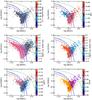 |
Fig. A.1 Same as Fig. 7 but using the Stel models. |
| In the text | |
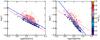 |
Fig. A.2 Same as Fig. 10 but using the Stel models. |
| In the text | |
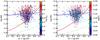 |
Fig. A.3 Same as Fig. 12 but using the Stel models. |
| In the text | |
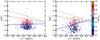 |
Fig. A.4 Same as Fig. 13 but using the Stel models. |
| In the text | |
Current usage metrics show cumulative count of Article Views (full-text article views including HTML views, PDF and ePub downloads, according to the available data) and Abstracts Views on Vision4Press platform.
Data correspond to usage on the plateform after 2015. The current usage metrics is available 48-96 hours after online publication and is updated daily on week days.
Initial download of the metrics may take a while.