| Issue |
A&A
Volume 691, November 2024
|
|
|---|---|---|
| Article Number | A16 | |
| Number of page(s) | 19 | |
| Section | Extragalactic astronomy | |
| DOI | https://doi.org/10.1051/0004-6361/202450762 | |
| Published online | 25 October 2024 | |
CLOUDY modeling suggests a diversity of ionization mechanisms for diffuse extraplanar gas
1
Space Physics and Astronomy Research Unit, University of Oulu, 90014 Oulu, Finland
2
Centre of Astrophysics Research, School of Physics, Astronomy and Mathematics, University of Hertfordshire, Hatfield AL10 9AB, UK
3
Departamento de Astrofísica, Universidad de La Laguna, 38200 La Laguna, Tenerife, Spain
4
Instituto de Astrofísica de Canarias, 38205 La Laguna, Tenerife, Spain
⋆ Corresponding author; This email address is being protected from spambots. You need JavaScript enabled to view it.
Received:
17
May
2024
Accepted:
13
September
2024
Abstract
Context. The ionization of diffuse gas located far above the energetic midplane OB stars poses a challenge to the commonly accepted notion that radiation from OB stars is the primary ionization source for gas in galaxies.
Aims. We investigated the sources of ionizing radiation, specifically leaking midplane H II regions and/or in situ hot low-mass evolved stars (HOLMES), in extraplanar diffuse ionized gas (eDIG) in a sample of eight nearby (17−52 Mpc) edge-on disk galaxies observed with the Multi Unit Spectroscopic Explorer (MUSE).
Methods. We constructed a model for the photoionization of eDIG clouds and the propagation of ionizing radiation through the eDIG using subsequent runs of CLOUDY photoionization code. Our model includes radiation originating both from midplane OB stars and in situ evolved stars and its dilution and processing as it propagates in the eDIG.
Results. We fit the model to the data using the vertical line ratio profiles of our sample galaxies, and find that while the ionization by in situ evolved stars is insignificant for most of the galaxies in our sample, it may be able to explain the enhanced high-ionization lines in the eDIG of the green valley galaxy ESO 544−27.
Conclusions. Our results show that while leaking radiation from midplane H II regions is the primary ionization source for eDIG, in situ evolved stars can play a significant part in ionizing extraplanar gas in galaxies with low star forming rates.
Key words: stars: AGB and post-AGB / HII regions / galaxies: ISM / galaxies: star formation
© The Authors 2024
 Open Access article, published by EDP Sciences, under the terms of the Creative Commons Attribution License (https://creativecommons.org/licenses/by/4.0), which permits unrestricted use, distribution, and reproduction in any medium, provided the original work is properly cited.
This article is published in open access under the Subscribe to Open model. This email address is being protected from spambots. You need JavaScript enabled to view it. to support open access publication.
1. Introduction
Diffuse ionized gas (DIG) is ubiquitous in late-type galaxies (e.g., Levy et al. 2019). Along with H II regions it constitutes the Hα-bright star-forming disk visible in narrow-band imaging and integral field unit (IFU) spectroscopy. DIG also extends beyond the classical star-forming disk, to great radial distances and far above the midplane (e.g., Dettmar 1990; Williams & Schommer 1993; Rand 1996; Watkins et al. 2018; Rautio et al. 2022).
The ionization of diffuse gas is mainly attributed to leaking radiation of massive young OB stars from midplane H II regions (Haffner et al. 2009; Weber et al. 2019). Leaky H II regions have been shown to be the primary source of ionization for extraplanar DIG (eDIG) at great heights above the midplane (Levy et al. 2019; Rautio et al. 2022). However, the emission spectrum of eDIG exhibits unique features such as the enhancement of [O III]λ5007 emission line (hereafter [O III]) that are difficult to explain without additional sources of ionization (e.g., Rand 1998; Collins & Rand 2001; Wood & Mathis 2004).
Many alternative sources of ionization for the eDIG have been investigated in addition to leaky H II regions. Among these alternative sources the most promise is shown by shocks (Dopita & Sutherland 1995; Collins & Rand 2001; Ho et al. 2014; Dirks et al. 2023) and hot low-mass evolved stars (HOLMES, Flores-Fajardo et al. 2011; Alberts et al. 2011; Zhang et al. 2017; Lacerda et al. 2018; Rautio et al. 2022). HOLMES are also called post asymptotic giant branch stars (post-AGB), as they include all stars in subsequent stages of evolution of the asymptotic giant branch, such as white dwarfs. They are much less luminous than the bright OB stars, but also much hotter, resulting in a harder ionizing spectrum, potentially explaining the enhancement of high ionization lines such as [O III]. While the total ionizing photon flux of HOLMES is several orders of magnitude less than that of OB stars, HOLMES are present in situ in the eDIG allowing a much greater portion of their radiation reach the eDIG (Stasińska et al. 2008).
We investigated the sources of eDIG ionization in a sample of five low-mass galaxies (ESO 157−49, ESO 469−15, ESO 544−27, IC 217, and IC 1553) in Rautio et al. (2022, hereafter Paper I), using Multi Unit Spectroscopic Explorer (MUSE) integral field spectroscopy and narrow-band imaging. While we found the primary ionization source for eDIG to be OB star radiation across the sample, we also found regions consistent with OB–HOLMES and OB–shock ionization in all of the sample galaxies. Our analysis consisted of photometry and spatially resolved emission-line diagnostics, and was mostly qualitative in nature. Here we extend the analysis to three more edge-on galaxies observed with MUSE (ESO 443−21, PGC 28308, and PGC 30591), and quantify the significance of HOLMES to the eDIG ionization by modeling its photoionization with version 23.00 of the CLOUDY code (Chatzikos et al. 2023).
Modeling the ionization of diffuse extended gas such as the eDIG poses unique challenges due to the large range of spatial scales involved. The eDIG can extend kiloparsecs both in the disk-plane and perpendicular to it, and at the same time exhibit porous and turbulent structure at the parsec scale as revealed by both observations (Dettmar 1990; Rand et al. 1990; Collins et al. 2000; Miller & Veilleux 2003; López-Cobá et al. 2019), and hydrodynamical simulations (Wood et al. 2010; Barnes et al. 2014, 2015; Vandenbroucke et al. 2018; Kado-Fong et al. 2020). The fine structure of the eDIG may include chimneys, holes and clouds, and it is mixed with neutral gas, as indicated by the presence of neutral emission lines such as [O I]λ6300 (hereafter [O I]) in eDIG spectra (e.g., Paper I). However, focusing on integrated properties allows us to create a model for the photoionization of eDIG that is able to reproduce the observed line ratios in our sample.
We describe the sample, the data, and the data analysis in Sect. 2. In Sect. 3, we present our model for the eDIG photoionization. We describe the best fit models for our sample galaxies and discuss the implications in Sect. 4. In Sect. 5, we discuss the caveats in our modeling approach and the nature of the eDIG. We finish with a summary and conclusions in Sect. 6.
2. Observations and data analysis
2.1. The sample
Our sample consists of eight edge-on galaxies observed by Comerón et al. (2019) with MUSE at the Very Large Telescope (VLT) of the European Southern Observatory (ESO), at Paranal observatory, Chile. The galaxies come from a subsample of the 70 edge-on disk sample of Comerón et al. (2012), that itself was derived from the Spitzer Survey of Stellar Structure in Galaxies (S4G; Sheth et al. 2010), selected to be observable from the Southern Hemisphere and to have an r25 < 60″ (as given in the HyperLEDA1 database; Makarov et al. 2014). This selection was done so that the region between the center of the target and its edge could be covered in a single MUSE pointing. The galaxies have relatively low masses, with stellar masses ranging from 4 × 10⁹ M⊙ to 4 × 10¹⁰ M⊙. Most of them also have clear separate thin and thick disks, while for two (ESO 443−21 and PGC 30591) the disk structure is less clear (Comerón et al. 2018). Some properties, including the masses and scale heights of thin and thick disks, of the sample galaxies can be found in Table 1.
Basic properties of our galaxy sample.
2.2. MUSE observations
For the MUSE observations, four 2624 s on-target exposures were taken per galaxy (three for IC 217), centered either on a single point on one side of the galaxy, or in the case of galaxies with smaller angular size (ESO 157−49 and IC 1553), on the center of the galaxy, with 90° rotations between exposures. The MUSE pipeline (Weilbacher et al. 2012) was used within the Reflex environment (Freudling et al. 2013) to reduce the data, while the Zurich Atmosphere Purge (ZAP; Soto et al. 2016) was used to clean the combined datacubes of sky residuals. To produce bins with S/N ∼ 50 in Hα the datacubes were tessellated with the Voronoi binning code by Cappellari & Copin (2003). Intensities of Hα, Hβ, [O III], [O I], [N II]λ6583, and [S II]λλ6717/31 (hereafter [N II], and [S II]) emission-lines were obtained with the Python version of the Penalized Pixel-Fitting code (pPXF; Cappellari & Emsellem 2004). The MUSE observations, data reduction, Voronoi binning, and the pPXF processing are described in detail in Comerón et al. (2019).
2.3. Hα photometry
For the star forming rates (SFR) and eDIG vertical profile parameters of most of our sample galaxies, we used the Paper I Hα photometry obtained from narrow-band data. However, we did not obtain Hα narrow-band imaging for the three galaxies that were not investigated in Paper I (ESO 443−21, PGC 28308, and PGC 30591). Instead we used MUSE data to obtain Hα photometry for these three galaxies by mapping the Voronoi-binned Hα emission-line intensity back to the MUSE grid.
To obtain the midplane H II-region scale height (hzH II) and the eDIG scale height (hzeDIG) we used the same process as described in detail in Paper I. Following is a brief explanation of the process: We first fit a line-of-sight integrated two-exponential disk model to the vertical profiles measured from the Voronoi-binned Hα maps, and obtained hzH II from the scale height of the thinner component. Then we fit the line-of-sight integrated two-exponential disk model to the Hα maps again, this time masking out the midplane up to  , and obtained hzeDIG from the scale height of the thicker component.
The main limitation of the MUSE data compared to the narrow-band data is the comparatively small field of view (FoV) of MUSE: most of the sample galaxies have a larger angular size parallel to the disk plane than the FoV of MUSE. This was a more significant issue for SFR measurement than the measurement of vertical profile averaged over the galaxy radius, as we obtained the SFRs from the integrated Hα intensities. To obtain SFRs from MUSE data that are comparable to the ones we obtained from narrow-band data in Paper I, we mirrored the Hα maps over the centers of the galaxies and replaced the missing data in each galaxy with its mirror over the z-axis. We then measured the integrated Hα flux of these mirrored Hα maps, correcting for extinction using color excess derived from Balmer decrement as
 (1)
(1)
where E(B − V) is the color excess, and k are obtained from the Calzetti et al. (2000) extinction law as
 (2)
(2)
where RV = 4.5 (Fischera & Dopita 2005), and λHα and λHβ are the wavelengths of Hα and Hβ. From the extinction-corrected Hα flux we calculated the Hα luminosity (LHα) using distances from Tully et al. (2008, 2016), and obtained the SFRs using the Hao et al. (2011) and the Murphy et al. (2011) calibrations as
 (3)
(3)
The SFRs and eDIG vertical profiles for ESO 443−21, PGC 28308, and PGC 30591, were obtained with incomplete spatial coverage due to the limited MUSE FoV. As such, the uncertainty of these measurements is high. To evaluate this uncertainty, we measured SFRs from the MUSE data in the same manner for the five galaxies for which we did have narrow-band data, and compared the extrapolated MUSE SFRs to the narrow-band SFRs. The largest difference between the MUSE SFRs and the narrow-band SFRs we found was MUSE SFR = 0.18 M⊙ yr−1 for IC 217 compared to narrow-band SFR = 0.25 M⊙ yr−1 (Rautio et al. 2022). The star-forming properties of our sample galaxies are gathered in Table 2.
Star-forming properties of our galaxy sample.
2.4. Metallicity
We produced Voronoi-binned metallicity maps for all galaxies in our sample using the emission-line intensities obtained with pPXF. We used the calibration of Dopita et al. (2016) to do this. We define metallicity here with the logarithmic oxygen–hydrogen ratio Z = 12 + log(O/H)2.
We measured vertical metallicity profiles from these Voronoi-binned metallicity maps by averaging the metallicity at each height. We only used bins with OB star dominated ionization in the averages, as Dopita et al. (2016) calibration was derived for H II-regions where ionization is caused by star formation. We determined the ionization source of the bins using the η-parameter (Erroz-Ferrer et al. 2019). The η-parameter is defined as a distance to the Kewley et al. (2001) and Kauffmann et al. (2003) starburst lines in the [NII]/Hα against [O III]/Hβ Baldwin-Phillips-Terlevich (BPT; Baldwin et al. 1981) diagram. Ionized gas having η < −0.5 indicates that it is located below the Kauffmann et al. (2003) line on the BPT diagram, and its ionization is dominated by radiation from OB stars, η > 0.5 indicates that it is located above the Kewley et al. (2001) line on the BPT diagram, and its ionization is dominated by other ionization sources, while −0.5 < η < 0.5 indicates mixed ionization between the two starburst lines.
In all of the galaxies, the measured metallicity profile exhibits a trend where it first decays exponentially as z increases, but after some height the metallicity either remains roughly constant or begins increasing again. The apparent enhancement of metallicity in the eDIG at large z is likely not a physical effect, but rather results from the gas density of the eDIG dropping below the limits where Dopita et al. (2016) calibration holds. We adopt a constant metallicity for the eDIG, and fit to the data a profile of the form
 (4)
(4)
where Z0 is the metallicity at the midplane, ZeDIG is the metallicity of the eDIG, and hzO/H is the scale height for the exponential decay of the metallicity between the midplane and the eDIG. The metallicity parameters for our sample are shown in Table 3.
Metallicity parameters for our galaxy sample.
3. Model for the photoionization of extraplanar diffuse ionized gas
3.1. Modeling scenario
We investigated here a simplified scenario where spherical clouds of diffuse gas, arranged in equidistant layers with increasing height over the midplane (z) and decreasing gas density, are ionized by OB star radiation originating from the midplane and HOLMES radiation originating from between the layers. Figure 1 shows a schematic view of our model. The radiation field of leaking midplane H II regions SOB(λ) and the radiation field of in situ HOLMES SHOLMES(λ), as well as the radiation field transmitted through the clouds St(λ), are shown in the schematic with colored arrows. We use “transmitted radiation” here to describe the sum of attenuated incident radiation and the emission of the cloud itself, following CLOUDY documentation nomenclature. The transmitted radiation field contains both the processed radiation field of midplane OB stars and the processed radiation field of HOLMES.
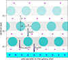 |
Fig. 1. Schematic of our model. The cyan shaded area indicates the star-forming disk and the large blue stars represent the OB stars within it. The gray shaded areas indicate the eDIG cloud layers, and the filled cyan circles show the eDIG clouds within them. The small purple stars represent the HOLMES between the cloud layers. The colored arrows indicate the source radiation fields of leaking midplane H II regions (SOB(λ); blue), HOLMES (SHOLMES(λ); magenta), and transmitted radiation (St(λ); cyan). Black arrows indicate the cloud diameter (d) and the layer separation (s). |
The individual eDIG clouds in our model have a constant gas density determined by their distance from the midplane, following an exponential decay. Each cloud layer also has a constant metallicity determined by Eq. (4). Our code also models the propagation of radiation between the layers taking into account the filling factor of the eDIG and average geometric dilution with the assumption that the clouds are located above the center of the galaxy disk. The determination of these parameters is explained Sects. 3.2 and 3.6.
We used version 23.00 of CLOUDY photoionization code (Chatzikos et al. 2023) to model the ionization of each cloud layer. CLOUDY is a 1-dimensional (1D) spectral synthesis code which inputs a radiation field into a cloud of interstellar gas and calculates the resulting physical condition in the cloud as well as the emitted and transmitted spectra in a plane-parallel or spherically symmetric geometry. In our model CLOUDY is ran once for each cloud layer using plane-parallel geometry and the radiation field leaking from midplane HII regions incident on the cloud surface IOB(λ), the incident radiation field from inter-layer HOLMES IHOLMES(λ), and the incident radiation field transmitted through clouds in the lower layers It(λ) is input, simulating an “average” eDIG cloud for that layer. We use I(λ) to denote the diluted radiation fields incident on the clouds and S(λ) to denote the undiluted source radiation fields3.
Our model is 1-dimensional, predicting the evolution of line ratios in the eDIG only as a function of z. The eDIG of real galaxies varies also along the disk plane. To take this into account we considered adopting a more complex modeling scenario where the model varies in coordinates (r, z), where r is the radial direction along the galaxy disk. However, we opted not to adopt this scenario due to several issues with it. Firstly, as we show in Paper I, the line-of-sight integrated radial Hα profiles of our sample galaxies are complex and cannot be decomposed into simple exponential disks. This would mean the radial dependence of OB star flux and gas properties would need to be left as free parameters. Secondly, as CLOUDY is used in our model to compute St(λ) and CLOUDY is a 1D code, the incident direction of radiation transmitted through the eDIG clouds is lost and thus the treatment of transmitted radiation would not be realistic in a 2-dimensional model. Thirdly, in a 2-dimensional model we would need to model individual clouds in each cloud layer separately, drastically increasing the computational load. Because of these reasons, we chose our 1D modeling approach. We consider the limitations of our approach throughout the following Sections.
3.2. Geometry
Before going into details about the ionization sources of our model and the parameters that we used for the CLOUDY runs, let us first examine the geometry of our scenario. The eDIG clouds in our model are arranged in grids within their layers so that the distance between a cloud and its four nearest neighbors within the layer is equal to the distance between cloud layers. In our scenario this distance s is related to the volume filling factor (fV) as follows:
 (5)
(5)
where dcloud = 100 pc is the diameter of the clouds, which is equal to the layer thickness. From this follows that the cloud cross-sections cover a fraction
 (6)
(6)
of each layer, where fS is the surface filling factor. The cloud layers are arranged so that the lower boundary of the first layer is at height z1, and the following layers are at heights zj = (j − 1)(s + dcloud)+z1, where j is the layer number.
As radiation propagates between the cloud layers, a fraction of the radiation field intensity is lost to ionizing the eDIG within the clouds and to geometric dilution. This affects the intensity of a radiation field incident to a cloud layer in the following way:
 (7)
(7)
where Sj(λ) is the source radiation field at layer j, Ii(λ) is the contribution to the incident radiation field at layer i, (1 − fS)|j − i| is the fraction of photons from layer j that reach layer i without striking any clouds, and gij is the geometric dilution factor between layers i and j. This applies for all i and j, regardless of the direction or source of the radiation.
The radii of the Hα disks of our galaxies are of similar order as the heights over midplane that eDIG reaches for our sample. This means that geometric dilution of the radiation is significant for our model, but not as strong as it is for a spherically symmetric system. We approximate the geometric dilution in our model as the dilution of the radiation field along the z-axis of a uniform disk source with radius R, which corresponds to the solid angle subtended by a disk with radius R at a perpendicular distance dz above the disk center
 (8)
(8)
Normalizing Eq. (8) so that it goes to unity in a plane-parallel scenario (R → ∞), we obtain
 (9)
(9)
as the geometric dilution factor.
3.3. Leaking radiation from H II regions
To model the radiation of the midplane population of OB stars, we used STARBURST99 (Leitherer et al. 1999) stellar population synthesis code. We adopted the Kroupa (2001) initial mass function (IMF), and the Geneva stellar tracks with solar metallicity and no rotation (Ekström et al. 2012). For the stellar model atmospheres, we used those of Pauldrach et al. (2001) and Hillier & Miller (1998), implemented into STARBURST99 by Smith et al. (2002). We assumed constant star formation and extracted the radiation field at 107 yr age, when it is stabilized.
Most midplane OB stars are located within H II regions, and it is likely that a significant portion of the flux that escapes midplane is processed by propagation through density bounded H II regions, hardening the radiation field above the midplane. To simulate this hardening of the radiation field, we performed preliminary CLOUDY runs of a density bounded H II regions for each galaxy in our sample, inputting the spectrum generated by STARBURST99, and taking as output the transmitted spectra from CLOUDY. We used as the H II regions 0.5 pc thick clouds with densities of 100 cm−3, illuminated by a radiation fields with hydrogen-ionizing photon surface fluxes Φ = 1013 cm−2 s−1. These CLOUDY parameters ensured a fully ionized, density bounded clouds with escape fractions that are in the high end of typical values derived for real H II regions ( ; Della Bruna et al. 2021; Teh et al. 2023). We chose to simulate a very “leaky” H II regions as they would be overpresented among the sources of the ionizing photons that reach the eDIG. Additionally, majority of radiation leakage in real H II regions most likely happens through empty holes, in which case the radiation field of the OB stars is not processed at all (Kimm et al. 2022). Thus, our model likely overestimates the hardening of OB star radiation field by partial absorption in the surrounding H II regions. This means that if the leaking OB star radiation in our model fails to reproduce the observed high-ionization line intensities in the eDIG, additional ionization sources must be present. We set the metallicities of the H II regions according to Z0 of the modeled galaxy.
We scaled the transmitted fields from the preliminary CLOUDY runs depending on the galaxy we were modeling to obtain the source radiation fields of the leaking midplane radiation SOB(λ). By following Eq. 7 we then obtained the incident radiation fields of the leaking midplane radiation for each cloud layer as
 (10)
(10)
where N is the number of layers.
3.4. In situ radiation from evolved stars
STARBURST99 does not include the radiation field of post-AGB stars, and as such is not well suited to modeling the spectra of HOLMES. We instead used PéGASE.3 spectral evolution synthesis code (Fioc & Rocca-Volmerange 2019) to produce the spectra of HOLMES for our model. We follow the approach of Flores-Fajardo et al. (2011), and take the spectrum of a coeval population of stars at an age of 10 Gyr as the spectral energy distribution of HOLMES. Instantaneous burst produces a realistic spectrum, as the integrated radiation field from all HOLMES in an old stellar population (older than 100 Myr) is nearly independent of its star formation history. We used Kroupa et al. (1993) IMF and solar metallicity for the PéGASE.3 run.
HOLMES are distributed throughout the thick disk and halo, unlike the OB stars that are primarily confined to the midplane, so HOLMES are inserted between the cloud layers in our model. Our model includes two HOLMES components, one follows the vertical profile of the thick disk, while the other is a flat background component truncated at the height of the final cloud layer with 10% of the mass of the thick disk component, representing the halo. Both components use the same PéGASE.3 spectrum. We scaled the intensity of the spectrum according to the thick disk mass of the galaxy we were modeling, and distributed it over the HOLMES components according to their vertical profiles. This gave us the radiation fields originating from each inter-layer HOLMES layer SHOLMES, j(λ). Then for each cloud layer i we calculated
 (11)
(11)
where IHOLMES, i(λ) is the sum of all the inter-layer HOLMES layer radiation fields incident at layer i.
3.5. Radiation transmitted through the eDIG clouds
The final component of the incident radiation field for each cloud layer in our model is the radiation transmitted through clouds in the lower layers. To obtain the transmitted radiation field incident at a given layer It, i(λ), we took the transmitted spectra given by CLOUDY for each lower layer St, j(λ) and computed the propagation of radiation as follows:
 (12)
(12)
where
![Mathematical equation: $$ \begin{aligned} {S\!}_{\mathrm{t} ,j}(\lambda ) = C_j \circ [I_{\mathrm{HOLMES} ,j}(\lambda ) + I_{\mathrm{OB} ,j}(\lambda ) + I_{\mathrm{t} ,j}(\lambda )], \;\; j = 1,\ldots ,N, \end{aligned} $$](/articles/aa/full_html/2024/11/aa50762-24/aa50762-24-eq15.gif) (13)
(13)
and Cj° is an operator representing the processing and hardening of the radiation field caused by a transmission through a cloud of layer j.
Our treatment of the transmitted radiation did not take into account the directionality of the HOLMES radiation. That is, the fact that HOLMES radiation originating from higher layers should be transmitted mostly towards the lower layers rather than back upwards. As CLOUDY does not differentiate between the origin of the photons in the transmitted spectrum, a more realistic approach taking into account the differing directions of the radiation field components is difficult to implement. However, this does not affect our results, as while the harder radiation field from HOLMES can have a significant effect on the ionization state of the eDIG, the HOLMES radiation makes up such a small fraction of the total radiation field that the exact distribution of the HOLMES radiation is not important. This is not an issue for the OB star radiation escaping from the midplane, as it all originates from below all of the eDIG cloud layers. We performed a more rigorous treatment that took into account the direction of the transmitted HOLMES radiation for models of two galaxies as described in Sect. 4.2.
3.6. Fitting the model to data
The input parameters for the model described above are SFR, escape fraction from the midplane (emp), radius of the galaxy (R), mass of the thick disk (MT), scale height of the thick disk (hzT), the ionization parameter at the surface of the first eDIG cloud (U1), the scale height of the gas density (hzn), the metallicity parameters (Z0, ZeDIG, and hzO/H), the filling factor of the eDIG (fV), the number of cloud layers (N), and the height of the first cloud layer (z1). Using these parameters our code computes the input parameters for the CLOUDY runs of each cloud layer and runs CLOUDY to obtain the predicted eDIG emission-line intensities at the height of each cloud layer.
We obtained MT, hzT, SFR, hzeDIG, and the metallicity parameters from Tables 1, 2, and 3, while for z1 we used the scale height of H II regions (hzH II) from Table 2, and for R we took the radius of the Hα disk measured by eye. For the escape fraction we used emp = 0.5. This is lower than eH II = 0.6 used in our models of density bounded H II regions as we assume that some H II regions are fully ionization bounded, or have holes directed only along the plane of the galaxy, and thus leak no radiation to the eDIG (Teh et al. 2023). The number of cloud layers was chosen for each model run so that the model extends to roughly equal height above the midplane as the MUSE data of the galaxy being modeled. This left U1 and fV as free parameters. We chose these as the free parameters because it is not possible to measure them from our MUSE data, yet they are crucial in determining the observed line ratios in the eDIG. The ionization state of the first layer strongly depends on U1, while the gas density, hzn, and fV are the primary determinants in the absorption and processing of the radiation field that occurs as it propagates through the eDIG, which in turn determines how the ionization structure changes as a function of z. The effects of U1 and fV on the model are illustrated by Figures 2 and 3, that show line ratio and η-parameter profiles for sets of model runs for ESO 544−27 where other parameters are kept constant but U1 and fV, respectively, are varied. Similar figures for the effect of other parameters on our model are shown in Appendix A.
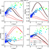 |
Fig. 2. Line ratio and η-parameter profiles for ESO 544−27 models with varying U1. The dots show the observed values, colored according to the η-parameter going from blue at low η to green at high η. The size of each dot is relative to the size of the corresponding Voronoi bin. The curves show the model predictions with the color of the curve corresponding with the model log U1, ranging from log U1 = −3.11. (black) to log U1 = −2.91 (red) with log U1 = 0.05 steps. All the models have fV = 0.17. |
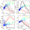 |
Fig. 3. Line ratio and η-parameter profiles for ESO 544−27 models with varying fV. The dots show the observed values, colored according to the η-parameter going from blue at low η to green at high η. The size of each dot is relative to the size of the corresponding Voronoi bin. The curves show the model predictions with the color of the curve corresponding with the model fV, ranging from fV = 0.11. (red) to fV = 0.23 (black) with fV = 0.03 steps. All the models have log U1 = −3.01. |
Our model uses the dimensionless ionization parameter, defined as U1 = Φ1/(n1c), where Φ1 is the total hydrogen ionizing photon flux at the surface of the first cloud and c is the speed of light, to calculate n1, the gas density of the first cloud. We chose to use U1 as an input parameter rather than n1 because the ionization structure of a low-density gas such as eDIG is primarily determined by U rather than n and Φ individually. As scale height of Hα emission is closely related to gas density scale height, we used the scale height of the disturbed eDIG (hzeDIG) to determine hzn. Due to geometric dilution of the ionizing radiation field, the Hα intensity declines faster than the gas density. Seon (2009) constructed two exponential gas disk models (one with hzn = 1 kpc and one with hzn = 1.5 kpc) for the face-on spiral M 51, and let the disks be ionized by radiation leaking from observed midplane HII regions. Their modeling produced vertical Hα profiles consisting of two exponential components with the thicker component having a scale height ∼30% smaller than the model hzn. This thicker exponential component of the Hα profile corresponds with our measured hzeDIG, so following this we used hzn = 1.3hzeDIG for our models. An example of the resulting density profile is shown for a model run of ESO 544−27 in Fig. 4 alongside an HOLMES number-density profile.
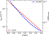 |
Fig. 4. Density profile of gas and HOLMES for an ESO 544−27 model. Red dots indicate the cloud layers and blue stars indicate the HOLMES layers. The connecting solid curves plot the densities. For HOLMES, the relative number density defined as the fraction of HOLMES at each layer is plotted. The model parameters are log U1 = −3.01, which is used to determine the density at midplane (see text), and the scale heights of the gas density (hzn = 0.79 kpc), and HOLMES number density (hzT = 0.67 kpc). The gas density of the clouds follows an exponential profile, while the HOLMES number density profile has an exponential component and a constant component with 10% of the mass of the exponential component ((n/N)HOLMES = 2.5 × 10³). |
STARBURST99 gives the total number of hydrogen ionizing photons emitted each second by a population with a certain SFR. With our parameters, it gave 1053.12 s−1 for SFR of 1 M⊙ yr−1. By multiplying this number with the SFR of each galaxy, we obtained the total number of hydrogen ionizing photons emitted by that galaxy. Nearly all of these photons are produced by the midplane OB stars, with a fraction equal to emp escaping the surrounding HII regions and reaching the eDIG. Dividing this number by 2πR2 gives the surface flux of hydrogen ionizing photons of OB stars at midplane (ΦOB), assuming that the OB stars are evenly distributed in the Hα disk and that half of the escaping photons are directed above the midplane and half of them below the midplane. Inputting ΦOB and the STARBURST99 spectrum into the preliminary H II region CLOUDY runs described in Sect. 3.3 yielded SOB(λ).
To obtain the total number of hydrogen ionizing photons emitted each second by HOLMES, we integrated the population-mass-normalized HOLMES spectrum given by PéGASE.3 and multiplied it with MT of each galaxy. We then divided this number by 2πR2 to obtain the total ΦHOLMES produced by HOLMES on one side of the midplane, and distributed this between the cloud layers as described in Sect. 3.4 obtaining SHOLMES, j(λ).
For our initial set of models we selected the values for our free parameters U1 and fV by hand. We did this by testing different values of U1 and fV and comparing by eye the predicted vertical profiles of [NII]/Hα, [S II]/Hα, and [OIII]/Hβ to the observed line ratio profiles until we obtained a satisfactory match between them. We examine these models in detail in Sect. 4. We did not attempt more rigorous numerical fitting for these initial models as our goal was to investigate the general validity of the proposed schema of ionization of the eDIG by leaking OB star radiation and HOLMES, rather than finding exact physical parameters of the eDIG. We performed χ2 minimization on a grid of more detailed models for two of the galaxies as described in Sect. 4.2.
4. Results
4.1. Ionization of the eDIG in the sample galaxies
Figures 5, 6, 7, and 8. show the vertical profiles of the [N II]/Hα, [SII]/Hα, [OI]/Hα, and [OIII]/Hβ line ratios for our sample galaxies. The blue and yellow dots are the observed values from MUSE data, with each dot corresponding to a single Voronoi bin, and the size of the dot corresponding with the size of the Voronoi bin. The blue dots are from Voronoi bins where the ionization is dominated by OB star radiation, while the yellow dots are from bins with mixed ionization or ionization dominated by other sources. We did this separation using the η-parameter, so that blue dots have η < −0.5 and yellow dots have η > −0.5. The red curves correspond to our model runs. The black curves are the same as the red curves, only with HOLMES turned off. When choosing the free parameters, we only considered the bins with OB star dominated ionization (η < −0.5, blue dots). We did this because some of the galaxies in our sample exhibit clear shock ionization (Paper I), and here we are only modeling photoionization. In particular ESO 157−49 and IC 1553 exhibit clear bimodal distributions in their vertical [N II]/Hα profiles, and the branches with enhanced η correspond spatially with biconical outflows visible in the η-parameter and velocity dispersion maps. These branches with enhanced η are most likely caused by shock ionization as a superbubble breaks out from the midplane (for IC 1553 see Dirks et al. 2023), and as such we ignored them when fitting our photoionization model to ESO 157−49 and IC 1553.
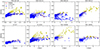 |
Fig. 5. [N II]/Hα vertical profiles for our sample galaxies. The blue dots show observed values from Voronoi bins with OB star dominated ionization (η < −0.5). The yellow dots show observed values from Voronoi bins with mixed ionization or ionization dominated by other sources (η > −0.5). The size of each dot is relative to the size of the corresponding Voronoi bin. The solid red curve shows our model for the galaxy in question. The dashed black curve is the same model as the red curve but with HOLMES turned off. The contribution from HOLMES to the ionizing radiation is insignificant for our models when fitting OB star dominated ionization. |
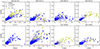 |
Fig. 7. Same as Fig. 5 but for [O I]/Hα. The [O I]/Hα line ratio is poorly fit because [O I] is a collisionally excited line of neutral oxygen, and as such is only produced by partly ionized and neutral gas, while our model emission lines are dominated by fully ionized gas. |
Figure 9 shows the contribution of different ionization sources to the ionizing radiation in the models. The transmitted component curve in the figure (orange dot-dashed line) includes both the transmitted OB star radiation and the transmitted HOLMES radiation. For all of the galaxies ΦHOLMES ≤ 10−2ΦOB for the first cloud, with the contribution of HOLMES increasing slowly with z and reaching ΦHOLMES ≈ 10−1ΦOB at most (for ESO 544−27). The contribution of transmitted radiation depends on whether the eDIG clouds are fully ionized and density bounded or ionization bounded. For ESO 469−15 and PGC 28308 models all of the eDIG clouds are ionization bounded, and very little radiation is transmitted, resulting in very low Φt at all z. For ESO 544−27 and IC 217 models all of the eDIG clouds are density bounded, and significant portion of the radiation is transmitted at every layer. For ESO 157−49, ESO 443−21, IC 1553, and PGC 30591 eDIG clouds near midplane are ionization bounded, while as z increases and density goes down, upper eDIG clouds become density bounded, resulting in a clear transition in the Φt profile where it increases significantly when density becomes low enough to allow for the full ionization of the eDIG clouds.
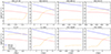 |
Fig. 9. Contributions of different components to the ionizing radiation for the best fit models. Blue solid lines shows the contribution from midplane OB stars, red dashed line shows the contribution from HOLMES, and the orange dot-dashed line shows the contribution of transmitted radiation. The transition from ionization bounded clouds to density bounded clouds is visible as a steep upturn in the contribution of transmitted radiation. |
The models were chosen to best reproduce [NII]/Hα, [SII]/Hα, and [OIII]/Hβ simultaneously, ignoring [OI]/Hα, as no model was able to simultaneously reproduce all of the observed line ratios. This is because [OI] is a collisionally excited line of neutral oxygen, and as such is only produced by partly ionized and neutral gas. Our CLOUDY models do not extend far into neutral gas, and as such even in the models with only ionization bounded eDIG clouds the majority of the emitted radiation is produced in the fully ionized parts of the clouds. In the real complex 3D environment of the eDIG there exist simultaneously fully ionized, partly ionized, and neutral gas. Thus, as we are fitting the line ratios originating from fully ionized gas, our models underestimate [OI]/Hα. As an example of a model that reproduces [OI]/Hα well, Fig. 10 shows the line ratio profiles for an ESO 157−49 model where ΦOB has been reduced to 2% of our prediction using SFR and STARBURST99 modeling. In this model the transition region to neutral gas, where [OI] is produced, is of comparable size to the fully ionized part of the cloud. For this model we kept the density of the gas equal to the best fit model by setting log U1 = −4.51. Other parameters of this model are the same as the best fit model.
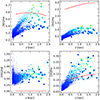 |
Fig. 10. Line ratio profiles for ESO 157−49 model with 2% ΦOB. The dots show the observed values, colored according to the η-parameter going from blue at low η to green at high η. The size of each dot is relative to the size of the corresponding Voronoi bin. The red curve shows the model predictions. This model predicts the [O I]/Hα line ratio well, but fails to predict any of the other line ratios. The log U1 = −4.51 and other parameters are same as in the best fit model. |
We were unable to simultaneously reproduce both of the observed [NII]/Hα and [SII]/Hα for some of the galaxies in our sample, particularly IC 217 and PGC 28308 (see Figs. 5 and 6). This is most likely because of the simplified approach to the elemental abundances in our models. We are using the preset interstellar medium “ISM” abundances in CLOUDY, and only scaling the elements heavier than helium to match the observed metallicity (12 + log(O/H)). This does not take into account any differences in nitrogen and sulfur abundances, which are important to accurately model the [NII] to [SII] ratio. This is not an issue for [OIII], as the second ionization potential of oxygen is significantly higher than the first ionization potentials of [N II] and [SII] (35.1 eV, 14.5 eV, and 10.4 eV, respectively), and as such the ratio of [OIII] to [NII] or [SII] is less dependent on elemental abundances and more on the shape and intensity of the ionizing spectrum.
Table 4 shows the chosen parameters for each galaxy. The gas densities of the first cloud layers in our models range from 0.2 cm−3 to 1 cm−3. These are somewhat high when compared to the measured DIG densities in Milky Way (0.34 ± 0.06 cm−3 at midplane; Gaensler et al. 2008). However, for all models the gas density falls below 0.3 cm−3 higher in the eDIG, where our simple 1D modeling scenario works best. The chosen fV for our galaxies on the other hand are lower than the measured fV for Milky Way (∼0.2; e.g., Reynolds 1991). Similar results are found in studies of face-on galaxies, that extremely low fV are required to explain the propagation of OB star radiation and ionization of DIG within the midplane (Seon 2009; Belfiore et al. 2022; Watkins et al. 2024).
Model parameters.
4.2. Contribution of HOLMES to the eDIG ionization
Figures 5, 6, 7, and 8 show very little difference between the models with and without HOLMES. This is to be expected when modeling OB star dominated ionization. In Paper I we suggest that HOLMES could be responsible for the enhanced η-parameter in the eDIG in ESO 544−27. ESO 544−27 has a relatively massive thick disk and relatively low SFR when compared to the other galaxies in our sample, meaning that the HOLMES contribution to its ionization budget is much larger, especially in the eDIG. To investigate this we constructed an alternative high-ΦHOLMES model for ESO 544−27, this time attempting to fit the Voronoi bins with mixed ionization source (η > −0.5). For this model we set the HOLMES mass to 1.5 × MT, ΦOB to half of what our STARBURST99 models predict, and emp = 0.2. These alternate parameters result in much higher ΦHOLMES compared to ΦOB, while still being reasonable considering the large uncertainties in determining the photon fluxes of our models. We also left hzn as a free parameter, as we found that it is the only parameter that can move the peak of the [NII]/Hα and [S II]/Hα line ratio profiles to higher z.
Since the HOLMES contribution to the transmitted radiation field is much higher for the high-ΦHOLMES ESO 544−27 model than to any of the previous models, we adopted a more rigorous treatment for the transmitted radiation field. To do this we followed an iterative approach, where first for each cloud layer we divided the output transmitted radiation field to two components with intensity ratio equal to the input ΦHOLMES/ΦOB, then we further divided the component related to ΦHOLMES into upwards component and downwards component, which were proportional to the amount of HOLMES below the cloud layer and above the cloud layer, respectively. We then used the downward HOLMES component of the transmitted radiation field as an additional input in a re-run of the model. This essentially modified Eq. (12) for the re-run into
 (14)
(14)
where aj is the fraction of HOLMES above layer j, St, j0(λ) is the source transmitted radiation field from the first run, and It, i1(λ) and St, j1(λ) are the incident and source transmitted radiation fields of the second run. We tested further iterations and found that the model converges quickly and the changes to the line ratio profiles are indistinguishable by eye after the first iteration.
We constructed a 1100 model grid of high-ΦHOLMES ESO 544−27 models by varying hzn from 0.8 kpc to 1.8 kpc in 0.1 kpc steps, log U1 from −3.35 to −2.90 in steps of 0.5, and fV from 0.05 to 0.32 in steps of 0.03. We found the best fit model by minimizing the χ2 defined as
![Mathematical equation: $$ \begin{aligned} \chi ^2 = \sum ^{3n} \frac{[I_{\rm 1, obs}/I_{\rm 2, obs} - I_{\rm 1, model}/I_{\rm 2, model}]^2}{\sigma _{1,2}^2}, \end{aligned} $$](/articles/aa/full_html/2024/11/aa50762-24/aa50762-24-eq17.gif) (15)
(15)
where n is the number of Voronoi bins with η > −0.5, I1, obs/I2, obs are the observed [NII]/Hα, [SII]/Hα, and [OIII]/Hβ line ratios of those Voronoi bins, I1, model/I2, model are the model values for those line ratios, and σ1, 22 are the uncertainties of the line ratios, defined as
![Mathematical equation: $$ \begin{aligned} \sigma _{1,2}^2 = \left(\frac{I_{\rm 1, obs}}{I_{\rm 2, obs}}\right)^2 \left[\left(\frac{\sigma _1}{I_{\rm 1, obs}}\right)^2 + \left(\frac{\sigma _2}{I_{\rm 2, obs}}\right)^2\right]. \end{aligned} $$](/articles/aa/full_html/2024/11/aa50762-24/aa50762-24-eq18.gif) (16)
(16)
We restricted the fitting to Voronoi bins with η > −0.5 because we are interested in finding a model that reproduces the parts of eDIG with mixed ionization sources. Without this restriction χ2 would be heavily weighed by values near the midplane due to the better signal-to-noise and larger number of Voronoi bins therein.
We found the best fit with hzn = 1.7 kpc, fV = 0.11, and log U1 = −3.30. The goodness of the fit is χ2/ν = 39, which is normalized by the number of degrees of freedom4. In order to verify that HOLMES are required to find a good fit, we also constructed a 1100 model grid of ESO 544−27 models with otherwise the same parameters, but HOLMES turned off. For this grid we found the best fit with hzn = 1.6 kpc, fV = 0.11, and log U1 = −3.30, with χ2/ν = 75. The best fit models from both of these grids are shown in Fig. 11. As χ2/ν is nearly twice as large for the best fit model without HOLMES compared to the high-ΦHOLMES best fit model, and it is visually clear from Fig. 11 that the high-ΦHOLMES best fit model reproduces η and the line ratios much better than the best fit model without HOLMES, we confirm that including HOLMES improves the fit for ESO 544−27.
Another galaxy in our sample with a similar enhancement of the η-parameter throughout the eDIG as ESO 544−27 is PGC 28308. We constructed a similar high-ΦHOLMES and no HOLMES model grids for it by varying hzn from 1.0 kpc to 2.0 kpc in 0.1 kpc steps, log U1 from −3.35 to −2.90 in steps of 0.5, and fV from 0.05 to 0.32 in steps of 0.03. The high-ΦHOLMES models also had 1.5 × MT HOLMES mass, halved ΦOB, emp = 0.2, and used the more rigorous treatment of the transmitted radiation as described above. By minimizing χ2 we again found the best fit high-ΦHOLMES model for η > −0.5 with hzn = 1.2 kpc, fV = 0.14, and log U1 = −3.10, and best fit model without HOLMES for η > −0.5 with hzn = 1.1 kpc, fV = 0.14, and log U1 = −3.10. However, for this high-ΦHOLMES fit χ2/ν = 156, which while higher than the best fit no HOLMES model (χ2/ν = 175), is much worse than χ2 of the ESO 544−27 best fit models, and the model fails to reproduce the high η-parameter in the eDIG of PGC 28308. In order to find a better fit we constructed an extreme-ΦHOLMES PGC 28308 model grid with otherwise the same parameters as the high-ΦHOLMES PGC 28308 model grid except with increased HOLMES mass to 4 × MT and quartered ΦOB. We found for the best fit extreme-ΦHOLMES PGC 28308 model hzn = 1.9 kpc, fV = 0.14, and log U1 = −3.20, and while this model is able to reproduce the observed high η-parameter in the eDIG of PGC 28308, it is still not very well fit with χ2/ν = 167. The best fit models for PGC 28308 are shown in Fig. 12.
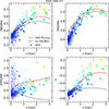 |
Fig. 11. Line ratio and η-parameter profiles for the best fit alternative high-ΦHOLMES ESO 544−27 model (see text). The dots show the observed values, colored according to the η-parameter going from blue at low η to green at high η. The size of each dot is relative to the size of the corresponding Voronoi bin. The solid red curve shows the best fit model including HOLMES (χ2/ν = 39) while the dashed black curve shows the best fit model without HOLMES (χ2/ν = 75). The best fit values for the models including HOLMES are hzn = 1.7 kpc, fV = 0.11, and log U1 = −3.30, while the best fit values for the models without HOLMES are hzn = 1.6 kpc, fV = 0.11, and log U1 = −3.30. The high-ΦHOLMES model reproduces the observed η > −0.5 in the eDIG of ESO 544-27. |
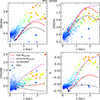 |
Fig. 12. Line ratio and η-parameter profiles for the best fit PGC 28308 models. The dots show the observed values, colored according to the η-parameter going from blue at low η to green at high η. The size of each dot is relative to the size of the corresponding Voronoi bin. The solid red curve shows the best fit high-ΦHOLMES model (χ2/ν = 156), the dash-dot magenta curve shows the best fit extreme-ΦHOLMES model (χ2/ν = 167), and the dashed black curve shows the best fit model without HOLMES (χ2/ν = 175). The best fit values are hzn = 1.2 kpc, fV = 0.14, and log U1 = −3.10 for the high-ΦHOLMES model, hzn = 1.9 kpc, fV = 0.14, and log U1 = −3.20 for the extreme-ΦHOLMES model, and hzn = 1.1 kpc, fV = 0.14, and log U1 = −3.10 for the model without HOLMES. The reasonable high-ΦHOLMES model fails to reproduce the high η-parameter in the eDIG of PGC 28308, and a model with unrealistically high ΦHOLMES/ΦOB is required to do so. |
In order to determine quantitatively how high HOLMES flux is required to produce the observed η-parameter in the eDIG of ESO 544−27 and PGC 28308 we looked into the relative contributions of different ionization sources in our models. These are plotted in Fig. 13. The left panels show the contributions of different components to the ionizing radiation in the eDIG of our high-ΦHOLMES models, with the transmitted radiation shown separately for OB stars and HOLMES. These plots show that for the models that are capable of reproducing the observed enhanced η-parameter in the eDIG of ESO 544−27 and PGC 28308 (high-ΦHOLMES ESO 544−27 model and the extreme-ΦHOLMES PGC 28308 model), ΦOB is lower than ΦHOLMES or Φt at high z. However, this is also true for the high-ΦHOLMES PGC 28308 model that cannot reproduce the observed enhanced η-parameter at high z. Also, for the high-ΦHOLMES ESO 544−27 model, Φt is still an order of magnitude higher than ΦHOLMES at high z, meaning that most of the ionizing flux there still originates from the midplane. This would seem to suggest that both the radiation from in situ HOLMES and the procession of midplane radiation by intermediate clouds contribute to the hardening of the radiation field and enhancement of the η-parameter observed in eDIG.
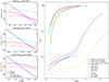 |
Fig. 13. Contributions of the different ionization sources over z for the models with enhanced ΦHOLMES. Top-left panel: contributions of different components to the ionizing radiation for the high-ΦHOLMES ESO 544−27 model. The blue solid line shows the contribution from midplane OB stars, the red solid line shows the contribution from HOLMES, and the cyan and magenta dashed lines show the contribution of transmitted emission from midplane OB stars and HOLMES, respectively. Middle-left panel: same as top-left panel but for the high-ΦHOLMES PGC 28308 model. Bottom-left panel: same as top-left panel but for the extreme-ΦHOLMES PGC 28308 model. Right panel: relative contribution of combined HOLMES radiation and transmitted radiation for all of our models ϕhard = (ΦHOLMES + Φt)/Φ. The thick cyan curve shows ϕhard for the high-ΦHOLMES ESO 544−27 model. The thick dash-dot red curve shows ϕhard for the high-ΦHOLMES PGC 28308 model. The thick solid red curve shows ϕhard for the extreme-ΦHOLMES PGC 28308 model. The dashed curves show ϕhard for the original models. Only models where ϕhard approaches unity are able to produce η > −0.5 in the eDIG. |
The right panel of Fig. 13 shows the combined relative contribution of HOLMES and transmitted radiation to the ionizing radiation in the eDIG of all our models ϕhard = (ΦHOLMES + Φt)/Φ. The combined relative HOLMES and transmitted radiation contribution approaches unity in the eDIG of the high-ΦHOLMES ESO 544−27 model, and the high-ΦHOLMES and extreme-ΦHOLMES PGC 28308 models, while remaining below 0.6 for all other models. This suggests that the contribution of unprocessed midplane radiation to the ionization of eDIG must be vanishingly low where η > −0.5.
5. Discussion
5.1. Model uncertainties and limitations
Whether or not our composite leaking H II region and in situ HOLMES photoionization model can reproduce the enhanced η-parameter present in the eDIG of ESO 544−27 and PGC 28308 depends primarily on the ΦHOLMES/ΦOB ratio. This ratio is sensitive to choices made during stellar population modeling as well as to SFR and MT measurements. To gain an understanding of the sensitivity of the STARBURST99 OB star population model to different parameters we tested the effect of different IMFs and evolutionary tracks to the predicted ΦOB. We found that a model with steeper IMF for massive stars (α = 2.7 rather than the standard Kroupa α = 2.3), predicts ΦOB one third of our adopted model. As low SFR environment may give rise to a steeper IMF (e.g., Pflamm-Altenburg & Kroupa 2008; Rautio et al. 2024), we may be overestimating ΦOB for ESO 544−27. While most of the alternative evolutionary tracks available in STARBURST99 did not produce large differences to the predicted ΦOB, using the Geneva stellar tracks with rotation (Ekström et al. 2012) caused a ∼70% increase in ΦOB. The uncertainties in our SFR measurements are demonstrated by the differences we found between the measurements done using MUSE data and the measurements done using narrow-band data, the largest of which was ∼30% for IC 217. Additionally, Hα alone as a SFR indicator tends to underpredict the true SFR for low luminosity galaxies (Lee et al. 2009). The thick disk masses were obtained by fitting the 3.6 μm vertical surface-brightness profiles of each galaxy with the superposition of two isothermal disks in a hydrostatic equilibrium, and assuming a ratio of thick disk mass-to-light ratio to thin disk mass-to-light ratio of 1.2. This procedure gives a typical uncertainty of ∼50% to the resulting MT (Comerón et al. 2012). Considering these uncertainties we determine that the parameters we used for the high-ΦHOLMES ESO 544−27 model are reasonable, while it is unlikely that ΦHOLMES/ΦOB is high enough in PGC 28308 to explain its enhanced eDIG η-parameter.
Due to the one dimensional nature of our models, they fail to capture the nonlinear effects of the clumpy, turbulent 3D environment in which real eDIG clouds reside. This is evident from our inability to simultaneously reproduce the observed neutral [O I] line and the observed ionized lines ([N II], [S II], and [O III]). This limitation is imposed by the spatial and line-of-sight integration required in the Voronoi binning of our MUSE data that we use to fix many of the model parameters. Single Voronoi bin may contain, and its observed emission lines may originate from, ionized gas in many different conditions. Indeed, more detailed modeling of the small scale structure of the eDIG by post-processing density grids from magnetohydrodynamic (MHD) simulations has revealed the temporal and spatial variability of the density and ionization structure possible in eDIG and shown that turbulence and superbubbles can produce low-density channels through which ionizing photons can travel far above the midplane and photoionize eDIG (Barnes et al. 2014, 2015; Vandenbroucke et al. 2018; Kado-Fong et al. 2020). These models reproduce the vertically stratified multiphase ISM observed in the solar neighborhood with a few pc resolution, which is crucial in constructing an holistic model for the ionization of eDIG. However, none of these models based on MHD density grids have to our knowledge included HOLMES, and they struggle to reproduce the observed line ratios in eDIG. Additionally, recent time-dependent radiation-hydrodynamic simulations by McCallum et al. (2024) have shown the significant effect that HOLMES can have on the eDIG ionization in simulations of the solar neighborhood ISM. The next step in modeling eDIG would be the inclusion of ionizing radiation from HOLMES and rigorous photoionization modeling in MHD density grid post-processing. Nevertheless, our 1D models are well suited to predicting the average integrated behavior of [N II], [S II], and [O III] lines as a function of z, as the primary determinants of these lines, ΦOB, ΦHOLMES, and n, follow in real galaxies on average the same relations as they do in our models.
5.2. Nature of eDIG ionization
Our results suggest that a combination of OB star radiation escaping the midplane H II regions and in situ HOLMES radiation is capable of producing the enhanced high-ionization lines and η-parameter observed in the eDIG of galaxies such as ESO 544−27. However, this seems to require a HOLMES population that is sufficiently massive in relation to the OB star population, indicating a low-SFR galaxy. ESO 544−27 seems to be one such galaxy, as it is not part of the main sequence of star forming galaxies, but rather is in the green valley (Paper I). We plot the relative contribution of ΦHOLMES to the ionizing radiation incident at the last cloud layer in the original models against the specific SFR (sSFR) of each galaxy in Fig. 14. We define the sSFR as sSFR = SFR/(Mt + MT + MCMC), where Mt and MCMC are the masses of the thin disk and central mass concentration, respectively, both from Comerón et al. (2018). Using the definition of Hsieh et al. (2017) that star-forming galaxies have sSFR > 10−10.6 yr−1, PGC 28308 also falls into the green valley. However, it also has the least massive thick disk in relation to its thin disk in our sample, and the high-ionization lines and the η-parameter are even more enhanced in the eDIG of PGC 28308 than the eDIG of ESO 544−27. Due to this, it seems unlikely that HOLMES and leaky H II regions could alone explain the ionization state in the eDIG of PGC 28308.
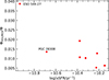 |
Fig. 14. Relative contribution of HOLMES to the model ionizing radiation in eDIG against galaxy sSFR. ESO 544−27 and PGC 28308 are labeled. There is a clear anti-correlation between sSFR and ΦHOLMES/Φ (ρ = −0.79, p = 0.02). |
Figure 14 also demonstrates the anti-correlation between ΦHOLMES/Φ in the eDIG and sSFR in our sample. We calculated the Spearman rank correlation coefficient for this relation ρ = −0.79, and obtained p = 0.02 as the p-value for the null hypothesis of no correlation. Due to the short lifetimes of OB stars (∼10 Myr), galaxies with low sSFR have relatively few OB stars active at any given moment compared to high-sSFR galaxies. HOLMES on the other hand have lifetimes larger than the age of the universe, and as such their numbers are independent of present day sSFR. Thus, it arises naturally that the photoionization of the eDIG by HOLMES is more significant in low-sSFR galaxies.
The case of eDIG ionization by a combination of in situ HOLMES radiation and leaking midplane H II region radiation was first quantitatively explored by Flores-Fajardo et al. (2011), using a grid of photoionization models to reproduce the observed line ratios in the edge-on spiral galaxy NGC 891. In their models the propagation and transmission of radiation through the eDIG was not simulated, instead ΦHOLMES was fixed and ΦOB was varied, with the different values of ΦOB representing different amounts of absorption suffered by the escaping midplane OB star radiation. They concluded that when restricting to solar metallicity, models that fit the observations become dominated by HOLMES as z increases. NGC 891 does have significantly enhanced [N II], [S II], and [O III] in its eDIG similarly to ESO 544−27 and PGC 28308 (Otte et al. 2001), but unlike them it has a relatively high SFR of 5.2 M⊙ yr−1 and low MT of 3 × 10¹⁰ M⊙ (Flores-Fajardo et al. 2011). In fact it is likely that our model, if applied to NGC 891, would be able to reproduce the observed line ratios only when assuming a HOLMES population much more massive than that suggested by the MT of NGC 891. This is because our model takes into account the dilution and absorption of HOLMES radiation unlike that of Flores-Fajardo et al. (2011), significantly reducing the incident ΦHOLMES. As an example, for our high-ΦHOLMES ESO 544−27 model the sum of the incident ΦHOLMES and the transmitted incident ΦHOLMES for each cloud layer ranges from 2.5 to 25 times smaller than the total source ΦHOLMES, which (Flores-Fajardo et al. 2011) used as the incident ΦHOLMES in their models. Therefore (Flores-Fajardo et al. 2011) may be overestimating ΦHOLMES by more than an order of magnitude.
If combination of in situ HOLMES and escaping midplane radiation is incapable of producing the ionization state in the eDIG of such galaxies as PGC 28308 and potentially NGC 891, an additional ionization source is required. Outflow driven shock ionization is one candidate. While PGC 28308 does not have clear biconical outflows like ESO 157−49 and IC 1553, the enhanced η-parameter and in fact the eDIG altogether as detected by MUSE, is concentrated above the center of PGC 28308. Moreover, as the MUSE data does not cover the full radial extent of the galaxy, we do not have the whole picture of the eDIG morphology. The ionization state in PGC 28308 eDIG could be caused by an advanced stage of a large superbubble breakout, or combination of multiple smaller superbubbles breakouts. Figure 15 shows the η-parameter map, ionized gas velocity dispersion (σ) map, the Hα equivalent width map, and the Veilleux-Osterbrock (VO; Veilleux & Osterbrock 1987) suite of diagnostic diagrams for PGC 28308. The slight enhancement of velocity dispersion in PGC 28308 eDIG could be caused by shocks. The low Hα equivalent width (EW(Hα) < 14 Å) in PGC 28308 eDIG indicates that OB star radiation alone cannot be responsible for its ionization. Similar situation may contribute to the enhanced line ratios in NGC 891 eDIG, as evidence of a superbubble has been found therein (Yoon et al. 2021).
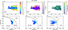 |
Fig. 15. Emission-line properties for PGC 28308. (a): η-parameter map. (b): velocity dispersion map. (c): logarithmic EW(Hα) map. The lower limit of the OB-star-dominated ionization (EW(Hα) = 14 Å) is contoured in black. (d)–(f): VO diagrams. The solid line is the Kewley et al. (2001) extreme starburst line, the dashed line in (d) is the Kauffmann et al. (2003) empirical starburst line, and the dash-dot lines in (e) and (f) are the Kewley et al. (2006) Seyfert and low-ionization narrow emission-line region (LINER) demarcation line. The colors in the VO diagrams correspond to the colors in the η-parameter map. While there is no clear biconical morphology in the η-parameter map, the concentration of the eDIG over the center of the galaxy could hint at ionization by outflow driven shocks. Similar figures for ESO 443−21 and PGC 28308 are found in Appendix B. |
Our small sample of eight edge-on galaxies gives likely examples of at least three distinct scenarios of eDIG ionization:
-
For half of the galaxies (ESO 443−21, ESO 469−15, IC 217, and PGC 30591) their eDIG emission can be satisfactorily explained with just photoionization by leaking radiation from midplane H II regions.
-
To explain the ionization state of the eDIG of the green valley galaxy ESO 544−27, photoionization by in situ HOLMES is required in addition to photoionization by leaking H II regions.
-
In ESO 157−49, IC 1553, and potentially PGC 28308, superbubble driven shock ionization causes harder ionization and elevates the η-parameter in certain parts of the eDIG.
All three scenarios are also supported by other recent work. Levy et al. (2019) finds photoionization by leaking H II regions to account for 90% of the eDIG ionization in their sample of 25 edge-on galaxies selected from the Calar Alto Legacy Integral Field Area (CALIFA) survey, while Lacerda et al. (2018) finds four edge-on galaxies where above and below the plane all emission indicated photoionization dominated by HOLMES also from CALIFA data. Both Levy et al. (2019) and Lacerda et al. (2018) use low Hα equivalent width as an indicator of HOLMES ionization, indicating that the differences between their results come indeed from differences between their samples rather than differences between their methodologies. Also from CALIFA López-Cobá et al. (2019) finds evidence of outflows in 17 edge-on galaxies. Similar composite ionization models with leaking H II regions and HOLMES as ionization sources are found to also work well for DIG in face-on galaxies (Belfiore et al. 2022).
6. Summary and conclusions
We constructed a self-consistent5 model for the photoionization of eDIG by leaking midplane H II regions and in situ HOLMES using the CLOUDY photoionization code. Our model rigorously simulates the dilution and procession of the radiation of both HOLMES and midplane OB stars as it propagates in the eDIG. We fit the model to the observed vertical profiles of [N II]/Hα, [S II]/Hα, and [O III]/Hβ line ratios of the eight edge-on galaxies in our MUSE sample.
We find that leaking radiation of midplane H II regions is sufficient to explain the line ratios in the eDIG where η < −0.5, which is most of the eDIG in ESO 157−49, ESO 443−21, ESO 469−15, IC 217, IC 1553, and PGC 30591, beside the biconical shocked regions in ESO 157−49 and IC 1553. For the green valley galaxy ESO 544−27, we constructed a high-ΦHOLMES model with maximized ΦHOLMES and minimized ΦOB that were still within the uncertainties of our observations and modeling choices. This model was able to reproduce the η > −0.5 observed in the eDIG of ESO 544-27. We confirmed that inclusion of HOLMES improves the fit by χ2 minimization. We constructed a similar model for PGC 28308, but found that it required unreasonably high ΦHOLMES/ΦOB to reproduce the observed line ratios and η-parameter. We speculate that outflow driven shock ionization could be responsible for the ionization state of PGC 28308 instead. We also show that there exists a clear anti-correlation between sSFR and ΦHOLMES/Φ for our sample galaxies.
Our work here and in Paper I, as well as other recent studies (Lacerda et al. 2018; Levy et al. 2019; López-Cobá et al. 2019), support a great variance in the ionization sources of eDIG. Leaking midplane radiation, in situ HOLMES, and shocks all contribute to eDIG ionization to different degrees in different galaxies. Our work seems to suggest that the contribution of HOLMES negatively correlates with the sSFR of a galaxy, with the low-SFR galaxy ESO 544−27 being the only one with significant HOLMES ionization. Further work is required with larger samples to confirm this anti-correlation and search for other correlations between the ionization sources and galaxy properties.
The Sun has 12 + log(O/H)≈8.7.
We use I(λ) and S(λ) here for brevity. In practice we input to CLOUDY the spectrum and the flux of hydrogen ionizing photons hitting the surface of the cloud  .
.
ν = 3n − k is the number of degrees of freedom, where k is the number of free parameters.
In plane-parallel approximation.
Acknowledgments
We thank the referee on useful comments that helped us perform more rigorous fitting. This research is based on observations collected at the European Southern Observatory under ESO programmes 096.B-0054(A) and 097.B-0041(A). RR acknowledges funding from the Technology and Natural Sciences Doctoral Program (TNS-DP) of the University of Oulu, and from the Vilho, Yrjö and Kalle Väisälä Foundation of the Finnish Academy of Science and Letters. AW acknowledges support from the STFC [grant numbers ST/S00615X/1 and ST/X001318/1]. SC acknowledges funding from the State Research Agency (AEI-MCINN) of the Spanish Ministry of Science and Innovation under the grant “Thick discs, relics of the infancy of galaxies” with reference PID2020-113213GA-I00. AV acknowledges funding from the Academy of Finland grant no: 347089. This research made use of python (http://www.python.org), SciPy (Virtanen et al. 2020), NumPy (Harris et al. 2020), Matplotlib (Hunter 2007), and Astropy, a community-developed core Python package for Astronomy.
References
- Alberts, S., Calzetti, D., Dong, H., et al. 2011, ApJ, 731, 28 [NASA ADS] [CrossRef] [Google Scholar]
- Baldwin, J. A., Phillips, M. M., & Terlevich, R. 1981, PASP, 93, 5 [Google Scholar]
- Barnes, J. E., Wood, K., Hill, A. S., & Haffner, L. M. 2014, MNRAS, 440, 3027 [NASA ADS] [CrossRef] [Google Scholar]
- Barnes, J. E., Wood, K., Hill, A. S., & Haffner, L. M. 2015, MNRAS, 447, 559 [NASA ADS] [CrossRef] [Google Scholar]
- Belfiore, F., Santoro, F., Groves, B., et al. 2022, A&A, 659, A26 [NASA ADS] [CrossRef] [EDP Sciences] [Google Scholar]
- Calzetti, D., Armus, L., Bohlin, R. C., et al. 2000, ApJ, 533, 682 [NASA ADS] [CrossRef] [Google Scholar]
- Cappellari, M., & Copin, Y. 2003, MNRAS, 342, 345 [Google Scholar]
- Cappellari, M., & Emsellem, E. 2004, PASP, 116, 138 [Google Scholar]
- Chatzikos, M., Bianchi, S., Camilloni, F., et al. 2023, Rev. Mex. Astron. Astrofis., 59, 327 [Google Scholar]
- Collins, J. A., & Rand, R. J. 2001, ApJ, 551, 57 [NASA ADS] [CrossRef] [Google Scholar]
- Collins, J. A., Rand, R. J., Duric, N., & Walterbos, R. A. M. 2000, ApJ, 536, 645 [CrossRef] [Google Scholar]
- Comerón, S., Elmegreen, B. G., Salo, H., et al. 2012, ApJ, 759, 98 [CrossRef] [Google Scholar]
- Comerón, S., Salo, H., & Knapen, J. H. 2018, A&A, 610, A5 [NASA ADS] [CrossRef] [EDP Sciences] [Google Scholar]
- Comerón, S., Salo, H., Knapen, J. H., & Peletier, R. F. 2019, A&A, 623, A89 [NASA ADS] [CrossRef] [EDP Sciences] [Google Scholar]
- Della Bruna, L., Adamo, A., Lee, J. C., et al. 2021, A&A, 650, A103 [NASA ADS] [CrossRef] [EDP Sciences] [Google Scholar]
- Dettmar, R. J. 1990, A&A, 232, L15 [NASA ADS] [Google Scholar]
- Dirks, L., Dettmar, R. J., Bomans, D. J., Kamphuis, P., & Schilling, U. 2023, A&A, 678, A84 [NASA ADS] [CrossRef] [EDP Sciences] [Google Scholar]
- Dopita, M. A., & Sutherland, R. S. 1995, ApJ, 455, 468 [Google Scholar]
- Dopita, M. A., Kewley, L. J., Sutherland, R. S., & Nicholls, D. C. 2016, Ap&SS, 361, 61 [NASA ADS] [CrossRef] [Google Scholar]
- Ekström, S., Georgy, C., Eggenberger, P., et al. 2012, A&A, 537, A146 [Google Scholar]
- Erroz-Ferrer, S., Carollo, C. M., den Brok, M., et al. 2019, MNRAS, 484, 5009 [Google Scholar]
- Fioc, M., & Rocca-Volmerange, B. 2019, A&A, 623, A143 [NASA ADS] [CrossRef] [EDP Sciences] [Google Scholar]
- Fischera, J., & Dopita, M. 2005, ApJ, 619, 340 [NASA ADS] [CrossRef] [Google Scholar]
- Flores-Fajardo, N., Morisset, C., Stasińska, G., & Binette, L. 2011, MNRAS, 415, 2182 [Google Scholar]
- Freudling, W., Romaniello, M., Bramich, D. M., et al. 2013, A&A, 559, A96 [NASA ADS] [CrossRef] [EDP Sciences] [Google Scholar]
- Gaensler, B. M., Madsen, G. J., Chatterjee, S., & Mao, S. A. 2008, PASA, 25, 184 [NASA ADS] [CrossRef] [Google Scholar]
- Haffner, L. M., Dettmar, R. J., Beckman, J. E., et al. 2009, Rev. Mod. Phys., 81, 969 [CrossRef] [Google Scholar]
- Hao, C.-N., Kennicutt, R. C., Johnson, B. D., et al. 2011, ApJ, 741, 124 [Google Scholar]
- Harris, C. R., Millman, K. J., van der Walt, S. J., et al. 2020, Nature, 585, 357 [NASA ADS] [CrossRef] [Google Scholar]
- Hillier, D. J., & Miller, D. L. 1998, ApJ, 496, 407 [NASA ADS] [CrossRef] [Google Scholar]
- Ho, I. T., Kewley, L. J., Dopita, M. A., et al. 2014, MNRAS, 444, 3894 [Google Scholar]
- Hsieh, B. C., Lin, L., Lin, J. H., et al. 2017, ApJ, 851, L24 [Google Scholar]
- Hunter, J. D. 2007, Comput. Sci. Eng., 9, 90 [NASA ADS] [CrossRef] [Google Scholar]
- Kado-Fong, E., Kim, J.-G., Ostriker, E. C., & Kim, C.-G. 2020, ApJ, 897, 143 [NASA ADS] [CrossRef] [Google Scholar]
- Kauffmann, G., Heckman, T. M., Tremonti, C., et al. 2003, MNRAS, 346, 1055 [Google Scholar]
- Kewley, L. J., Dopita, M. A., Sutherland, R. S., Heisler, C. A., & Trevena, J. 2001, ApJ, 556, 121 [Google Scholar]
- Kewley, L. J., Groves, B., Kauffmann, G., & Heckman, T. 2006, MNRAS, 372, 961 [Google Scholar]
- Kimm, T., Bieri, R., Geen, S., et al. 2022, ApJS, 259, 21 [NASA ADS] [CrossRef] [Google Scholar]
- Kroupa, P. 2001, MNRAS, 322, 231 [NASA ADS] [CrossRef] [Google Scholar]
- Kroupa, P., Tout, C. A., & Gilmore, G. 1993, MNRAS, 262, 545 [NASA ADS] [CrossRef] [Google Scholar]
- Lacerda, E. A. D., Cid Fernandes, R., Couto, G. S., et al. 2018, MNRAS, 474, 3727 [Google Scholar]
- Lee, J. C., Gil de Paz, A., Tremonti, C., et al. 2009, ApJ, 706, 599 [NASA ADS] [CrossRef] [Google Scholar]
- Leitherer, C., Schaerer, D., Goldader, J. D., et al. 1999, ApJS, 123, 3 [Google Scholar]
- Levy, R. C., Bolatto, A. D., Sánchez, S. F., et al. 2019, ApJ, 882, 84 [NASA ADS] [CrossRef] [Google Scholar]
- López-Cobá, C., Sánchez, S. F., Bland-Hawthorn, J., et al. 2019, MNRAS, 482, 4032 [Google Scholar]
- Makarov, D., Prugniel, P., Terekhova, N., Courtois, H., & Vauglin, I. 2014, A&A, 570, A13 [NASA ADS] [CrossRef] [EDP Sciences] [Google Scholar]
- McCallum, L., Wood, K., Benjamin, R., et al. 2024, MNRAS, 530, 2548 [NASA ADS] [CrossRef] [Google Scholar]
- Miller, S. T., & Veilleux, S. 2003, ApJS, 148, 383 [NASA ADS] [CrossRef] [Google Scholar]
- Murphy, E. J., Condon, J. J., Schinnerer, E., et al. 2011, ApJ, 737, 67 [Google Scholar]
- Otte, B., Reynolds, R. J., Gallagher, J. S., & Ferguson, A. M. N. 2001, ApJ, 560, 207 [NASA ADS] [CrossRef] [Google Scholar]
- Pauldrach, A. W. A., Hoffmann, T. L., & Lennon, M. 2001, A&A, 375, 161 [NASA ADS] [CrossRef] [EDP Sciences] [Google Scholar]
- Pflamm-Altenburg, J., & Kroupa, P. 2008, Nature, 455, 641 [Google Scholar]
- Rand, R. J. 1996, ApJ, 462, 712 [CrossRef] [Google Scholar]
- Rand, R. J. 1998, ApJ, 501, 137 [NASA ADS] [CrossRef] [Google Scholar]
- Rand, R. J., Kulkarni, S. R., & Hester, J. J. 1990, ApJ, 352, L1 [NASA ADS] [CrossRef] [Google Scholar]
- Rautio, R. P. V., Watkins, A. E., Comerón, S., et al. 2022, A&A, 659, A153 [NASA ADS] [CrossRef] [EDP Sciences] [Google Scholar]
- Rautio, R. P. V., Watkins, A. E., Salo, H., et al. 2024, A&A, 681, A76 [NASA ADS] [CrossRef] [EDP Sciences] [Google Scholar]
- Reynolds, R. J. 1991, ApJ, 372, L17 [NASA ADS] [CrossRef] [Google Scholar]
- Salo, H., Laurikainen, E., Laine, J., et al. 2015, ApJS, 219, 4 [Google Scholar]
- Seon, K.-I. 2009, ApJ, 703, 1159 [NASA ADS] [CrossRef] [Google Scholar]
- Sheth, K., Regan, M., Hinz, J. L., et al. 2010, PASP, 122, 1397 [Google Scholar]
- Smith, L. J., Norris, R. P. F., & Crowther, P. A. 2002, MNRAS, 337, 1309 [CrossRef] [Google Scholar]
- Soto, K. T., Lilly, S. J., Bacon, R., Richard, J., & Conseil, S. 2016, MNRAS, 458, 3210 [Google Scholar]
- Stasińska, G., Vale Asari, N., Cid Fernandes, R., et al. 2008, MNRAS, 391, L29 [NASA ADS] [Google Scholar]
- Teh, J. W., Grasha, K., Krumholz, M. R., et al. 2023, MNRAS, 524, 1191 [CrossRef] [Google Scholar]
- Tully, R. B., Shaya, E. J., Karachentsev, I. D., et al. 2008, ApJ, 676, 184 [Google Scholar]
- Tully, R. B., Courtois, H. M., & Sorce, J. G. 2016, AJ, 152, 50 [Google Scholar]
- Vandenbroucke, B., Wood, K., Girichidis, P., Hill, A. S., & Peters, T. 2018, MNRAS, 476, 4032 [NASA ADS] [CrossRef] [Google Scholar]
- Veilleux, S., & Osterbrock, D. E. 1987, ApJS, 63, 295 [Google Scholar]
- Virtanen, P., Gommers, R., Oliphant, T. E., et al. 2020, Nat. Meth., 17, 261 [Google Scholar]
- Watkins, A. E., Mihos, J. C., Bershady, M., & Harding, P. 2018, ApJ, 858, L16 [Google Scholar]
- Watkins, A. E., Mihos, J. C., Harding, P., & Garner, R. 2024, MNRAS, 530, 4560 [NASA ADS] [CrossRef] [Google Scholar]
- Weber, J. A., Pauldrach, A. W. A., & Hoffmann, T. L. 2019, A&A, 622, A115 [NASA ADS] [CrossRef] [EDP Sciences] [Google Scholar]
- Weilbacher, P. M., Streicher, O., Urrutia, T., et al. 2012, SPIE Conf. Ser., 8451, 84510B [Google Scholar]
- Williams, T. B., & Schommer, R. A. 1993, ApJ, 419, L53 [NASA ADS] [CrossRef] [Google Scholar]
- Wood, K., & Mathis, J. S. 2004, MNRAS, 353, 1126 [NASA ADS] [CrossRef] [Google Scholar]
- Wood, K., Hill, A. S., Joung, M. R., et al. 2010, ApJ, 721, 1397 [NASA ADS] [CrossRef] [Google Scholar]
- Yoon, J. H., Martin, C. L., Veilleux, S., et al. 2021, MNRAS, 502, 969 [NASA ADS] [CrossRef] [Google Scholar]
- Zhang, K., Yan, R., Bundy, K., et al. 2017, MNRAS, 466, 3217 [NASA ADS] [CrossRef] [Google Scholar]
Appendix A: Effects of different parameters on the model
We present here figures similar to Figs. 2 and 3 for other parameters of our model. All of the models presented in the figures use ESO 544-27 data as a baseline and have all but one parameter fixed. Figure A.1 shows models with varying hzn, Fig. A.2 shows models with varying HOLMES mass, Fig. A.3 shows models with varying midplane escape fraction, Fig. A.4 shows models with varying metallicity, and Fig. A.5 shows models with varying eDIG cloud size. The fixed parameters are log U1 = −3.01, fV = 0.17, hzn = 0.8 kpc, emp = 0.5, Z0 = 8.5, and dcloud = 100 pc. It is clear from the figures that slight variations in one parameter can easily be compensated by other parameters. Therefore, while there are significant uncertainties in many of the parameters that we derive from data, our model is robust.
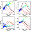 |
Fig. A.1. Line ratio and η-parameter profiles for ESO 544-27 models with varying hzn. The dots show the observed values, colored according to the η-parameter going from blue at low η to green at high η. The size of each dot is relative to the size of the corresponding Voronoi bin. The curves show the model predictions with the color of the curve corresponding with the model hzn, ranging from hzn = 0.6 kpc. (red) to hzn = 1.0 kpc (black) with hzn = 0.1 kpc steps. |
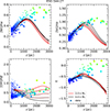 |
Fig. A.2. Line ratio and η-parameter profiles for ESO 544-27 models with varying HOLMES mass. The dots show the observed values, colored according to the η-parameter going from blue at low η to green at high η. The size of each dot is relative to the size of the corresponding Voronoi bin. The curves show the model predictions with the color of the curve corresponding with the model MT, ranging from 0.0 × MT. (black) to 2.0 × MT (red) with 0.5MT steps. |
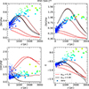 |
Fig. A.3. Line ratio and η-parameter profiles for ESO 544-27 models with varying midplane escape fraction. The dots show the observed values, colored according to the η-parameter going from blue at low η to green at high η. The size of each dot is relative to the size of the corresponding Voronoi bin. The curves show the model predictions with the color of the curve corresponding with the model emp, ranging from emp = 0.2 (red) to emp = 0.8 (black) with emp = 0.15 steps. |
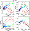 |
Fig. A.4. Line ratio and η-parameter profiles for ESO 544-27 models with varying metallicity. The dots show the observed values, colored according to the η-parameter going from blue at low η to green at high η. The size of each dot is relative to the size of the corresponding Voronoi bin. The curves show the model predictions with the color of the curve corresponding with the model Z0, ranging from Z0 = 8.1 (red) to Z0 = 8.9 (black) with Z0 = 0.2 steps. |
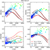 |
Fig. A.5. Line ratio and η-parameter profiles for ESO 544-27 models with varying cloud size. The dots show the observed values, colored according to the η-parameter going from blue at low η to green at high η. The size of each dot is relative to the size of the corresponding Voronoi bin. The curves show the model predictions with the color of the curve corresponding with the model dcloud, ranging from dcloud = 20 pc (red) to dcloud = 180 pc (black) with dcloud = 40 pc steps. |
Appendix B: Images of ESO 443-21, PGC 28308, and PGC 30591
For completeness, we present here some images of the three galaxies that were not part of the sample used in Paper I (ESO 443-21, PGC 28308, and PGC 30591). Figure B.1 shows the η-parameter maps, the Hα equivalent width maps, ionized gas velocity dispersion (σ) maps, and the Veilleux-Osterbrock (VO; Veilleux & Osterbrock 1987) suite of diagnostic diagrams for ESO 443-21 and PGC 30591. For PGC 28308 these were already presented in Fig. 15. Figures 15 and B.1 were derived from the MUSE cubes in the same way as Fig. 14 in Paper I. The S4G 3.6 micron images of ESO 443-21, PGC 28308, and PGC 30591 are shown in Fig. B.2.
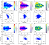 |
Fig. B.1. S4G (Sheth et al. 2010) 3.6 micron images of ESO 443-21, PGC 28308, and PGC 30591. Directions on the sky and 2 kpc scale bars are shown in the images. |
All Tables
All Figures
|
Fig. 1. Schematic of our model. The cyan shaded area indicates the star-forming disk and the large blue stars represent the OB stars within it. The gray shaded areas indicate the eDIG cloud layers, and the filled cyan circles show the eDIG clouds within them. The small purple stars represent the HOLMES between the cloud layers. The colored arrows indicate the source radiation fields of leaking midplane H II regions (SOB(λ); blue), HOLMES (SHOLMES(λ); magenta), and transmitted radiation (St(λ); cyan). Black arrows indicate the cloud diameter (d) and the layer separation (s). |
| In the text | |
|
Fig. 2. Line ratio and η-parameter profiles for ESO 544−27 models with varying U1. The dots show the observed values, colored according to the η-parameter going from blue at low η to green at high η. The size of each dot is relative to the size of the corresponding Voronoi bin. The curves show the model predictions with the color of the curve corresponding with the model log U1, ranging from log U1 = −3.11. (black) to log U1 = −2.91 (red) with log U1 = 0.05 steps. All the models have fV = 0.17. |
| In the text | |
|
Fig. 3. Line ratio and η-parameter profiles for ESO 544−27 models with varying fV. The dots show the observed values, colored according to the η-parameter going from blue at low η to green at high η. The size of each dot is relative to the size of the corresponding Voronoi bin. The curves show the model predictions with the color of the curve corresponding with the model fV, ranging from fV = 0.11. (red) to fV = 0.23 (black) with fV = 0.03 steps. All the models have log U1 = −3.01. |
| In the text | |
|
Fig. 4. Density profile of gas and HOLMES for an ESO 544−27 model. Red dots indicate the cloud layers and blue stars indicate the HOLMES layers. The connecting solid curves plot the densities. For HOLMES, the relative number density defined as the fraction of HOLMES at each layer is plotted. The model parameters are log U1 = −3.01, which is used to determine the density at midplane (see text), and the scale heights of the gas density (hzn = 0.79 kpc), and HOLMES number density (hzT = 0.67 kpc). The gas density of the clouds follows an exponential profile, while the HOLMES number density profile has an exponential component and a constant component with 10% of the mass of the exponential component ((n/N)HOLMES = 2.5 × 10³). |
| In the text | |
|
Fig. 5. [N II]/Hα vertical profiles for our sample galaxies. The blue dots show observed values from Voronoi bins with OB star dominated ionization (η < −0.5). The yellow dots show observed values from Voronoi bins with mixed ionization or ionization dominated by other sources (η > −0.5). The size of each dot is relative to the size of the corresponding Voronoi bin. The solid red curve shows our model for the galaxy in question. The dashed black curve is the same model as the red curve but with HOLMES turned off. The contribution from HOLMES to the ionizing radiation is insignificant for our models when fitting OB star dominated ionization. |
| In the text | |
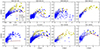 |
Fig. 6. Same as Fig. 5 but for [S II]/Hα. |
| In the text | |
|
Fig. 7. Same as Fig. 5 but for [O I]/Hα. The [O I]/Hα line ratio is poorly fit because [O I] is a collisionally excited line of neutral oxygen, and as such is only produced by partly ionized and neutral gas, while our model emission lines are dominated by fully ionized gas. |
| In the text | |
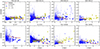 |
Fig. 8. Same as Fig. 5 but for [O III]/Hβ. |
| In the text | |
|
Fig. 9. Contributions of different components to the ionizing radiation for the best fit models. Blue solid lines shows the contribution from midplane OB stars, red dashed line shows the contribution from HOLMES, and the orange dot-dashed line shows the contribution of transmitted radiation. The transition from ionization bounded clouds to density bounded clouds is visible as a steep upturn in the contribution of transmitted radiation. |
| In the text | |
|
Fig. 10. Line ratio profiles for ESO 157−49 model with 2% ΦOB. The dots show the observed values, colored according to the η-parameter going from blue at low η to green at high η. The size of each dot is relative to the size of the corresponding Voronoi bin. The red curve shows the model predictions. This model predicts the [O I]/Hα line ratio well, but fails to predict any of the other line ratios. The log U1 = −4.51 and other parameters are same as in the best fit model. |
| In the text | |
|
Fig. 11. Line ratio and η-parameter profiles for the best fit alternative high-ΦHOLMES ESO 544−27 model (see text). The dots show the observed values, colored according to the η-parameter going from blue at low η to green at high η. The size of each dot is relative to the size of the corresponding Voronoi bin. The solid red curve shows the best fit model including HOLMES (χ2/ν = 39) while the dashed black curve shows the best fit model without HOLMES (χ2/ν = 75). The best fit values for the models including HOLMES are hzn = 1.7 kpc, fV = 0.11, and log U1 = −3.30, while the best fit values for the models without HOLMES are hzn = 1.6 kpc, fV = 0.11, and log U1 = −3.30. The high-ΦHOLMES model reproduces the observed η > −0.5 in the eDIG of ESO 544-27. |
| In the text | |
|
Fig. 12. Line ratio and η-parameter profiles for the best fit PGC 28308 models. The dots show the observed values, colored according to the η-parameter going from blue at low η to green at high η. The size of each dot is relative to the size of the corresponding Voronoi bin. The solid red curve shows the best fit high-ΦHOLMES model (χ2/ν = 156), the dash-dot magenta curve shows the best fit extreme-ΦHOLMES model (χ2/ν = 167), and the dashed black curve shows the best fit model without HOLMES (χ2/ν = 175). The best fit values are hzn = 1.2 kpc, fV = 0.14, and log U1 = −3.10 for the high-ΦHOLMES model, hzn = 1.9 kpc, fV = 0.14, and log U1 = −3.20 for the extreme-ΦHOLMES model, and hzn = 1.1 kpc, fV = 0.14, and log U1 = −3.10 for the model without HOLMES. The reasonable high-ΦHOLMES model fails to reproduce the high η-parameter in the eDIG of PGC 28308, and a model with unrealistically high ΦHOLMES/ΦOB is required to do so. |
| In the text | |
|
Fig. 13. Contributions of the different ionization sources over z for the models with enhanced ΦHOLMES. Top-left panel: contributions of different components to the ionizing radiation for the high-ΦHOLMES ESO 544−27 model. The blue solid line shows the contribution from midplane OB stars, the red solid line shows the contribution from HOLMES, and the cyan and magenta dashed lines show the contribution of transmitted emission from midplane OB stars and HOLMES, respectively. Middle-left panel: same as top-left panel but for the high-ΦHOLMES PGC 28308 model. Bottom-left panel: same as top-left panel but for the extreme-ΦHOLMES PGC 28308 model. Right panel: relative contribution of combined HOLMES radiation and transmitted radiation for all of our models ϕhard = (ΦHOLMES + Φt)/Φ. The thick cyan curve shows ϕhard for the high-ΦHOLMES ESO 544−27 model. The thick dash-dot red curve shows ϕhard for the high-ΦHOLMES PGC 28308 model. The thick solid red curve shows ϕhard for the extreme-ΦHOLMES PGC 28308 model. The dashed curves show ϕhard for the original models. Only models where ϕhard approaches unity are able to produce η > −0.5 in the eDIG. |
| In the text | |
|
Fig. 14. Relative contribution of HOLMES to the model ionizing radiation in eDIG against galaxy sSFR. ESO 544−27 and PGC 28308 are labeled. There is a clear anti-correlation between sSFR and ΦHOLMES/Φ (ρ = −0.79, p = 0.02). |
| In the text | |
|
Fig. 15. Emission-line properties for PGC 28308. (a): η-parameter map. (b): velocity dispersion map. (c): logarithmic EW(Hα) map. The lower limit of the OB-star-dominated ionization (EW(Hα) = 14 Å) is contoured in black. (d)–(f): VO diagrams. The solid line is the Kewley et al. (2001) extreme starburst line, the dashed line in (d) is the Kauffmann et al. (2003) empirical starburst line, and the dash-dot lines in (e) and (f) are the Kewley et al. (2006) Seyfert and low-ionization narrow emission-line region (LINER) demarcation line. The colors in the VO diagrams correspond to the colors in the η-parameter map. While there is no clear biconical morphology in the η-parameter map, the concentration of the eDIG over the center of the galaxy could hint at ionization by outflow driven shocks. Similar figures for ESO 443−21 and PGC 28308 are found in Appendix B. |
| In the text | |
|
Fig. A.1. Line ratio and η-parameter profiles for ESO 544-27 models with varying hzn. The dots show the observed values, colored according to the η-parameter going from blue at low η to green at high η. The size of each dot is relative to the size of the corresponding Voronoi bin. The curves show the model predictions with the color of the curve corresponding with the model hzn, ranging from hzn = 0.6 kpc. (red) to hzn = 1.0 kpc (black) with hzn = 0.1 kpc steps. |
| In the text | |
|
Fig. A.2. Line ratio and η-parameter profiles for ESO 544-27 models with varying HOLMES mass. The dots show the observed values, colored according to the η-parameter going from blue at low η to green at high η. The size of each dot is relative to the size of the corresponding Voronoi bin. The curves show the model predictions with the color of the curve corresponding with the model MT, ranging from 0.0 × MT. (black) to 2.0 × MT (red) with 0.5MT steps. |
| In the text | |
|
Fig. A.3. Line ratio and η-parameter profiles for ESO 544-27 models with varying midplane escape fraction. The dots show the observed values, colored according to the η-parameter going from blue at low η to green at high η. The size of each dot is relative to the size of the corresponding Voronoi bin. The curves show the model predictions with the color of the curve corresponding with the model emp, ranging from emp = 0.2 (red) to emp = 0.8 (black) with emp = 0.15 steps. |
| In the text | |
|
Fig. A.4. Line ratio and η-parameter profiles for ESO 544-27 models with varying metallicity. The dots show the observed values, colored according to the η-parameter going from blue at low η to green at high η. The size of each dot is relative to the size of the corresponding Voronoi bin. The curves show the model predictions with the color of the curve corresponding with the model Z0, ranging from Z0 = 8.1 (red) to Z0 = 8.9 (black) with Z0 = 0.2 steps. |
| In the text | |
|
Fig. A.5. Line ratio and η-parameter profiles for ESO 544-27 models with varying cloud size. The dots show the observed values, colored according to the η-parameter going from blue at low η to green at high η. The size of each dot is relative to the size of the corresponding Voronoi bin. The curves show the model predictions with the color of the curve corresponding with the model dcloud, ranging from dcloud = 20 pc (red) to dcloud = 180 pc (black) with dcloud = 40 pc steps. |
| In the text | |
|
Fig. B.1. S4G (Sheth et al. 2010) 3.6 micron images of ESO 443-21, PGC 28308, and PGC 30591. Directions on the sky and 2 kpc scale bars are shown in the images. |
| In the text | |
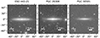 |
Fig. B.2. Same as Fig. 15 but for ESO 443-21 and PGC 30591. |
| In the text | |
Current usage metrics show cumulative count of Article Views (full-text article views including HTML views, PDF and ePub downloads, according to the available data) and Abstracts Views on Vision4Press platform.
Data correspond to usage on the plateform after 2015. The current usage metrics is available 48-96 hours after online publication and is updated daily on week days.
Initial download of the metrics may take a while.