| Issue |
A&A
Volume 583, November 2015
|
|
|---|---|---|
| Article Number | A111 | |
| Number of page(s) | 15 | |
| Section | Cosmology (including clusters of galaxies) | |
| DOI | https://doi.org/10.1051/0004-6361/201425534 | |
| Published online | 02 November 2015 | |
Constraining the intracluster pressure profile from the thermal SZ power spectrum
Argelander-Institut für Astronomie, University of Bonn, Auf dem Hügel 71, 53121 Bonn, Germany
e-mail: This email address is being protected from spambots. You need JavaScript enabled to view it.
; This email address is being protected from spambots. You need JavaScript enabled to view it.
Received: 17 December 2014
Accepted: 19 August 2015
Abstract
The angular power spectrum of the thermal Sunyaev-Zel’dovich (tSZ) effect is highly sensitive to cosmological parameters such as σ8 and Ωm, but its use as a precision cosmological probe is hindered by the astrophysical uncertainties in modeling the gas pressure profile in galaxy groups and clusters. In this paper we assume that the relevant cosmological parameters are accurately known and explore the ability of current and future tSZ power spectrum measurements to constrain the intracluster gas pressure or the evolution of the gas mass fraction, fgas. We use the CMB bandpower measurements from the South Pole Telescope and a Bayesian Markov chain Monte Carlo (MCMC) method to quantify deviations from the standard, universal gas pressure model. We explore analytical model extensions that bring the predictions for the tSZ power into agreement with experimental data. We find that a steeper pressure profile in the cluster outskirts or an evolving fgas have mild-to-severe conflicts with experimental data or simulations. Varying more than one parameter in the pressure model leads to strong degeneracies that cannot be broken with current observational constraints. We use simulated bandpowers from future tSZ survey experiments, in particular a possible 2000 deg2 CCAT survey, to show that future observations can provide almost an order of magnitude better precision on the same model parameters. This will allow us to break the current parameter degeneracies and place simultaneous constraints on the gas pressure profile and its redshift evolution, for example.
Key words: galaxies: clusters: intracluster medium
Member of the International Max Planck Research School (IMPRS) for Astronomy and Astrophysics at the Universities of Bonn and Cologne.
© ESO, 2015
1. Introduction
The scattering imprint of the cosmic microwave background (CMB) radiation from the hot, thermalized electrons in the intracluster medium (ICM) is known as the Sunyaev-Zel’dovich (SZ) effect (Sunyaev & Zel’dovich 1972, 1980), which is playing an increasingly important role in the cosmological and astrophysical research using galaxy clusters. The SZ effect is generally divided into two distinct processes: the kinetic SZ (kSZ) effect describes the anisotropic scattering due to the cluster bulk motion, while the thermal SZ (tSZ) effect describes the inverse Compton scattering of the CMB photons by the thermal distribution of hot electrons in the ICM, which is proportional to the line-of-sight integral of the electron pressure. For the tSZ effect, the energy gain by the CMB photons gives rise to a specific spectral dependence of the tSZ signal, such that below roughly 217 GHz, clusters appear as a decrement and above as an increment in the CMB surface brightness. Because the tSZ surface brightness is independent of the redshift of the scattering source, it provides a powerful means to study the structure and dynamics of the hot intracluster gas throughout cosmic history.
Apart from observing individual clusters, the tSZ effect can also be detected in a statistical sense through the excess power over the primordial CMB anisotropies, coming from all the resolved and unresolved galaxy groups and clusters in a CMB map. Unlike the optical and X-ray observables, the redshift independence of the tSZ signal makes this “confusion noise” a significant source of temperature anisotropies at millimeter/submillimeter wavelengths in the arcmin scale regime, where the primordial CMB anisotropies are damped exponentially. Similar to the cluster number counts, the tSZ anisotropy signal is sensitive to the same set of cosmological parameters because its contribution comes primarily from the hot (≳1 keV), ionized ICM bound to groups and clusters (e.g., Hernández-Monteagudo et al. 2006). The amplitude of the tSZ power spectrum depends roughly on the eighth power of σ8, the rms amplitude of the matter density fluctuations and on the third power of Ωm (Komatsu & Seljak 2002; Trac et al. 2011). However, the tSZ power receives significant contribution from the low mass, high redshifts objects. This seriously hinders its use as a precision cosmological probe, since the thermodynamic properties of these systems are not well constrained from direct observations. Thus, the astrophysical uncertainties in modeling the tSZ power spectrum are too large to place significant constraints on cosmological parameters. Consequently, attention has moved to measuring the higher order statistics of the correlation function, such as the tSZ bispectrum, which arises mostly from massive systems at intermediate redshifts and is therefore less prone to astrophysical systematics (e.g., Rubiño-Martín & Sunyaev 2003; Bhattacharya et al. 2012; Wilson et al. 2012).
As the measurement precision of the cosmological parameters improves from other methods, the use of the tSZ power spectrum in cosmology can be reversed. The tSZ power can then be used as a probe for measuring the distribution and evolution of the intracluster gas, down to low cluster masses and up to high redshifts, where direct observations are difficult. Similar arguments have been presented by several authors (e.g., Shaw et al. 2010; Battaglia et al. 2012a), although a quantitative comparison between the results of analytical cluster pressure models and the observations of the tSZ power spectrum has been lacking. It is also of great interest to know how the future ground-based SZ surveys may constrain the intracluster gas models because their resolutions are better suited to constraining the shape of the tSZ power spectrum.
The amplitude of the tSZ power spectrum was predicted analytically by Komatsu & Seljak (2002), with an expected value of 8−10 μK2 around ℓ = 3000. Later semi-analytic modeling predicted similar values (Sehgal et al. 2010), but experimental results have confirmed these early predictions to be too high. The first conclusive measurement of the combined tSZ+kSZ power spectrum came from the South Pole Telescope (SPT; Lueker et al. 2010). Successive data releases from the SPT and ACT (Atacama Cosmology Telescope) have provided increasingly sensitive and consistent measurements of the tSZ power on arcminute scales (ℓ ~ few × 1000) where the contributions from galaxy groups and clusters are expected to peak (Shirokoff et al. 2011; Dunkley et al. 2011; Reichardt et al. 2012; Sievers et al. 2013; George et al. 2015). Recent results from the Planck spacecraft are also consistent with the SPT value within 2σ (Planck Collaboration XXI 2014), although the Planck resolution cannot resolve the position of the peak of the tSZ power, and is more sensitive on roughly degree angular scales. At these low multipoles, the two-halo correlation term might be important, or the contribution from the warm-hot intergalactic medium (WHIM) might dominate (e.g., Suárez-Velásquez et al. 2013).
In this work we adopt the SPT measurement of CMB bandpowers from Reichardt et al. (2012), which constrained the peak amplitude of the tSZ power spectrum at 150 GHz at 3.65 ± 0.69 μK2. This value is less than half of what was predicted from early semi-analytic cluster models. The source of this discrepancy has been investigated in several works, following analytic and semi-analytic modeling (Shaw et al. 2010; Trac et al. 2011), as well as full hydrodynamical simulations (Battaglia et al. 2012a; McCarthy et al. 2014). These authors identify several physical processes that can produce a lower amplitude of the tSZ power, namely the turbulent bulk motions of the intracluster gas, feedback from supernovae and AGN – plus the redshift evolution of these quantities – that cause cluster properties to deviate from a simple self-similar scaling. The uncertainties in the implementation of various astrophysical processes in these semi-analytical or numerical models remain sufficiently high (~30%, e.g., Shaw et al. 2010), such that cosmological constraints using template models for the tSZ power spectrum are generally not the most competitive.
We aim to make a detailed comparison between analytical models for the intracluster pressure and the latest tSZ power spectrum data, such that errors on the model parameters can be derived directly from observations. This contrasts with earlier analytic or semi-analytic works that were compared against simulation predictions. We set up a Markov chain Monte Carlo (MCMC) based method to explore the range of possible values in the selected pressure model from a set of CMB bandpower measurements, obtaining the full covariance between these parameters. This also allows us to use simulated bandpowers from the future CMB/SZ experiments (e.g., CCAT and SPT-3G) to predict their ability to break the parameter degeneracies and constrain cluster physics.
This paper is organized as follows. In Sect. 2 we describe the “halo model” for computing the tSZ power spectrum, followed-by its measurement technique, and outline our procedure to constrain cluster model parameters from the SPT data. Section 3 summarizes the current knowledge on the cluster pressure structure which will provide the baseline of our work. Section 4 presents our attempts to reconcile the tSZ power spectrum model predictions and available measurements, using altered pressure models. In Sect. 5 we extend our analysis to future SZ cluster survey experiments, and discuss the impact of cosmological parameter uncertainties on the results. We summarize our work in Sect. 6 and present conclusions. Throughout this work we assume a ΛCDM cosmology with h = 0.71, Ωm = 0.264, Ωb = 0.044, ΩΛ = 0.736, ns = 0.96, and σ8 = 0.81 (Komatsu et al. 2011).
2. Method
In this section we describe the halo formalism for computing the tSZ power spectrum, and the observation and modeling of the microwave sky that we use in a Bayesian MCMC formalism to constrain cluster pressure model parameters.
2.1. Analytical estimate of the tSZ power spectrum
2.1.1. From the halo model to the power spectrum
The tSZ power spectrum consists of one-halo and two-halo contributions. The one-halo term results from the Comptonization profile of individual halos in a Poisson distributed population, while the two-halo term accounts for the two-point correlation function between individual halos. For intermediate to small angular scales (ℓ ≳ 1000), which correspond to the angular size of individual galaxy clusters (θ ≲ 10′), Komatsu & Kitayama (1999) showed that the one-halo Poisson term is by far the dominant contribution. Following their prescription, the analytical expression of the tSZ power reduces to the formula 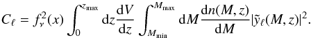 (1)Here dV/ dz is the co-moving volume of the Universe per unit redshift z,
  is the spherical harmonics decomposition of the sky-projected Compton y-parameter, dn(M,z)/dM is the dark matter halo mass function, fν(x) is the spectral function of the tSZ effect given by
 ![Mathematical equation: \begin{equation} f_{\nu}(x)=\bigg(x\frac{e^{x}+1}{e^{x}-1}-4\bigg)[1+\delta_{\textrm{SZ}}(x)],\label{spectral_function} \end{equation}](/articles/aa/full_html/2015/11/aa25534-14/aa25534-14-eq30.png) (2)where x ≡ 2πħν/kBTCMB, and δSZ(x) is the relativistic correction to the frequency dependence. The reduced Planck constant is ħ, kB is the Boltzmann constant, and TCMB is the CMB temperature. We do not include relativistic corrections to fν(x) as they have a negligible effect at the temperatures of groups and low-mass clusters which dominate the tSZ power spectrum.
(2)where x ≡ 2πħν/kBTCMB, and δSZ(x) is the relativistic correction to the frequency dependence. The reduced Planck constant is ħ, kB is the Boltzmann constant, and TCMB is the CMB temperature. We do not include relativistic corrections to fν(x) as they have a negligible effect at the temperatures of groups and low-mass clusters which dominate the tSZ power spectrum.
The integral in Eq. (1) is insensitive to z ≳ 4 due to the absence of sufficiently massive halos. In our calculations, we thus set the upper redshift boundary to zmax = 6. Similarly, to cover a maximum critical mass range for galaxy groups and clusters, we set Mmin = 1012h-1M⊙ and Mmax = 1016h-1M⊙. We use the mass function obtained by Tinker et al. (2008).
From Komatsu & Seljak (2002), the spherical harmonics contribution of a given Compton y-parameter profile on angular scale ℓ is given by 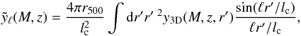 (3)where r′ ≡ r/r500 is a scaled, non-dimensional radius, lc ≡ DA/r500 is the corresponding angular wavenumber, and y3D is the 3D radial profile of the Compton y-parameter. This last parameter is given by a thermal gas pressure profile, Pgas, through
 ![Mathematical equation: \begin{eqnarray} y_{\textrm{3D}}(M,z,r^{\prime}) &\equiv& \frac{\sigma_{T}}{m_{\rm e}c^{2}}P_{\rm e}(M,z,r^{\prime})=\frac{\sigma_{\textrm{T}}}{m_{\rm e}c^{2}}\bigg(\frac{2+2X}{3+5X}\bigg)P_{\textrm{gas}}(M,z,r^{\prime})\nonumber \\ &=& 1.04\times 10^{4}~\textrm{Mpc}^{-1}\bigg[\frac{P_{\textrm{gas}}(M,z,r^{\prime})}{50~\textrm{eV cm}^{-3}}\bigg], \label{y_3D} \end{eqnarray}](/articles/aa/full_html/2015/11/aa25534-14/aa25534-14-eq47.png) (4)where Pe is an electron-pressure profile, X = 0.76 is the Hydrogen mass fraction, σT is the Thomson cross-section, me is the electron mass, and c is the speed of light.
(4)where Pe is an electron-pressure profile, X = 0.76 is the Hydrogen mass fraction, σT is the Thomson cross-section, me is the electron mass, and c is the speed of light.
2.1.2. Effect of the intrinsic pressure scatter
Despite the tight correlation between the tSZ signal and cluster mass, several works have shown that the dispersion of individual cluster pressure profiles Pe(r′) at a given mass is far from negligible (~30% according to Planck Collaboration XXXI 2013; and Sayers et al. 2013). So far the contribution of this scatter has not been considered in analytical treatments of the tSZ power spectrum. Modeling this effect would indeed require a detailed knowledge of the diversity of cluster Comptonization morphologies. Observationally this is not yet well-constrained as tSZ experiments still aim at improving our estimate of the average cluster pressure profiles.
In our modeling of the tSZ power, we try to capture the bulk contribution of the intrinsic scatter. To do so, we make the assumption that the dispersion in the pressure structure can be encapsulated in a simple scatter on the normalization of the pressure profile, leaving the shape unchanged. In this case, marginalizing over the distribution of profile normalization results in a straightforward scaling of the tSZ power spectrum amplitude as follows: 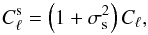 (5)where σs is the intrinsic scatter on the Pe(r′) normalization. With this approximation, the 30% intrinsic scatter on the pressure amplitude increases the tSZ power amplitude by roughly 10%. We include this additional contribution in all subsequent results. More details on the adopted pressure profile and the measurement of intrinsic scatter are given in Sect. 3.
2.2. Microwave sky model
Our analysis relies on the microwave extragalactic power spectra published by Reichardt et al. (2012, hereafter R12) for three different frequency bands. Those observations were extracted from 800 deg2 maps obtained within the SPT survey and cover angular scales of 2000 <ℓ< 10000.
Such observations are a combination of signals from primary CMB anisotropy, foregrounds, and secondary SZ anisotropies. The power spectrum from each of these components has different frequency dependence, so detailed multifrequency observations can in principle distinguish their relative contributions in the maps (see e.g., Planck Collaboration XII 2014). Unfortunately, three frequencies are not sufficient to perform this kind of analysis. Instead, we have to rely on a model for the microwave sky power, calibrated using external information wherever possible. The problem then reduces to a decomposition of the observed signal into a set of templates, for which mostly the normalization has to be quantified.
In this purpose, we use the same model as in R12 where the total microwave sky power,  , breaks down into the following components:
  (6)Here,
  is the lensed primary CMB anisotropy power at multipole ℓ. On scales ℓ> 3000, is strongly damped, and other components start to dominate. The population of dusty star-forming galaxies (DSFGs) have a significant microwave emission (specially at high frequencies), which contributes with Poisson (
 ) and clustered (
 ) power components. Likewise, mainly at low frequencies, the population of radio sources contributes prominently with a Poisson term,
  . A small contribution from the Galactic cirrus emission,
  , is also taken into account. Finally, the power of the tSZ and kSZ signals are given by
  and
and  , respectively.
Our work can therefore be considered as an astrophysical extension of the analysis presented by R12, where we allow for more freedom in the tSZ power spectrum by tieing it to a range of empirical models of the ICM. The other components of our baseline model are treated as nuisance parameters and described in detail in Appendix A.
2.3. Parameter estimation
The SPT measurements as described in R12 comprise three auto-spectra (95 × 95, 150 × 150, 220 × 220 GHz), and three cross-spectra (95 × 150, 95 × 220, 150 × 220 GHz), in 15 spectral bands bℓ, each covering a narrow range in ℓ. In our work, we seek to match the parameters of intracluster pressure models with those observations. This is achieved by minimization of the χ2 statistic, 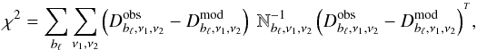 (7)where
  and
and  are respectively the observed and modeled powers in band bℓ, and
  is the bandpower noise covariance matrix (obtained from R12), for the cross-spectra at frequencies ν1 and ν2.
The modeled bandpowers are estimated from the full-resolution power spectra of Eq. (6) and the band window functions wℓ,bℓ (also obtained from R12) as: 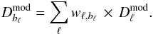 (8)The best fit parameters and their errors are obtained by sampling the likelihood function over the whole parameter space using a MCMC Metropolis algorithm.
In order to validate our modeling of the SPT data and our fitting procedure, we first replaced our analytical tSZ model with the template provided by Shaw et al. (2010)− as done in R12− and jointly fitted the amplitudes of the tSZ template ( ), Poisson (
 ) and clustered (
 ) CIB components, fixing all other parameters to the R12 values. The results of this three-parameter samplings are displayed in Table 1 and Fig. 1, and are in agreement with R12. As expected, the errors in our result are smaller, since we held fixed the cosmological parameters and several of the foreground components. However, the difference is not large, reflecting the fact that the three fitted components are the leading contributors to the microwave background anisotropies on the considered wavelengths and angular scales.
In the following, we always fit the amplitudes of the Poisson and clustered CIB components together with our cluster pressure model parameters. Given the small impact they have on the final measurements, the additional components (lensed CMB, kSZ effect, radio and Galactic cirrus) are kept fixed for simplicity, and so are the cosmological parameters. The cosmological constraint is discussed in more detail in Sect. 5.3.
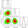 |
Fig. 1 2D likelihoods for the power spectra amplitudes at ℓ = 3000 using our MCMC algorithm, compared to the results from R12. The plot shows the tSZ power spectrum ( |
3. Pressure model
In this section we introduce briefly the self-similar theory that describes the properties of galaxy groups and clusters. We also explain in detail the latest measurements of the pressure profile in galaxy clusters, and show the inconsistency between the SPT measurements and the theoretical predictions for the tSZ bandpowers based on such pressure profiles.
3.1. Self-similar models
In a hierarchical structure formation scenario on a cold dark matter (CDM) cosmology, groups and clusters are the end products of gravitational collapse of a small population of highly over-dense regions in the early Universe. The term “self-similar” points to the scale-free nature of gravitational collapse in such a Universe (Kaiser 1986). This implies that if clusters were strictly self-similar, we would expect the same evolution of their global properties on any scale and time. In the context of self-similar evolution, the redshift dependence of cluster observables can be expressed as a combination of different powers of E(z) and Δ(z), where 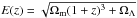 is the Hubble ratio in flat ΛCDM Universe, and Δ(z) is the density ratio between the mean (or critical) density of the Universe at redshift z and that inside a fiducial radius of the cluster.
Furthermore, a self-similar formation model implies that gravitational collapse is the only source of energy input into the ICM. Since we assume cluster formation process is governed by gravity alone, we can derive simple scaling relations for the global observables properties as a function of cluster mass. These relations have been extensively studied in the literature (see Böhringer et al. 2012, and references therein). Particularly in the nearby Universe, they have been studied and determined with high precision. In the following section we describe the current state of knowledge on the self-similar redshift evolution and mass scaling of the ICM pressure profile.
3.2. The “universal” pressure profile
One of the most successful application of the self-similar model is the dark matter halo mass profile measured from N-body simulations by Navarro, Frenk, & White (1995), known as the NFW profile. Following this model a more generalized version was proposed by Nagai et al. (2007) to describe the gas distribution in galaxy clusters, which contains additional shape parameters besides the normalization and the scale radius (generalized NFW, or GNFW profile). Arnaud et al. (2010, hereafter A10) measured these parameters for the GNFW model, as well as the mass scaling of the overall normalization, combining X-ray data and numerical simulations. This was the first demonstration of a scale-free, universal shape of the cluster pressure profile with a mass scaling very close to self-similar. The parametrization of the GNFW pressure model found by A10 is now commonly known as the “universal” pressure profile, and forms the basis of our analytical modeling.
A10 measured the GNFW profile parameters from a sample of 33 local clusters (z< 0.2), selected from the REFLEX catalogue and observed with XMM-Newton. The sample covers a mass range 7 × 10¹³ ≲ M500h/M⊙ ≲ 6 × 10¹⁴, where M500 is the mass enclosed within r500, in which the mean density is 500 times the critical density of the Universe. The pressure profile is given by ![Mathematical equation: \begin{equation} P_{\textrm{e}}(r^{\prime})\!=\!1.65\bigg(\frac{h}{0.7}\bigg)^{2}\!\textrm{eV cm}^{-3}~E^{\frac{8}{3}}(z)\bigg[\frac{M_{500}}{3\!\times\!10^{14}(0.7/h)~{M}_{\odot }}\bigg]^{\frac{2}{3}+\alpha_{\rm p}} \! p(r^{\prime}). \label{A_pressure} \end{equation}](/articles/aa/full_html/2015/11/aa25534-14/aa25534-14-eq110.png) (9)The function p(r′) describes the scale-invariant shape of the pressure profile,
(9)The function p(r′) describes the scale-invariant shape of the pressure profile, ![Mathematical equation: \begin{equation} p(r^{\prime})\equiv \frac{P_{0}(0.7/h)^\frac{3}{2}}{(c_{500}r^{\prime})^{\gamma}[1+(c_{500}r^{\prime})^{\alpha}]^{(\beta-\gamma)/\alpha}}, \label{gnfw_profile} \end{equation}](/articles/aa/full_html/2015/11/aa25534-14/aa25534-14-eq112.png) (10)where P0 = 8.403, c500 = 1.177 is a gas concentration parameter, the parameter γ = 0.3081 represents the central slope (r′ ≪ 1), α = 1.051 is the intermediate slope (r′ ~ 1), and β = 5.4905 is the outer slope (r′ ≫ 1) of the pressure profile. The A10 profile was constrained from X-ray observations out to radii r ~ r500. Beyond this radius, an extrapolation was made to fit the results from numerical simulations of clusters (Borgani et al. 2004; Nagai et al. 2007; Piffaretti & Valdarnini 2008). A small deviation from the self-similar scaling with cluster mass is given by αp = 0.12. We incorporate this additional mass dependence in all our calculations, which has a small effect on the amplitude of the tSZ power (~9% at ℓ = 3000). We ignore the extra smaller shape-dependent term of the mass scaling, described by the
(10)where P0 = 8.403, c500 = 1.177 is a gas concentration parameter, the parameter γ = 0.3081 represents the central slope (r′ ≪ 1), α = 1.051 is the intermediate slope (r′ ~ 1), and β = 5.4905 is the outer slope (r′ ≫ 1) of the pressure profile. The A10 profile was constrained from X-ray observations out to radii r ~ r500. Beyond this radius, an extrapolation was made to fit the results from numerical simulations of clusters (Borgani et al. 2004; Nagai et al. 2007; Piffaretti & Valdarnini 2008). A small deviation from the self-similar scaling with cluster mass is given by αp = 0.12. We incorporate this additional mass dependence in all our calculations, which has a small effect on the amplitude of the tSZ power (~9% at ℓ = 3000). We ignore the extra smaller shape-dependent term of the mass scaling, described by the  term (see Eq. (10) in A10), because it has a negligible contribution (~2% at ℓ = 3000). Finally, the derived average A10 pressure profile has a dispersion around it, which is less than 30% beyond the core (r> 0.2r500), and increases towards the center. This deviation around the mean is mainly due to the dynamical state of the clusters. Following 2.1.2 we assume this scatter only affects the pressure shape normalization (P0), and incorporate its contribution into our power spectrum calculations accordingly.
The nearly self-similar mass scaling of the universal pressure profile has been verified down to the low mass end (galaxy groups) in the local Universe. Sun et al. (2011) extended the measurements of A10 to lower masses, from a study of 43 galaxy groups at z = 0.01−0.12, within a mass range of roughly M500 = 1013−1014hM⊙. All the ICM properties of these groups were derived at least out to r2500 from observations made with Chandra, and 23 galaxy groups have in addition masses measured up to ~r500. As with the original data set used by A10, the X-ray comparison by Sun et al. (2011) does not reveal the state of the gas pressure in groups at higher redshift, or at radii beyond r500. Nevertheless, this rules out the possibility of a highly non-self-similar mass scaling for the ICM pressure, at least in the low redshifts, in a mass range spanning nearly two decades. Recent results by McDonald et al. (2014), using X-ray follow-up observation of SZ selected clusters, also confirm the validity of the universal pressure profile in a wide redshift range, down to a mass limit M500 ~ 3 × 10¹⁴M⊙. These are strong constraints while finding modifications for the universal pressure model to match the tSZ power spectrum observation.
Direct tSZ observations of individual clusters have now verified the validity of the universal pressure model at the high mass end, even though measurement errors remain high. In contrast to the X-ray measurement of the GNFW profile, tSZ observations are more sensitive to the cluster outskirts (r>r500). Planck Collaboration XXXI (2013) measured the pressure profile of a sample of high mass and low redshift galaxy clusters. Their mean profile shows a slightly lower pressure in the inner parts when compared with the A10 profile, although there are strong degeneracies between the derived model parameters. It is possible that the lower pressure in the core region detected by Planck is a consequence of detecting more morphologically disturbed clusters than other samples. Outside the core region the Planck-derived pressure profile show good agreement with the extrapolated A10 pressure model, out to a radius ~3r500. It should be noted that the poor angular resolution of Planck restricts its sensitivity for the pressure profile shape measurement mostly to a handful of nearby, massive clusters detected with high signal-to-noise ratio.
A higher-resolution tSZ observation of individual cluster pressure profiles became available from the Bolocam experiment (Sayers et al. 2013), which has 1 arcminute resolution at 150 GHz. The Bolocam team observed 45 massive galaxy clusters, with a median mass of M500 = 9 × 10¹⁴M⊙, and spanning a large range in redshift: 0.15 <z< 0.89. They fitted a GNFW profile between 0.07r500 and 3.5r500. Despite the strong covariance between the model parameters, the overall shape is fairly well constrained. The mean profile shows good agreement with the A10 model, although there is an indication of a shallower pressure outer slope (r ≳ r500). Furthermore, both Planck and Bolocam teams have measured the intrinsic scatter for the pressure profile in their samples, finding it to be roughly 30% as was also noted by A10. In the absence of more accurate measurements, we use σs = 0.3 (see Eq. (5)) as a fiducial value in the rest of the paper.
An important point to note here is that neither the Planck not the Bolocam analysis is based on a representative sample of galaxy clusters. Therefore, although these two data sets serve to constrain the alterations to the A10 pressure model in Sect. 4, none can yet be considered compelling.
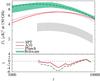 |
Fig. 2 Discrepancy between the semi-analytic model predictions for the tSZ power and the SPT measurements. The red solid line is the tSZ power spectrum given by the A10 pressure profile (Eq. (9)). The shaded gray region represent the 1σ constraints from the SPT, which is restricted by the shape of the Shaw model (see text for details). The purple dot-dashed line gives the result for the mean GNFW profile as measured by Planck (Planck Collaboration XXXI 2013). The green band marks the corresponding Bolocam measurement (Sayers et al. 2013) with the 68% confidence interval on their model fit parameters. The bottom panel shows the value of χ at each point for these models with respect to the SPT bandpower measurements, in units of the measurement errors in each ℓ-band. |
3.3. Discrepancy between theoretical prediction and observation of the SZ power spectrum
The discrepancy between the theoretical model predictions for the tSZ power spectrum and its experimental measurement were shown early on, following pure analytical modeling (Komatsu & Seljak 2002; Bode et al. 2009) and simulations (Sehgal et al. 2010). The tSZ power based on the A10 universal pressure model is not the exception, as is shown in Fig. 2. The red solid curve is the prediction based on the A10 model, using Eqs. (1) and (9), which has a factor of ~2 higher amplitude than the SPT measurement (marked by the gray-shaded region). Similar results were also shown by Efstathiou & Migliaccio (2012).
We point up that despite its high sensitivity, the SPT data is unable to constrain simultaneously both the amplitude and shape of the tSZ power spectrum. For this reason R12 used the Shaw et al. (2010) tSZ template to quote the amplitude at ℓ = 3000, which is 3.65 ± 0.69 μK2. In Fig. 2 and subsequent plots, we show the SPT 68% confidence region derived from the Shaw et al. (2010) model in gray bands, to provide a visual comparison with our best fit results. The plots are in terms of 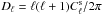 with units of [μK]2 at 150 GHz. For quantifying the goodness of fit between a model prediction and the SPT data, we compute the probability to exceed (PTE, or the p-value) for the model using the actual CMB bandpower measurements from SPT, and not with the Shaw et al. (2010) model template. The PTE for the A10 model prediction is 0.0006, suggesting a very poor fit.
It is now possible to check the compatibility of the Planck and Bolocam measurements of the pressure profile with the SPT result following the procedure outlined in Sect. 2. These are shown in Fig. 2 with the dotted and dashed lines, respectively. The prediction based on the mean Planck profile is very similar to the A10 model, whereas the mean Bolocam profile predicts higher amplitude for the tSZ power and returns further lower PTE value. This is primarily because of the shallower outer slope of the pressure profile as reported in the Bolocam paper, giving excess power al ℓ ≲ 3000. We take note of the fact that making a comparison with only the mean pressure profile, using the maximum likelihood values of the GNFW model parameters, is not correct since there is a large covariance between these parameters which will produce a range of equally likely pressure profiles. The Planck parameter covariance is not published, but we obtained the parameter chains for the GNFW model fit for Bolocam (J. Sayers, priv. comm.), which allow us to draw a 68% credibility region of the tSZ power spectrum based on the Bolocam result. This is shown by the green shaded region in Fig. 2, which is small compared to the roughly 5 μK2 difference between the predicted power and the SPT measured value. Based on similar parameter errors on the GNFW model fit by Planck Collaboration XXXI (2013), it can be assumed that the measured errors on the mean Planck profile cannot explain the mismatch with data either.
It can be argued that the source of the discrepancy between the predicted amplitude of the tSZ power spectrum and its measurement comes from the assumed cosmological model. The tSZ power spectrum relies on the correct modeling of the halo mass function, but it has been proven that the halo mass function is known to an accuracy of about 5% (Tinker et al. 2008; Bhattacharya et al. 2011). However, the values of the key cosmological parameters differ significantly between the measurements made by different probes, like WMAP and Planck , which will result in large systematic changes in the tSZ power spectrum. In Sect. 5.3 we address this issue in more detail, and show if we ignore the large systematic difference between the WMAP and Planck cosmology, then the measurement uncertainties in any of the adopted set of parameters is not an issue. Moreover, use of the Planck cosmology increases the predicted tSZ power amplitude by roughly factor 2, thereby making the tension between theory and observation more severe. Since we observe a reduced amplitude of the tSZ power, the most likely explanation for that lower amplitude must be astrophysical, and our use of WMAP cosmology amounts to a more conservative modification of the ICM pressure distribution to match theory and observation.
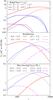 |
Fig. 3 Contribution of the tSZ power spectrum in different cluster radial, mass and redshift bins. The plot is in terms of |

3.4. Radial, mass and redshift contribution to the power spectrum
We split the tSZ power into mass, redshift and radial bins to identify where the main contributions to the tSZ power come from. The results in this section are similar to those already presented in Komatsu & Seljak (2002), Battaglia et al. (2012b) and McCarthy et al. (2014), although we use the universal pressure model of A10 for our analysis.
First, we radially truncate the pressure profile to investigate which regions of the galaxy clusters contribute more to the total tSZ power spectrum. The differential contributions from three radial bins are shown in Fig. 3 (top panel). Earlier works have shown the results for radial contributions in cumulative plots, which automatically include the cross-correlation of the tSZ power between different bins. We make a differential plot for ease of comparison and take the cross-correlation terms into account. When considering all clusters at all redshifts, most of the power (~85%) on small angular scales (ℓ> 3000) comes from r<r500, since bulk of the cluster tSZ signal comes from this central region. Outskirts of galaxy clusters play an important role at lower ℓ. The tSZ power increases by ~50% at ℓ = 500 when the upper limit of the radial integration is increased to 2r500. Thereafter, the tSZ amplitude does not vary much if the integration limit is extended to radii r> 4r500. If we only consider clusters at high redshifts (z> 0.5), the power contribution from the outskirts will be roughly equal to that coming from the inner region for ℓ ≲ 2000 (dashed-lines in the upper panel of Fig. 3).
In a similar way, we calculate the tSZ power spectrum in mass and redshift bins, which are shown in the middle and bottom panels of Fig. 3, respectively. On large angular scales (ℓ< 2000) the largest contribution to the tSZ power comes from high mass (14 < log [M500h/M⊙] < 14.5) and low redshift objects (z< 0.2). Above ℓ ~ 3000, the tSZ power is dominated by low mass (13.5 < log [M500h/M⊙] < 14) and high redshift (z> 0.5) galaxy groups/clusters. The very massive objects (log [M500h/M⊙] > 14.5) have a negligible contribution on small angular scales. Therefore the clusters that are currently constrained from direct tSZ observation by Planck and Bolocam are not representative in terms of the measurement of the tSZ power spectrum. Objects with very low mass, or redshift z> 1 dominate the tSZ power only at multipoles larger than ℓ ~ 15000, assuming the extrapolation of the A10 pressure model is correct in such extreme cases.
From the illustrations above it can be seen that the tSZ power near the angular scales of its expected peak is dominated by contributions from the low mass clusters or groups at intermediate redshifts, for which there are little observational constraints on their ICM properties. Thus, using the fiducial values for the A10 pressure model on high redshift galaxy groups and clusters could be the source of the over-estimation of the tSZ power. Likewise, the A10 pressure profile beyond r500 was constrained from hydrodynamical simulations, which could also be overestimating the thermal pressure component in the outskirts, giving more tSZ power. Thus, two obvious choices for modifying the A10 pressure profile would be i) decreasing the pressure amplitude with redshift that offsets the self-similar evolution; or ii) decreasing the thermal pressure support in the outskirts.
The mass dependence of the pressure normalization (or the outer pressure slope), as discussed in Sect. 4, are generally better constrained from observation (or simulations) and are not the main focus of the current paper.
3.5. Effect of cluster morphology
Before proceeding to modify the universal pressure profile, it is natural to ask whether an over-abundance of merging systems at high redshifts can be responsible for the lower measured tSZ power. This follows from the result of A10 who found, with high significance based on X-ray data, that disturbed clusters have lower pressure near the core region compared to the mean. In the standard ΛCDM scenario the number of mergers within a time interval is a slowly increasing function of halo redshift and mass (e.g., Fakhouri et al. 2010), and there is some evidence of this increased merger fraction from X-ray selected clusters (Maughan et al. 2012; Mann & Ebeling 2012). The resulting change in the cool-core (CC) to non cool-core (NCC) cluster ratio with redshift might be causing the lower amplitude of the tSZ power spectrum in the SPT data.
A10 divided their cluster sample into CC and NCC clusters and provided parametric fits for the respective populations (see Appendix C of A10). The CC clusters have more peaked profile at the center, the region that produces bulk of the emissivity in X-rays. However, from Fig. 4 we can conclude that the core region (r< 0.2r500) contributes a negligible fraction of the tSZ power on scales larger than ~1 arcmin: the contribution is only 5% at ℓ = 3000, and rises up to nearly 17% at ℓ = 10 000. A10 found the pressure profiles of the CC and NCC cluster samples nearly self-similar in the intermediate (r ~ r500) to outer regions, and currently there are no direct evidence for a systematic difference between the CC and NCC cluster pressure distribution from tSZ data. Given that restriction, the CC and NCC clusters produce roughly the same result for tSZ power (Fig. 4). We thus conclude that an increased occurrence of NCC clusters at high-z cannot be the explanation of the low measured value of the tSZ power, if those NCC clusters follow the same mass and redshift scaling as given for the universal pressure profile by A10.
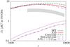 |
Fig. 4 Predictions for the tSZ power spectrum for cluster morphological evolution. The red-solid line is given by the mean A10 pressure profile, the green-dashed line for cool-core clusters, and the blue short-dashed line for non-cool clusters. The purple dot-dashed line shows the relative contribution from the core regions of galaxy clusters (r< 0.2r500) to the total tSZ power, and the dotted line above it factors in an additional scatter contribution (40%) for the core region. This plot shows that, unlike the X-ray luminosity, the core region contributes very little to the tSZ anisotropy power. |
4. Results
This section presents our main results, following various attempts at modifying the universal pressure model. We group these model changes according to their deviations from a simple self-similar scaling.
4.1. Modification following strictly self-similar evolution
In the classical self-similar scenario of cluster evolution, the baryon distribution will have the same shape and amplitude once they are scaled to the cluster mass and redshift with the standard scaling powers (e.g., Böhringer et al. 2012). In context of the A10 pressure profile, this means that clusters at all mass and redshift will have the same set of amplitude and shape parameters: { P0,c500,α,β,γ }, and the total pressure amplitude will scale with redshift as E(z)8/3. In a first attempt to keep the redshift evolution unchanged, we try to find a suitable set of shape parameters that will remove the tension between the model predictions and SPT data.
4.1.1. Constraints on the outer slope of the pressure profile
As mentioned previously, the “universal” pressure profile was constrained from X-ray observations out to radii r ~ r500, and extrapolated beyond r500 to match hydrodynamical simulation results. The outer slope parameter is denoted by β, whose value is fixed at β = 5.49 in the A10 paper. A significant amount of the tSZ signal comes from r>r500, more than 50% if we neglect the few nearby, high-mass clusters (that are generally resolved in deep tSZ surveys), therefore the impact of β on the tSZ power amplitude is pivotal. A higher value of β would imply less thermal pressure. Physical reason for lower thermal pressure can be additional pressure support from gas bulk motions, usually triggered by infalling or merging sub-halos. Recent results from numerical simulations (Nagai et al. 2007; Lau et al. 2009; Nelson et al. 2014) as well as analytical modeling (Shi & Komatsu 2014) have shown that this non-thermal pressure contribution is small in the inner regions, but rapidly increases with radius. We therefore concentrate on modifying β, given the least amount of observational constraint on its value, while keeping the redshift evolution of the pressure amplitude at E(z)8/3 as in Eq. (9).
The best fit value obtained from our MCMC sampling is β = 6.35 ± 0.19, together with the CIB contribution terms 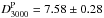 and
and  . The resulting PTE = 0.80 suggests a good fit to the CMB bandpower data. This value of β is considerably higher than the one assumed by A10 (β = 5.49), implying a much lower thermal pressure support in the outskirts. This new value of β has very little effect on the inner pressure profile (<1% at r ≪ r500), but reduces the pressure amplitude by ~40% at r500. The effect is significant on the power spectrum after projection, especially on large scales, where the new tSZ power amplitude is lowered by ~50% compared to the A10 values (Fig. 5, blue dashed line). Furthermore, the peak of the tSZ power spectrum is shifted to smaller angular scales, near ℓ ~ 4500. We note that the shape of the tSZ power spectrum differs strongly compared to the Shaw et al. (2010) template (gray band), but the new shape provides acceptable fit to the SPT data together with the above CIB power amplitudes.
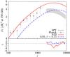 |
Fig. 5 Predictions for the tSZ power spectrum for self-similar evolution. The red solid line is the tSZ power spectrum given by the A10 pressure profile (Eq. (9)). The shaded gray region represent the 1σ constraints from the SPT based on the Shaw et al. (2010) template (see text for details). The blue dashed line represents the GNFW model with our best fit outer slope (β = 6.35), which provides good fit to the actual SPT data, as shown by the χ plot in the bottom panel. The black data points are the marginalized bandpowers of the Planck tSZ power spectrum, taken from Planck Collaboration XXI (2014). |
4.1.2. Possible tension with Planck and Bolocam results
The marginalized value of the outer pressure profile slope, β = 6.35 ± 0.19 with 68% confidence, is higher than the mean values obtained from direct cluster SZ profile measurement by Bolocam and Planck experiments. However, in a GNFW model fit the value of β generally highly degenerates with other parameters, in particular it anti-correlates with the scale radius (or equivalently, c500), as shown by Planck Collaboration XXXI (2013). Therefore we must compare our best fit values with the marginalized errors on β from other experiments. This is shown in Fig. 6, where we plot the normalized likelihood distributions for the outer slope parameter β from Planck and Bolocam fits. As can be seen, there is significant tension for such a steep value of outer slope with Bolocam data, whereas it is consistent with the Planck measurement. A possible cause can be that the Bolocam team fixes the gas concentration parameter c500, which restricts their likelihood range of β, even though both our modeling and the Bolocam work by Sayers et al. (2013) use the same fixed value c500 = 1.18 from the A10 model. The sensitivity of the Planck measurement to the slope parameters is possibly lower due to its large beam, except for a few nearby clusters.
A general consequence of having a steeper outer slope is that it will inevitably reduce the tSZ power at low ℓ values (ℓ< 1000), as seen in Sect. 4.1.1. This then leads to some tension with the tSZ power measurements based on Planck data (Planck Collaboration XXI 2014), which we show in Fig. 5. The Planck marginalized bandpower values are taken directly from the Planck collaboration paper. Without a knowledge of the covariance we cannot compute the χ2 or the PTE value of our model from Planck data, but a clear tension can be seen from the figure.
4.2. Weakly self-similar: changing pressure normalization with redshift or mass
It is possible to imagine scenarios where the amplitude of the pressure distribution in galaxy clusters deviate from a strictly self-similar evolution, i.e., not scaling as  or/and P(r) ∝ E(z)8/3. In fact A10 already show that the mass scaling of the pressure profile is not strictly self-similar, there is an additional factor, αP = 0.12, in the mass-scaling power (see Eq. (9)). The reason behind this deviation from self-similarity is the empirical calibration of the A10 pressure profile against the measured YX−M500 scaling of Arnaud et al. (2007), which was based on a subset of REXCESS clusters at low redshifts. Therefore, while the small deviation in the mass exponent in Eq. (9) is well-measured in the local Universe, its redshift dependence remains largely unexplored.
In this section we explore scenarios where the redshift evolution of the pressure amplitude deviates from the E(z)8/3 scaling, while keeping the shape (Eq. (10)) constant. Physical motivation for such redshift dependence can be found from the observed scaling of the LX−TX scaling relation (e.g., Reichert et al. 2011), possibly relating to a gas mass fraction, fgas, evolution in groups and clusters which we discuss subsequently. As an extension to this model, we consider cases where the redshift evolution depends also on mass, in line with the observed difference in the mass dependence of fgas in groups and clusters.
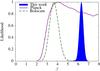 |
Fig. 6 1D likelihood curves for outer slope parameter β. The purple solid line shows the constraints from Planck . Results from Bolocam are shown by the green dashed line. The blue-filled curve represents our best fit constraint on β. |
4.2.1. Departure from self-similar redshift evolution
As discussed in Sect. 3.1, in the self-similar model the redshift evolution of the global properties of galaxy clusters is described by a simple power law of the E(z) parameter. However, non-gravitational processes, like cooling and feedback, can alter the expected redshift evolution parametrization (e.g., Voit 2005). Such possible deviations from self-similarity can be considered through a (1 + z) term lacking a better understanding of their origin. Recent semi-analytical works (Shaw et al. 2010; Battaglia et al. 2012a) have also used a power-law dependence of (1 + z) for modeling the non-thermal pressure evolution.
Following the above argument, and keeping the functional form of the A10 pressure profile unchanged at low redshifts, we introduce an additional (1 + z) dependence of the form  (11)The parameter αz signifies the departure from the self-similar evolution, and we constrain its value by comparing with the SPT measurements (R12) through our MCMC method. The best fit value is αz = −0.73 ± 0.16,
  , and
, and  , with a PTE of 0.78. The overall effect of such non self-similar evolution is to lower the amplitude of the tSZ power spectrum (purple-dotted line in Fig. 7), since as the negative value for αz implies, the pressure amplitude in groups/clusters decreases with increasing redshift. The modified shape of the tSZ power spectrum is in good agreement with the Shaw et al. template (Fig. 7).
From a cosmological point of view, a power-law dependence of E(z) is a more attractive parametrization for the non-self-similar evolution. Efstathiou & Migliaccio (2012) have proposed such a model by introducing the parameter ϵ into the E(z) power for the pressure scaling:  (12)As before, we can constrain the value of ϵ by comparing with the SPT measurements. We find values of ϵ = 1.17 ± 0.27,
  , and
, and  , with a resulting PTE of 0.79 (blue-dashed line in Fig. 7). We cannot directly compare with the results of Efstathiou & Migliaccio (2012), since they constrained their ϵ value by comparing with simulated tSZ power spectrum templates (Battaglia et al. 2010; Trac et al. 2011), and incorporate another additional normalization parameter (A) for their model that should be highly degenerate with the redshift evolution term ϵ.
Depending on the physical origin of the non-self-similar evolution, either an E(z) or a (1 + z) power-law dependence will describe the pressure profile modification correctly. Since both these parametrizations result in similar changes to the P(r), and show similar relative errors, we have opted for keeping both cases in our analyses.
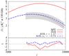 |
Fig. 7 Predictions for the tSZ power spectrum for a weak departure from self-similarity, affecting only the pressure normalization. The red solid line is the tSZ power spectrum given by the A10 pressure model, and the shaded gray region is the 1σ scatter around the best fit Shaw model with SPT data. The blue dashed line represents the A10 model with ϵ = 1.17 (Eq. (12)). The purple dotted line represents A10 model with αz = −0.73 (Eq. (11)). Both parameters, ϵ and αz, modify the redshift evolution of the pressure profile to reduce its amplitude at high-z. |
4.2.2. Association with fgas and X-ray scaling laws
The pressure-mass, P−M, scaling relation has a direct dependence on the gas mass fraction, fgas:P ∝ fgasE8/3M2/3. This quantity is usually assumed as constant, and the A10 work make no explicit statement on gas mass fraction either. However, the P−M relation used by A10 deviates from the self-similar prediction, having a slightly stronger mass dependence: P ∝ E8/3M2/3 + 0.12. By comparing the A10P−M relation with the self-similar prediction, we can assume that this excess is the result of the gas mass fraction: fgas ∝ M0.12. This is motivated by studies which have found that fgas increases with mass of galaxy groups and clusters (Vikhlinin et al. 2006; Arnaud et al. 2007; Pratt et al. 2009; Sun et al. 2009), since non-gravitational processes (e.g., AGN feedback and star formation) produce a larger impact on galaxy groups than in clusters. Pratt et al. (2009), for example, found a relatively strong mass dependence of fgas in the REXCESS sample: fgas ∝ M0.2; and for low mass regime, Sun et al. (2009) constrained the mass dependence in the range: fgas ∝ M0.16−0.22.
 |
Fig. 8 Predictions for the tSZ power spectrum for a weak departure from self-similarity, factoring in additional mass-dependence for the scaling. The red solid line and the gray shaded regions have the same meaning as in earlier figures. The blue dashed line represents the tSZ power spectrum with αz = −0.73 (Eq. (11)), as in Fig. 7. The green dotted line is given by a modified A10 pressure profile that has double mass dependence: fgas ∝ M0.2 for masses below M500 = 1014h-1M⊙, and fgas ∝ M0.12 above this mass limit. Since this change alone is not enough to reach the SPT constraints, we need to introduce a redshift evolution, the result of which is shown by the magenta dash-dotted line. |
In order to assess the impact of different mass dependence of fgas on the tSZ power spectrum, we introduce two distinct power laws for the mass dependence in the A10 pressure profile (Eq. (9)): fgas ∝ M0.2 and fgas ∝ M0.12 for masses below and above M500 = 1014h-1M⊙, respectively. Figure 8 shows the small effect of this broken power law for mass dependence on the tSZ power spectrum (green-dotted line), which is not enough to explain the discrepancy between tSZ power spectrum predictions and the SPT constraints. This shows that a small departure from the self-similar mass scaling, in accordance with the observational results, is not sufficient to explain the low amplitude of the tSZ power spectrum by itself; one needs to consider a modification to the redshift evolution as well. By using our MCMC method, we found that the necessary evolution is given by: αz = −0.66 ± 0.15,  , and
, and  , with a PTE of 0.79 (shown in Fig. 7 by the magenta dash-dotted line).
4.2.3. fgas evolution vs. X-ray data and simulations
In the previous section we assumed that the weakly non-self-similar P−M scaling used by A10 is due to the fact that fgas has a mass dependence. In a similar manner, the non-self-similar evolution required to explain the discrepancy between the SPT measurements and the theoretical predictions of the tSZ power spectrum Sect. 4.2.1) can be attributed to an evolution in fgas. This assumption is motivated by recent observations that show scaling relations, which have a direct dependency on the fgas, do not always follow a self-similar evolution (see discussion in Böhringer et al. 2012). For example, Reichert et al. (2011) and Hilton et al. (2012) have measured the LX−TX scaling relation in different redshift ranges, and they find it to be non-self-similar.
The X-ray bolometric luminosity scales with fgas as  (13)If we assume that the temperature scaling remains self-similar, this would suggest an evolving baryon fraction in clusters. Thus, our tSZ power spectrum based on an evolving fgas model, following the results from previous Sect. 4.2.2, would suggest
  (14)for the (1 + z)αz scaling, or
  (15)for the E(z)8/3−ϵ scaling. We compare these results with the XCS cluster sample result from Hilton et al. (2012), and also from Reichert et al. (2011) who use an ad-hoc high-z cluster sample. Hilton et al. (2012) have found the scaling for the bolometric luminosity as E-1Lbol ∝ T3.18(1 + z)− 1.7 ± 0.4 or Lbol ∝ T3.18E− 1.2 ± 0.5. The result from Reichert et al. (2011) is a less significant change with redshift for the soft-band luminosity:
  . We see that our results are generally consistent with those from Hilton et al. (2012), but there is disagreement with the Reichert et al. (2011) scaling. What is significant, however, is that the errors on the redshift evolution term from our modeling are similar to those available at present from direct X-ray observations. This illustrates the promise of tSZ power spectrum measurements to constrain cluster scaling relations, and we shall discuss its future prospects in Sect. 5.2.
Currently there are no direct fgas measurement in a mass-limited cluster sample out to high redshifts. The works by Allen et al. (2004, 2008) use carefully selected relaxed clusters from X-ray survey data, where they find that fgas remains practically unchanged with redshift. The results from complete X-ray samples are restricted to low redshifts, for example the REXCESS sample by Pratt et al. (2009). Therefore, we make a comparison with recent results from N-body hydrodynamical simulations of clusters that have aimed at measuring the evolution of the baryonic component. Figure 9 shows a comparison of the fgas from Battaglia et al. (2013), who use hydrodynamical TreePM-SPH simulations including cooling, star-formation, and supernova and AGN feedback, with our results. Clearly both our single power law evolution and the broken mass-dependent evolution models are inconsistent with Battaglia et al. (2013) predictions, which show a negligible change in fgas with redshift.
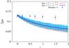 |
Fig. 9 Redshift evolution of the gas mass fraction, fgas, based on our modeling. The blue solid line is for redshift-dependent fgas following the (1 + z)αz power law, and the red dashed line if the same but with two different mass scaling (see Sect. 4.2.2). The hatched and shaded regions mark the 1σ confidence intervals around these lines, respectively. Points with error bars are taken from Battaglia et al. (2013) simulations, who compute the mean fgas within r200. |
4.3. Non-self-similar: an evolving shape of the pressure profile
In our study of a deviation from self-similarity, we have assumed the shape of the pressure profile remains constant with redshift, such that the outer pressure slope parameter β does not change with z. In reality this is unlikely to be true, since the cluster merger fraction steadily increases with redshift, meaning departure from hydrostatic equilibrium should become more significant at high-z, making non-thermal pressure support more prominent. Shaw et al. (2010) considered this effect and identified a redshift evolution of the non-thermal pressure support as potentially the most significant contributor to the lower amplitude of the tSZ power spectrum. An enhancement of the non-thermal pressure (random gas motions) with redshift is also shown by recent hydrodynamical simulations (Lau et al. 2009; Nelson et al. 2014), who in addition find that there is practically no mass dependence for this effect. Our treatment of a non-self-similar pressure shape, therefore, only consists of an evolution with redshift and no scaling with cluster mass.
We consider a model of this redshift-dependent steepening of the pressure profile using a simple, analytic form for the slope parameter β as follows:  (16)Here β0 is the outer slope parameter at z = 0, roughly reminiscent of the low-redshift measurements by A10 and Sun et al. (2011), and βz is its redshift scaling. Figure 10 shows the result of model constraints using this new redshift-dependent term. The parameter βz is highly degenerate with β0, with large errors on their marginalized values:
  and
and  with a PTE = 0.79. Likewise, if we parametrize the redshift evolution of β with an E(z) power-law as
  (17)we obtain
  and
and  with a PTE = 0.76. This parameter degeneracy is a general conclusion whenever we try to constrain a pressure profile model parameter and its redshift evolution simultaneously from the current SPT data.
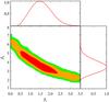 |
Fig. 10 2D Likelihood contours for the correlation between the β0 (the outer slope parameter at z = 0) and βz (its redshift evolution, see Eq. (16)). The colored contours show the 1, 2, and 3σ constraints, and the marginalized values are shown in the side panels. Both β0 and βz tend to lower the tSZ power amplitude and hence anti-correlate. |
5. Discussion and outlook
In this section, we discuss the limitations of the present generation tSZ power spectrum experiments to constrain multiple model parameters for the ICM pressure. We then make predictions for future experiments using simulated bandpower data, based on the same SPT baseline model but scaled to the expected sensitivities for those new tSZ surveys. Finally, we consider the impact of cosmological parameter uncertainties on our methodology of constraining the ICM pressure from current and future tSZ power measurements.
5.1. Need for better tSZ power spectrum measurements
In the course of our modification attempts for the ICM pressure profile from its universal shape and amplitude, we found several potential solutions that can bring the power spectrum amplitude in accordance with the SPT data, but none of these solutions are fully satisfactory in light of the current data or simulations. Evidently, more than one effect is responsible for the observed low tSZ power, such as a combination of steeper pressure profile in the cluster outskirts (and possibly its redshift evolution) and a redshift-dependent baryonic fraction. Unfortunately, current ground- or space-based tSZ experiments do not have the requisite sensitivity and resolution to simultaneously constrain both the shape and the amplitude of the tSZ power spectrum, while separating it from the other multiple astrophysical components affecting the CMB bandpowers at 150 GHz.
As an illustration we pick up the two most prominent parameters featured in our analysis: the slope parameter β and the non-self-similar term αz, to demonstrate this parameter degeneracy. Results are shown in Fig. 11 with colored contours, and marginalized values in red solid lines. When both parameters are varied simultaneously we obtain αz = −1.42 ± 0.75 and β = 4.71 ± 0.71. Clearly, none of these constraints are very informative, the non-self-similar evolution term is consistent with zero at 2σ. A similar case arises for any other parameter combination that can each individually attribute to the lower tSZ power measurement.
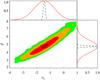 |
Fig. 11 2D likelihood contours for the β and αz parameters and their marginalized values. The colored contours show the 1, 2, and 3σ constraints available from the SPT bandpowers of R12. The black solid lines show the expected constraints from the CCAT tSZ survey. The marginalized errors for CCAT (dashed lines) are almost an order of magnitude smaller. |
Upcoming SZ survey experiments, however, will have sufficient sensitivity and sky-coverage to place simultaneous constraints on the amplitude and the shape of the tSZ power spectrum. This will bring in a significant improvement in the parameter uncertainties (e.g., β or αz), and help to break the current parameter degeneracies. Two such experiments are CCAT1 and SPT-3G. In the following we use CCAT to demonstrate the improved parameter constraints from future SZ experiments.
5.2. Predictions for CCAT
CCAT is expected to be a 25 m class submillimeter telescope that will perform high resolution microwave observations of the Southern sky (e.g., Woody et al. 2012). It will enable accurate measurements of the tSZ and kSZ power spectra in the multipole range between 2000 <ℓ< 20000. CCAT will be more sensitive than SPT in the location of tSZ power spectrum peak, and thus can better constrain the shape and the normalization of the spectrum. Figure 12 shows simulated CCAT bandpowers at 150 GHz from a 5 years survey, performed over 2000 deg2 in approximately 10 000 h of integration. The nominal noise value at 150 GHz for this fiducial CCAT survey is 12 μK/beam. It is assumed that the wide frequency coverage of CCAT, in particular its 850 μm band, will effectively remove the dusty sub-mm galaxy confusion at lower frequencies.
We have used predicted CCAT bandpowers created using the baseline SPT model (C. Reichardt, priv. comm.). Assuming the same shapes for the foreground power spectra templates, the models were extrapolated to higher ℓ values to account for the factor two better resolution of CCAT. For our analysis we also only used the three auto-spectra frequencies (95, 150 and 220 GHz) as in SPT, and the three cross-spectra, since the higher frequencies mostly provide better constraints on the CIB spectra. The survey area was scaled from the SPT survey area used in R12 for improved statistical errors. Calibration and the beam uncertainties were included at 5% level. Although the increased frequency coverage of CCAT might enable a more precise modeling of the CIB background, we did not use any new foreground model for our predictions. The CCAT bandpowers thus reflect an experiment with better sensitivity and resolution but with our current knowledge of the microwave foreground templates.
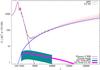 |
Fig. 12 Current SPT bandpower measurements for the total CMB anisotropies (black data points, from R12), and the predicted bandpowers for CCAT (red points), shown with their respective ± 3σ errors. The thick blue line is the best fit SPT foreground model, and the purple line is the lensed CMB power spectrum. The cyan and magenta shaded regions represent the ± 3σ model uncertainties on the tSZ power spectrum from the SPT and CCAT, respectively. This figure illustrates how the improved sensitivity and angular resolution of CCAT can constrain both the amplitude and the shape of the tSZ power spectrum at the same time. |
As seen from Fig. 12, the combination of unprecedented sensitivity and angular resolution of CCAT can constrain the shape and normalization of the tSZ power spectrum accurately, sufficient to break parameter degeneracies. When varying simultaneously the evolution parameter αz and the slope term β, we obtain αz = −1.42 ± 0.07 and β = 4.71 ± 0.08 (see Fig. 11, black contours). The marginalized errors on these two parameters thus show almost an order of magnitude improvement over the current SPT-based results. Similar tight constraints are obtained from other parameter combinations as well. This result is significant, since gaining an order of magnitude better accuracy through targeted observation of galaxy clusters, either in tSZ or in X-rays, will be very difficult, at least with the surveys planned for the coming decade. Through tSZ power spectrum measurements one can thus put the most stringent constraints on the mass and redshift scaling of the pressure profile in galaxy groups and clusters.
We can obtain very similar parameter constraints when using simulated bandpowers for the SPT-3G experiment. SPT-3G is the proposed third generation detector array on SPT (Bender et al. 2014), and will possibly have marginally better sky sensitivity than CCAT due to its longer survey duration. However, its resolution will be worse than the CCAT and may not resolve the shape of the tSZ power equally well. It may also be less efficient in the modeling and removal of foreground components due to a smaller number of submillimeter frequency channels. Nevertheless, as we use the same frequency bands and the same baseline model templates for computing the CCAT and SPT-3G results, the respective model constraints turn out to be very similar. Our results here are not intended as a comparison between experiments, rather as a general demonstration of how these upcoming experiments can help to model cluster astrophysics parameters precisely through the tSZ power spectrum.
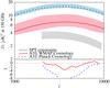 |
Fig. 13 Prediction for the tSZ power spectrum amplitude from the A10 model, but using both the WMAP7 and Planck best fit cosmological model parameters. The higher predicted amplitude from the Planck cosmology comes primarily from the higher values of σ8 and Ωb. The shaded regions around the best-fit models are obtained using the respective parameters chains for these two parameters. The higher sensitivity of Planck clearly provides tighter constraints, although will require more drastic changes to the ICM pressure profile than we considered in this paper. |
5.3. Impact of cosmological uncertainties
The key assumption in our work had been that cosmological parameters like σ8 and Ωm are known to infinite accuracies, which is not realistic. In this final section we discuss the issue of parameter priors instead of fixed values. The error in cosmology can be of two different types. First, there is uncertainty in the cosmological model parameter fits in any given data set (or a combination thereof), that is given by the parameter covariances. Second, there can be additional systematic uncertainties between the best fit values from different probes, like that between the current WMAP and Planck results based on the CMB analysis. In Fig. 13 we show the difference in amplitudes of the tSZ power spectrum, computed using the A10 model without modifications, from either the WMAP7 (Komatsu et al. 2011) or Planck (Planck Collaboration XIII 2015) best fit cosmological parameters. The roughly factor 2 higher amplitude from Planck primarily comes from the higher values of σ8 and Ωb, since the tSZ amplitude roughly scales as  (e.g., R12). Consequently, choosing the present Planck cosmological parameters instead of the WMAP values would require all the pressure profile modification results presented in this paper to be even stronger.
It is not the purpose of this work to address the current tension between the WMAP and Planck cosmological parameters values. However, even if a concordance is reached, there will always remain the statistical uncertainties (and some unresolved systematics) in any specific cosmological model that will affect the pressure model predictions based on the tSZ power. This issue can be addressed through applying known parameter priors in the MCMC chain while computing the halo mass function and the volume element.
We set priors on the two cosmological parameters that affect the tSZ power spectrum most: Ωm and σ8. The priors are from the WMAP9 measurements (Hinshaw et al. 2013), Ωm = 0.264 ± 0.00973 and σ8 = 0.81 ± 0.014, and we take care of the correlation between the parameters by using the actual parameter chains from WMAP9. We run our chains marginalizing over these two parameters, to constrain the redshift evolution parameter αz, as well as the CIB amplitude parameters. We obtain  , whose values and errors are consistent with the ones obtained previously (see Sect. 4.2.1). The use of Planck cosmological priors instead of WMAP9 provides a roughly factor 2 better constraints on these parameters, as can be seen from the respective uncertainty intervals in Fig. 13. A similar conclusion was obtained by Hill & Pajer (2013), who obtained constraints for the outer-slope parameter β at 6−8% level, after marginalizing over cosmology, using a noise power model for Planck .
For the predicted CCAT bandpowers, we constrain the evolution parameter αz in a similar way, with and without priors on the cosmological parameters. For the priors in this case we take a fiducial 1% uncertainty on σ8 and Ωm. This is assuming that by the time when CCAT will be in operation, the constraints on the cosmological parameters will be tighter thanks to some other experiments, like DES or eROSITA2. The results are displayed in Table 2. Clearly, switching from fixed cosmological values to realistic priors makes no major changes in the results, the same being true also for other pressure model parameters. The general conclusions presented in this work remain valid even when the parameter uncertainties are degraded by a factor ~2−3 while marginalizing over the cosmology.
6. Summary and conclusions
We have provided a systematic calibration of intracluster gas models against observational data for the tSZ power spectrum. In particular, we used the GNFW model for an analytical description of the gas pressure profile with empirically determined parameters from Arnaud et al. (2010, A10). We tested various extensions of this model against the SPT measured values of CMB bandpowers on arcminute scales (Reichardt et al. 2012, R12). We employed an MCMC based method following the baseline model of SPT to explore the parameter likelihoods.
Similar to earlier works, we found that the “universal” pressure model of A10 produces an amplitude of the tSZ power spectrum that is roughly a factor two higher than that measured by the SPT, ACT, and Planck. In addition to the A10 model itself, we tested the GNFW models fitted directly to the Planck and Bolocam data, which fail to account for the low tSZ power in the same way as the A10 model. The measurement errors in the Planck and Bolocam results are small compared to the current mismatch between model predictions and experimental results.
We considered three different modifications to the A10 pressure model: first, following a strictly self-similar evolution; second, applying a weakly self-similar evolution where only the amplitude of the pressure profile changes with redshift and mass; and third, having a non-self-similar evolution where both the amplitude and shape of P(r) change with redshift. For the self-similar case, we only varied the cluster outer slope parameter, β, because it has the weakest observational constraint. The maximum likelihood value, which needed to reconcile model predictions with the SPT bandpowers, is β = 6.3 ± 0.2. This is significantly higher than the most probable values measured by the Bolocam and Planck cluster tSZ observation. It also produces low-ℓ tSZ power that is inconsistent with the Planck tSZ bandpower measurements.
In a weak departure from self-similarity, we took the shape of the pressure profile as constant with redshift, but let the amplitude evolve differently than for self-similar models. We considered a power-law dependence of (1 + z) or an additional exponent to E(z) to model this evolution in the pressure scaling. Such a dependence on redshift could be due to an evolution of the gas mass fraction, fgas, with redshift. We found that such models produce an excellent fit to the SPT data. However, an evolution of fgas also affects the X-ray luminosity and would thereby produce some tension with the measured LX−TX scaling relation of high-z clusters. Additionally, a strong decrease in fgas with redshift appears to be inconsistent with some recent hydrodynamical simulations of cosmological halo samples.
In a final attempt to modify the GNFW pressure profile of A10, we let both its shape and amplitude vary with redshift in a strong departure from self-similarity. We considered a simple modeling for the redshift dependence of the pressure outer slope parameter β, as motivated by the recent simulations of random gas motions in the cluster outskirts. We found that in such cases the parameters are highly degenerate: neither the pressure slope at z = 0 nor its redshift evolution can be constrained accurately from the current tSZ power spectrum data.
The degeneracy between the model parameters is a general problem when using the currently available CMB bandpower measurements. For future CMB/tSZ experiments with better sensitivities, these degeneracies can be broken by measuring both the shape and the amplitude of the tSZ power spectrum to high accuracy. We used the simulated bandpower measurements for a CCAT 2000 deg2 sky survey and found almost an order of magnitude improvement over the current model parameter uncertainties. This can, for example, enable simultaneous measurements of the outer slope parameter and the redshift evolution of fgas to the level of a few percent.
We tested the impact of cosmological parameter uncertainties, in particular σ8 and Ωm, on our results. For the current SPT-data based results, we used the WMAP9 cosmological parameter uncertainties, directly using the chains for the relevant cosmological parameters as priors in our MCMC modeling. This degrades the uncertainties on the pressure profile parameters like β or αz by roughly a factor two. For the CCAT fiducial survey, we reduced the cosmological errors by an additional 50%. This causes the ICM pressure model errors for CCAT to degrade roughly by a factor three, which will still be sufficient to place strong constraints on multiple model parameters. The large systematic difference between the current WMAP and Planck cosmological parameters remain an open question, although we note that adopting to the Planck cosmology will roughly cause a factor two higher prediction of the tSZ power amplitude, so will require more drastic modifications to the ICM pressure profile than we considered in this paper.
Acknowledgments
We acknowledge the help from Christian Reichardt and Daisuke Nagai in providing the simulated bandpower measurements for CCAT; Laurie Shaw for sharing his tSZ and kSZ power spectrum templates; and Jack Sayers for sharing the Bolocam cluster pressure profile fit results. The authors acknowledge financial support from the DFG (Deutsche Forschungsgemeinschaft), through the Transregio Programme TR33 “The Dark Universe”. F.P. acknowledges support from BMBF/DLR grant 50 OR 1117.
References
- Allen, S. W., Schmidt, R. W., Ebeling, H., Fabian, A. C., & van Speybroeck, L. 2004, MNRAS, 353, 457 [NASA ADS] [CrossRef] [Google Scholar]
- Allen, S. W., Rapetti, D. A., Schmidt, R. W., et al. 2008, MNRAS, 383, 879 [NASA ADS] [CrossRef] [Google Scholar]
- Arnaud, M., Pointecouteau, E., & Pratt, G. W. 2007, A&A, 474, L37 [NASA ADS] [CrossRef] [EDP Sciences] [Google Scholar]
- Arnaud, M., Pratt, G. W., Piffaretti, R., et al. 2010, A&A, 517, A92 [NASA ADS] [CrossRef] [EDP Sciences] [Google Scholar]
- Battaglia, N., Bond, J. R., Pfrommer, C., Sievers, J. L., & Sijacki, D. 2010, ApJ, 725, 91 [NASA ADS] [CrossRef] [Google Scholar]
- Battaglia, N., Bond, J. R., Pfrommer, C., & Sievers, J. L. 2012a, ApJ, 758, 74 [NASA ADS] [CrossRef] [Google Scholar]
- Battaglia, N., Bond, J. R., Pfrommer, C., & Sievers, J. L. 2012b, ApJ, 758, 75 [NASA ADS] [CrossRef] [Google Scholar]
- Battaglia, N., Bond, J. R., Pfrommer, C., & Sievers, J. L. 2013, ApJ, 777, 123 [NASA ADS] [CrossRef] [Google Scholar]
- Bender, A. N., Cliche, J.-F., de Haan, T., et al. 2014, in SPIE Conf. Ser., 9153, 1 [Google Scholar]
- Bhattacharya, S., Heitmann, K., White, M., et al. 2011, ApJ, 732, 122 [NASA ADS] [CrossRef] [Google Scholar]
- Bhattacharya, S., Nagai, D., Shaw, L., Crawford, T., & Holder, G. P. 2012, ApJ, 760, 5 [NASA ADS] [CrossRef] [Google Scholar]
- Bode, P., Ostriker, J. P., & Vikhlinin, A. 2009, ApJ, 700, 989 [NASA ADS] [CrossRef] [Google Scholar]
- Böhringer, H., Dolag, K., & Chon, G. 2012, A&A, 539, A120 [NASA ADS] [CrossRef] [EDP Sciences] [Google Scholar]
- Borgani, S., Murante, G., Springel, V., et al. 2004, MNRAS, 348, 1078 [NASA ADS] [CrossRef] [Google Scholar]
- de Zotti, G., Ricci, R., Mesa, D., et al. 2005, A&A, 431, 893 [NASA ADS] [CrossRef] [EDP Sciences] [Google Scholar]
- Dunkley, J., Hlozek, R., Sievers, J., et al. 2011, ApJ, 739, 52 [NASA ADS] [CrossRef] [Google Scholar]
- Efstathiou, G., & Migliaccio, M. 2012, MNRAS, 423, 2492 [NASA ADS] [CrossRef] [Google Scholar]
- Fakhouri, O., Ma, C.-P., & Boylan-Kolchin, M. 2010, MNRAS, 406, 2267 [NASA ADS] [CrossRef] [Google Scholar]
- George, E. M., Reichardt, C. L., Aird, K. A., et al. 2015, ApJ, 799, 177 [NASA ADS] [CrossRef] [Google Scholar]
- Giavalisco, M., Steidel, C. C., Adelberger, K. L., et al. 1998, ApJ, 503, 543 [NASA ADS] [CrossRef] [Google Scholar]
- Hall, N. R., Keisler, R., Knox, L., et al. 2010, ApJ, 718, 632 [NASA ADS] [CrossRef] [Google Scholar]
- Hernández-Monteagudo, C., Trac, H., Verde, L., & Jimenez, R. 2006, ApJ, 652, L1 [NASA ADS] [CrossRef] [Google Scholar]
- Hill, J. C., & Pajer, E. 2013, Phys. Rev. D, 88, 063526 [NASA ADS] [CrossRef] [Google Scholar]
- Hilton, M., Romer, A. K., Kay, S. T., et al. 2012, MNRAS, 424, 2086 [NASA ADS] [CrossRef] [Google Scholar]
- Hinshaw, G., Larson, D., Komatsu, E., et al. 2013, ApJS, 208, 19 [NASA ADS] [CrossRef] [Google Scholar]
- Kaiser, N. 1986, MNRAS, 222, 323 [NASA ADS] [CrossRef] [Google Scholar]
- Keisler, R., Reichardt, C. L., Aird, K. A., et al. 2011, ApJ, 743, 28 [NASA ADS] [CrossRef] [Google Scholar]
- Komatsu, E., & Kitayama, T. 1999, ApJ, 526, L1 [NASA ADS] [CrossRef] [PubMed] [Google Scholar]
- Komatsu, E., & Seljak, U. 2002, MNRAS, 336, 1256 [NASA ADS] [CrossRef] [Google Scholar]
- Komatsu, E., Smith, K. M., Dunkley, J., et al. 2011, ApJS, 192, 18 [NASA ADS] [CrossRef] [Google Scholar]
- Lau, E. T., Kravtsov, A. V., & Nagai, D. 2009, ApJ, 705, 1129 [NASA ADS] [CrossRef] [Google Scholar]
- Lueker, M., Reichardt, C. L., Schaffer, K. K., et al. 2010, ApJ, 719, 1045 [NASA ADS] [CrossRef] [Google Scholar]
- Mann, A. W., & Ebeling, H. 2012, MNRAS, 420, 2120 [NASA ADS] [CrossRef] [Google Scholar]
- Maughan, B. J., Giles, P. A., Randall, S. W., Jones, C., & Forman, W. R. 2012, MNRAS, 421, 1583 [NASA ADS] [CrossRef] [Google Scholar]
- McCarthy, I. G., Le Brun, A. M. C., Schaye, J., & Holder, G. P. 2014, MNRAS, 440, 3645 [NASA ADS] [CrossRef] [Google Scholar]
- Nagai, D., Kravtsov, A. V., & Vikhlinin, A. 2007, ApJ, 668, 1 [NASA ADS] [CrossRef] [Google Scholar]
- Navarro, J. F., Frenk, C. S., & White, S. D. M. 1995, MNRAS, 275, 720 [NASA ADS] [CrossRef] [Google Scholar]
- Nelson, K., Lau, E. T., & Nagai, D. 2014, ApJ, 792, 25 [NASA ADS] [CrossRef] [Google Scholar]
- Piffaretti, R., & Valdarnini, R. 2008, A&A, 491, 71 [NASA ADS] [CrossRef] [EDP Sciences] [Google Scholar]
- Planck Collaboration XXXI. 2013, A&A, 550, A131 [NASA ADS] [CrossRef] [EDP Sciences] [Google Scholar]
- Planck Collaboration XII. 2014, A&A, 571, A12 [NASA ADS] [CrossRef] [EDP Sciences] [Google Scholar]
- Planck Collaboration XXI. 2014, A&A, 571, A21 [NASA ADS] [CrossRef] [EDP Sciences] [Google Scholar]
- Planck Collaboration XIII. 2015, A&A, submitted [arXiv:1502.01589] [Google Scholar]
- Pratt, G. W., Croston, J. H., Arnaud, M., & Böhringer, H. 2009, A&A, 498, 361 [NASA ADS] [CrossRef] [EDP Sciences] [Google Scholar]
- Reichardt, C. L., Shaw, L., Zahn, O., et al. 2012, ApJ, 755, 70 [NASA ADS] [CrossRef] [Google Scholar]
- Reichert, A., Böhringer, H., Fassbender, R., & Mühlegger, M. 2011, A&A, 535, A4 [NASA ADS] [CrossRef] [EDP Sciences] [Google Scholar]
- Rubiño-Martín, J. A., & Sunyaev, R. A. 2003, MNRAS, 344, 1155 [NASA ADS] [CrossRef] [Google Scholar]
- Sayers, J., Czakon, N. G., Mantz, A., et al. 2013, ApJ, 768, 177 [NASA ADS] [CrossRef] [Google Scholar]
- Scott, D., & White, M. 1999, A&A, 346, 1 [NASA ADS] [Google Scholar]
- Sehgal, N., Bode, P., Das, S., et al. 2010, ApJ, 709, 920 [NASA ADS] [CrossRef] [Google Scholar]
- Shaw, L. D., Nagai, D., Bhattacharya, S., & Lau, E. T. 2010, ApJ, 725, 1452 [NASA ADS] [CrossRef] [Google Scholar]
- Shaw, L. D., Rudd, D. H., & Nagai, D. 2012, ApJ, 756, 15 [NASA ADS] [CrossRef] [Google Scholar]
- Shi, X., & Komatsu, E. 2014, MNRAS, 442, 521 [NASA ADS] [CrossRef] [Google Scholar]
- Shirokoff, E., Reichardt, C. L., Shaw, L., et al. 2011, ApJ, 736, 61 [NASA ADS] [CrossRef] [Google Scholar]
- Sievers, J. L., Hlozek, R. A., Nolta, M. R., et al. 2013, J. Cosmol. Astropart. Phys., 10, 60 [Google Scholar]
- Suárez-Velásquez, I. F., Mücket, J. P., & Atrio-Barandela, F. 2013, MNRAS, 431, 342 [NASA ADS] [CrossRef] [Google Scholar]
- Sun, M., Voit, G. M., Donahue, M., et al. 2009, ApJ, 693, 1142 [NASA ADS] [CrossRef] [Google Scholar]
- Sun, M., Sehgal, N., Voit, G. M., et al. 2011, ApJ, 727, L49 [NASA ADS] [CrossRef] [Google Scholar]
- Sunyaev, R. A., & Zel’dovich, Y. B. 1972, Comm. Astrophys. Space Phys., 4, 173 [Google Scholar]
- Sunyaev, R. A., & Zel’dovich, Y. B. 1980, MNRAS, 190, 413 [NASA ADS] [CrossRef] [Google Scholar]
- Tinker, J., Kravtsov, A. V., Klypin, A., et al. 2008, ApJ, 688, 709 [NASA ADS] [CrossRef] [Google Scholar]
- Trac, H., Bode, P., & Ostriker, J. P. 2011, ApJ, 727, 94 [NASA ADS] [CrossRef] [Google Scholar]
- Vikhlinin, A., Kravtsov, A., Forman, W., et al. 2006, ApJ, 640, 691 [NASA ADS] [CrossRef] [Google Scholar]
- Voit, G. M. 2005, Adv. Space Res., 36, 701 [Google Scholar]
- Wilson, M. J., Sherwin, B. D., Hill, J. C., et al. 2012, Phys. Rev. D, 86, 122005 [NASA ADS] [CrossRef] [Google Scholar]
- Woody, D., Padin, S., Chauvin, E., et al. 2012, in SPIE Conf. Ser., 8444, 2 [Google Scholar]
Appendix A: Details of the R12 sky model
In this Appendix, we summarize the models defined by Reichardt et al. (2012, R12) for the different components of the microwave sky diffuse emission. These are used as a baseline throughout the article while constraining parameters from the measured SPT bandpowers.
-
Lensed Primary CMB. The lensed CMB is calculated withCAMB3.Gravitational lensing effects are important because they tend toincrease the power of the CMB anisotropies on small angularscales, compared to the unlensed estimates.
-
Poisson infrared (IR) source power. This term takes into account the shot-noise fluctuation power from randomly distributed microwave-emitting galaxies. It is given by
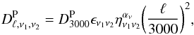 (A.1)where
  is the amplitude of the Poisson power term for infrared galaxies at ℓ = 3000 and at reference frequencies (ν0): 97.9, 153.8, and 219.6 GHz. The coefficient
 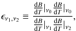 (A.2)is the ratio of power in the ν1 ⊗ ν2 cross-spectrum with respect to the ν0 ⊗ ν0 auto-spectrum.
  is the ratio of the frequencies of the spectrum to the reference frequency. R12 obtained a best fit value for the spectral index of αν = 3.45. B(T) is the CMB blackbody specific intensity.
 -
Clustered IR source power. Because the infrared galaxies trace the mass distribution, they are spatially correlated. This leads to a clustered term in the power spectrum of infrared galaxies given by
 (A.3)where is defined as in the IR Poisson term, and αc = 3.72 is the best fit value taken from R12. Moreover, R12 adopted the power law model ℓ0.8 from Lyman-break correlated galaxies (Giavalisco et al. 1998; Scott & White 1999).
 -
Radio source power. The brightest point sources in the SPT maps coincide with known radio sources. To take this contribution into account, the Poisson radio term is given by
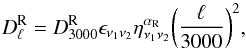 (A.4)where
  is the amplitude of the radio Poisson power spectrum at ℓ = 3000 with value 1.28 ± 0.19 μK2 at 150 GHz. This value is based on the de Zotti et al. (2005) source count model. αR = −0.53 is the mean spectral index from the Shirokoff et al. (2011) analysis.
 -
Galactic cirrus. An average Galactic cirrus contribution term is parametrized as
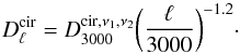 (A.5)Following the cirrus treatment in Hall et al. (2010) and Keisler et al. (2011), R12 measured powers at ℓ = 3000 to be 0.16, 0.21, and 2.19 μK2 for 95, 150, and 220 GHz respectively.
 -
kSZ power spectrum. A homogeneous kSZ power spectrum is adopted, following the cooling plus star-formation (CSF) model of Shaw et al. (2012). This model is constructed by calibrating an analytic model with two hydrodynamical simulations. The CSF template predicts 1.6 μK2 at ℓ = 3000.
-
tSZ power spectrum. R12 uses the analytical model of Shaw et al. (2010) as a template for the tSZ power, which relies on a physical cluster model coupled with halo formalism similar to the one presented in Sect. 2.1. Their cluster model mainly accounts for star formation, energy feedback (from supernovae and active galactic nuclei), and non-thermal pressure support. In our analysis, we replace the Shaw et al. model by a phenomenological description of the intracluster pressure profile that allow us for more freedom.
All Tables
All Figures
|
Fig. 1 2D likelihoods for the power spectra amplitudes at ℓ = 3000 using our MCMC algorithm, compared to the results from R12. The plot shows the tSZ power spectrum ( |
| In the text | |
|
Fig. 2 Discrepancy between the semi-analytic model predictions for the tSZ power and the SPT measurements. The red solid line is the tSZ power spectrum given by the A10 pressure profile (Eq. (9)). The shaded gray region represent the 1σ constraints from the SPT, which is restricted by the shape of the Shaw model (see text for details). The purple dot-dashed line gives the result for the mean GNFW profile as measured by Planck (Planck Collaboration XXXI 2013). The green band marks the corresponding Bolocam measurement (Sayers et al. 2013) with the 68% confidence interval on their model fit parameters. The bottom panel shows the value of χ at each point for these models with respect to the SPT bandpower measurements, in units of the measurement errors in each ℓ-band. |
| In the text | |
|
Fig. 3 Contribution of the tSZ power spectrum in different cluster radial, mass and redshift bins. The plot is in terms of |
| In the text | |
|
Fig. 4 Predictions for the tSZ power spectrum for cluster morphological evolution. The red-solid line is given by the mean A10 pressure profile, the green-dashed line for cool-core clusters, and the blue short-dashed line for non-cool clusters. The purple dot-dashed line shows the relative contribution from the core regions of galaxy clusters (r< 0.2r500) to the total tSZ power, and the dotted line above it factors in an additional scatter contribution (40%) for the core region. This plot shows that, unlike the X-ray luminosity, the core region contributes very little to the tSZ anisotropy power. |
| In the text | |
|
Fig. 5 Predictions for the tSZ power spectrum for self-similar evolution. The red solid line is the tSZ power spectrum given by the A10 pressure profile (Eq. (9)). The shaded gray region represent the 1σ constraints from the SPT based on the Shaw et al. (2010) template (see text for details). The blue dashed line represents the GNFW model with our best fit outer slope (β = 6.35), which provides good fit to the actual SPT data, as shown by the χ plot in the bottom panel. The black data points are the marginalized bandpowers of the Planck tSZ power spectrum, taken from Planck Collaboration XXI (2014). |
| In the text | |
|
Fig. 6 1D likelihood curves for outer slope parameter β. The purple solid line shows the constraints from Planck . Results from Bolocam are shown by the green dashed line. The blue-filled curve represents our best fit constraint on β. |
| In the text | |
|
Fig. 7 Predictions for the tSZ power spectrum for a weak departure from self-similarity, affecting only the pressure normalization. The red solid line is the tSZ power spectrum given by the A10 pressure model, and the shaded gray region is the 1σ scatter around the best fit Shaw model with SPT data. The blue dashed line represents the A10 model with ϵ = 1.17 (Eq. (12)). The purple dotted line represents A10 model with αz = −0.73 (Eq. (11)). Both parameters, ϵ and αz, modify the redshift evolution of the pressure profile to reduce its amplitude at high-z. |
| In the text | |
|
Fig. 8 Predictions for the tSZ power spectrum for a weak departure from self-similarity, factoring in additional mass-dependence for the scaling. The red solid line and the gray shaded regions have the same meaning as in earlier figures. The blue dashed line represents the tSZ power spectrum with αz = −0.73 (Eq. (11)), as in Fig. 7. The green dotted line is given by a modified A10 pressure profile that has double mass dependence: fgas ∝ M0.2 for masses below M500 = 1014h-1M⊙, and fgas ∝ M0.12 above this mass limit. Since this change alone is not enough to reach the SPT constraints, we need to introduce a redshift evolution, the result of which is shown by the magenta dash-dotted line. |
| In the text | |
|
Fig. 9 Redshift evolution of the gas mass fraction, fgas, based on our modeling. The blue solid line is for redshift-dependent fgas following the (1 + z)αz power law, and the red dashed line if the same but with two different mass scaling (see Sect. 4.2.2). The hatched and shaded regions mark the 1σ confidence intervals around these lines, respectively. Points with error bars are taken from Battaglia et al. (2013) simulations, who compute the mean fgas within r200. |
| In the text | |
|
Fig. 10 2D Likelihood contours for the correlation between the β0 (the outer slope parameter at z = 0) and βz (its redshift evolution, see Eq. (16)). The colored contours show the 1, 2, and 3σ constraints, and the marginalized values are shown in the side panels. Both β0 and βz tend to lower the tSZ power amplitude and hence anti-correlate. |
| In the text | |
|
Fig. 11 2D likelihood contours for the β and αz parameters and their marginalized values. The colored contours show the 1, 2, and 3σ constraints available from the SPT bandpowers of R12. The black solid lines show the expected constraints from the CCAT tSZ survey. The marginalized errors for CCAT (dashed lines) are almost an order of magnitude smaller. |
| In the text | |
|
Fig. 12 Current SPT bandpower measurements for the total CMB anisotropies (black data points, from R12), and the predicted bandpowers for CCAT (red points), shown with their respective ± 3σ errors. The thick blue line is the best fit SPT foreground model, and the purple line is the lensed CMB power spectrum. The cyan and magenta shaded regions represent the ± 3σ model uncertainties on the tSZ power spectrum from the SPT and CCAT, respectively. This figure illustrates how the improved sensitivity and angular resolution of CCAT can constrain both the amplitude and the shape of the tSZ power spectrum at the same time. |
| In the text | |
|
Fig. 13 Prediction for the tSZ power spectrum amplitude from the A10 model, but using both the WMAP7 and Planck best fit cosmological model parameters. The higher predicted amplitude from the Planck cosmology comes primarily from the higher values of σ8 and Ωb. The shaded regions around the best-fit models are obtained using the respective parameters chains for these two parameters. The higher sensitivity of Planck clearly provides tighter constraints, although will require more drastic changes to the ICM pressure profile than we considered in this paper. |
| In the text | |
Current usage metrics show cumulative count of Article Views (full-text article views including HTML views, PDF and ePub downloads, according to the available data) and Abstracts Views on Vision4Press platform.
Data correspond to usage on the plateform after 2015. The current usage metrics is available 48-96 hours after online publication and is updated daily on week days.
Initial download of the metrics may take a while.