| Issue |
A&A
Volume 580, August 2015
|
|
|---|---|---|
| Article Number | A20 | |
| Number of page(s) | 24 | |
| Section | Stellar structure and evolution | |
| DOI | https://doi.org/10.1051/0004-6361/201525945 | |
| Published online | 22 July 2015 | |
Massive main-sequence stars evolving at the Eddington limit⋆
Argelander-Insitut für Astronomie, Universität Bonn, Auf dem Hügel 71, 53121 Bonn, Germany
e-mail: This email address is being protected from spambots. You need JavaScript enabled to view it.
Received: 23 February 2015
Accepted: 10 June 2015
Abstract
Context. Massive stars play a vital role in the Universe, however, their evolution even on the main-sequence is not yet well understood.
Aims. Because of the steep mass-luminosity relation, massive main-sequence stars become extremely luminous. This brings their envelopes very close to the Eddington limit. We analyse stellar evolutionary models in which the Eddington limit is reached and exceeded, explore the rich diversity of physical phenomena that take place in their envelopes, and investigate their observational consequences.
Methods. We use published grids of detailed stellar models, computed with a state-of-the-art, one-dimensional hydrodynamic stellar evolution code using LMC composition, to investigate the envelope properties of core hydrogen burning massive stars.
Results. We find that the Eddington limit is almost never reached at the stellar surface, even for stars up to 500 M⊙. When we define an appropriate Eddington limit locally in the stellar envelope, we can show that most stars more massive than ~40 M⊙ actually exceed this limit, in particular, in the partial ionisation zones of iron, helium, or hydrogen. While most models adjust their structure such that the local Eddington limit is exceeded at most by a few per cent, our most extreme models do so by a factor of more than seven. We find that the local violation of the Eddington limit has severe consequences for the envelope structure, as it leads to envelope inflation, convection, density inversions, and, possibly to, pulsations. We find that all models with luminosities higher than 4 × 10⁵L⊙, i.e. stars above ~40 M⊙ show inflation, with a radius increase of up to a factor of about 40. We find that the hot edge of the S Dor variability region coincides with a line beyond which our models are inflated by more than a factor of two, indicating a possible connection between S Dor variability and inflation. Furthermore, our coolest models show highly inflated envelopes with masses of up to several solar masses, and appear to be candidates for producing major luminous blue variable eruptions.
Conclusions. Our models show that the Eddington limit is expected to be reached in all stars above ~40 M⊙ in the LMC, even in lower mass stars in the Galaxy, or in close binaries or rapid rotators. While our results do not support the idea of a direct super-Eddington wind driven by continuum photons, the consequences of the Eddington limit in the form of inflation, pulsations and possibly eruptions may well give rise to a significant enhancement of the time averaged mass-loss rate.
Key words: stars: evolution / stars: interiors / stars: massive / stars: mass-loss
Appendices are available in electronic form at http://www.aanda.org
Present address: Max-Planck-Institut für Astronomie, Königstuhl 17, 69117 Heidelberg, Germany.
© ESO, 2015
1. Introduction
Massive stars are powerful engines and strongly affect the evolution of star-forming galaxies throughout cosmic time (Bresolin et al. 2008). In particular the most massive stars produce copious amounts of ionising photons (Doran et al. 2013), emit powerful stellar winds (e.g. Kudritzki & Puls 2000; Smith 2014) and, in their final explosions, are suspected to produce the most energetic and spectacular stellar explosions, as pair-instability supernovae (Kozyreva et al. 2014), superluminous supernovae (Gal-Yam et al. 2009), and long-duration gamma-ray bursts (Larsson et al. 2007; Raskin et al. 2008).
Massive main-sequence stars, which we understand here as those that undergo core hydrogen burning, have a much higher luminosity than the Sun, as they are known to obey a simple mass-luminosity relation, L ~ Mα, with α> 1. However, whereas this relation is very steep near the solar mass (α ≃ 5), it is shown in Kippenhahn & Weigert (1990) that α → 1 for M → ∞. Indeed, Köhler et al. (2015) find α ≃ 1.1 for M = 500 M⊙.
Since the Eddington factor is proportional to L/M, it is debated in the literature whether main-sequence stars of higher and higher initial mass eventually reach the Eddington limit (Langer 1997; Crowther et al. 2010; Maeder et al. 2012). The answer is clearly: yes, they do. Even when only electron scattering is considered as a source of radiative opacity, the Eddington limit corresponds to a luminosity-to-mass ratio of  (Langer & Kudritzki 2014) for hot stars with a solar helium abundance. This is extremely close to the ℛ-values obtained for models of supermassive stars, where this ratio is nearly mass independent (Fuller et al. 1986; Kato 1986). In fact, Kato (1986) showed that zero-age main-sequence (ZAMS) models computed only with electron scattering opacity reach the Eddington limit at a mass of about ~ 105M⊙.
Whether supermassive stars exist is an open question. Also the mass limit of ordinary stars is presently uncertain (Schneider et al. 2014), however, there is ample evidence for stars with initial masses well above 100 M⊙ in the local Universe. A number of close binary stars have been found with component initial masses above 100 M⊙ (Schnurr et al. 2008, 2009; Taylor et al. 2011; Sana et al. 2013). Crowther et al. (2010) proposed initial masses of up to 300 M⊙ for several stars in the LMC, based on their luminosities. Bestenlehner et al. (2014) identified more than a dozen stars more massive than 100 M⊙ from the sample of ~ 1000 OB stars near 30 Doradus, which are analysed in the frame of VLT-Flames Tarantula Survey (Evans et al. 2011). The hydrogen-rich stars among them have measured ℛ-values of up to 4.3. In hot stars with finite metallicity, the ion opacities can easily exceed the electron scattering opacity (Iglesias & Rogers 1996). It is thus to be expected that the true Eddington limit, which accounts for all opacity sources, is located at ℛ-values of 4.3 or below. This implies that these stars should in fact also have reached, or exceeded their Eddington limit.
In this paper, we explore the question of massive main-sequence stars reaching, or exceeding the Eddington limit from the theoretical side. We show by means of detailed stellar models, as described in Sect. 2, that even all stars more massive than ~ 40 M⊙ are found to reach the Eddington limit. In Sect. 3, we demonstrate the need to properly define a local Eddington factor in the stellar interior, which we then use in Sect. 4 to show that when it exceeds the critical value of one, the stellar envelope becomes inflated. We show further in Sects. 5 and 6 that super-Eddington conditions can lead to density inversions and induce convection. We compare our results to previous studies in Sect. 7, and relate them to observations in Sect. 8, before summarising our conclusions in Sect. 9.
2. Stellar models
The grids of the stellar models we used have been published in Brott et al. (2011) and Köhler et al. (2015). We consider only the core hydrogen burning models computed with LMC metallicity. Each stellar evolution sequence computed by Brott et al. (2011) and Köhler et al. (2015) consists of typically 2000 individual stellar models. However, the full amount of data defining a stellar model is only stored for a few dozen time points per sequence, in non-regular intervals. We analyse those stored models. This scheme has the disadvantage that the density of models in the investigated parameter space is not always as high as it should be ideally. Still, as shown below, it allows for a thorough sampling of the considered parameter space, and it is fully consistent with the results already published.
The stellar models were computed with a state-of-the-art, one-dimensional hydrodynamic implicit Lagrangian code (BEC), which incorporates latest input physics (for details, see Braun 1997; Yoon et al. 2006; Brott et al. 2011; Köhler et al. 2015, and references therein). Convection was treated as in the standard non-adiabatic mixing length approach (Böhm-Vitense 1958; Kippenhahn & Weigert 1990) and a mixing length parameter of α = l/Hp = 1.5 (Langer 1991) was adopted, with l and Hp being the mixing length and the pressure scale height, respectively. This value of the mixing length parameter leads to a good representation of the Sun (Suijs et al. 2008), whereas its calibration to multi-dimensional hydrodynamic models shows that it tends to decrease towards lower gravities (Trampedach et al. 2014; Magic et al. 2015). The convective velocities were limited to the local value of the adiabatic sound speed. The contribution of turbulent pressure (de Jager 1984) was neglected, since it is not expected to be important in determining the stellar hydrostatic structure (Stothers 2003). Indeed, our recent study which includes turbulent pressure (Grassitelli et al. in preparation) shows that e.g. for an 80 M⊙ evolutionary sequence, the stellar radius is increased over that of models without turbulent pressure by at most a few per cent at any time during its main-sequence evolution. Rotational mixing of chemical elements, following Heger et al. (2000), and transport of angular momentum by magnetic fields due to the Spruit-Taylor dynamo were also included (Spruit 2002). The efficiency parameters fc and fμ for rotational mixing were set to 0.0228 and 0.1, respectively (Brott et al. 2011). Radiative opacities were interpolated from the OPAL tables (Iglesias & Rogers 1996). The opacity enhancement due to Fe-group elements at T ~ 200 kK plays a vital role in determining the envelope structure in our stellar models. Even though flux-mean opacities are appropriate to study the momentum balance near the stellar photosphere, in the following we only consider the Rosseland mean opacities, which are thought to behave very similarly to the flux-mean opacities especially at an optical depth larger than one.
The outer boundary condition of the stellar models corresponds to a plane-parallel grey atmosphere model on top of the photosphere. In other words, the effective temperature was used as a boundary condition at a Rosseland optical depth of 2/3. The adopted stellar wind mass-loss recipe leads to small, but finite outflow velocities in the outermost layers, which induces a slight deviation from hydrostatic equilibrium.
The mass-loss prescription from Vink et al. (2000, 2001) was employed to account for the winds of O- and B-type stars. Moreover, parameterized mass-loss rates from Nieuwenhuijzen & de Jager (1990) were used on the cooler side of the bi-stability jump, i.e. at effective temperatures less than 22 000 K, if the Nieuwenhuijzen & de Jager (1990) mass-loss rate exceeded that of Vink et al. (2000, 2001). Wolf-Rayet (WR) type mass-loss was accounted for using the empirical prescription from Hamann et al. (1995) divided by a factor of 10 (Yoon et al. 2006), when the surface helium mass fraction became greater than 70%.
Evolutionary sequences of massive stars, with and without rotation, were computed up to an initial mass of 500 M⊙, starting with LMC composition. The initial mass fractions of hydrogen, helium and metals were taken to be 0.7391, 0.2562, and 0.0047 respectively, in accordance with the observations of young massive stars in the LMC (Brott et al. 2011).
3. The Eddington limit
The Eddington limit refers to the condition in which the outwards radiative acceleration in a star balances the inwards gravity, in hydrostatic equilibrium. It is a concept that is thought to apply at the stellar surface, in the sense that if the Eddington limit is exceeded, a mass outflow should arise (Eddington 1926; Owocki et al. 2004). If we denote the gravity as g = GM/r2 and the radiative acceleration mediated through the electron scattering opacity as grad = κeL/ 4πr2, then the classical Eddington factor Γe is defined as  (1)where L,M, and κe are the luminosity, mass, and electron-scattering opacity, respectively, with the physical constants having their usual meaning. The classical Eddington parameter Γe therefore does not depend on the radius r as the inverse r2 scaling in both grad and g cancel out. Whereas Γe is often convenient to consider, it provides a sufficient instability criterion to stars, but not a necessary one because usually the true opacity exceeds the electron scattering opacity significantly and also contributes to the radiative force.
 |
Fig. 1 Different Eddington factors inside a 285 M⊙, non-rotating, main-sequence model with log L/L⊙ = 6.8 and Teff = 46 600 K (cf. Fig. 9 and Appendix A). The shaded areas mark the different convection zones and the hatched area marks the region with a density inversion. The radius of the non-inflated core is denoted as rcore (defined in Sect. 4). The black dashed horizontal line is drawn at Γ = 1 for convenience. |
As it turns out below, even when the Rosseland mean opacities are used, the models we analyse practically never reach the Eddington limit at their surface. Therefore, we instead consider the Eddington factor in the stellar interior as  (2)where M(r) is the Lagrangian mass coordinate, κ(r) is the Rosseland mean opacity, and L(r) is the local luminosity (Langer 1997). However, Γ′(r) > 1 also does not provide a stability limit in the stellar interior because the stellar layers turn convectively unstable following Schwarzschild’s criterion when Γ′(r) → 1 (Joss et al. 1973; Langer 1997). As the luminosity transported by convection does not contribute to the radiative force, we subtract the convective luminosity in the above expression and redefine the Eddington factor as
  (3)For example, near the stellar core where convective energy transport is highly efficient, Γ(r) stays well below unity in spite of Γ′(r) ≫ 1 and no instability, i.e. departure from hydrostatic equilibrium, occurs (see Fig. 1). In the rest of the paper we refer to Γ(r) as the Eddington factor unless explicitly specified otherwise.
Even with this definition, a super-Eddington layer inside a star does not necessarily lead to a departure from hydrostatic equilibrium or a sustained mass outflow. In the outer envelopes of massive stars, non-adiabatic conditions prevail and convective energy transport is highly inefficient, which pushes Γ(r) close to (or above) one. We find that the stellar models counteract this kind of a super-Eddington luminosity by developing a positive gas pressure gradient, thus restoring hydrostatic equilibrium (Langer 1997; Asplund 1998). In these situations, the canonical definition of Ledd being the maximum sustainable radiative luminosity locally in the stellar interior (in hydrostatic equilibrium) breaks down and loses its significance. As we see below, the radiative luminosity beneath the photosphere can be up to a few times the Eddington luminosity.
In Fig. 1, the behaviour of Γ and Γ′ is shown along with the electron-scattering Eddington factor Γe in a 285 M⊙ non-rotating stellar model, which provides an educative example (see Appendix D for further examples). As explained above, Γ′ and Γe are significantly greater than one in the convective core of the star. The indicated sub-surface convection zones are caused by the opacity peaks at T ~ 1.5 × 10⁶ K (deep iron bump) and at T ~ 2 × 10⁵ K (iron bump). Near the bottom of the inflated envelope (r/rcore ≳ 1; see Sect. 4 for the definition of rcore), Γ approaches one and the Fe opacity bump drives convection. An extended region with Γ ≈ 1 follows. A thin shell very close to the photosphere contains the layers with a positive density gradient and with Γ > 1.
 |
Fig. 2 Positions of the analysed stellar models with Γmax> 0.9 in the Hertzsprung-Russell (HR) diagram (coloured dots). Models with Γmax> 1.1 are coloured dark blue. The solid lines show the evolutionary tracks of non-rotating stellar models (Köhler et al. 2015). The initial masses are marked in units of solar mass. The dashed line corresponds to the zero-age main-sequence of the non-rotating models. The hot and the cool edges of the S Dor instability strip from (Smith et al. 2004) are indicated with thick dotted lines. The interior structures of the models marked with yellow diamonds are shown in Appendix D. |
The stellar models have been computed with a hydrodynamic stellar evolution code, however, because of the large time steps required for stellar evolution calculations, non-hydrostatic solutions are suppressed by our numerical scheme. The resulting hydrostatic structures are still valid solutions of the hydrodynamic equations (see Heger et al. 2000; Kozyreva et al. 2014, for the equations to be solved). Models computed with time steps small enough to resolve the hydrodynamic timescale reveal that some, and potentially many of our models are pulsationally unstable, as will be shown in a forthcoming paper. However, in the cases analysed so far, the pulsations saturate and do not lead to a destruction or ejection of the inflated envelopes. In this respect, we consider our analysis of the hydrostatic equilibrium structures as useful.
3.1. Effect of rotation on the Eddington limit
The effect of the centrifugal force on the structure of rotating stellar models has been studied by a number of groups in the past, including Heger et al. (2000) and Maeder & Meynet (2000). This is done by describing the models in a 1D approximation where all variables are taken as averages over isobaric surfaces (Kippenhahn & Thomas 1970). The stellar structure equations are modified to include the effect of the centrifugal force (Endal & Sofia 1976). The equation of hydrostatic equilibrium becomes  (4)and the radiative temperature gradient in the energy transport equation (in the absence of convection) takes the form
  (5)where the quantities fP and fT have the same definition as in Heger et al. (2000). Consequently, the Eddington luminosity gets modified as:
  (6)However, the Eddington factor,
  (7)does not have any explicit dependence on fP and fT because the factor fP/fT cancels out. Therefore formally, the Eddington factor remains unaffected by rotation. Of course, if the internal evolution of a rotating model is changed, for example, by rotational mixing, its Eddington factor is still different from that of the corresponding non-rotating model.
Of course, real stars are three-dimensional and the centrifugal force must affect the hydrostatic stability limit. However, this is expected to be a function of the latitude at the stellar surface, and in a 2D view, the effect is largest at the equator (Langer 1997). To first order, the critical luminosity Lc to unbind matter at the stellar equatorial surface becomes  (8)where vrot and vKep are the stellar equatorial rotation velocity and the corresponding Keplerian value, respectively. However, to compute the effect reliably, the stellar deformation due to rotation as well as the effect of gravity darkening need to be accounted for (Maeder & Meynet 2000; Maeder 2009). To do this realistically for stars near the Eddington limit requires 2D calculations at least.
The implication is that the effect of rotation on the critical stellar luminosity cannot be properly described through the models analysed here. Those models see the same critical luminosity as if rotation was absent. Since mixing of helium in these models is very weak for rotation rates below those required for chemically homogeneous evolution, most of the rotating models evolve very similar to the non-rotating models (Brott et al. 2011; Köhler et al. 2015), and thus merely serve to augment our database.
3.2. The maximum Eddington factor
In our stellar models, we have determined the maximum Eddington factor Γmax over the whole star, i.e Γmax: = max [Γ(r)]. The maximum Eddington factor Γmax generally occurs in the outer envelopes of our models, where convective energy transport is much less efficient than in the deep interior. The variation of Γmax across the upper HR diagram is shown in Fig. 2 for all analysed core hydrogen burning models that have Γmax> 0.9.
Three distinct regions with Γmax> 1 can be identified in Fig. 2, which can be connected to the opacity peaks of iron, helium, and hydrogen. When one of these opacity peaks is situated sufficiently close to the stellar photosphere, the densities in these layers are so small that convective energy transport becomes inefficient. As a consequence, super-Eddington layers develop that are stabilised by a positive (i.e. inwards directed) gradient in density and gas pressure (see Sect. 5 below). The envelope inflation, which occurs when Γmax approaches one, is discussed in Sect. 4.
Figure 3 shows Γmax as a function of the effective temperature for all our models with Γmax> 0.9. The models that have the hydrogen opacity bump close to their photosphere can obtain values of Γmax as high as ~ 7. This manifests itself as a prominent peak around Teff ≈ 5.5 kK. The inset panel shows the much weaker peaks in Γmax due to partial ionisation zones of Fe and HeII, at T/ kK ~ 200 and 50, respectively. The peak caused by the Fe opacity bump may extend to hotter effective temperatures and apply to hot, hydrogen-free Wolf-Rayet stars, which are not part of our model grid.
 |
Fig. 3 Maximum Eddington factor in the analysed stellar models as a function of Teff for all stellar models shown in Fig. 2, i.e. with Γmax> 0.9. The three peaks in Γmax at Teff/ kK of ~55, 25, and 5.5 correspond to the three opacity bumps associated with the ionisation zones of Fe, HeII and H respectively. Inset: models with Γmax> 0.94 and Teff/ kK ≳ 10 kK. The blue horizontal line at Γmax = 1 is drawn for reference. |
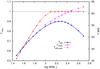 |
Fig. 4 Maximum Eddington factor (Γmax, red line), effective temperature (Teff, blue line) and effective temperature at the non-inflated core (Teff,core, pink line, see Sect. 4, Eq. (10)) as a function of initial mass for the non-rotating ZAMS models. The black dotted line at Γmax = 1 is drawn for reference. |
For stars above about 125 M⊙, Γmax reaches one, even on the ZAMS. This is demonstrated in Fig. 4 which shows both Γmax and effective temperature as a function of mass for the non-rotating stellar models. As these models evolve away from the ZAMS to cooler temperatures, super-Eddington layers develop in their interior. The blue curve shows a maximum effective temperature of 57 000 K at about 200 M⊙, beyond which it starts decreasing with further increase in mass. This behaviour is related to the phenomenon of inflation, which is discussed in detail in Sect. 4. However, the “effective temperature” at the base of the extended, inflated envelope, Teff,core (see Sect. 4), still increases with mass in the whole considered mass range.
3.3. The spectroscopic HR diagram
Figure 5 shows the location of our analysed models in the spectroscopic HR diagram (sHRD, Langer & Kudritzki 2014; Köhler et al. 2015) where instead of the luminosity,  is plotted as a function of the effective temperature. The quantity L can be measured for stars without knowing their distance. Moreover, we have log (L/ L⊙) = ℛ (cf. Sect. 1), such that L is directly proportional to the Eddington factor Γe as
  (9)where g is the surface gravity and the constants have their usual meaning. Therefore one can directly read off Γe (right Y-axis in Fig. 5) from the sHRD. Massive stellar models often evolve with a slowly increasing luminosity over their main-sequence lifetimes. Therefore, where in a conventional HR diagram models with very different Γmax might cluster together (see Fig. 2), they separate out nicely in the sHRD since L∝ L/M. The effect of the opacity peaks on the maximum Eddington factor (Γmax) at temperatures corresponding to the three partial ionisation zones (Fe, HeII and H) is seen more clearly in the sHRD in Fig. 5 compared to the ordinary HR diagram (Fig. 2).
We find that for our ZAMS models the electron scattering opacity is κe ≈ 0.34, while the true photospheric opacity κph is around 0.5. Therefore it is expected that the true Eddington limit (Γ = 1) is achieved at about Γe = 0.7 for stellar models that retain the initial hydrogen abundance at the photosphere. Therefore in Fig. 5 we have drawn two horizontal lines corresponding to Γe = 0.7, one assuming the initial hydrogen mass fraction X = 0.74 (green line) and the other assuming X = 0 (red line). While models with helium-enriched photospheres exceed the green line comfortably, even the most helium-enriched models (rotating or otherwise) stay below the red line.
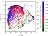 |
Fig. 5 Analysed models shown as coloured dots on the spectroscopic HR diagram (sHRD) with the colour representing the value of Γmax in each model. The Eddington factor Γe (assuming electron scattering opacity only) is directly proportional to the quantity L and is indicated on the right Y-axis for a hydrogen mass fraction of X = 0.74. Some representative evolutionary tracks of non-rotating models, for different initial masses (indicated along the tracks in units of solar mass), are also shown with solid black lines. The green and blue dotted horizontal lines correspond to Γe = 0.7 for X = 0.7 and X = 0, respectively. The colour palette and the models marked with yellow diamonds correspond to those in Fig. 2. The black dashed line roughly divides the sHRD into distinct regions with Γmax> 1 and Γmax< 1. |
From Köhler et al. (2015), we know that models with log L/ L⊙> 4.4 are all hydrogen-deficient, either due to mass-loss or rotationally induced mixing, as both processes lead to an increasing L/M-ratio (cf. their Fig. 18). Figure 5 thus demonstrates that the models that contain super-Eddington layers due to the partial ionisation of helium all have hydrogen deficient envelopes, i.e. they are correspondingly helium-enriched.
Figure 5 reveals that the electron scattering Eddington factor Γe is not a good proxy for the maximum true Eddington factor (Γmax) obtained inside the star. For example, along the horizontal line log L/ L⊙ = 4.3, corresponding to Γe ≃ 0.5, Γmax varies from well below one to values near seven at the cool end. However, we note that below 30 000 K helium and hydrogen recombine, the gas is not fully ionised any more. The line opacities of helium and hydrogen become important, which causes the increase in Γmax (see Figs. 3 and 14).
 |
Fig. 6 HR diagram showing the logarithm of the optical depth τ at the position of Γmax in colour, for all analysed models that have Γmax> 0.9. Some representative evolutionary tracks of non-rotating models, for different initial masses (indicated along the tracks in units of solar mass), are also shown with solid black lines. |
3.4. Surface Eddington factors and the location of Γmax
The optical depth where Γmax is reached gives an idea of how deep in the stellar interior the layer with the highest Eddington factor is located. We investigate this in Fig. 6, which shows that Γmax is located at largely different optical depths in different types of models. While the maximum Eddington factors occur generally at optical depths below ~ 10 000, we see that in the three effective temperature regimes identified by the super-Eddington peaks in Figs. 2 and 3, Γmax can even be located at an optical depth of ~ 10 or below.
For example, when the tracks above log L/L⊙ = 6.2 approach effective temperatures of ~ 30 kK, Γmax is located at the Fe-peak, which is deep inside the envelope (τ ≃ 1400). The models at this stage become helium-rich (Ys ≳ 70%) and the Wolf-Rayet mass-loss prescription is applied. Once these tracks turn bluewards in the HR diagram, the position of Γmax jumps to the helium opacity peak, which is located much closer to the stellar surface. Consequently, we find three orders of magnitude of difference between these two types of models with similar effective temperature and luminosity.
When considering the surface Eddington factors in the sHRD (Fig. 7), we see that only the models with Γ(R⋆) > 0.98 have log L/ L⊙ values of more than 4.6. As discussed above, these models, which started on the main-sequence with initial masses above 300 M⊙ are extremely helium-rich and may correspond to the most extreme late-type WN stars (Sander et al. 2014). As shown in Fig. 8, they exceed the Eddington limit by just a few per mille, which is possible because of the high assumed mass-loss rates that imply a slight deviation from hydrostatic equilibrium near the stellar surface (cf. Sect. 3 above). However, these models are those in which our assumption of an optically thin wind might break down (see Fig. 7 in Köhler et al. 2015). Since the inclusion of an optically thick outflow may lead to changes of the temperature and density structure near the surface, the surface Eddington-factors for these particular models are not reliable.
 |
Fig. 7 Eddington factors at the stellar surface, Γ(R⋆), are shown on the sHRD for our analysed set of models. The models with Γ(R⋆) < 0.9 are indicated with smaller black circles and those with Γ(R⋆) > 0.9 are shown as coloured dots. |
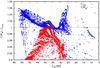 |
Fig. 8 Maximum Eddington factor (Γmax> 0.9) and surface Eddington factor (Γ(R⋆) > 0.9) as a function of the effective temperature Teff of our analysed models. The black dotted line at Γ = 1 is drawn for convenience. |
In summary, we find, on the one hand, that many of our models contain layers at optical depths between a few and a few thousand in which the Eddington factor exceeds the critical value of one. On the other hand, for none of our models we can conclude that the Eddington limit is reached very near to, or at the surface, where for the vast majority we can even exclude that this happens. This finding leads to a shift in the expectation of the response of stars that reach the Eddington limit during their evolution. We might not expect direct outflows driven by super-Eddington luminosities, but instead internal structural changes, in particular envelope inflation.
4. Envelope inflation
Inflation of massive, luminous stars refers to the formation of extended, extremely dilute stellar envelopes. An example of an inflated model is shown in Fig. 9. The red shaded region is the non-inflated core and the blue shaded region is what we refer to as the inflated envelope. In the example, the model is inflated by 60% of its core radius (defined below). In the presented model, the inflated envelope only contain a small fraction of a solar mass, i.e. ≈ 10-5M⊙.
Envelope inflation is inherently different from classical red supergiant formation. The latter occurs after core hydrogen exhaustion, as a consequence of vigorous hydrogen shell burning. This process expands all layers above the shell source, which usually comprise several solar masses in massive stars, and it also operates in low-mass stars, such that no proximity to the Eddington limit is required. The mechanism of envelope inflation that we discuss already works during core hydrogen burning, i.e. even on the ZAMS for sufficiently luminous stars (cf. Fig. 4). Previous investigations have suggested that inflation is related to the proximity of the stellar luminosity to the Eddington luminosity (Ishii et al. 1999; Petrovic et al. 2006; Gräfener et al. 2012) in the envelopes of massive stars with a high luminosity-to-mass ratio (≳ 104L⊙/M⊙). The amount of mass contained in an inflated envelope is usually very small. As we shall see below, inflation, in extreme cases, can also produce core hydrogen burning red supergiants.
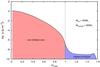 |
Fig. 9 Density profile of a non-rotating 285 M⊙ star with Teff = 46 600 K and log (L/L⊙) = 6.8 (cf. Fig. 1 and Appendix A) showing an inflated envelope and a density inversion. The X-axis has been scaled with the core radius rcore of 25.3 R⊙, as defined in Sect. 4. |
We define inflation in our models through Δr/rcore: = (R⋆−rcore) /rcore, with rcore being the radius at which inflation starts and R⋆, the photospheric radius. Since the densities in inflated envelopes are small, the dominance of radiation pressure in these envelopes is much larger than it is in the main stellar body. We define a model to be inflated if β(r), which is the ratio of gas pressure to total pressure, reaches a value below 0.15 in the interior of a model. The radius at which β goes below 0.15 for the first time from the centre outwards is denoted as rcore, i.e. the start of the inflated region. The remaining extent of the star until the photosphere (R⋆−rcore) is considered the inflated envelope.
We emphasize that our choice of the threshold value for β is arbitrary and not derivable from first principles. However, we have verified that this prescription identifies inflated stars in different parts of the HR diagram very well (cf. Appendix D). As β → 0 for M → ∞, our criterion may fail for extreme masses, however, the mass averaged value of β for the most massive ZAMS model that we analysed (500 M⊙) is 0.3. A threshold value of 0.15 thus appears adequate for the present study. As an example, let us consider a typical inflated model, shown in Appendix A. The value of β in Fig. A.4 decreases sharply at the base of the inflated envelope, to around 0.01. Even if the β threshold is varied by 30%, i.e. 0.15 ± 0.045, the non-inflated core radius rcore changes by only 4%. This goes to show that for clearly inflated models, the value of rcore is insensitive to the threshold value of β.
We furthermore performed a numerical experiment which is suited to show that the core radii identified as described above are indeed robust. We chose an inflated 300 M⊙ model, and then increased the mixing length parameter α such that convection becomes more and more efficient. As shown in Fig. B.1, as a result the extent of the inflated envelope decreased without affecting the model structure inside the core radius, which thus remained independent of α. For α = 40 convection became nearly adiabatic, inflation almost disappeared, and the fact that the photospheric radius in this case became very close to the core radius validates our method of identifying rcore.
 |
Fig. 10 Hertzprung-Russell diagram showing all the core-hydrogen burning inflated models, i.e with Δr/rcore> 0. Models with Δr/rcore> 5 are coloured yellow. Below the solid black line we do not find any inflated models and above the dotted black line we do not find any non-inflated models in our grid. The hot part of the S Dor instability strip is also marked (Smith et al. 2004). |
Figure 10 shows the amount of inflation as defined above, for all our models that fulfil the inflation criterion, in the HR diagram. It reveals that overall, inflation is larger for cooler temperatures. This is not surprising since inflation does not appear to change the stellar luminosity and must therefore induce smaller surface temperatures. We also see that inflation is larger for more luminous stars, which is expected because the Eddington limit is supposed to play a role (see below). We also find inflation increases along the evolutionary tracks of the most massive stars that turn back from the blue supergiant stage, which in this case is due to the shrinking of their core radii. A distinction between the inflated and the non-inflated models is made by drawing the black lines in Fig. 10. They are drawn such that no model is inflated below the solid line and all the models are inflated above the dotted line. In between these two lines we find a mixture of both inflated and non-inflated models. We find that essentially all models above log (L/L⊙) ≃ 5.6 are inflated. Consequently, stars above ~ 40 M⊙ inflate during their main-sequence evolution.
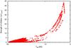 |
Fig. 11 Inflation as a function of the effective temperature for all analysed models that fulfill our inflation criterion. |
Figure 11 shows the inflation factor as function of the stellar effective temperature for our inflated models. Whereas inflation increases the radius of our hot stars by up to a factor of 5, the cool supergiant models can be inflated by a factor of up to 40. We refer to Appendix A for the detailed structures of several inflated models.
In Fig. 12, we take a look at inflation as a function of the core effective temperature Teff,core defined as  (10)where L refers to the surface luminosity and the constants have their usual meaning. We can see that even our coolest models have high core effective temperatures in the sense that if their inflated envelopes were absent their stellar effective temperatures would have been higher than 20 000 K. Those stars with stellar effective temperatures below ~50 000 K contain the He II ionisation zone within their envelopes, and stars with stellar effective temperatures below ~10 000 K also contain the H/He I ionisation zone. However, as revealed by the density and temperature structure of these models (cf. Appendix D), the temperature at the bottom of the inflated envelope is always about 170 000 K, and thus corresponds to the temperature of the iron opacity peak. We conclude that the iron opacity is at least in part driving the inflation of all the stars. For those with cool enough envelopes, helium and hydrogen are likely relevant in addition.
 |
Fig. 12 Inflation as a function of the effective temperature at the core-envelope boundary for all analysed models with Δr/rcore> 0. Colour coding indicates the Teff at the photosphere. |
 |
Fig. 13 Top: inflation (Δr/rcore) as a function of Γmax for the analysed models. The effective temperature of every model is colour-coded. The area within the black dotted lines is magnified below. Bottom: zoomed-in view of the dotted region in the top panel around Γmax = 1. |
4.1. Why do stellar envelopes inflate?
As suggested earlier, the physical cause of inflation in a given star may be its proximity to the Eddington limit. Figure 13 shows the correlation between inflation and Γmax for our models. As expected, we find that our stellar models are not inflated when Γmax is significantly below 1, and they are all inflated for Γmax> 1. Indeed, the top panel of Fig. 13 gives the clear message that the Eddington limit, in the way it is defined in Sect. 3, is likely connected with envelope inflation.
Comparing Fig. 13 (top panel) to Fig. 11 shows that inflation increases up to Teff ≈ 5500 K. Thereafter, Teff and Γmax decrease and the stars keep getting bigger without significant changes in rcore, and, hence, inflation still increases. However, the drop in inflation for the coolest models shows an opposite trend. This is because the non-inflated core radius rcore now moves outwards (increases) such that inflation (Δr/rcore) decreases even though R⋆ keeps increasing (cf. definition of rcore in Sect. 4).
In the zoom-in view shown in the lower panel of Fig. 13, we see some models being inflated for Γmax in the range ~ 0.9...1. Partly, this may be because of the arbitrariness in our definition of inflation. The exact value of Δr/rcore depends somewhat on the choice of the threshold value of β to characterize inflation (cf. Appendix D), i.e. the models with Δr/rcore ≲ 2 and Γmax< 1 may be at the borderline of inflation. The models with Δr/rcore ≲ 2 but Γmax> 1 are all very hot (Teff ≳ 40 000 K) and in those models, the inflation is intrinsically small, but generally unambiguous.
Still, we see a significant number of models below the Eddington limit (Γmax< 1), which show a quite prominent inflation, i.e. which have a radius increase due to inflation of more than a factor of five. We investigated this kind of a model by artificially increasing its mass-loss rate above the critical value Ṁcrit (Petrovic et al. 2006), such that the inflated envelope was removed (cf. Sect. 4.2). We then found that, on turning down the mass-loss rate to its original value, the model regained its initial inflated structure with Γmax< 1. However, Γmax = 1 was reached and exceeded in the course of our experiment. We conclude that a stellar envelope may remain inflated even if the condition Γmax = 1 is not met any more in the course of evolution, but that Γmax ≳ 1 may be required to obtain inflation in the first place.
 |
Fig. 14 Opacity as a function of temperature for fixed values of the opacity parameter R defined as |

In contrast to earlier ideas of a hydrodynamic outflow being triggered when the stellar surface reaches the Eddington limit (Eddington 1926; Owocki et al. 2004), in our models this never happens. When the properly defined Eddington limit is reached inside the envelope, its outermost layers expand hydrostatically and produce inflation. Two possibilities arise in this process. When the star approaches the Eddington limit, the ensuing envelope expansion leads to changes in the temperature and the density structure. Consequently, the envelope opacity can either increase or decrease. Figure 14 shows that the effect of expansion generally leads to a reduced opacity such that the expansion is indeed alleviating the problem. The star then expands until the Eddington limit is just not exceeded any more, which is the reason why we find so many inflated models with Γmax ≃ 1.
Figure 14 shows the OPAL opacities for hydrogen-rich composition for various constant values of R as function of temperature, where R = ρ/ (T/ 106)3. Kippenhahn & Weigert (1990) showed that for constant β = Pgas/P and constant chemical composition, R as a function of spatial co-ordinate inside the star is a constant. Thus, for un-inflated models, the opacity curves in Fig. 14 may closely represent the true run of opacity with temperature inside the star. In the inflated models, β is dropping abruptly at the base of the inflated envelope, which means that the opacity is jumping from a curve with a higher R-value to one with a lower R-value at this location. That is, the opacity is smaller everywhere in the inflated envelope compared to the situation where inflation would not have happened.
For the chemical composition given in Fig. 14 and assuming β ≡ const., we find  (11)such that if β drops from 0.5 in the bulk of the star to 0.1 in the inflated envelope, R drops by one order of magnitude. The corresponding reduction in opacity can be significant, i.e. up to about a factor of two.
When upon expansion the envelope becomes cool enough for another opacity bump to come into play, the problem of not exceeding the Eddington limit might not be solvable this way. Instead, when a new opacity peak is encountered in the outer part of the envelope, super-Eddington conditions occur, i.e. layers with Γmax> 1 (cf. Figs. 2 and 5), along with a strong positive gas pressure (and density) gradient (cf. Sects. 3 and 5). This is most extreme when the envelopes become cool enough (Teff ≲ 8000 K) such that the hydrogen ionisation zone is present in the outer part of the envelope, where Eddington factors of up to seven are achieved.
4.2. Influence of mass-loss on inflation
One might wonder about the sustainability of the inflated layers against mass-loss, which is an important factor in the evolution of metal-rich massive stars. Petrovic et al. (2006) estimated that the inflated envelope cannot be replenished when the mass-loss rate exceeds a critical value of  (12)where M and rcore stand for the stellar mass and the un-inflated radius, respectively, and ρmin is the minimum density in the inflated region. Petrovic et al. (2006) found Ṁcrit ~ 10-5M⊙ yr-1 for a massive hydrogen-free Wolf-Rayet star of 24 M⊙. However, for a typical inflated massive star on the main-sequence (see Fig. A.1), this critical mass-loss rate is of the order 10-3...10-1M⊙ yr-1. These high mass-loss rates are only expected in luminous blue variable (LBV)-type giant eruptions. The mass-loss rates applied to our models are several orders of magnitude smaller (cf. Köhler et al. 2015).
The mass-loss history of four evolutionary sequences without rotation are shown in Fig. 15. Even the 500 M⊙ model never exceeds a mass-loss rate ~ 5 × 10⁻⁴M⊙ yr-1. The critical mass-loss rate for all models shown in Fig. 15 is much higher than the actual mass-loss rates applied. Whereas Ṁcrit typically exceeds Ṁ by a factor of 1000 for the inflated models in the 50 M⊙ sequence, it exceeds that of the 500 M⊙ sequence by a factor of 3...100. It is thus not expected that mass-loss prevents the formation of the inflated envelopes in massive stars near the Eddington limit. In fact, it may be difficult to identify a source of momentum that might drive such strong mass-loss (Shaviv 2001; Owocki et al. 2004). Gräfener et al. (2011) in the Milky Way and Bestenlehner et al. (2014) in the LMC found a steep dependence of the mass-loss rates on the electron-scattering Eddington factor Γe for very massive stars, but they do not find mass-loss rates that substantially exceed 10-4M⊙ yr-1.
 |
Fig. 15 Mass-loss history of four non-rotating evolutionary sequences from our grid. The initial masses are given along each evolutionary track. The colours indicate the different mass-loss prescriptions that were used in different phases, as described in Sect. 2. |
As many of the models analysed here may be pulsationally unstable, the mass-loss rates may be enhanced in this case. Grott et al. (2005) show that hot stars near the Eddington limit may undergo mass-loss due to pulsations, although extreme mass-loss rates are not predicted. For very massive cool stars, on the other hand, Moriya & Langer (2015) find that pulsations may enhance the mass-loss rate to values of the order of 10-2M⊙ yr-1. These extreme values could prevent the corresponding stars to spend a long time on the cool side of the Humphreys-Davidson limit. A detailed consideration of this issue is beyond the scope of the present paper.
5. Density inversions
An inflated envelope can be associated with a “density inversion” near the stellar surface, i.e. a region where the density increases outwards. An example is shown in Fig. 9. In hydrostatic equilibrium, Γ(r) > 1 implies  , and thus
  . As a consequence, all the models that have layers in their envelopes exceeding the Eddington limit show density inversions. The criterion for density inversion can be expressed as (Joss et al. 1973; Paxton et al. 2013)
 ![Mathematical equation: \begin{equation} \frac{L_{\mathrm{rad}}}{L_{\mathrm{Edd}}}>\left[1 + \left(\frac{\partial P_{\mathrm{gas}}}{\partial P_{\mathrm{rad}}}\right)_{\rho} \right]^{-1}, \end{equation}](/articles/aa/full_html/2015/08/aa25945-15/aa25945-15-eq217.png) (13)where Pgas, Prad and ρ stand for the gas pressure, radiation pressure, and density, respectively. A density inversion gives an inwards force and acts as a stabilizing agent for the inflated envelopes. In the above inequality, Pgas is assumed to be a function of ρ and T only, i.e. the mean molecular weight μ is assumed to be constant. Density inversions might also be present in low-mass stars like the Sun where they are caused by the steep increase of μ around the hydrogen recombination zone (cf. Érgma 1971).
(13)where Pgas, Prad and ρ stand for the gas pressure, radiation pressure, and density, respectively. A density inversion gives an inwards force and acts as a stabilizing agent for the inflated envelopes. In the above inequality, Pgas is assumed to be a function of ρ and T only, i.e. the mean molecular weight μ is assumed to be constant. Density inversions might also be present in low-mass stars like the Sun where they are caused by the steep increase of μ around the hydrogen recombination zone (cf. Érgma 1971).
 |
Fig. 16 Upper HR diagram showing all main-sequence models with density inversions. Models with Δρ/ρ> 2 have been coloured yellow. The models without density inversion are indicated with open green triangles. Some representative evolutionary tracks of non-rotating models, for different initial masses (indicated along the tracks in units of solar mass), are also shown with solid coloured lines. |
 |
Fig. 17 Extent of density inversions (Δρ/ρ) as a function of Teff for our models. The three peaks correspond to the three opacity bumps of Fe, HeII, and H in the OPAL tables, as indicated. |
Figure 16 identifies our core hydrogen burning models, which contain a density inversion. The quantity Δρ/ρ represents the strength of the density inversion normalized to the minimum density attained in the inflated zone. We can identify three peaks in Δρ/ρ at Teff/ kK ~ 55, 25, and 5.5 (see also Fig. 17), which coincides exactly with the three Teff-regimes in which models exceed the Eddington limit (cf. Fig. 3). The maximum of the density inversions in the three zones is related to the relative prominence of the three opacity bumps of Fe, HeII, and H respectively, as shown in Fig. 17.
However, an inflated model is not necessarily accompanied by a density inversion. This is depicted clearly in Fig. 18 where we investigate the correlation between inflation and density inversion (this can also be seen by comparing Figs. 10 to 16). Figure 18 shows many models that are even substantially inflated but do not develop a density inversion. The three peaks in the distribution of density inversions of Fig. 17 also show up distinctly in this plot at the three characteristic effective temperatures (shown in colour). Models that show a density inversion do always show some inflation. This is less obvious from Fig. 18 because the hottest models show the smallest amount of inflation (Fig. 11).
 |
Fig. 18 Top: correlation between inflation and density inversions for our models with log L/L⊙> 5. Bottom: zoomed-in view of the area within the back dotted lines in the top panel. |
The stability of density inversions in stellar envelopes has been a matter of debate for the last few decades but there has been no consensus on this issue yet (see Maeder 1992). There have been early speculations by Mihalas (1969) while studying red supergiants that a density inversion might lead to Rayleigh-Taylor instabilities (RTI), resulting in “elephant trunk” structures washing out the positive density gradient. However, as rightly pointed out by Schaerer (1996), RTI does not develop since the effective gravity geff = g(1−Γ) acting on the fluid elements is directed outwards in the super-Eddington layers, which contain the density inversion. Kutter (1970), on the other hand, claimed that a hydrodynamic treatment of the stellar structure equations prevents any density inversion and instead leads to a steady mass outflow. However, this claim is refuted by the present work, since our code solves the 1D hydrodynamic stellar structure equations, in agreement with previous hydrodynamical models by Glatzel & Kiriakidis (1993) and Meynet (1992). Stothers & Chin (1973) suggested that density inversions will lead to strong turbulent motions instead of drastic mass-loss episodes. However, these layers are unstable to convection, so turbulence is present in any case.
Additionally, Glatzel & Kiriakidis (1993) argued in favour of a sustainability of density inversions in the sense that they can be viewed as a natural consequence of strongly non-adiabatic convection, and pointed out that the only plausible way to suppress density inversions is to use a different theory of convection. The only instability expected from simple arguments therefore is convection, which is in line with Wentzel (1970) and Langer (1997).
Still, Ekström et al. (2012) and Yusof et al. (2013) recently considered density inversions as “unphysical”. Density inversions have been suppressed in their models by replacing the pressure scale height in the Mixing Length Theory with the density scale height (cf. Sect. 7). This approach has often been adopted by many investigators in the past to prevent numerical difficulties. As the density scale height tends to infinity when a density inversion starts to develop, this measure tends to enormously increase the convective flux in the relevant layers. It is doubtful whether in reality the convective flux can be increased so much, as the ratio of the local thermal to the local dynamical timescale in the relevant layers is much smaller than one, such that convective eddies lose their thermal energy much faster than they rise, and thus hardly transport any energy at all. Multi-dimensional hydrodynamical simulations would help to settle this issue. We briefly return to this point in Sect. 7.
6. Sub-surface convection
We also studied the convective velocities in the sub-surface convection zones associated with the opacity peaks in our stellar models (Cantiello et al. 2009). We measure these velocities in units of either the isothermal or the adiabatic sound velocity, i.e. cs,ad and cs,iso, respectively, which we compute as  (14)and
 (15)where γ is the adiabatic index, P is the total pressure, ρ is the density, μ is the mean molecular weight, T is the temperature, and kB is the Boltzmann constant. We define Miso as the maximum ratio of the convective velocity over the isothermal sound speed in the stellar envelope, and Mad correspondingly using the adiabatic sound speed.
The true sound speed is in between the adiabatic and isothermal speed, closer to the first one in the inner parts of the star, and closer to the second in the inflated stellar envelope (cf. Sect. 5). In Figs. 19 and 20, we show the values of Miso and Mad for our models in the HR diagram. Whereas the convective velocities are always smaller than the adiabatic sound speed, Fig. 19 shows that the isothermal sound speed can be exceeded locally in our models by a factor of a few. The convective velocity and sound speed profiles for an extreme model are presented in Appendix C.
 |
Fig. 19 Upper HR diagram (log L/L⊙> 5) showing the maximum of the ratio of the convective velocity to the local isothermal sound speed (Miso) of the analysed models as coloured dots. Models with Miso< 1 are shown in black. Some representative evolutionary tracks of non-rotating models, for different initial masses (indicated along the tracks in units of solar mass), are also shown with solid black lines. |
Supersonic convective velocities (adiabatic or isothermal, depending on the physical conditions in the envelope) may not be realistic and are outside the frame of the standard Mixing Length Theory. Therefore, in some of our models, the convective velocities, and thus the convective energy transport, may have been overestimated. A limitation of the velocities to the adequate sound speed is expected to reduce the convective flux, which might lead to further inflation of the stellar envelope.
The cool models, with the strongest inflation, have relatively smaller values of Miso (compared to the hot WR-type models) but large values of Mad (Fig. 20) in the sub-surface convection zones. This is primarily because of the fact that while cs,ad depends on the total pressure, cs,iso only depends on the gas pressure. In the very outer layers of the cool, luminous models, β → 1 and hence Pgas ≈ Ptot. In these situations, cs,ad and cs,iso are only a factor  apart, where γ is the adiabatic index.
 |
Fig. 20 Upper HR diagram (log L/L⊙> 5) showing the maximum of the ratio of the convective velocity to the local adiabatic sound speed Mad of the analysed models (computed with an adiabatic index of 5/3) as coloured dots. Some representative evolutionary tracks of non-rotating models, for different initial masses (indicated along the tracks in units of solar mass), are also shown with solid black lines. |
We find that the convective energy transport is not always negligible in the inflated models (cf. Sect. 4.1). We therefore evaluate the amount of flux that is actually carried by convection in the inflated envelopes of our models. We define the quantity η(Miso) as the fraction of the total flux carried by convection in the stellar envelope, at the location where the isothermal Mach number is the largest. This quantity is plotted as a function of the effective temperature in Fig. 21. It is evident from this figure that η(Miso) need not be small for stellar envelopes to be inflated. However, the hotter a model is the lower its η(Miso)-value at a given luminosity (see Fig. 22). For models hotter than Teff ≈ 63 kK (e.g. the hydrogen-free He stars), η(Miso) indeed goes towards zero (Grassitelli et al., in prep.). The behaviour of the quantity η(Miso) in the HR diagram is shown in Fig. 22.
 |
Fig. 21 Convective efficiency η(Miso), which is the ratio of the convective flux to the total flux at the position where the isothermal Mach number is the largest in the stellar envelope, as a function of the effective temperature for all analysed stellar models in our grid. |
 |
Fig. 22 Upper HR diagram showing all the inflated stellar models in our grid as coloured dots. The convective efficiency η(Miso), which is the ratio of the convective flux to the total flux at the position where the isothermal Mach number is the largest in the stellar envelope, is colour coded. Some representative evolutionary tracks of non-rotating models, for different initial masses (indicated along the tracks in units of solar mass), are also shown with solid black lines. |
7. Comparison with previous studies
7.1. Stellar atmosphere and wind models
Since the Eddington limit was thought to be reached in massive stars near their surface (cf. Sect. 3), several papers have investigated this using stellar atmosphere calculations. Lamers & Fitzpatrick (1988) investigated the Eddington factors in the atmospheres of luminous stars in the temperature-gravity diagram, while Ulmer & Fitzpatrick (1998) did so in the HR diagram. Both studies took the full radiative opacity into account. While their technique did not allow them to reach Eddington factors of one or more, Ulmer and Fitzpatrick found that model atmospheres with a maximum Eddington factor of 0.9 are located near the observed upper luminosity limit of stars in the Large Magellanic Cloud (Humphreys & Davidson 1979; Fitzpatrick & Garmany 1990).
The main feature in the lines of constant Eddington factors in the HR diagram found by Ulmer and Fitzpatrick is a drop from Teff ≃ 60 000 K to 15 000 K. This may correspond to the drop in the maximum Eddington factor seen in our models in the same temperature interval (cf. Figs. 2 and 5). Note that the peak around Teff ≃ 30 000 K in Fig. 3 only corresponds to helium-rich models, which are not considered by Ulmer and Fitzpatrick.
On the other hand, neither inflation nor super-Eddington layers or density inversions are reported by Ulmer and Fitzpatrick, or, to the best of our knowledge, from any hot, main-sequence star model atmosphere calculation so far. One reason might be that many model atmospheres only include a rather limited optical depth range (e.g. up to τ = 100 in Ulmer and Fitzpatrick), such that the iron opacity peak is often not included in the model. Additionally, the computational methods employed might not allow for a non-monotonic density profile.
Given the ubiquity of inflation for models above log L/L⊙> 5.5 or M> 50 M⊙ in the LMC, and a correspondingly lower limit in the Milky Way due to its higher iron content, it is helpful to construct model atmospheres that include this effect and identify its observational signatures. As the density profiles of these kinds of atmospheres near the photosphere are significantly different from those in non-inflated atmospheres, these signatures may indeed be expected.
Asplund (1998) gives a thorough analysis of the Eddington limit in cool star atmosphere models. Indeed, he finds super-Eddington layers and density inversions in his models, and gives arguments for the physically appropriate nature of these phenomena. He also discusses the effects of stellar winds on these features, and finds they may be suppressed by extremely strong winds, but not by winds with mass-loss rates in the observed range. Asplund does not find inflation in his models, again, arguably because the iron opacity peak is not included in his model atmospheres, which appears essential even for our models with cool effective temperatures.
Owocki et al. (2004) and van Marle et al. (2008) studied the winds of stars that reach or exceed the Eddington limit at their surface. As we have shown above, this condition is generally not found in our models (cf. Figs. 7 and 8). However, it may occur in helium-rich stars (see again Fig. 7) and hydrogen-free Wolf-Rayet stars (cf. Heger & Langer 1996), as well as in stars that deviate from thermal or hydrostatic equilibrium. Noticeably, Owocki et al. (2004) find that the mass-loss rates in this case are still quite limited, because of the energy loss attributed to lifting the wind material out of the gravitational potential (see, Heger & Langer 1996).
We want to emphasize in this context that the Eddington limit investigated in the quoted models as well as in our own may be different from the true Eddington limit, because of a number of effects that are all related to the opacity of the stellar matter in the stellar envelopes. One is that convection, which is necessarily present in the layers near or above the Eddington limit, may induce density inhomogeneities or clumping that can alter the effective radiative opacity (Shaviv 1998). In fact, depending on the nature of the clumping, the opacity may be enhanced (Gräfener et al. 2012) or reduced (Owocki et al. 2004; Ruszkowski & Begelman 2003; Muijres et al. 2011). Furthermore, such opacity calculations are tedious, and even in the currently used opacities, important contributions might still be missing.
Finally, the effect of stellar rotation on the stability limit in the atmospheres especially of hot stars is clearly important (Langer 1997, 1998; Maeder & Meynet 2000). However, it adds another dimension to this difficult problem and is therefore generally not included (cf. Sect. 7.2).
7.2. Stellar interior models
The peculiar core-halo density structure of inflated stars was first pointed out by Stothers & Chin (1993), after Iglesias et al. (1992) found the large iron bump in the opacities near 170 000 K. Further studies pointing out this phenomenon comprise Ishii et al. (1999), Petrovic et al. (2006), Gräfener et al. (2012), and Köhler et al. (2015). Conceivably, inflation may be present in further models of very massive stars, but often no statements on the presence or absence of this phenomenon are made in these papers.
For example, the models for very massive stars by Yusof et al. (2013) only discuss the electron-scattering Eddington factor in their models. On the ZAMS, their models are hotter and more compact than those of Köhler et al. (2015) analysed here, which implies that inflation is either weaker or absent. This difference might be due to the different treatment of convection in the sub-surface convective zones, where Yusof et al. (2013) assume the mixing length to be proportional to the density scale height instead of the standard pressure scale height. This prohibits the formation of density inversions, and since the density scale height tends to infinity when a model attempts to establish a density inversion, the convection may transport an arbitrarily large energy flux in this scheme. While the physics of convection introduces one of the biggest uncertainties in the atmospheres of stars close to the Eddington limit, efficient convective energy transport in inflated envelopes appears unlikely (cf. Sect. 5).
A suppression of inflation may have significant consequences for the evolution of massive stars, as the stellar models stay bluer and as a result have lower mass-loss rates and lower spin-down rates. The final fates of these non-inflated stars is significantly different compared to inflated stars (see Köhler et al. 2015, for a detailed discussion).
 |
Fig. 23 HR diagram showing the Köehler et al. models, which include inflation (red) and corresponding non-inflated stellar models (blue) above log L/L⊙> 5 (see text for explanation). The triangles refer to all the Of/WN and WNh single stars studied by Bestenlehner et al. (2014) whereas the black dots and diamonds refer to the B-supergiants (single) from McEvoy et al. (2015) and WN5h stars of the core R136 from Crowther et al. (2010), respectively. The O stars observed within the VFTS survey are marked with crosses (Sabín-Sanjulián et al. 2014; Ramirez-Agudelo et al., in prep.) The ZAMS of the non-rotating stars is marked with the solid line, while the dashed line indicates the approximate position of the ZAMS if inflation was absent (see text for further details). The hot part of the S Doradus instability strip from Smith et al. (2004) is also shown for reference. |
Gräfener et al. (2012) find inflation which, for their models without clumping, correspond well to those of Petrovic et al. (2006) for the Wolf-Rayet case, and to our unpublished solar metallicity main-sequence models, which show a bending of the ZAMS to cool temperatures for M ≳ 100 M⊙. The models of Ishii et al. (1999) also agree very well. Including the work of Stothers & Chin (1993), we conclude that the effect of inflation in models of massive main-sequence stars is found in at least four independent stellar structure codes, with three of them quantitatively producing very similar results.
As pointed out above, massive star evolutionary models, which include effects of rotation, are being produced routinely these days (cf. Maeder & Meynet 2010; Langer 2012; Chieffi & Limongi 2013), but an investigation of the effect of stellar rotation on the stability limit in the atmospheres of hot stars requires the construction of two-dimensional stellar models.
8. Comparison with observations
8.1. The VFTS sample
A prime motivation of Köhler et al. (2015) for computing the evolutionary models for the very massive stars analysed here was to provide a theoretical framework for the VLT Flames-Tarantula Survey (VFTS, Evans et al. 2011). Within VFTS, multi-epoch spectral data of about 700 early B and 300 O stars are being analysed through detailed model atmosphere calculations. Within this effort, Bestenlehner et al. (2014) and McEvoy et al. (2015) derived the physical properties of more than 50 very massive stars, with luminosities log (L/L⊙) > 5.5. We confront the models of Köhler et al. (2015) with this sample in Fig. 23.
Two sets of model data are included in Fig. 23, one that uses the effective temperatures of the Köhler et al. models directly, and a second one where the effective core temperature is used as defined in Sect. 4 (cf. Eq. (10)). The latter approximates the surface temperature of our models if inflation was completely absent. An example calculation presented in Appendix B, where inflation in a 300 M⊙ is suppressed by increasing the mixing length parameter, shows that this approximation is indeed quite good. The ZAMS is also drawn for both sets of models. Note that while wind effects are clearly seen in the spectra of all stars in the sample, the optical depth of their winds is expected not to exceed τ = 2 (cf. Fig. 7 in Köhler et al. 2015) until the stars become very helium rich at their surface. Therefore, the effective temperatures derived from the observations need not be corrected for optically thick winds.
As shown in Bestenlehner et al. (2014), the hottest stars in their sample follow the ZAMS of the Köhler et al. models very closely, well into the regime of inflation. One might expect un-evolved stars to the left of the Köhler et al. ZAMS if inflation was not present. In that case, the stars above log L/L⊙ ≃ 6.2 might spend a significant fraction of their lifetime on the hot side of the Köhler et al. ZAMS. The absence of these hot stars, however, does not conclusively argue that inflation does exist in nature, i.e. even without inflation, the star formation history in 30 Doradus might preclude the existence of stars like this, or they may be hidden in their natal cloud because of their youth (Yorke 1986; Castro et al. 2014).
On the cool side, Fig. 23 shows an absence of observed stars for log L/L⊙ ≳ 6.15 and Teff ≲ 35 000 K. As the evolutionary models predict about 30% of the core hydrogen burning to take place at Teff ≲ 35 000 K in this luminosity regime, which may indicate that the inflation in the models of Köhler et al. is too strong. On the other hand, again, the absence of correspondingly cool stars 30 Doradus may be a result of the local star formation history.
In the luminosity range below, at 5.5 ≲ log L/L⊙ ≲ 6.15, stars as cool as Teff ≲ 15 000 K are observed for which McEvoy et al. (2015) concluded that they are still core hydrogen burning objects. The observed stars are somewhat cooler than the coolest core effective temperature of our models, which may argue in favour of inflation in real stars. Note that the life time of stars in the regime Teff< 20 000 K is only 10% for the Köhler et al. models in the considered luminosity range.
In summary, as the stellar evolution models for these high masses are still quite uncertain, we do not find possible to argue for or against inflation being present in the observed stars considered here based in Fig. 23. In fact, it is intriguing that most of the observed stars are found in the regime where the inflated and non-inflated models overlap. Nevertheless, the observed sample above log L/L⊙ ≃ 5.5 might constitute the best test case, since according to our models, the envelopes of all of them are expected to be strongly affected by the Eddington limit. Model atmosphere calculations for these stars, which include inflation, might shed new light on this question.
8.2. Further possible consequences of inflation
S Doradus type variability
Gräfener et al. (2012) argue that the S Doradus type variability of LBVs may be related to the effect of inflation, and, in particular, focussed on the case of AG Car (Groh et al. 2009). They propose that an instability sets in when their 70 M⊙ chemically homogeneous hydrostatic stellar model is highly inflated (≈ 120 R⊙) by virtue of which the inflated layer becomes gravitationally unbound and a mass-loss episode follows.
In contrast to this idea, our inflated hydrodynamic stellar models do not show any signs of this kind of instability. This could be because of various simplifying assumptions made in the models of Gräfener et al. (2012), in particular, their neglect of the convective flux in the inflated envelopes (cf. Sect. 6). Nevertheless, the physics of convection is very complex in these envelopes, and our results do not necessarily imply that instabilities do not occur.
In fact, considering the hot edge of the S Doradus variability strip, according to Smith et al. (2004), Fig. 22 shows that it roughly separates the models with a low maximum convective efficiency (ηmax< 0.2) from those with a higher convective efficiency. If these high fluxes could not be achieved in these envelopes (cf. Sect. 6), a dynamical instability might well be possible.
The hot edge of the S Doradus variability in the HR diagram also coincides quite well with the borderline separating mildly (Δr/rcore< 1) from strongly (Δr/rcore> 1) inflated models. Comparing this with the observed distribution of very massive stars in Fig. 23, which indicates that essentially no stars are found far to the cool side of this line, could indicate again that strongly inflated envelopes are indeed unstable and might lead to S Doradus type variability and an increased time-averaged mass-loss rate.
LBV eruptions
Glatzel & Kiriakidis (1993) speculated that strange mode pulsations might be responsible for the LBV phenomenon. These pulsations are characterized by very short growth times (~ τdyn) and small brightness fluctuations roughly of the order ~ 10...100 mmag (Glatzel et al. 1999; Grott et al. 2005). However, the mass contained in the pulsating envelopes of their models is negligible compared to the stellar mass, and the associated brightness variations cannot explain the humongous luminosity variations observed in LBV eruptions.
We have seen in Sect. 5 that an inflated envelope often produces a density inversion. These density inversions have been repeatedly proposed as a source of instabilities giving rise to eruptive mass-loss in LBVs (Maeder 1989; Maeder & Conti 1994; Stothers & Chin 1993). Given our results, we consider it unlikely that a density inversion can be the sole cause of LBV eruptions. Density inversions are a generic feature present in a multitude of our models (see Fig. 16), while the LBV phenomenon is quite rare. Furthermore, the density inversions in our models are found very close to the surface of the star with very small amounts of mass above the inversion.
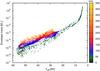 |
Fig. 24 Mass contained in the inflated envelope for all inflated models of our grid, as a function of the effective temperature. The effective actual mass of the models is colour-coded (see colour bar to the right). |
Given our results, inflation per se appears unlikely to cause LBV eruptions, again, because it occurs too abundantly in our models, and also because the mass of the inflated envelope is generally very small. However, Fig. 24 reveals that this is not so for our coolest models. Whereas for most models the mass of the inflated envelope is smaller than ~ 10-3M⊙, intriguingly it rises to several solar masses in the models that have effective temperatures below ~ 10 000 K. These cool models, of which detailed examples are presented in Appendix D, also show the highest Eddington factors (Fig. 3) and the strongest inflation (Fig. 11). This behaviour is seen in the mass range of 40...100 M⊙, which corresponds well to the masses of observed LBVs.
A key feature in our cool models with massive inflated envelopes is visible in Fig. 21. As the opacity in the hydrogen recombination zone becomes very large, effectively blocking any radiation transport, convective efficiencies of the order of η ≃ 1 are needed to transport the stellar luminosity through this zone. Also, in the iron convection zone at the bottom of the envelope, a high convective efficiency (η ≃ 0.5) is found in these models. As shown in Figs. 19 and 20, this requires sonic or even supersonic convective velocities in the framework of the standard MLT as implemented in our code. It thus appears conceivable that in reality convection is less efficient in this kind of a situation, e.g. because of viscous dissipation. When a star enters this region with a massive inflated envelope, throughout which the stellar luminosity can neither be transported by radiation nor by convection, hydrostatic equilibrium is possible any more, and the loosely bound inflated envelope may by dynamically ejected. We believe that this scenario may relate to major LBV eruptions.
As proposed by Langer (2012), a rapid evolutionary timescale of a star may be required to obtain LBV outbursts in addition to the star reaching the Eddington limit. If evolution on the thermal timescale is rapid enough, this might produce LBVs after core hydrogen exhaustion. This rapid evolution may relate to most of the observed LBVs in our Galaxy and the Magellanic Clouds, as well as LBVs after core helium exhaustion, which may address the recently accumulated evidence of LBV outbursts in immediate supernova progenitors (Smith & Arnett 2014).
Supernova shock break-out
A recent study by Moriya et al. (2015) concluded that inflated stellar models can help to explain the extended rise time of the shock break-out signal from the Type Ib supernova SN2008D (Soderberg et al. 2008). In this scenario, the shock break-out occurs deep inside the inflated envelope and consequently the rise time is determined by the radiative diffusion time of the envelope and not the light crossing time. They also noted that more of these kinds of events, if observed in the future, might serve as indicators of inflated supernova progenitors.
Whereas the above result supports the idea that hydrogen-free Wolf-Rayet stars may possess inflated envelopes (Petrovic et al. 2006; Gräfener et al. 2012), LBVs have also been considered to be immediate progenitors of supernovae (Kotak & Vink 2006; Groh et al. 2013). In the realm of high cadence supernova surveys, this opens up the possibility to also test the existence of envelope inflation in hydrogen-rich stars through supernova shock break-out observations.
9. Discussion and conclusions
We investigated the internal structures of the massive star models computed by Brott et al. (2011) and Köhler et al. (2015) using a 1D hydrodynamical stellar evolution code, with particular emphasis on the Eddington limit. We find that the conventional idea of sufficiently massive stars reaching the Eddington limit at the stellar surface is not reproduced by our core hydrogen burning models, not even at 500M⊙ (cf. Figs. 7 and 8). Instead, we find a suitably defined Eddington limit inside the star (Eq. (3)) is reached by models with log (L/L⊙) ≳ 5.6 (Fig. 2), which leads to sub-surface convection, envelope inflation (Fig. 13), and possibly to pulsations. Many of our models even exceed this Eddington limit, and in the extreme case of red supergiants even by factors of up to seven (Fig. 3), with the consequence that strong density inversions develop such that hydrostatic equilibrium is maintained (Fig. 17).
In the analysed models, whose initial composition is chosen to match that of the LMC, all stars above ~ 40 M⊙ reach the Eddington limit in their envelopes. As iron opacities are mainly responsible for this phenomenon, we expect that this mass limit is higher at a lower metallicity, and similarly lower for massive stars in our galaxy. Furthermore, there may be two groups of stars for which this limit comes down even further. First, the centrifugal force in rapidly rotating stars may lead to similar conditions in the envelope layers near the stellar equator, i.e. to a strong latitude dependence of inflation. Perhaps, this could give rise to the so-called B[e] supergiants, which show a slow and dense equatorial wind and a fast polar wind at the same time (Zickgraf et al. 1985). Second, the mass losing stars in interacting close binary systems evolve to much higher L/M-values than corresponding single stars (Langer & Kudritzki 2014), and are therefore expected to reach the Eddington limit for much lower initial masses.
The stability of the inflated envelopes is not investigated here, but many of them are likely to be pulsationally unstable (Glatzel & Kiriakidis 1993; Saio et al. 1998, Sanyal et al., in prep.). If so, it is expected that the pulsations will lead to mass-loss enhancements (e.g. Moriya & Langer 2015), or to the loss of the inflated envelope. In the latter case, the envelope is expected to re-grow unless the achieved time average mass-loss rate exceeds the high critical mass-loss rate (Sect. 4.2). We find that in our coolest models, the mass contained in the inflated envelopes can reach several solar masses (Fig. 24), and speculate that their dynamical loss may resemble LBV major eruptions (cf. Sect. 8.2). Consequently, even though reaching or exceeding the Eddington limit may not immediately lead to strong outflows in stars, clearly the mass-loss rate of the stars is strongly affected, in the sense that the mass-loss is significantly enhanced one way or another.
It will be crucial to test observationally whether luminous, main-sequence stars indeed possess inflated stellar envelopes. This possibility has not yet been investigated with stellar atmosphere models for hot stars. Perhaps the best candidates are the S Doradus variables (Gräfener et al. 2012), which appear in the part of the HR diagram where our models predict a radius inflation by more than a factor of two (cf. Fig. 10).
Finally, we note that besides massive stars, the Eddington limit is relevant to various other types of stars, as luminous post-AGB star, X-ray bursts, Novae, R Corona Borealis stars, and accreting compact objects. It may be interesting to assess to what extent similar phenomena as found in this work might play a role in these objects.
Online material
Appendix A: Interior structure of a 85 M⊙ stellar model
 |
Fig. A.1 Density structure of the stellar model. The black solid line marks the base of the inflated envelope, i.e. where β = 0.15. The intersection of the dotted lines with the red line on either side mark the points where β = 0.15 ± 0.045. |
 |
Fig. A.2 Run of Γ in the interior of the stellar model. |
 |
Fig. A.3 Rosseland mean opacity κ in the interior of the stellar model. |
 |
Fig. A.4 Run of β( = Pgas/Ptot) in the interior of the stellar model. |
 |
Fig. A.5 Fraction of flux carried by radiation (Lrad/Ltot) in the interior of the stellar model. |
Appendix B: Effect of efficient convection on inflation
Knowing that convective flux is proportional to the mixing length, we show here (Fig. B.1) that by increasing the mixing length parameter α in an inflated 300 M⊙ model near the ZAMS, the inflation gradually goes away and what we are left with is an almost non-inflated star, whose radius is well-approximated by core radius rcore of the inflated model.
 |
Fig. B.1 Density profile of a 300 M⊙ model with different values of the mixing length parameter α (see Sect. 2). The black dotted line marks the location of rcore, i.e. the base of the inflated envelope where β = 0.15. |
Appendix C: Convective velocity profile in a WR model
In Fig. C.1, the convective velocity is shown as a function of radius in a massive (147 M⊙) WR-type (YS = 0.89) stellar model.
The variation of isothermal and adiabatic sound speeds are also plotted for comparison. The convective velocities exceed the local isothermal sound speed in the envelope where conditions are non-adiabatic, i.e. the thermal adjustment time is short. In these models, turbulent pressure becomes important (which is not taken into account in our models) as well as standard MLT fails to be a good approximation for modelling convection.
 |
Fig. C.1 Convective velocity, isothermal sound speed, and adiabatic sound speed profiles in a 147 M⊙ WNL type star with Ys = 89%. |
Appendix D: Representative models
The profiles of different relevant physical quantities are shown for a few selected stellar models at five distinct effective temperatures corresponding to the three peaks in Γmax and the two troughs in between the peaks (cf. Fig. 2).
 |
Fig. D.1 Detailed structure examples for stellar models with an effective temperature near 50 000 K, for three different luminosities (cf. Fig. 2). The dashed line marks the point at which β falls below 0.15, i.e. the beginning of the inflated envelope. The square symbol marks the temperature TFe at which κ is maximum because of the iron opacity bump. The hatched regions show the convective zones. |
 |
Fig. D.2 Detailed structure examples for stellar models with an effective temperature near 25 000 K, for three different luminosities (cf. Fig. 2). The dashed line marks the point at which β falls below 0.15, i.e. the beginning of the inflated envelope. The square and the cross mark the temperatures TFe and TFe at which κ is maximum because of the iron and the helium opacity bumps respectively. The hatched regions show the convective zones. |
 |
Fig. D.3 Detailed structure examples for stellar models with an effective temperature near 5000 K, for two different luminosities (cf. Fig. 2). The dashed line marks the point at which β falls below 0.15, i.e. the beginning of the inflated envelope. The square, cross and the circle mark the temperatures TFe, THe, and TH at which κ is maximum because of the iron, helium, and hydrogen opacity bumps respectively. The hatched regions show the convective zones. |
 |
Fig. D.4 Detailed structure examples for stellar models with an effective temperature near 32 000 K, for three different luminosities (cf. Fig. 2). The dashed line marks the point at which β falls below 0.15, i.e. the beginning of the inflated envelope. The square symbol marks the temperature TFe at which κ is maximum because of the iron opacity bump. The hatched regions show the convective zones. |
 |
Fig. D.5 Detailed structure examples for stellar models with an effective temperature near 10 000 K, for three different luminosities (cf. Fig. 2). The dashed line marks the point at which β falls below 0.15, i.e. the beginning of the inflated envelope. The square, cross and the circle mark the temperatures TFe, THe, and TH at which κ is maximum because of the iron, helium, and hydrogen opacity bumps respectively. The hatched regions show the convective zones. |
Acknowledgments
We thank the referee, Raphael Hirschi, for useful comments that improved the manuscript. We are grateful to S. C. Yoon for many fruitful discussions. We also thank C. J. Evans, D. Szécsi, and J. S. Vink for helpful comments on the manuscript. L.G. thanks the International Max Planck Research School for Astronomy and Astrophysics at Bonn.
References
- Asplund, M. 1998, A&A, 330, 641 [NASA ADS] [Google Scholar]
- Bestenlehner, J. M., Gräfener, G., Vink, J. S., et al. 2014, A&A, 570, A38 [NASA ADS] [CrossRef] [EDP Sciences] [Google Scholar]
- Böhm-Vitense, E. 1958, ZAp, 46, 108 [NASA ADS] [Google Scholar]
- Braun, H. 1997, Ph.D. Thesis, , Ludwig-Maximilians-Univ. München [Google Scholar]
- Bresolin, F., Crowther, P. A., & Puls, J. 2008, Massive Stars as Cosmic Engines, IAU Symp., 250 [Google Scholar]
- Brott, I., de Mink, S. E., Cantiello, M., et al. 2011, A&A, 530, A115 [NASA ADS] [CrossRef] [EDP Sciences] [Google Scholar]
- Cantiello, M., Langer, N., Brott, I., et al. 2009, A&A, 499, 279 [NASA ADS] [CrossRef] [EDP Sciences] [Google Scholar]
- Castro, N., Fossati, L., Langer, N., et al. 2014, A&A, 570, L13 [NASA ADS] [CrossRef] [EDP Sciences] [Google Scholar]
- Chieffi, A., & Limongi, M. 2013, ApJ, 764, 21 [NASA ADS] [CrossRef] [Google Scholar]
- Crowther, P. A., Schnurr, O., Hirschi, R., et al. 2010, MNRAS, 408, 731 [NASA ADS] [CrossRef] [Google Scholar]
- de Jager, C. 1984, A&A, 138, 246 [NASA ADS] [Google Scholar]
- Doran, E. I., Crowther, P. A., de Koter, A., et al. 2013, A&A, 558, A134 [NASA ADS] [CrossRef] [EDP Sciences] [Google Scholar]
- Eddington, A. S. 1926, The Internal Constitution of the Stars (Cambridge: Cambridge University Press) [Google Scholar]
- Ekström, S., Georgy, C., Eggenberger, P., et al. 2012, A&A, 537, A146 [NASA ADS] [CrossRef] [EDP Sciences] [Google Scholar]
- Endal, A. S., & Sofia, S. 1976, ApJ, 210, 184 [NASA ADS] [CrossRef] [Google Scholar]
- Érgma, É. 1971, Sov. Astron., 15, 51 [NASA ADS] [Google Scholar]
- Evans, C. J., Taylor, W. D., Hénault-Brunet, V., et al. 2011, A&A, 530, A108 [NASA ADS] [CrossRef] [EDP Sciences] [Google Scholar]
- Fitzpatrick, E. L., & Garmany, C. D. 1990, ApJ, 363, 119 [NASA ADS] [CrossRef] [Google Scholar]
- Fuller, G. M., Woosley, S. E., & Weaver, T. A. 1986, ApJ, 307, 675 [NASA ADS] [CrossRef] [Google Scholar]
- Gal-Yam, A., Mazzali, P., Ofek, E. O., et al. 2009, Nature, 462, 624 [NASA ADS] [CrossRef] [PubMed] [Google Scholar]
- Glatzel, W., & Kiriakidis, M. 1993, MNRAS, 263, 375 [NASA ADS] [Google Scholar]
- Glatzel, W., Kiriakidis, M., Chernigovskij, S., & Fricke, K. J. 1999, MNRAS, 303, 116 [NASA ADS] [CrossRef] [Google Scholar]
- Gräfener, G., Vink, J. S., de Koter, A., & Langer, N. 2011, A&A, 535, A56 [NASA ADS] [CrossRef] [EDP Sciences] [Google Scholar]
- Gräfener, G., Owocki, S. P., & Vink, J. S. 2012, A&A, 538, A40 [NASA ADS] [CrossRef] [EDP Sciences] [Google Scholar]
- Groh, J. H., Hillier, D. J., Damineli, A., et al. 2009, ApJ, 698, 1698 [NASA ADS] [CrossRef] [Google Scholar]
- Groh, J. H., Meynet, G., & Ekström, S. 2013, A&A, 550, L7 [NASA ADS] [CrossRef] [EDP Sciences] [Google Scholar]
- Grott, M., Chernigovski, S., & Glatzel, W. 2005, MNRAS, 360, 1532 [NASA ADS] [CrossRef] [Google Scholar]
- Hamann, W.-R., Koesterke, L., & Wessolowski, U. 1995, A&A, 299, 151 [NASA ADS] [Google Scholar]
- Heger, A., & Langer, N. 1996, A&A, 315, 421 [NASA ADS] [Google Scholar]
- Heger, A., Langer, N., & Woosley, S. E. 2000, ApJ, 528, 368 [NASA ADS] [CrossRef] [Google Scholar]
- Humphreys, R. M., & Davidson, K. 1979, ApJ, 232, 409 [NASA ADS] [CrossRef] [Google Scholar]
- Iglesias, C. A., & Rogers, F. J. 1996, ApJ, 464, 943 [NASA ADS] [CrossRef] [Google Scholar]
- Iglesias, C. A., Rogers, F. J., & Wilson, B. G. 1992, ApJ, 397, 717 [NASA ADS] [CrossRef] [Google Scholar]
- Ishii, M., Ueno, M., & Kato, M. 1999, PASJ, 51, 417 [NASA ADS] [Google Scholar]
- Joss, P. C., Salpeter, E. E., & Ostriker, J. P. 1973, ApJ, 181, 429 [NASA ADS] [CrossRef] [Google Scholar]
- Kato, M. 1986, Ap&SS, 119, 57 [NASA ADS] [CrossRef] [Google Scholar]
- Kippenhahn, R., & Thomas, H.-C. 1970, in Stellar Rotation, ed. A. Slettebak, IAU Colloq., 4, 20 [Google Scholar]
- Kippenhahn, R., & Weigert, A. 1990, Stellar Structure and Evolution (Berlin: Springer) [Google Scholar]
- Köhler, K., Langer, N., de Koter, A., et al. 2015, A&A, 573, A71 [NASA ADS] [CrossRef] [EDP Sciences] [Google Scholar]
- Kotak, R., & Vink, J. S. 2006, A&A, 460, L5 [NASA ADS] [CrossRef] [EDP Sciences] [Google Scholar]
- Kozyreva, A., Yoon, S.-C., & Langer, N. 2014, A&A, 566, A146 [NASA ADS] [CrossRef] [EDP Sciences] [Google Scholar]
- Kudritzki, R.-P., & Puls, J. 2000, ARA&A, 38, 613 [NASA ADS] [CrossRef] [Google Scholar]
- Kutter, G. S. 1970, ApJ, 160, 369 [NASA ADS] [CrossRef] [Google Scholar]
- Lamers, H. J. G. L. M., & Fitzpatrick, E. L. 1988, ApJ, 324, 279 [NASA ADS] [CrossRef] [Google Scholar]
- Langer, N. 1991, A&A, 252, 669 [NASA ADS] [Google Scholar]
- Langer, N. 1997, in Luminous Blue Variables: Massive Stars in Transition, eds. A. Nota, & H. Lamers, ASP Conf. Ser., 120, 83 [Google Scholar]
- Langer, N. 1998, A&A, 329, 551 [NASA ADS] [Google Scholar]
- Langer, N. 2012, ARA&A, 50, 107 [NASA ADS] [CrossRef] [Google Scholar]
- Langer, N., & Kudritzki, R. P. 2014, A&A, 564, A52 [NASA ADS] [CrossRef] [EDP Sciences] [Google Scholar]
- Larsson, J., Levan, A. J., Davies, M. B., & Fruchter, A. S. 2007, MNRAS, 376, 1285 [NASA ADS] [CrossRef] [Google Scholar]
- Maeder, A. 1989, in Physics of Luminous Blue Variables, eds. K. Davidson, A. F. J. Moffat, & H. J. G. L. M. Lamers, IAU Colloq., 113: Astrophys. Space Sci. Lib., 157, 15 [Google Scholar]
- Maeder, A. 1992, in Instabilities in Evolved Super- and Hypergiants, eds. C. de Jager, & H. Nieuwenhuijzen (Amsterdam: North Holland Publ. Corp.), 138 [Google Scholar]
- Maeder, A. 2009, Physics, Formation and Evolution of Rotating Stars (Berlin, Heidelberg: Springer) [Google Scholar]
- Maeder, A., & Conti, P. S. 1994, ARA&A, 32, 227 [NASA ADS] [CrossRef] [Google Scholar]
- Maeder, A., & Meynet, G. 2000, A&A, 361, 159 [NASA ADS] [Google Scholar]
- Maeder, A., & Meynet, G. 2010, New A Rev., 54, 32 [NASA ADS] [CrossRef] [Google Scholar]
- Maeder, A., Georgy, C., Meynet, G., & Ekström, S. 2012, A&A, 539, A110 [NASA ADS] [CrossRef] [EDP Sciences] [Google Scholar]
- Magic, Z., Weiss, A., & Asplund, M. 2015, A&A, 573, A89 [NASA ADS] [CrossRef] [EDP Sciences] [Google Scholar]
- McEvoy, C. M., Dufton, P. L., Evans, C. J., et al. 2015, A&A, 575, A70 [NASA ADS] [CrossRef] [EDP Sciences] [Google Scholar]
- Meynet, G. 1992, in Instabilities in Evolved Super- and Hypergiants, eds. C. de Jager, & H. Nieuwenhuijzen (Amsterdam: North Holland Publ. Corp.), 173 [Google Scholar]
- Mihalas, D. 1969, ApJ, 156, L155 [NASA ADS] [CrossRef] [Google Scholar]
- Moriya, T. J., & Langer, N. 2015, A&A, 573, A18 [NASA ADS] [CrossRef] [EDP Sciences] [Google Scholar]
- Moriya, T. J., Sanyal, D., & Langer, N. 2015, A&A, 575, L10 [Google Scholar]
- Muijres, L. E., de Koter, A., Vink, J. S., et al. 2011, A&A, 526, A32 [Google Scholar]
- Nieuwenhuijzen, H., & de Jager, C. 1990, A&A, 231, 134 [NASA ADS] [Google Scholar]
- Owocki, S. P., Gayley, K. G., & Shaviv, N. J. 2004, ApJ, 616, 525 [NASA ADS] [CrossRef] [Google Scholar]
- Paxton, B., Cantiello, M., Arras, P., et al. 2013, ApJS, 208, 4 [NASA ADS] [CrossRef] [Google Scholar]
- Petrovic, J., Pols, O., & Langer, N. 2006, A&A, 450, 219 [NASA ADS] [CrossRef] [EDP Sciences] [Google Scholar]
- Raskin, C., Scannapieco, E., Rhoads, J., & Della Valle, M. 2008, ApJ, 689, 358 [NASA ADS] [CrossRef] [Google Scholar]
- Ruszkowski, M., & Begelman, M. C. 2003, ApJ, 586, 384 [NASA ADS] [CrossRef] [Google Scholar]
- Sabín-Sanjulián, C., Simón-Díaz, S., Herrero, A., et al. 2014, A&A, 564, A39 [NASA ADS] [CrossRef] [EDP Sciences] [Google Scholar]
- Saio, H., Baker, N. H., & Gautschy, A. 1998, MNRAS, 294, 622 [NASA ADS] [CrossRef] [Google Scholar]
- Sana, H., van Boeckel, T., Tramper, F., et al. 2013, MNRAS, 432, L26 [NASA ADS] [CrossRef] [Google Scholar]
- Sander, A., Todt, H., Hainich, R., & Hamann, W.-R. 2014, A&A, 563, A89 [NASA ADS] [CrossRef] [EDP Sciences] [Google Scholar]
- Schaerer, D. 1996, A&A, 309, 129 [NASA ADS] [Google Scholar]
- Schneider, F. R. N., Izzard, R. G., de Mink, S. E., et al. 2014, ApJ, 780, 117 [NASA ADS] [CrossRef] [Google Scholar]
- Schnurr, O., Casoli, J., Chené, A.-N., Moffat, A. F. J., & St-Louis, N. 2008, MNRAS, 389, L38 [NASA ADS] [CrossRef] [Google Scholar]
- Schnurr, O., Moffat, A. F. J., Villar-Sbaffi, A., St-Louis, N., & Morrell, N. I. 2009, MNRAS, 395, 823 [NASA ADS] [CrossRef] [Google Scholar]
- Shaviv, N. J. 1998, ApJ, 494, L193 [NASA ADS] [CrossRef] [Google Scholar]
- Shaviv, N. J. 2001, ApJ, 549, 1093 [NASA ADS] [CrossRef] [Google Scholar]
- Smith, N. 2014, ARA&A, 52, 487 [NASA ADS] [CrossRef] [MathSciNet] [Google Scholar]
- Smith, N., & Arnett, W. D. 2014, ApJ, 785, 82 [NASA ADS] [CrossRef] [Google Scholar]
- Smith, N., Vink, J. S., & de Koter, A. 2004, ApJ, 615, 475 [NASA ADS] [CrossRef] [Google Scholar]
- Soderberg, A. M., Berger, E., Page, K. L., et al. 2008, Nature, 453, 469 [NASA ADS] [CrossRef] [PubMed] [Google Scholar]
- Spruit, H. C. 2002, A&A, 381, 923 [NASA ADS] [CrossRef] [EDP Sciences] [Google Scholar]
- Stothers, R. B. 2003, ApJ, 589, 960 [NASA ADS] [CrossRef] [Google Scholar]
- Stothers, R., & Chin, C.-W. 1973, ApJ, 179, 555 [NASA ADS] [CrossRef] [Google Scholar]
- Stothers, R. B., & Chin, C.-W. 1993, ApJ, 408, L85 [NASA ADS] [CrossRef] [Google Scholar]
- Suijs, M. P. L., Langer, N., Poelarends, A.-J., et al. 2008, A&A, 481, L87 [NASA ADS] [CrossRef] [EDP Sciences] [Google Scholar]
- Taylor, W. D., Evans, C. J., Sana, H., et al. 2011, A&A, 530, L10 [NASA ADS] [CrossRef] [EDP Sciences] [Google Scholar]
- Trampedach, R., Stein, R. F., Christensen-Dalsgaard, J., Nordlund, Å., & Asplund, M. 2014, MNRAS, 445, 4366 [NASA ADS] [CrossRef] [Google Scholar]
- Ulmer, A., & Fitzpatrick, E. L. 1998, ApJ, 504, 200 [NASA ADS] [CrossRef] [Google Scholar]
- van Marle, A. J., Owocki, S. P., & Shaviv, N. J. 2008, MNRAS, 389, 1353 [NASA ADS] [CrossRef] [Google Scholar]
- Vink, J. S., de Koter, A., & Lamers, H. J. G. L. M. 2000, A&A, 362, 295 [NASA ADS] [Google Scholar]
- Vink, J. S., de Koter, A., & Lamers, H. J. G. L. M. 2001, A&A, 369, 574 [NASA ADS] [CrossRef] [EDP Sciences] [Google Scholar]
- Wentzel, D. G. 1970, ApJ, 160, 373 [NASA ADS] [CrossRef] [Google Scholar]
- Yoon, S., Langer, N., & Norman, C. 2006, A&A, 460, 199 [NASA ADS] [CrossRef] [EDP Sciences] [Google Scholar]
- Yorke, H. W. 1986, ARA&A, 24, 49 [NASA ADS] [CrossRef] [Google Scholar]
- Yusof, N., Hirschi, R., Meynet, G., et al. 2013, MNRAS, 433, 1114 [NASA ADS] [CrossRef] [Google Scholar]
- Zickgraf, F.-J., Wolf, B., Stahl, O., Leitherer, C., & Klare, G. 1985, A&A, 143, 421 [NASA ADS] [Google Scholar]
All Figures
|
Fig. 1 Different Eddington factors inside a 285 M⊙, non-rotating, main-sequence model with log L/L⊙ = 6.8 and Teff = 46 600 K (cf. Fig. 9 and Appendix A). The shaded areas mark the different convection zones and the hatched area marks the region with a density inversion. The radius of the non-inflated core is denoted as rcore (defined in Sect. 4). The black dashed horizontal line is drawn at Γ = 1 for convenience. |
| In the text | |
|
Fig. 2 Positions of the analysed stellar models with Γmax> 0.9 in the Hertzsprung-Russell (HR) diagram (coloured dots). Models with Γmax> 1.1 are coloured dark blue. The solid lines show the evolutionary tracks of non-rotating stellar models (Köhler et al. 2015). The initial masses are marked in units of solar mass. The dashed line corresponds to the zero-age main-sequence of the non-rotating models. The hot and the cool edges of the S Dor instability strip from (Smith et al. 2004) are indicated with thick dotted lines. The interior structures of the models marked with yellow diamonds are shown in Appendix D. |
| In the text | |
|
Fig. 3 Maximum Eddington factor in the analysed stellar models as a function of Teff for all stellar models shown in Fig. 2, i.e. with Γmax> 0.9. The three peaks in Γmax at Teff/ kK of ~55, 25, and 5.5 correspond to the three opacity bumps associated with the ionisation zones of Fe, HeII and H respectively. Inset: models with Γmax> 0.94 and Teff/ kK ≳ 10 kK. The blue horizontal line at Γmax = 1 is drawn for reference. |
| In the text | |
|
Fig. 4 Maximum Eddington factor (Γmax, red line), effective temperature (Teff, blue line) and effective temperature at the non-inflated core (Teff,core, pink line, see Sect. 4, Eq. (10)) as a function of initial mass for the non-rotating ZAMS models. The black dotted line at Γmax = 1 is drawn for reference. |
| In the text | |
|
Fig. 5 Analysed models shown as coloured dots on the spectroscopic HR diagram (sHRD) with the colour representing the value of Γmax in each model. The Eddington factor Γe (assuming electron scattering opacity only) is directly proportional to the quantity L and is indicated on the right Y-axis for a hydrogen mass fraction of X = 0.74. Some representative evolutionary tracks of non-rotating models, for different initial masses (indicated along the tracks in units of solar mass), are also shown with solid black lines. The green and blue dotted horizontal lines correspond to Γe = 0.7 for X = 0.7 and X = 0, respectively. The colour palette and the models marked with yellow diamonds correspond to those in Fig. 2. The black dashed line roughly divides the sHRD into distinct regions with Γmax> 1 and Γmax< 1. |
| In the text | |
|
Fig. 6 HR diagram showing the logarithm of the optical depth τ at the position of Γmax in colour, for all analysed models that have Γmax> 0.9. Some representative evolutionary tracks of non-rotating models, for different initial masses (indicated along the tracks in units of solar mass), are also shown with solid black lines. |
| In the text | |
|
Fig. 7 Eddington factors at the stellar surface, Γ(R⋆), are shown on the sHRD for our analysed set of models. The models with Γ(R⋆) < 0.9 are indicated with smaller black circles and those with Γ(R⋆) > 0.9 are shown as coloured dots. |
| In the text | |
|
Fig. 8 Maximum Eddington factor (Γmax> 0.9) and surface Eddington factor (Γ(R⋆) > 0.9) as a function of the effective temperature Teff of our analysed models. The black dotted line at Γ = 1 is drawn for convenience. |
| In the text | |
|
Fig. 9 Density profile of a non-rotating 285 M⊙ star with Teff = 46 600 K and log (L/L⊙) = 6.8 (cf. Fig. 1 and Appendix A) showing an inflated envelope and a density inversion. The X-axis has been scaled with the core radius rcore of 25.3 R⊙, as defined in Sect. 4. |
| In the text | |
|
Fig. 10 Hertzprung-Russell diagram showing all the core-hydrogen burning inflated models, i.e with Δr/rcore> 0. Models with Δr/rcore> 5 are coloured yellow. Below the solid black line we do not find any inflated models and above the dotted black line we do not find any non-inflated models in our grid. The hot part of the S Dor instability strip is also marked (Smith et al. 2004). |
| In the text | |
|
Fig. 11 Inflation as a function of the effective temperature for all analysed models that fulfill our inflation criterion. |
| In the text | |
|
Fig. 12 Inflation as a function of the effective temperature at the core-envelope boundary for all analysed models with Δr/rcore> 0. Colour coding indicates the Teff at the photosphere. |
| In the text | |
|
Fig. 13 Top: inflation (Δr/rcore) as a function of Γmax for the analysed models. The effective temperature of every model is colour-coded. The area within the black dotted lines is magnified below. Bottom: zoomed-in view of the dotted region in the top panel around Γmax = 1. |
| In the text | |
|
Fig. 14 Opacity as a function of temperature for fixed values of the opacity parameter R defined as |
| In the text | |
|
Fig. 15 Mass-loss history of four non-rotating evolutionary sequences from our grid. The initial masses are given along each evolutionary track. The colours indicate the different mass-loss prescriptions that were used in different phases, as described in Sect. 2. |
| In the text | |
|
Fig. 16 Upper HR diagram showing all main-sequence models with density inversions. Models with Δρ/ρ> 2 have been coloured yellow. The models without density inversion are indicated with open green triangles. Some representative evolutionary tracks of non-rotating models, for different initial masses (indicated along the tracks in units of solar mass), are also shown with solid coloured lines. |
| In the text | |
|
Fig. 17 Extent of density inversions (Δρ/ρ) as a function of Teff for our models. The three peaks correspond to the three opacity bumps of Fe, HeII, and H in the OPAL tables, as indicated. |
| In the text | |
|
Fig. 18 Top: correlation between inflation and density inversions for our models with log L/L⊙> 5. Bottom: zoomed-in view of the area within the back dotted lines in the top panel. |
| In the text | |
|
Fig. 19 Upper HR diagram (log L/L⊙> 5) showing the maximum of the ratio of the convective velocity to the local isothermal sound speed (Miso) of the analysed models as coloured dots. Models with Miso< 1 are shown in black. Some representative evolutionary tracks of non-rotating models, for different initial masses (indicated along the tracks in units of solar mass), are also shown with solid black lines. |
| In the text | |
|
Fig. 20 Upper HR diagram (log L/L⊙> 5) showing the maximum of the ratio of the convective velocity to the local adiabatic sound speed Mad of the analysed models (computed with an adiabatic index of 5/3) as coloured dots. Some representative evolutionary tracks of non-rotating models, for different initial masses (indicated along the tracks in units of solar mass), are also shown with solid black lines. |
| In the text | |
|
Fig. 21 Convective efficiency η(Miso), which is the ratio of the convective flux to the total flux at the position where the isothermal Mach number is the largest in the stellar envelope, as a function of the effective temperature for all analysed stellar models in our grid. |
| In the text | |
|
Fig. 22 Upper HR diagram showing all the inflated stellar models in our grid as coloured dots. The convective efficiency η(Miso), which is the ratio of the convective flux to the total flux at the position where the isothermal Mach number is the largest in the stellar envelope, is colour coded. Some representative evolutionary tracks of non-rotating models, for different initial masses (indicated along the tracks in units of solar mass), are also shown with solid black lines. |
| In the text | |
|
Fig. 23 HR diagram showing the Köehler et al. models, which include inflation (red) and corresponding non-inflated stellar models (blue) above log L/L⊙> 5 (see text for explanation). The triangles refer to all the Of/WN and WNh single stars studied by Bestenlehner et al. (2014) whereas the black dots and diamonds refer to the B-supergiants (single) from McEvoy et al. (2015) and WN5h stars of the core R136 from Crowther et al. (2010), respectively. The O stars observed within the VFTS survey are marked with crosses (Sabín-Sanjulián et al. 2014; Ramirez-Agudelo et al., in prep.) The ZAMS of the non-rotating stars is marked with the solid line, while the dashed line indicates the approximate position of the ZAMS if inflation was absent (see text for further details). The hot part of the S Doradus instability strip from Smith et al. (2004) is also shown for reference. |
| In the text | |
|
Fig. 24 Mass contained in the inflated envelope for all inflated models of our grid, as a function of the effective temperature. The effective actual mass of the models is colour-coded (see colour bar to the right). |
| In the text | |
|
Fig. A.1 Density structure of the stellar model. The black solid line marks the base of the inflated envelope, i.e. where β = 0.15. The intersection of the dotted lines with the red line on either side mark the points where β = 0.15 ± 0.045. |
| In the text | |
|
Fig. A.2 Run of Γ in the interior of the stellar model. |
| In the text | |
|
Fig. A.3 Rosseland mean opacity κ in the interior of the stellar model. |
| In the text | |
|
Fig. A.4 Run of β( = Pgas/Ptot) in the interior of the stellar model. |
| In the text | |
|
Fig. A.5 Fraction of flux carried by radiation (Lrad/Ltot) in the interior of the stellar model. |
| In the text | |
|
Fig. B.1 Density profile of a 300 M⊙ model with different values of the mixing length parameter α (see Sect. 2). The black dotted line marks the location of rcore, i.e. the base of the inflated envelope where β = 0.15. |
| In the text | |
|
Fig. C.1 Convective velocity, isothermal sound speed, and adiabatic sound speed profiles in a 147 M⊙ WNL type star with Ys = 89%. |
| In the text | |
|
Fig. D.1 Detailed structure examples for stellar models with an effective temperature near 50 000 K, for three different luminosities (cf. Fig. 2). The dashed line marks the point at which β falls below 0.15, i.e. the beginning of the inflated envelope. The square symbol marks the temperature TFe at which κ is maximum because of the iron opacity bump. The hatched regions show the convective zones. |
| In the text | |
|
Fig. D.2 Detailed structure examples for stellar models with an effective temperature near 25 000 K, for three different luminosities (cf. Fig. 2). The dashed line marks the point at which β falls below 0.15, i.e. the beginning of the inflated envelope. The square and the cross mark the temperatures TFe and TFe at which κ is maximum because of the iron and the helium opacity bumps respectively. The hatched regions show the convective zones. |
| In the text | |
|
Fig. D.3 Detailed structure examples for stellar models with an effective temperature near 5000 K, for two different luminosities (cf. Fig. 2). The dashed line marks the point at which β falls below 0.15, i.e. the beginning of the inflated envelope. The square, cross and the circle mark the temperatures TFe, THe, and TH at which κ is maximum because of the iron, helium, and hydrogen opacity bumps respectively. The hatched regions show the convective zones. |
| In the text | |
|
Fig. D.4 Detailed structure examples for stellar models with an effective temperature near 32 000 K, for three different luminosities (cf. Fig. 2). The dashed line marks the point at which β falls below 0.15, i.e. the beginning of the inflated envelope. The square symbol marks the temperature TFe at which κ is maximum because of the iron opacity bump. The hatched regions show the convective zones. |
| In the text | |
|
Fig. D.5 Detailed structure examples for stellar models with an effective temperature near 10 000 K, for three different luminosities (cf. Fig. 2). The dashed line marks the point at which β falls below 0.15, i.e. the beginning of the inflated envelope. The square, cross and the circle mark the temperatures TFe, THe, and TH at which κ is maximum because of the iron, helium, and hydrogen opacity bumps respectively. The hatched regions show the convective zones. |
| In the text | |
Current usage metrics show cumulative count of Article Views (full-text article views including HTML views, PDF and ePub downloads, according to the available data) and Abstracts Views on Vision4Press platform.
Data correspond to usage on the plateform after 2015. The current usage metrics is available 48-96 hours after online publication and is updated daily on week days.
Initial download of the metrics may take a while.