| Issue |
A&A
Volume 580, August 2015
|
|
|---|---|---|
| Article Number | A141 | |
| Number of page(s) | 14 | |
| Section | Stellar structure and evolution | |
| DOI | https://doi.org/10.1051/0004-6361/201525856 | |
| Published online | 21 August 2015 | |
Models of red giants in the CoRoT asteroseismology fields combining asteroseismic and spectroscopic constraints
1
School of Physics and Astronomy, University of Birmingham,
Edgbaston, Birmingham
B15 2TT, UK
e-mail:
This email address is being protected from spambots. You need JavaScript enabled to view it.
2
Stellar Astrophysics Centre (SAC), Department of Physics and
Astronomy, Aarhus University, Ny
Munkegade 120, 8000
Aarhus C,
Denmark
3
Geneva Observatory, University of Geneva,
Chemin des Maillettes 51,
1290
Versoix,
Switzerland
4
Institut d’Astrophysique et de Géophysique, Université de
Liège, Allée du 6 Août, Bât.
B5c, 4000
Liège,
Belgium
5
Departement of Physics and Astronomy G. Galilei, University of
Padova, Vicolo dell’Osservatorio
3, 35122
Padova,
Italy
6
LESIA, Observatoire de Paris, PSL Research University, CNRS,
Université Pierre et Marie Curie, Université Denis Diderot,
92195
Meudon Cedex,
France
7
Osservatorio Astronomico di Padova INAF,
Vicolo dell’Osservatorio 5,
35122
Padova,
Italy
8
Laboratório Interinstitucional de e-Astronomia,
LIneA, Rua Gal. Jose Cristino
77, 20921-400
Rio de Janeiro, RJ, Brazil
9
INAF–Osservatorio Astronomico di Brera,
via E. Bianchi 46, 23807
Merate ( LC), Italy
10
Astronomical Institute “Anton Pannekoek”, University of
Amsterdam, Science Park
904, 1098 XH
Amsterdam, The
Netherlands
11
Max-Planck-Institut für Sonnensystemforschung,
Justus-von-Liebig-Weg 3,
37077
Göttingen,
Germany
12
Katholieke Universiteit Leuven, Departement Natuurkunde en
Sterrenkunde, Instituut voor
Sterrenkunde, Celestijnenlaan 200D, 3001
Leuven,
Belgium
13
Institute for Astrophysics, University of Vienna,
Türkenschanzstrasse 17,
1180
Vienna,
Austria
14
Leibniz-Institut für Astrophysik Potsdam (AIP),
An der Sternwarte 16,
14482
Potsdam,
Germany
Received: 10 February 2015
Accepted: 3 May 2015
Abstract
Context. The availability of asteroseismic constraints for a large sample of red giant stars from the CoRoT and Kepler missions paves the way for various statistical studies of the seismic properties of stellar populations.
Aims. We use a detailed spectroscopic study of 19 CoRoT red giant stars to compare theoretical stellar evolution models to observations of the open cluster NGC 6633 and field stars.
Methods. In order to explore the effects of rotation-induced mixing and thermohaline instability, we compare surface abundances of carbon isotopic ratio and lithium with stellar evolution predictions. These chemicals are sensitive to extra-mixing on the red giant branch.
Results. We estimate mass, radius, and distance for each star using the seismic constraints. We note that the Hipparcos and seismic distances are different. However, the uncertainties are such that this may not be significant. Although the seismic distances for the cluster members are self consistent they are somewhat larger than the Hipparcos distance. This is an issue that should be considered elsewhere. Models including thermohaline instability and rotation-induced mixing, together with the seismically determined masses can explain the chemical properties of red giant targets. However, with this sample of stars we cannot perform stringent tests of the current stellar models. Tighter constraints on the physics of the models would require the measurement of the core and surface rotation rates, and of the period spacing of gravity-dominated mixed modes. A larger number of stars with longer times series, as provided by Kepler or expected with Plato, would help ensemble asteroseismology.
Key words: asteroseismology / stars: abundances / stars: evolution / stars: rotation / stars: interiors
© ESO, 2015
1. Introduction
The classical theory of stellar evolution fails to explain abundance anomalies observed in stars ascending the red giant branch (RGB). Indeed, a large number of observations provide compelling evidence of an extra mixing process occurring when the low-mass stars reach the so-called bump in the luminosity function on the RGB. At that point, spectroscopic studies show a drop in the surface carbon isotopic ratio, and the lithium and carbon abundances, while nitrogen abundance increases slightly (e.g. Gilroy & Brown 1991; Gratton et al. 2000; Tautvaišiene et al. 2000; Smiljanic et al. 2009; Tautvaišienė et al. 2013).
A significant effort has been devoted to improving our understanding of the physical processes occurring in low- and intermediate-mass stars. The internal dynamics of these stars is altered by the effects of rotation, through the transport of both angular momentum and chemical species and through the action of meridional circulation and shear turbulence, combined possibly with other processes induced by internal gravity waves or magnetic fields (e.g. Zahn 1992; Maeder & Zahn 1998; Eggenberger et al. 2005; Talon & Charbonnel 1998, 2005; Charbonnel et al. 2013).
Rotation-induced mixing implies a variation of the chemical properties of stars during the main sequence and at the beginning of the RGB, successfully explaining many abundance patterns observed at the surface of low- and intermediate-mass stars (Palacios et al. 2003; Charbonnel & Talon 2008; Smiljanic et al. 2010; Charbonnel & Lagarde 2010). Rotation has also been investigated by several authors as a possible source of mixing during the RGB to explain abundance anomalies observed at the surface of RGB stars (e.g. Sweigart & Mengel 1979; Charbonnel 1995; Denissenkov & Tout 2000; Palacios et al. 2006). However, the total diffusion coefficient of rotation during the RGB is too low to reproduce variations of chemical abundances on the first ascent giant branch as required by spectroscopic observations (e.g. Palacios et al. 2006).
Thermohaline instability driven by 3He-burning has been proposed as a process that is able to modify the photospheric compositions of bright low-mass red giant stars (Charbonnel & Zahn 2007; Charbonnel & Lagarde 2010). This double diffusive instability is induced by the mean molecular weight inversion created, in these stars, by the 3He(3He,2p)4He reaction (included in the pp-chains) in the thin radiative layer between the convective envelope and the hydrogen-burning shell (Eggleton et al. 2006, 2008; Lattanzio et al. 2015). This mechanism has a crucial impact on surface chemical properties of RGB stars in agreement with spectroscopic observations (Charbonnel & Lagarde 2010; Angelou et al. 2011, 2012). It is also very significant for the chemical evolution of light elements in our Galaxy (Lagarde et al. 2011, 2012b).
In summary, and as discussed in Charbonnel & Zahn (2007), Charbonnel & Lagarde (2010), and Lagarde et al. (2011), the effects of both rotation-induced mixing and thermohaline instability explain most of the spectroscopic observations of low- and intermediate-mass stars at various metallicities and evolutionary phases.
Hydrodynamic simulations in 2D and 3D have been used to improve the constraints on the efficiency of thermohaline instability in stellar interiors (Denissenkov et al. 2009; Denissenkov 2010; Denissenkov & Merryfield 2011; Rosenblum et al. 2011; Traxler et al. 2011; Brown et al. 2013). These simulations currently show that double diffusive instability is not efficient enough to significantly change surface abundances (Wachlin et al. 2014). However, they are still far from the parameter space relevant to the stellar regime. Future hydrodynamical simulations representative of conditions met in the stellar interior and taking the coupling of thermohaline instability with other mixing processes into account will shed light on this discrepancy.
Additionally and independent of spectroscopy, the core rotation rate of red giant stars measured by asteroseismology (e.g. Beck et al. 2012; Deheuvels et al. 2012, 2014) shows a significant disagreement with models predictions. It is clear that the physics of red giant models should be improved in the light of new constraints brought by asteroseismology (Eggenberger et al. 2012; Marques et al. 2013).
Seismic properties.
Asteroseismology paves the way to a better understanding of stellar interiors. It provides valuable and independent constraints on current stellar models as well as on the physics of different transport processes. Indeed, for the first time we have the ability to determine the evolutionary state of red giants (e.g. Montalbán et al. 2010; Bedding et al. 2010; Mosser et al. 2011, 2014), to estimate their core rotation rate (e.g. Beck et al. 2012; Deheuvels et al. 2012, 2014), and to deduce the properties of the core He-burning phase (Mosser et al. 2011; Montalbán et al. 2013). Asteroseismology allows us to test stellar evolution models with more stringent constraints for clusters as well as for single stars. With the CoRoT (Baglin et al. 2006) and Kepler (Borucki et al. 2010) space missions, a large number of asteroseismic observations have been obtained for different kinds of stars. They offer a unique opportunity to obtain some fundamental properties by observation of mixed modes in red giants (e.g. Chaplin & Miglio 2013).
To exploit all the potential of asteroseismic data from CoRoT and Kepler missions, it is crucial to combine them with spectroscopic constraints (e.g. Thygesen et al. 2012; Molenda-Zakowicz et al. 2014). The first spectroscopic study of the red giants lying in the asteroseismic CoRoT fields is Morel et al. (2014, hereafter M14). It includes observations of the chemical tracers of extra-mixing in these stars (Li and carbon isotopic ratio). Moreover, this study gives surface chemical properties and seismic properties of three members of NGC 6633, which represents an ideal laboratory for the study of red giant stars at the same age.
In this paper we combine asteroseismic and spectroscopic measurements with stellar evolution models and use them to improve our knowledge of stellar interiors. We propose two complementary approaches to test model predictions of chemical transport with spectroscopic observations, and couple these predictions with seismic constraints on stellar properties. In Sect. 2, we briefly present the observed targets and discuss their stellar properties (radius, mass, and distance). We describe the physical input of the stellar evolution models in Sect. 3.1, while Sect. 3.2 includes a description of the rotation and thermohaline instability effects on the chemical properties of red giant stars. Theoretical predictions are compared to spectroscopic (Li and 12C/13C data) and asteroseismic observations in Sect. 4, before the conclusion in Sect. 5
Chemical properties of stars with 12C/13C data and NGC 6633 members.
2. Stellar parameters
In this section, we estimate the stellar radii and masses using several methods (spectroscopy, asteroseismology, and astrometry) and then we discuss the differences between them. We use the spectroscopic determinations of chemical abundances published by M14. This sample is composed of 19 red giant targets of which 15 were observed by CoRoT including three members of the young open cluster NGC 6633 (HD 170053, HD 170174, HD 170231, see Tables 1 and 2). Morel et al. (2014) also derived the lithium abundances for all the stars in the sample and 12C/13C for four of them (see Table 2). The asteroseismic parameters of large separation, Δν, and frequency of maximum oscillation power, νmax, are also taken from M14. Three different methods were used to obtain these global asteroseismic properties (Mosser & Appourchaux 2009; Hekker et al. 2010; Kallinger et al. 2010a). See Sect. 4 of M14 for more details on the derivations of these parameters. The values are presented in Table 1. We also use the effective temperature derived by M14 using the seismic-surface gravity as a constraint. Astrometric parallaxes from Hipparcos (van Leeuwen 2007, 2009) have been used.
We start by determining radii and masses using seismic scaling relations (Eqs. (1) and (2)):  Solar reference values from M14 are Δν⊙ = 135.1 μHz, νmax, ⊙ = 3090 μHz and Teff, ⊙ = 5777 K.
As the Hipparcos parallax, π, is available for most of the stars studied here, we can derive the stellar luminosity from the apparent magnitude in V-band, and then the stellar radius. The bolometric corrections are derived from Alonso et al. (1999). The extinctions are computed with the 3D Galactic extinction model by Drimmel et al. (2003). If the radius is known, the stellar mass can be estimated from only one of the two global seismic parameters Δν (Eq. (3)) or νmax (Eq. (4)), which allows us to explore any systematic uncertainty on the mass determination:  We can also derive the stellar radius from stellar models using both the spectroscopic and asteroseismic observational data. For this purpose we use PARAM (da Silva et al. 2006; Rodrigues et al. 2014), which computes the stellar properties with a Bayesian approach. This code compares observational data (Teff, [M/H], Δν,νmax) with theoretical models (PARSEC isochrones, Bressan et al. 2012). It also estimates the distances and extinctions by using observed magnitudes in several bandpasses, bolometric corrections (see references in Rodrigues et al. 2014), and by adopting a single extinction curve in terms of V-band. In our case, we use the UBVRI (from SIMBAD) and JHK (2MASS, Cutri et al. 2003) bands, when available.
 |
Fig. 1 Comparison between the radii obtained by different combinations of the available observational constraints. Radii are determined using asteroseismic constraints (νmax,Δν) and Teff (black dots); determined with PARAM (blue crosses); and using the parallax from the Hipparcos catalogue (van Leeuwen 2007), apparent magnitudes, and extinction from different prescriptions (red symbols). Squares represent radii computed with no extinction (AV = 0), and triangles extinctions from the 3D Galactic extinction model by Drimmel et al. (2003). Asterisks indicate stars that are members of NGC 6633. |
 |
Fig. 2 Comparison between the masses obtained by different combinations of the observational constraints available. Masses are determined using asteroseismic constraints (νmax,Δν) and Teff (black dots); using νmax, Teff, the extinction from Drimmel’s model, and the stellar radius from the Hipparcos parallax (using Teff, red triangles); and using Δν and the stellar radius from the Hipparcos parallax (using Teff) and stellar extinction by Drimmel’s model (green squares). Asterisks indicate stars that are members of NGC 6633. |
 |
Fig. 3 Comparison between the distances determined from asteroseismic constraints (νmax,Δν) and Teff (black dots), and the Hipparcos distance (red triangles). In the lower panel, the grey solid line represents the weighted average difference, while the grey dashed lines represent a difference of 25%. Asterisks identify the cluster members. |
Having described the different methods used, we now present a comparison between radii and masses determined using the different combinations of seismic and non-seismic constraints. Radii and masses are computed using Eqs. (1) and (2), and obtained by the other methods (Eqs. (3), (4), and parallax). We also consider extinctions, AV, using Drimmel et al. (2003) as described above, and AV = 0. These results are presented in Figs. 1 and 2.
The radii determined with PARAM have the best precision thanks to the Bayesian approach and the use of priors on stellar evolutionary tracks. In most cases, masses and radii determined using different methods agree within standard uncertainty. However, this is not a very stringent test since the typical uncertainties are ~9% for the radii and ~22% for the masses.
Figure 2 shows a good agreement between red and green symbols. This is mostly due to the strong dependency of the mass estimates (from Eqs. (3) and (4)) on the stellar radius, which in both cases is derived using Hipparcos parallaxes. Miglio et al. (2012) suggested that a relative correction to the scaling relation should be considered between red clump stars and RGB stars, affecting the mass determination of clump stars by ~10%. However, the uncertainties observed here are larger than this correction. Similarly, the correction proposed by Mosser et al. (2013) are smaller (6% for the stellar radius and 3% for the mass).
Figure 3 gives the distance to each star as given in the Hipparcos catalogue, and computed via asteroseismic constraints. The lower panel shows the relative difference between the two quantities. The weighted average of the relative difference between seismic and Hipparcos distances is −0.12 with a statistical uncertainty of 0.03. We used the approach developed by Chaplin et al. (1998) (and used in Miglio et al. 2012) to compute the weighted average of the relative distance and include the Student t-distribution to take into account the small number of points. These marginally significant differences suggest that the seismic distances are overestimated compared to the Hipparcos distances, with consequences for the seismic radii and masses (see Figs. 1 and 2).
The weighted average of the relative difference between Hipparcos and seismic distances for the stars in the cluster is −0.23 ± 0.10. The accuracy of Hipparcos parallaxes has recently been questioned by Melis et al. (2014) in the case of the Pleiades, suggesting that the Hipparcos distance is overestimated by ~12%. However, our current poor knowledge of systematic uncertainties on the seismically determined distances prevents us from contributing to this debate.
3. Theoretical predictions
3.1. Input physics of the hydrodynamical stellar models
In this paper, we use the stellar evolution code STAREVOL. In a series of three papers (Charbonnel & Lagarde 2010; Lagarde et al. 2011, 2012a, hereafter CL10, L11, and L12a respectively), the effects of rotation-induced mixing and thermohaline instability on the structure, evolution, nucleosynthesis as well as on global asteroseismic properties of low- and intermediate-mass stars at various metallicities were discussed. A detailed description of the input physics is given in L12a. The treatment of convection is based on a classical mixing-length formalism with αMLT = 1.6.
The treatment of rotation-induced mixing follows the complete formalism developed by Zahn (1992), Maeder & Zahn (1998) (for more see details CL10 and L12a). Solid-body rotation is assumed when the star arrives on the zero age main sequence (ZAMS). Typical initial (i.e. ZAMS) rotation velocities are chosen depending on the stellar mass based on observed rotation distributions in young open clusters (Gaigé 1993). In these models, we consider that the turbulent diffusivity related to thermohaline instability induced by 3He-burning develops as long thin fingers whose aspect ratio is consistent with predictions by Ulrich (1972) and confirmed by the laboratory experiments (Krishnamurti 2003). We adopt an aspect ratio of 5, which nicely reproduces the observed chemical properties of red giant stars (Charbonnel & Zahn 2007, and CL10), and allows us to solve the so-called “3He problem” in the Milky Way (Lagarde et al. 2012b).
 |
Fig. 4 Hertzsprung-Russell diagram of model with M = 1.5 M⊙ and solar metallicity including the effects of rotation-induced mixing and thermohaline instability. The colour represents the mass fraction of 12C/13C at the surface. The turn-off and the bump luminosity are indicated. |
These new stellar models produced by STAREVOL, including thermohaline instability as well as rotation-induced mixing, can explain the behaviour of different chemical abundances in main-sequence, and red giant stars observed in the field and open cluster stars over the relevant mass and metallicity range (Smiljanic et al. 2010, CL10; and Lagarde et al., in prep.).
In the following sections, we briefly present the effects of rotation-induced mixing and thermohaline mixing on the surface abundances of lithium and carbon isotopic ratio drawing the stellar evolution. We also present a comparison, in Sect. 4, between our predictions from L12a and the data for the CoRoT red giant targets.
 |
Fig. 5 Evolution of the lithium surface abundances (A(Li) = log( |

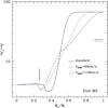 |
Fig. 6 Chemical profiles of carbon isotopic ratio as a function of coordinate in mass (Mr/M⊙) at the turn-off of the 1.5 M⊙ star computed with different initial rotation velocities. The black solid, red dashed, and blue dot-dashed lines represent standard models, models including rotation with VZAMS = 50 km s-1, and 110 km s-1, respectively. The vertical lines show, in all cases, the maximum depth reached by the convective envelope at its maximum extent during the first dredge-up, while the horizontal lines indicate the surface values of 12C/13C at the end of the first dredge-up. |
3.2. Evolution of lithium and isotopic ratio of carbon
We focus on the effects of rotation-induced mixing and thermohaline instability on Li and 12C/13C surface abundances. The best indicator of non-standard transport processes in evolved low-mass stars is the carbon isotopic ratio, as discussed in literature and supported by numerous observations (e.g. Gilroy 1989; Gratton et al. 2000; Smiljanic et al. 2009). The most fragile element, lithium, burns by proton capture at relatively low temperature (~2.5 × 10⁶ K) and is preserved only in the most external stellar layers (e.g. Pasquini et al. 2004; Charbonnel & Talon 1999; Palacios et al. 2003). Lithium and 12C/13C can be useful in the characterization of mixing mechanisms because they burn at different temperatures, i.e. at different depths in stellar interiors.
Figure 4 presents the evolutionary track in the Hertzsprung-Russell diagram of the 1.5 M⊙ model computed with thermohaline instability and rotation (VZAMS = 110 km s-1). We select two points along the track (turn-off and the bump luminosity) to discuss the evolution of the carbon isotopic ratio and lithium at the surface of low- and intermediate-mass stars.
Figure 5 represents the evolution of lithium and the isotopic ratio of carbon as a function of effective temperature for the same model. Standard predictions (i.e. non-rotating models without thermohaline mixing) are also shown.
In the standard case (solid line in Fig. 5), the surface depletion of both Li and 12C/13C begins at relatively low Teff (i.e. at Teff ~ 5600 K for Li and Teff ~ 5000 K for 12C/13C). This is due to the dilution of external layers when the convective stellar envelope deepens in mass during the first dredge-up. The surface abundances are not predicted to change after the end of the first dredge-up until the star reaches the early-AGB. In the next section we discuss the effects of rotation-induced mixing and thermohaline instability on the surface abundances of isotopic ratio of carbon and lithium.
3.2.1. At the turn-off
The modifications of the stellar internal and surface chemical abundances are driven by rotation-induced mixing on the main sequence and convective dilution during the first dredge-up episode on the subgiant branch and early-RGB. Figure 6 describes the effect of different initial velocities on the 12C/13C profile as a function of coordinate in mass1 (Mr/M⊙), at the end of central hydrogen burning in a 1.5 M⊙ model. In the rotating models, the abundance gradients are smoothed compared to the standard case. Rotation-induced mixing modifies the internal chemical structure of main-sequence stars, enlarging the Li-free regions and modifying the 13C and 12C profiles.
3.2.2. Toward the red giant branch
When the star expands after the turn-off (TO) and evolves toward the red giant branch, its convective envelope deepens and engulfs most of the regions that have been nuclearly processed as indicated by the vertical lines in Fig. 6. This leads to the first dredge-up, which changes the surface chemical properties of the star. Rotating subgiant stars have lower surface carbon isotopic ratio and lithium abundances compared to standard models (see Fig. 5, e.g., Palacios et al. 2003; Smiljanic et al. 2009). Indeed, when the initial velocity increases, the surface abundance of lithium after the first dredge-up decreases (see Fig. 7, at Teff ~ 4800 K). This implies that two stars with the same global properties (luminosity, surface gravity, or effective temperature) could have a very different surface abundance of lithium owing to their very different rotation velocities.
 |
Fig. 7 Evolution of the surface abundances of Lithium, A(Li), as a function of effective temperature. Predictions are shown for 2.0 M⊙ models at solar metallicity computed including rotation-induced mixing (VZAMS = 110, 180, 250 km s-1, black solid, green dashed, and red dotted lines, respectively) from the ZAMS up to the core-He-burning phase. ZAMS (black triangle) and first dredge-up (start/end; full/open squares) are indicated. |
 |
Fig. 8 Top panel: Kippenhahn diagram for the 1.5 M⊙ star computed with thermohaline instability and rotation-induced mixing. Here we focus on the red giant branch. Green dashed lines delimit the hydrogen-burning shell above the degenerate helium core, and the dotted line shows the region of maximum nuclear energy production. The region where thermohaline instability takes place is indicated in blue. Bottom panel: evolution of 12C/13C during the RGB. |
3.2.3. Red giant branch
The 12C/13C and Li abundances at the surface decrease during the RGB, and specifically at the bump luminosity, as shown by models including rotation-induced mixing and thermohaline instability (Figs. 4 and 5). As already discussed by Charbonnel & Zahn (2007) and CL10, on the RGB, thermohaline mixing becomes efficient close to the bump luminosity (Teff ~ 4200 K). Then, the theoretical abundances of Li and 12C/13C drop again (for more details see CL10), while they stay constant in the standard case.
Figure 8 displays a Kippenhahn diagram for a 1.5 M⊙ model as well as the evolution of the surface abundance of carbon isotopic ratio during the RGB. As discussed in Charbonnel & Zahn (2007) and CL10, thermohaline instability develops at the top of the hydrogen-burning shell (HBS) by an inversion of mean molecular weight. This instability is induced by the 3He(3He, 2p)4He reaction that takes place in the HBS, only after the star has reached the luminosity bump. This occurs when the HBS crosses the molecular weight discontinuity left behind by the first dredge-up (at t ~ 3.028 × 10⁹ yr in Fig. 8). As soon as the thermohaline instability sets in, newly emitted protons diffuse outward, spreading out the molecular-weight inversion and enlarging the thermohaline region until it reaches the convective envelope (at t ~ 3.039 × 10⁹ yr in Fig. 8). As a consequence, 12C and 13C diffuse respectively inward and outward, leading to a decrease in the surface carbon isotopic ratio. The surface Li abundance also decreases (Fig. 5). In addition, rotation-induced mixing leads to an earlier (in terms of luminosity) beginning of thermohaline instability on RGB compared to a model without rotation (see CL10).
3.2.4. He-burning phase
After the star reaches the RGB tip (at Teff ~ 3100 K), its effective temperature increases until it settles in the red clump (blue part in Fig. 5) before decreasing again when it starts climbing the asymptotic giant branch (AGB). During the core-He-burning phase, thermohaline instability develops and slightly changes the surface abundances of Li again and 12C/13C (see Fig. 5). The second dredge-up leads to another decrease in the Li abundance and, slightly, in 12C/13C. As shown by CL10, thermohaline mixing is responsible for the Li-enrichment shown during the thermal pulses AGB phase (TP-AGB), at Teff ~ 3000 K in Fig. 5 (red line). It can explain the Li-enrichment observed during the TP-AGB phase.
3.3. Variation of the asymptotic period spacing during stellar evolution
The period spacing of the dipolar gravity modes, ΔΠ(ℓ = 1), can be determined with the asymptotic relation (Tassoul 1980),  (5)where N is the Brunt-Väisälä frequency and r1 and r2 define the domain (in radius) where g modes are trapped. Within this region, the mode frequency satisfies the conditions
  (6)and
  (7)where Sl is the Lamb frequency and cs the sound velocity.
This quantity gives us information on the stellar structure and on the stellar core (Mosser et al. 2012b; Montalbán et al. 2013,L12a). Thus with the period spacing of g-modes, it is possible to distinguish between stars with the same luminosity but in different evolutionary phases. A difference in the density profile and the presence of a convective core during the core-He-burning phase change the value of ΔΠ(ℓ = 1). At the same luminosity, a RGB star has a lower ΔΠ(ℓ = 1) than a clump star (ΔΠ(ℓ = 1) ~60 and 300 s, respectively e.g. Mosser et al. 2014; Montalbán et al. 2010). Figure 9 depicts ΔΠ(ℓ = 1) for standard models of different initial stellar masses at solar metallicity. The density profile is different when the stellar mass increases, and, as a consequence, has an impact on the value ΔΠ(ℓ = 1) for a given evolutionary phase (see Fig. 9).
 |
Fig. 9 Stellar luminosity as a function of the asymptotic period spacing of g-modes for standard models at solar metallicity and for different stellar masses, as indicated. Subgiant and red giant phases are labelled by dashed and solid lines on the upper panel, which shows the red giant branch. The lower panel shows the He-burning phase. |
As we discuss in Sect. 3.2, rotation-induced mixing has an impact on the stellar structure during the main sequence, and leads to a more massive helium core at the turn-off than in the standard case. This results in a shift of tracks toward higher luminosities throughout their evolution (e.g. L12a, Eggenberger et al. 2010; Ekström et al. 2012; Maeder & Meynet 2000). The effect of increasing the mass of the He core at the TO is to change the time spent in the subgiant phase, as well as the period spacing (for stars with masses 2.0 M⊙) when the star will reach the phase of central He-burning (as explained in Montalban et al. 2013). Montalbán et al. (2013) already investigated the effect of main sequence overshooting on the period spacing of intermediate-mass stars during the core-He-burning, and also the effect of overshooting during the core-He-burning for low-mass stars. A detailed study of the impact of rotation is in progress (Lagarde et al., in prep.).
As discussed in Sect. 3.2, thermohaline mixing is efficient only after the bump luminosity on the RGB (Charbonnel & Zahn 2007; Charbonnel & Lagarde 2010). Beyond this point, the double-diffusive instability develops in a very thin region located between the hydrogen-burning shell and the convective envelope, and has a negligible effect on the stellar structure. It does not modify the tracks in the log (L) versus ΔΠ diagram.
4. Comparison with spectroscopic observations of CoRoT red giant targets
We now compare the theoretical predictions of our models with respect to observations of lithium and carbon isotopic ratio in red giant target.
 |
Fig. 10 Left panels: colour-coded Hertzsprung-Russell diagram for different stellar masses. The colour code represents the values of A(Li) at the stellar surface. Right panels: the evolution of surface lithium abundance (from the ZAMS to the end of the He-burning phase) as a function of effective temperature. Circles and diamonds denote, respectively, Li detections and upper limits for stars with [Fe/H] <−0.26 (top panels), −0.26 ≤ [Fe/H] <−0.125 (middle panels), and [Fe/H] ≥−0.125 (bottom panels). Error bars are shown for all stars. |
4.1. Lithium
Figure 10 presents theoretical lithium evolution for different masses, at three metallicities ([Fe/H] = −0.56, −0.25, and 0). The models include rotation with an initial velocity ~30% of critical velocity, which is typical of the observed rotation in the main-sequence stars in young open clusters (see Sect. 3, and L12). Theoretical tracks are compared to non-LTE Li observations in three metallicity ranges: [Fe/H] ≥ −0.125, −0.26 ≤ [ Fe/H ] < −0.125, and [Fe/H] < −0.26. Our sample does not include Li-rich giants with A(Li) > 2.5. The stellar surface gravity is taken from seismology for the stars observed by CoRoT. Otherwise we use stellar gravity deduced from spectroscopy.
In most cases, the theoretical and observed lithium abundances are compatible (within the error bars). However, a few cases should be discussed in detail:
-
HD 178484 (top panels of Fig. 10) has an observed surface lithium abundance A(Li) = 0.46 ± 0.12 higher than predicted by models (Fig. 10). As discussed by Smiljanic et al. (2010) and in Sect. 4, the lithium post-dredge-up abundance is dependent on the initial values of the stellar rotational velocities (see Fig. 7). If we were to adopt a lower initial value for the rotational velocity then better agreement would be seen between observation and theoretical models. This star could be a red giant star close to the bump luminosity with a low initial velocity.
-
For the same reason, the surface abundance of lithium in HD 45398 (middle panels of Fig. 10 with A(Li) = 0.63 ± 0.13, no seismic information) could be explained by a low initial velocity. We believe that this star is ascending the red giant branch.
-
Similarly to the two stars discussed before, HD 43023 (bottom panels of Fig. 10 with A(Li) < −0.16, no seismic information) is a red giant star beginning to climb the red giant branch, this time with a higher value of the initial velocity than the model shown because of the lower than expected lithium abundance.
-
HD 50890 (with A(Li) = 1.22, bottom panel of Fig. 10) has been studied by Baudin et al. (2012). They concluded, by modelling seismic properties, that it is a core He-burning star with mass in the range 3 to 5 M⊙. Its location in the log g − Teff diagram yields a similar stellar mass. However, owing to the large uncertainties on Li abundance, we cannot confirm the evolutionary status.
-
All members of NGC 6633 are discussed in detail in Sect. 4.3.
 |
Fig. 11 Theoretical evolutionary tracks plotted in log g − Teff diagram (from the main sequence up to the early-AGB) computed with thermohaline instability and rotation-induced mixing at solar metallicity (left panel) and at [Fe/H] = −0.56 (right panel). Different line styles correspond to different stellar masses. Position of the considered set of stars for which 12C/13C has been measured are represented by a circle for HD 175294, a square for HD 175679, a triangle for HD 181907, and a diamond for α Boo. They are segregated according to their metallicity. |
4.2. Carbon isotopic ratio
As discussed in Sect. 2, M14 investigated the carbon isotopic ratio in four stars. In this section, we discuss in detail these cases by comparing seismic and spectroscopic properties. In order to locate these stars on the evolutionary tracks, Fig. 11 presents the theoretical logg as a function of effective temperature for different masses and at two metallicities. In addition, the theoretical 12C/13C surface evolution with Teff for different stellar masses at two metallicities are shown in Fig. 12, and are compared with the observations.
These four stars present low carbon isotopic ratios that are not predicted by standard models. However, effects of rotation and, more significantly, thermohaline mixing can account for such a decrease in 12C/13C surface abundances and reproduce very nicely the spectroscopic observations. The stellar mass and metallicity have an impact on the effects of thermohaline instability and rotation-induced mixing on stellar surface abundances (for more details see Charbonnel & Lagarde 2010; and Lagarde & Charbonnel, in prep.).
 |
Fig. 12 12C/13C data in our red giant stars that are segregated according to their metallicity (left and right panels include respectively sample stars with metallicity close to solar and [Fe/H] = −0.56). Same symbols as in Fig. 11. Theoretical 12C/13C surface abundance is shown from the ZAMS up to the TP-AGB. Various lines correspond to predictions of stellar models of different masses including effects of rotation-induced mixing (with an initial VZAMS/Vcrit = 0.30) and thermohaline instability. |
The upper limits of Li abundances for HD 175294 (circle) and Arcturus (αBoo, diamond) do not give additional constraints, although they are consistent with their carbon isotopic ratio.
According to its low 12C/13C value (right panel of Fig. 12), Arcturus is an early-AGB star that has already finished the core He-burning phase, with a stellar mass between 1.0 and 1.25 M⊙. Its position on the evolutionary tracks (right panel Fig. 11) confirms its early-AGB status. The seismic properties were derived by Kallinger et al. (2010b). As shown by Miglio (2012), using the interferometric radius does not significantly change the stellar mass. Indeed, as shown in Fig. 2 and in Fig. 3 of Miglio (2012), the stellar mass of Arcturus is between 0.6 and 0.9 M⊙. The seismic mass is significantly below that inferred from the models. However, as Arcturus is believed to be an early-AGB, we can expect it to have experienced high mass loss. Indeed, using the Reimers formula in our models, we find that a star with an initial mass between 1.0 and 1.2 M⊙ at [Fe/H] = −0.56 has a mass between 0.9 and 1.17 M⊙ on the early-AGB.
HD 175294, was initially proposed as a potential target for CoRoT, but was not observed. Consequently, we have access only to the spectroscopic surface gravity which is more uncertain. From spectroscopic point of view, this star is likely to be a core-He-burning star with a stellar mass around 3.0 M⊙.
HD 175679 (square in Figs. 11 and 12) has seismic data with very large uncertainties that prevent an accurate estimation of seismic mass and radius. The Li abundance is in agreement with that of a star with a mass range of 3 to 4 M⊙ located in the Hertzsprung-gap or possibly at the base of the RGB. Although the carbon isotopic ratio is uncertain, the value is consistent with this evolutionary state and initial mass.
The properties of the red giant HD 181907 (HR 7349, triangle in Figs. 11 and 12) has been widely discussed in the literature. Using solely the seismic observations by Carrier et al. (2010), Miglio et al. (2010) deduce a mass of about 1.2 M⊙, which is in good agreement with the value we deduced from spectroscopic constraints (see Figs. 11 and 12), as well as with stellar mass and radius deduced from the Hipparcos parallax (Fig. 2).
An observation of the small frequency separation between ℓ = 0 and ℓ = 1 modes, δν01, allowed Montalbán et al. (2010) to suggest that this star is ascending or descending the RGB. However, the value of the small frequency separation between ℓ = 0 and ℓ = 2 modes, δν02, (Carrier et al. 2010) seems to be too large for a RGB star (Montalbán et al. 2012). In addition its low surface carbon isotopic ratio and Li abundances indicate that this star would be better explained by a model in the core-He-burning phase (Fig. 12).
Further seismic analysis can be used to distinguish between the RGB and core-He-burning phase. Measurement of the period spacing indicates that a value of around 285 s can fit the modes. This solution is not unique owing to the limited number of mixed modes observed with a five-month run. However, we can rule out a period spacing of about 60 s typical of an RGB star. We also applied the method of Kallinger et al. (2012) to estimate the evolutionary status, but again the frequency resolution makes it difficult to draw a firm conclusion. Further confirmation of the evolutionary state is derived from a comparison of the oscillation spectrum of HD 181907 with spectra of Kepler red giants with similar large separations and νmax values, and with identified evolutionary stages (Mosser et al. 2014). In that respect, the spectrum of HD 181907 looks like a red-clump star spectrum, with significant power in the gravity-dominated mixed modes (Grosjean et al. 2014). We therefore believe this star to be a core-He-burning star, based on both spectrometric and asteroseismic arguments. Nevertheless, it would be interesting to develop more detailed models of this star by computing theoretical oscillation frequencies directly from stellar models including the effects of, for example, thermohaline instability and rotation-induced mixing.
 |
Fig. 13 Theoretical evolutionary tracks plotted in log g − Teff diagram (left panel) and stellar radius (right panel) (from the main sequence up to the early-AGB) computed with thermohaline instability and rotation-induced mixing at solar metallicity for 4.0 M⊙ (VZAMS = 144 km s-1, solid black line), 3.0 M⊙ (VZAMS = 136 km s-1, orange long dashed line), 2.7 M⊙ (VZAMS = 110 km s-1, blue dashed line), and 2.5 M⊙ (VZAMS = 110 km s-1, red dashed line). Cluster members discussed in this study are indicated by green circle (HD 170231), square (HD 170174), and triangle (HD 170053). |
 |
Fig. 14 Theoretical evolution of lithium A(Li) (left panel) and the carbon isotopic ratio (right panel) as a function of effective temperature (from the main sequence up to the early-AGB) computed with thermohaline instability and rotation-induced mixing at solar metallicity for 4.0 M⊙ (VZAMS = 144 km s-1, solid black line), 2.7 M⊙ (VZAMS = 110 and 250 km s-1, blue and light blue dashed lines, respectively), and 2.5 M⊙ (VZAMS = 110 km s-1, red dashed line). The 4.0 M⊙ model following standard evolution theory is also indicated by dash-dotted line. Lithium detection and 12C/13C determination for cluster members are indicated by green symbols. |
4.3. NGC 6633
Since stars belonging to a cluster were formed together, we can assume that they have the same age, distance, and metallicity. Spectroscopic and asteroseismic data for these stars represent a unique opportunity to improve the constraints on mixing inside red giant stars. CoRoT has detected solar-like oscillations in three members of open cluster NGC 6633 (HD 170053, HD 170174, HD 170231; Barban et al. 2013; Poretti et al. 2015). In addition, M14 and Smiljanic et al. (2009) present spectroscopic studies of these stars. The lithium abundances are taken from M14 and the carbon isotopic ratio for two stars from Smiljanic et al. (2009). The age of the cluster determined by isochrone fitting in Smiljanic et al. (2009) (t = 4.5 × 10⁸ yrs) implies that stars in the He-core-burning stage have 2.8 ≲ M/M⊙ ≲ 3.0, which is compatible with the stellar mass determined with asteroseismology.
Although Molenda-Zakowicz et al. (2014) very recently presented a study of five stars in NGC 6811 observed by Kepler; NGC 6633 is the only cluster for which spectroscopic probes of extra-mixing on RGB (Li and 12C/13C) and asteroseismic properties are available. All spectroscopic and asteroseismic properties for members of NGC 6633 are listed in Table 2.
Figure 13 presents observations in log g − Teff diagram and stellar radius versus Teff. In the same figure, four evolutionary tracks for 2.5, 2.7, and 4.0 M⊙ at solar metallicity are shown. These tracks include the effects of rotation and thermohaline mixing. The turn-off mass of NGC 6633 lies in the range 2.4 to 2.7 M⊙ (Smiljanic et al. 2009).
Figure 14 presents chemical properties of the cluster members with lithium (left panel) and carbon isotopic ratio (right panel). Intermediate-mass stars ignite central helium-burning in a non-degenerate core and at relatively low luminosity on the RGB, well before the HBS reaches the mean molecular weight discontinuity caused by the first dredge-up. Consequently, thermohaline mixing does not take place in those stars. Only rotation has an impact on surface abundances (see right panel in Fig. 14).
In the following paragraphs, we discuss each star according to its seismic and spectroscopic properties.
-
HD 170053 (triangle in Figs. 13 and 14): according to its position in the colour-magnitude diagram and using isochrones from Schaller et al. (1992), Smiljanic et al. (2009) proposed that this star could be an early-AGB star. This is perfectly in agreement with the carbon isotopic ratio around 18 ± 8 that they deduced (see right panel of Fig. 14). As discussed in Sect. 3.2, rotation has an impact on stellar structure during the main sequence. This significantly changes the lithium profile at the end of the main sequence and the surface abundances in the subgiant phase (e.g. Palacios et al. 2003; Smiljanic et al. 2010). Taken together, log g, Teff, seismic radius, and the values of Li and 12C/13C suggest that this star is an early-AGB star with low initial velocity (see Fig. 7).
-
HD 170174 (square in Figs. 13 and 14): according to seismic properties this star has a stellar mass 2.7 ± 0.7 M⊙, which is slightly lower than the mass deduced from its position on the evolutionary tracks. Indeed, from a spectroscopic point of view, HD 170174 could be more massive (~3.0 M⊙) as a He-burning star with low initial velocity, or a red giant star at the bottom of RGB. Owing to the very short lifetime on the subgiant branch, the latter possibility is unlikely. Using the seismic stellar mass (2.7 M⊙) and considering this star as an He-burning star, the model with an initial velocity ~95 km s-1 at the ZAMS is the best model to reproduce its chemical properties.
-
HD 170231 (circle in Figs. 13 and 14): according to spectroscopic and seismic properties, this star could be a subgiant or a He-burning star. The low value of Δν rules out the possibility that this star is a subgiant. Its seismic properties give a stellar mass around 3.4 M⊙, which is in good agreement with its position on evolutionary tracks and its lithium abundance. A determination of the period spacing of g-modes would allow us to distinguish between these two evolutionary options.
5. Discussion and conclusions
In this paper, we demonstrate the power of the combination of seismic and spectroscopic constraints to improve our understanding of the physical processes and specifically extra-mixing taking place in the interior of red giant stars. Indeed, asteroseismology gives us new informations on stellar interiors and accurate estimates of stellar mass, radius, and evolutionary state. Spectroscopy provides complementary information about surface chemical properties of stars.
This paper significantly advances the study of CoRoT red giants as presented by M14 by adding a comparison with modern stellar models that incorporate rotation and thermohaline mixing. We compare stellar masses and radii determined using various methods. The estimates are in agreement within a standard uncertainty. However, we found relatively large average uncertainties on radii (~9%), and masses (~22%) due to large uncertainties on seismic properties (Δν or νmax). These values are dominated by the stars observed in short and initial CoRoT runs. These uncertainties are significantly lower when considering only stars observed in 150-day runs and with an apparent visual magnitude brighter than 8 (~5% on radius and ~14% on mass). These statistical uncertainties are likely to be larger than systematic uncertainties that may affect these relations.
The weighted average of the relative difference between Hipparcos and seismic distances (−0.12 ± 0.03) indicates a possible disagreement. However, the large uncertainty on these two quantities prevents us from drawing any firm conclusions.
We have also compared theoretical and observational behaviours for lithium and the carbon isotopic ratio. Stellar models used in this article include the effects of rotation-induced mixing (Zahn 1992; Maeder & Zahn 1998) known to change chemical properties of main sequence and subgiant stars, and thermohaline instability (Charbonnel & Zahn 2007; Charbonnel & Lagarde 2010) known to govern the surface chemical properties of low-mass RGB stars. We show that for low-mass stars like Arcturus and HD181907, the low carbon isotopic ratio is nicely explained by thermohaline instability. On the other hand, for more massive stars it is rotation that is the most efficient transport process for chemical species. Our models at different initial velocities can explain the surface abundances of lithium and 12C/13C.
Theoretical surface values of carbon isotopic ratio at the end of the first dredge-up and during the He-burning phase.
This study could be more quantitative if the seismic and spectroscopic constraints were more accurate. In addition, the small number of stars limits the conclusions. However, our study has identified the key constraints, and their precision, that are needed for a stringent test of our models. The desirable scenario is the following: to use asteroseismic and spectroscopic constraints to infer stellar masses to 10% or better, the evolutionary state (RGB versus. core-He-burning), and photospheric carbon isotopic ratio with an uncertainty of ±1. Table 3 presents the difference in the theoretical rotational velocity at the ZAMS needed to reproduce observations with these precisions. Thermohaline mixing governs the surface chemical properties of low-mass-RGB stars (M ≲ 1.5 M⊙) after the RGB bump. Whatever the rotational velocity at the ZAMS, the surface values of 12C/13C of a 1.25 M⊙ star during the He-burning phase are almost the same. As a consequence, ΔVZAMS is larger after the RGB than before thermohaline mixing occurs. The efficiency of thermohaline mixing decreases with increasing initial stellar mass (Charbonnel & Lagarde 2010; Lagarde et al. 2011). This is the reason why, for intermediate-mass stars, ΔVZAMS stays almost constant between the beginning of RGB and the He-burning phase. This ideal scenario may be achievable with data from the Kepler satellite which will yield a larger number of targets with precise seismic data. However, complementary spectroscopic data (e.g. Carlberg et al. 2015) with sufficient precision and accuracy will also be necessary.
We note, however, that a discrepancy still exists between the rotation profile deduced from asteroseismic observations (e.g. Beck et al. 2012; Mosser et al. 2012a) and the profiles predicted from models including shellular rotation and related meridional flows and turbulence (Eggenberger et al. 2012; Marques et al. 2013). The core rotation rate derived by asteroseimic observations are two orders of magnitude below the rotation rate predicted by theory. This implies the need for a powerful mechanism for extracting angular momentum from the core of red giant stars. More specific information about the stellar core like the period spacing of g-modes or the core rotation rate could help us to improve stellar models and physical processes occurring in red giant stars. The surface and core rotation rate as inferred from Kepler data will provide additional constraints.
With NGC 6633, we presented a first example of a cluster observed by CoRoT including RGB stars, for which chemical properties are also available. It is found that the distances for the cluster members deduced from asteroseismic properties are self consistent, but slightly large compared to Hipparcos distances. Although the stellar masses deduced from seismic properties present significant uncertainties, it is clear that the cluster members are in the mass range where rotation is the most efficient transport processes for chemical elements. Additional information of the rotation profile of these stars is needed to improve our understanding of red giant stars in this cluster.
The space mission Kepler and K2 have observed many more open clusters with different turnoff masses, which give us a unique opportunity to follow the evolution of stellar properties through the evolution, and to probe the role of transport processes at different evolutionary phases and different masses. For many of these stars we will be able to use period spacing and rotational splitting to determine evolutionary state and core rotation rate. To obtain the most information possible from the data set, the asteroseismic properties must be matched by the knowledge of the surface chemical abundances. We have shown in this paper how this complementary data set allows us to provide constraints on the physical processes in stellar interiors. In the future, the Gaia-ESO survey and APOGEE would be extremely helpful.
Mr/M⊙ allows us to point out the central regions of the star.
Acknowledgments
N.L. acknowledges financial support from Marie Curie Intra-European fellowship (FP7-PEOPLE-2012-IEF). T.M. acknowledges financial support from Belspo for contract PRODEX GAIA-DPAC. B.M., C.B., and E.M. acknowledge financial support from the Programme National de Physique Stellaire (CNRS/INSU) and from the ANR program IDEE Interaction Des Étoiles et des Exoplanètes. M.R. acknowledges financial support from the FP7 project SPACEINN: Exploitation of Space Data for Innovative Helio- and Asteroseismology. A.M., L.G., and E.P. acknowledge financial support from PRIN INAF-2014. The research leading to the presented results has received funding from the European Research Council under the European Community’s Seventh Framework Programme (FP7/2007−2013)/ERC grant agreement No. 338251 (StellarAges).
References
- Alonso, A., Arribas, S., & Martínez-Roger, C. 1999, A&AS, 140, 261 [NASA ADS] [CrossRef] [EDP Sciences] [Google Scholar]
- Angelou, G. C., Church, R. P., Stancliffe, R. J., Lattanzio, J. C., & Smith, G. H. 2011, ApJ, 728, 79 [NASA ADS] [CrossRef] [Google Scholar]
- Angelou, G. C., Stancliffe, R. J., Church, R. P., Lattanzio, J. C., & Smith, G. H. 2012, ApJ, 749, 128 [NASA ADS] [CrossRef] [Google Scholar]
- Baglin, A., Auvergne, M., Boisnard, L., et al. 2006, 36th COSPAR Scientific Assembly, 36, 3749 [Google Scholar]
- Barban, C., Baudin, F., Poretti, E., et al. 2013, in ASP Conf. Ser. 478, eds. K. Jain, S. C. Tripathy, F. Hill, J. W. Leibacher, & A. A. Pevtsov, 385 [Google Scholar]
- Baudin, F., Barban, C., Goupil, M. J., et al. 2012, A&A, 538, A73 [NASA ADS] [CrossRef] [EDP Sciences] [Google Scholar]
- Beck, P. G., Montalban, J., Kallinger, T., et al. 2012, Nature, 481, 55 [NASA ADS] [CrossRef] [Google Scholar]
- Bedding, T. R., Huber, D., Stello, D., et al. 2010, ApJ, 713, L176 [NASA ADS] [CrossRef] [Google Scholar]
- Borucki, W. J., Koch, D., Basri, G., et al. 2010, Science, 327, 977 [NASA ADS] [CrossRef] [PubMed] [Google Scholar]
- Brown, J. M., Garaud, P., & Stellmach, S. 2013, ApJ, 768, 34 [NASA ADS] [CrossRef] [Google Scholar]
- Carlberg, J. K., Smith, V. V., Cunha, K., et al. 2015, ApJ, 802, 7 [NASA ADS] [CrossRef] [Google Scholar]
- Carrier, F., De Ridder, J., Baudin, F., et al. 2010, A&A, 509, A73 [NASA ADS] [CrossRef] [EDP Sciences] [Google Scholar]
- Chaplin, W. J., & Miglio, A. 2013, ARA&A, 51, 353 [NASA ADS] [CrossRef] [Google Scholar]
- Chaplin, W. J., Elsworth, Y., Isaak, G. R., et al. 1998, MNRAS, 300, 1077 [NASA ADS] [CrossRef] [Google Scholar]
- Charbonnel, C. 1995, ApJ, 453, L41 [NASA ADS] [CrossRef] [Google Scholar]
- Charbonnel, C., & Lagarde, N. 2010, A&A, 522, A10 [NASA ADS] [CrossRef] [EDP Sciences] [MathSciNet] [PubMed] [Google Scholar]
- Charbonnel, C., & Talon, S. 1999, A&A, 351, 635 [NASA ADS] [Google Scholar]
- Charbonnel, C., & Talon, S. 2008, in IAU Symp. 252, eds. L. Deng, & K. L. Chan, 163 [Google Scholar]
- Charbonnel, C., & Zahn, J.-P. 2007, A&A, 467, L15 [NASA ADS] [CrossRef] [EDP Sciences] [Google Scholar]
- Charbonnel, C., Decressin, T., Amard, L., Palacios, A., & Talon, S. 2013, A&A, 554, A40 [NASA ADS] [CrossRef] [EDP Sciences] [Google Scholar]
- Cutri, R. M., Skrutskie, M. F., van Dyk, S., et al. 2003, 2MASS All Sky Catalog of point sources [Google Scholar]
- da Silva, L., Girardi, L., Pasquini, L., et al. 2006, A&A, 458, 609 [NASA ADS] [CrossRef] [EDP Sciences] [Google Scholar]
- Deheuvels, S., García, R. A., Chaplin, W. J., et al. 2012, ApJ, 756, 19 [NASA ADS] [CrossRef] [Google Scholar]
- Deheuvels, S., Doğan, G., Goupil, M. J., et al. 2014, A&A, 564, A27 [NASA ADS] [CrossRef] [EDP Sciences] [Google Scholar]
- Denissenkov, P. A. 2010, ApJ, 723, 563 [NASA ADS] [CrossRef] [Google Scholar]
- Denissenkov, P. A., & Merryfield, W. J. 2011, ApJ, 727, L8 [NASA ADS] [CrossRef] [Google Scholar]
- Denissenkov, P. A., & Tout, C. A. 2000, MNRAS, 316, 395 [NASA ADS] [CrossRef] [Google Scholar]
- Denissenkov, P. A., Pinsonneault, M., & MacGregor, K. B. 2009, ApJ, 696, 1823 [NASA ADS] [CrossRef] [Google Scholar]
- Drimmel, R., Cabrera-Lavers, A., & López-Corredoira, M. 2003, A&A, 409, 205 [NASA ADS] [CrossRef] [EDP Sciences] [Google Scholar]
- Eggenberger, P., Maeder, A., & Meynet, G. 2005, A&A, 440, L9 [NASA ADS] [CrossRef] [EDP Sciences] [Google Scholar]
- Eggenberger, P., Miglio, A., Montalban, J., et al. 2010, A&A, 509, A72 [NASA ADS] [CrossRef] [EDP Sciences] [Google Scholar]
- Eggenberger, P., Montalbán, J., & Miglio, A. 2012, A&A, 544, L4 [NASA ADS] [CrossRef] [EDP Sciences] [Google Scholar]
- Eggleton, P. P., Dearborn, D. S. P., & Lattanzio, J. C. 2006, Science, 314, 1580 [NASA ADS] [CrossRef] [PubMed] [Google Scholar]
- Eggleton, P. P., Dearborn, D. S. P., & Lattanzio, J. C. 2008, ApJ, 677, 581 [NASA ADS] [CrossRef] [Google Scholar]
- Ekström, S., Georgy, C., Eggenberger, P., et al. 2012, A&A, 537, A146 [NASA ADS] [CrossRef] [EDP Sciences] [Google Scholar]
- Gaigé, Y. 1993, A&A, 269, 267 [Google Scholar]
- Gilroy, K. K. 1989, ApJ, 347, 835 [NASA ADS] [CrossRef] [Google Scholar]
- Gilroy, K. K., & Brown, J. A. 1991, ApJ, 371, 578 [NASA ADS] [CrossRef] [Google Scholar]
- Gratton, R. G., Sneden, C., Carretta, E., & Bragaglia, A. 2000, A&A, 354, 169 [NASA ADS] [Google Scholar]
- Grosjean, M., Dupret, M.-A., Belkacem, K., et al. 2014, A&A, 572, A11 [NASA ADS] [CrossRef] [EDP Sciences] [Google Scholar]
- Hekker, S., Broomhall, A.-M., Chaplin, W. J., et al. 2010, MNRAS, 402, 2049 [NASA ADS] [CrossRef] [Google Scholar]
- Kallinger, T., Mosser, B., Hekker, S., et al. 2010a, A&A, 522, A1 [NASA ADS] [CrossRef] [EDP Sciences] [Google Scholar]
- Kallinger, T., Weiss, W. W., Barban, C., et al. 2010b, A&A, 509, A77 [NASA ADS] [CrossRef] [EDP Sciences] [Google Scholar]
- Kallinger, T., Hekker, S., Mosser, B., et al. 2012, A&A, 541, A51 [NASA ADS] [CrossRef] [EDP Sciences] [Google Scholar]
- Krishnamurti, R. 2003, J. Fluid Mech., 483, 287 [NASA ADS] [CrossRef] [Google Scholar]
- Lagarde, N., Charbonnel, C., Decressin, T., & Hagelberg, J. 2011, A&A, 536, A28 [NASA ADS] [CrossRef] [EDP Sciences] [Google Scholar]
- Lagarde, N., Decressin, T., Charbonnel, C., et al. 2012a, A&A, 543, A108 [NASA ADS] [CrossRef] [EDP Sciences] [Google Scholar]
- Lagarde, N., Romano, D., Charbonnel, C., et al. 2012b, A&A, 542, A62 [NASA ADS] [CrossRef] [EDP Sciences] [Google Scholar]
- Lattanzio, J. C., Siess, L., Church, R. P., et al. 2015, MNRAS, 446, 2673 [NASA ADS] [CrossRef] [Google Scholar]
- Maeder, A., & Meynet, G. 2000, ARA&A, 38, 143 [NASA ADS] [CrossRef] [Google Scholar]
- Maeder, A., & Zahn, J.-P. 1998, A&A, 334, 1000 [NASA ADS] [Google Scholar]
- Marques, J. P., Goupil, M. J., Lebreton, Y., et al. 2013, A&A, 549, A74 [NASA ADS] [CrossRef] [EDP Sciences] [Google Scholar]
- Melis, C., Reid, M. J., Mioduszewski, A. J., Stauffer, J. R., & Bower, G. C. 2014, Science, 345, 1029 [NASA ADS] [CrossRef] [PubMed] [Google Scholar]
- Miglio, A. 2012, Asteroseismology of Red Giants as a Tool for Studying Stellar Populations: First Steps, eds. A. Miglio, J. Montalbán, & A. Noels, 11 [Google Scholar]
- Miglio, A., Montalbán, J., Carrier, F., et al. 2010, A&A, 520, L6 [NASA ADS] [CrossRef] [EDP Sciences] [Google Scholar]
- Miglio, A., Brogaard, K., Stello, D., et al. 2012, MNRAS, 419, 2077 [NASA ADS] [CrossRef] [Google Scholar]
- Molenda-Zakowicz, J., Brogaard, K., Niemczura, E., et al. 2014, MNRAS, 445, 2446 [NASA ADS] [CrossRef] [Google Scholar]
- Montalbán, J., Miglio, A., Noels, A., Scuflaire, R., & Ventura, P. 2010, ApJ, 721, L182 [NASA ADS] [CrossRef] [Google Scholar]
- Montalbán, J., Miglio, A., Noels, A., et al. 2012, Adiabatic Solar-Like Oscillations in Red Giant Stars, eds. A. Miglio, J. Montalbán, & A. Noels, 23 [Google Scholar]
- Montalbán, J., Miglio, A., Noels, A., et al. 2013, ApJ, 766, 118 [NASA ADS] [CrossRef] [Google Scholar]
- Morel, T., Miglio, A., Lagarde, N., et al. 2014, A&A, 564, A119 [NASA ADS] [CrossRef] [EDP Sciences] [Google Scholar]
- Mosser, B., & Appourchaux, T. 2009, A&A, 508, 877 [NASA ADS] [CrossRef] [EDP Sciences] [Google Scholar]
- Mosser, B., Barban, C., Montalbán, J., et al. 2011, A&A, 532, A86 [NASA ADS] [CrossRef] [EDP Sciences] [Google Scholar]
- Mosser, B., Goupil, M. J., Belkacem, K., et al. 2012a, A&A, 548, A10 [NASA ADS] [CrossRef] [EDP Sciences] [Google Scholar]
- Mosser, B., Goupil, M. J., Belkacem, K., et al. 2012b, A&A, 540, A143 [NASA ADS] [CrossRef] [EDP Sciences] [Google Scholar]
- Mosser, B., Michel, E., Belkacem, K., et al. 2013, A&A, 550, A126 [NASA ADS] [CrossRef] [EDP Sciences] [Google Scholar]
- Mosser, B., Benomar, O., Belkacem, K., et al. 2014, A&A, 572, L5 [NASA ADS] [CrossRef] [EDP Sciences] [PubMed] [Google Scholar]
- Palacios, A., Talon, S., Charbonnel, C., & Forestini, M. 2003, A&A, 399, 603 [NASA ADS] [CrossRef] [EDP Sciences] [Google Scholar]
- Palacios, A., Charbonnel, C., Talon, S., & Siess, L. 2006, A&A, 453, 261 [NASA ADS] [CrossRef] [EDP Sciences] [Google Scholar]
- Pasquini, L., Bonifacio, P., Randich, S., Galli, D., & Gratton, R. G. 2004, A&A, 426, 651 [NASA ADS] [CrossRef] [EDP Sciences] [Google Scholar]
- Poretti, E., Mathias, P., Barban, C., et al. 2015, Astrophys. Space Sci. Proc., 39, 101 [NASA ADS] [CrossRef] [Google Scholar]
- Rodrigues, T. S., Girardi, L., Miglio, A., et al. 2014, MNRAS, 445, 2758 [NASA ADS] [CrossRef] [Google Scholar]
- Rosenblum, E., Garaud, P., Traxler, A., & Stellmach, S. 2011, ApJ, 731, 66 [NASA ADS] [CrossRef] [Google Scholar]
- Schaller, G., Schaerer, D., Meynet, G., & Maeder, A. 1992, A&AS, 96, 269 [Google Scholar]
- Smiljanic, R., Gauderon, R., North, P., et al. 2009, A&A, 502, 267 [NASA ADS] [CrossRef] [EDP Sciences] [Google Scholar]
- Smiljanic, R., Pasquini, L., Charbonnel, C., & Lagarde, N. 2010, A&A, 510, A50 [NASA ADS] [CrossRef] [EDP Sciences] [Google Scholar]
- Sweigart, A. V., & Mengel, J. G. 1979, ApJ, 229, 624 [NASA ADS] [CrossRef] [Google Scholar]
- Talon, S., & Charbonnel, C. 1998, A&A, 335, 959 [NASA ADS] [Google Scholar]
- Talon, S., & Charbonnel, C. 2005, A&A, 440, 981 [NASA ADS] [CrossRef] [EDP Sciences] [Google Scholar]
- Tassoul, M. 1980, ApJS, 43, 469 [NASA ADS] [CrossRef] [Google Scholar]
- Tautvaišiene, G., Edvardsson, B., Tuominen, I., & Ilyin, I. 2000, A&A, 360, 499 [NASA ADS] [Google Scholar]
- Tautvaišienė, G., Barisevičius, G., Chorniy, Y., Ilyin, I., & Puzeras, E. 2013, MNRAS, 430, 621 [NASA ADS] [CrossRef] [Google Scholar]
- Thygesen, A. O., Frandsen, S., Bruntt, H., et al. 2012, A&A, 543, A160 [NASA ADS] [CrossRef] [EDP Sciences] [Google Scholar]
- Traxler, A., Garaud, P., & Stellmach, S. 2011, ApJ, 728, L29 [NASA ADS] [CrossRef] [Google Scholar]
- Ulrich, R. K. 1972, ApJ, 172, 165 [NASA ADS] [CrossRef] [Google Scholar]
- van Leeuwen, F. 2007, Hipparcos, the New Reduction of the Raw Data, Astrophys. Space Sci. Lib., 350, [Google Scholar]
- van Leeuwen, F. 2009, A&A, 497, 209 [NASA ADS] [CrossRef] [EDP Sciences] [Google Scholar]
- Wachlin, F. C., Vauclair, S., & Althaus, L. G. 2014, A&A, 570, A58 [NASA ADS] [CrossRef] [EDP Sciences] [Google Scholar]
- Zahn, J.-P. 1992, A&A, 265, 115 [NASA ADS] [Google Scholar]
All Tables
Theoretical surface values of carbon isotopic ratio at the end of the first dredge-up and during the He-burning phase.
All Figures
|
Fig. 1 Comparison between the radii obtained by different combinations of the available observational constraints. Radii are determined using asteroseismic constraints (νmax,Δν) and Teff (black dots); determined with PARAM (blue crosses); and using the parallax from the Hipparcos catalogue (van Leeuwen 2007), apparent magnitudes, and extinction from different prescriptions (red symbols). Squares represent radii computed with no extinction (AV = 0), and triangles extinctions from the 3D Galactic extinction model by Drimmel et al. (2003). Asterisks indicate stars that are members of NGC 6633. |
| In the text | |
|
Fig. 2 Comparison between the masses obtained by different combinations of the observational constraints available. Masses are determined using asteroseismic constraints (νmax,Δν) and Teff (black dots); using νmax, Teff, the extinction from Drimmel’s model, and the stellar radius from the Hipparcos parallax (using Teff, red triangles); and using Δν and the stellar radius from the Hipparcos parallax (using Teff) and stellar extinction by Drimmel’s model (green squares). Asterisks indicate stars that are members of NGC 6633. |
| In the text | |
|
Fig. 3 Comparison between the distances determined from asteroseismic constraints (νmax,Δν) and Teff (black dots), and the Hipparcos distance (red triangles). In the lower panel, the grey solid line represents the weighted average difference, while the grey dashed lines represent a difference of 25%. Asterisks identify the cluster members. |
| In the text | |
|
Fig. 4 Hertzsprung-Russell diagram of model with M = 1.5 M⊙ and solar metallicity including the effects of rotation-induced mixing and thermohaline instability. The colour represents the mass fraction of 12C/13C at the surface. The turn-off and the bump luminosity are indicated. |
| In the text | |
|
Fig. 5 Evolution of the lithium surface abundances (A(Li) = log( |
| In the text | |
|
Fig. 6 Chemical profiles of carbon isotopic ratio as a function of coordinate in mass (Mr/M⊙) at the turn-off of the 1.5 M⊙ star computed with different initial rotation velocities. The black solid, red dashed, and blue dot-dashed lines represent standard models, models including rotation with VZAMS = 50 km s-1, and 110 km s-1, respectively. The vertical lines show, in all cases, the maximum depth reached by the convective envelope at its maximum extent during the first dredge-up, while the horizontal lines indicate the surface values of 12C/13C at the end of the first dredge-up. |
| In the text | |
|
Fig. 7 Evolution of the surface abundances of Lithium, A(Li), as a function of effective temperature. Predictions are shown for 2.0 M⊙ models at solar metallicity computed including rotation-induced mixing (VZAMS = 110, 180, 250 km s-1, black solid, green dashed, and red dotted lines, respectively) from the ZAMS up to the core-He-burning phase. ZAMS (black triangle) and first dredge-up (start/end; full/open squares) are indicated. |
| In the text | |
|
Fig. 8 Top panel: Kippenhahn diagram for the 1.5 M⊙ star computed with thermohaline instability and rotation-induced mixing. Here we focus on the red giant branch. Green dashed lines delimit the hydrogen-burning shell above the degenerate helium core, and the dotted line shows the region of maximum nuclear energy production. The region where thermohaline instability takes place is indicated in blue. Bottom panel: evolution of 12C/13C during the RGB. |
| In the text | |
|
Fig. 9 Stellar luminosity as a function of the asymptotic period spacing of g-modes for standard models at solar metallicity and for different stellar masses, as indicated. Subgiant and red giant phases are labelled by dashed and solid lines on the upper panel, which shows the red giant branch. The lower panel shows the He-burning phase. |
| In the text | |
|
Fig. 10 Left panels: colour-coded Hertzsprung-Russell diagram for different stellar masses. The colour code represents the values of A(Li) at the stellar surface. Right panels: the evolution of surface lithium abundance (from the ZAMS to the end of the He-burning phase) as a function of effective temperature. Circles and diamonds denote, respectively, Li detections and upper limits for stars with [Fe/H] <−0.26 (top panels), −0.26 ≤ [Fe/H] <−0.125 (middle panels), and [Fe/H] ≥−0.125 (bottom panels). Error bars are shown for all stars. |
| In the text | |
|
Fig. 11 Theoretical evolutionary tracks plotted in log g − Teff diagram (from the main sequence up to the early-AGB) computed with thermohaline instability and rotation-induced mixing at solar metallicity (left panel) and at [Fe/H] = −0.56 (right panel). Different line styles correspond to different stellar masses. Position of the considered set of stars for which 12C/13C has been measured are represented by a circle for HD 175294, a square for HD 175679, a triangle for HD 181907, and a diamond for α Boo. They are segregated according to their metallicity. |
| In the text | |
|
Fig. 12 12C/13C data in our red giant stars that are segregated according to their metallicity (left and right panels include respectively sample stars with metallicity close to solar and [Fe/H] = −0.56). Same symbols as in Fig. 11. Theoretical 12C/13C surface abundance is shown from the ZAMS up to the TP-AGB. Various lines correspond to predictions of stellar models of different masses including effects of rotation-induced mixing (with an initial VZAMS/Vcrit = 0.30) and thermohaline instability. |
| In the text | |
|
Fig. 13 Theoretical evolutionary tracks plotted in log g − Teff diagram (left panel) and stellar radius (right panel) (from the main sequence up to the early-AGB) computed with thermohaline instability and rotation-induced mixing at solar metallicity for 4.0 M⊙ (VZAMS = 144 km s-1, solid black line), 3.0 M⊙ (VZAMS = 136 km s-1, orange long dashed line), 2.7 M⊙ (VZAMS = 110 km s-1, blue dashed line), and 2.5 M⊙ (VZAMS = 110 km s-1, red dashed line). Cluster members discussed in this study are indicated by green circle (HD 170231), square (HD 170174), and triangle (HD 170053). |
| In the text | |
|
Fig. 14 Theoretical evolution of lithium A(Li) (left panel) and the carbon isotopic ratio (right panel) as a function of effective temperature (from the main sequence up to the early-AGB) computed with thermohaline instability and rotation-induced mixing at solar metallicity for 4.0 M⊙ (VZAMS = 144 km s-1, solid black line), 2.7 M⊙ (VZAMS = 110 and 250 km s-1, blue and light blue dashed lines, respectively), and 2.5 M⊙ (VZAMS = 110 km s-1, red dashed line). The 4.0 M⊙ model following standard evolution theory is also indicated by dash-dotted line. Lithium detection and 12C/13C determination for cluster members are indicated by green symbols. |
| In the text | |
Current usage metrics show cumulative count of Article Views (full-text article views including HTML views, PDF and ePub downloads, according to the available data) and Abstracts Views on Vision4Press platform.
Data correspond to usage on the plateform after 2015. The current usage metrics is available 48-96 hours after online publication and is updated daily on week days.
Initial download of the metrics may take a while.