| Issue |
A&A
Volume 580, August 2015
|
|
|---|---|---|
| Article Number | A68 | |
| Number of page(s) | 15 | |
| Section | Interstellar and circumstellar matter | |
| DOI | https://doi.org/10.1051/0004-6361/201525669 | |
| Published online | 03 August 2015 | |
Temperatures of dust and gas in S 140⋆,⋆⋆
1 SRON Netherlands Institute for Space Research, Landleven 12, and Kapteyn Institute, University of Groningen, 9747 AD Groningen The Netherlands
e-mail: This email address is being protected from spambots. You need JavaScript enabled to view it.
2 Astronomy Department, University of Texas at Austin, 1 University Station C1400, Austin, TX 78712−0259, USA
e-mail: This email address is being protected from spambots. You need JavaScript enabled to view it.
3 I. Physikalisches Institut der Universität zu Köln, Zülpicher Strae 77, 50937 Köln, Germany
4 Department of Astronomy and Astrophysics, Tata Institute of Fundamental Research, Homi Bhabha Road, Colaba, 400005 Mumbai, India
5 Observatorio Astronómico Nacional (OAN, IGN), Apdo 112, 28803 Alcalá de Henares, Spain
6 Instituto Radioastronomía Milimétrica, Av. Divina Pastora 7, Nucleo Central, 18012 Granada, Spain
Received: 15 January 2015
Accepted: 13 May 2015
Abstract
Context. In dense parts of interstellar clouds (≥105 cm-3), dust and gas are expected to be in thermal equilibrium, being coupled via collisions. However, previous studies have shown that in the presence of intense radiation fields, the temperatures of the dust and gas may remain decoupled even at higher densities.
Aims. The objective of this work is to study in detail the temperatures of dust and gas in the photon-dominated region S 140, especially around the deeply embedded infrared sources IRS 1−3 and at the ionization front.
Methods. We derive the dust temperature and column density by combining Herschel-PACS continuum observations with SOFIA observations at 37 μm and SCUBA data at 450 μm. We model these observations using simple greybody fits and the DUSTY radiative transfer code. For the gas analysis we use RADEX to model the CO 1−0, CO 2−1, 13CO 1−0 and C18O 1−0 emission lines mapped with the IRAM-30 m telescope over a 4′ field. Around IRS 1−3, we use HIFI observations of single-points and cuts in CO 9−8, 13CO 10−9 and C18O 9−8 to constrain the amount of warm gas, using the best fitting dust model derived with DUSTY as input to the non–local radiative transfer model RATRAN. The velocity information in the lines allows us to separate the quiescent component from outflows when deriving the gas temperature and column density.
Results. We find that the gas temperature around the infrared sources varies between ~35 and ~55 K. In contrast to expectation, the gas is systematically warmer than the dust by ~5−15 K despite the high gas density. In addition we observe an increase of the gas temperature from 30−35 K in the surrounding up to 40−45 K towards the ionization front, most likely due to the UV radiation from the external star. Furthermore, detailed models of the temperature structure close to IRS 1 which take the known density gradient into account show that the gas is warmer and/or denser than what we model. Finally, modelling of the dust emission from the sub–mm peak SMM 1 constrains its luminosity to a few ×102L⊙.
Conclusions. We conclude that the gas heating in the S 140 region is very efficient even at high densities. The most likely explanation is deep UV penetration from the embedded sources in a clumpy medium and/or oblique shocks.
Key words: ISM: individual objects: S 140 / ISM: molecules / ISM: kinematics and dynamics / photon-dominated region (PDR) / radiative transfer / stars: formation
Based on Herschel observations. Herschel is an ESA space observatory with science instruments provided by European-led Principal Investigator consortia and with important participation from NASA.
Final Herschel and IRAM data (cube) as FITS files are only available at the CDS via anonymous ftp to cdsarc.u-strasbg.fr (130.79.128.5) or via http://cdsarc.u-strasbg.fr/viz-bin/qcat?J/A+A/580/A68
© ESO, 2015
1. Introduction
Stars are born inside dense molecular structures in the interstellar medium (ISM) that consist of gas and dust. The dust grains in clouds associated with star-forming regions absorb the short–wavelength radiation from the central stars, heat up, and then re-emit radiation at far-IR and sub–millimeter wavelengths. The thermal radiation from dust is optically thin at these wavelengths and thus is a good tracer of such physical parameters as temperature, density, and the gas mass of the clouds. Dust is efficiently heated through near IR radiation thanks to the broadband absorption properties of the dust grains. On the other hand, the gas temperature Tgas is mainly governed by heating processes driven by UV radiation (photoelectric heating, H2 excitation, dissociation).
In the well-shielded centers of massive cores, the primary effects for the thermal balance are cosmic ray heating, molecular line cooling, and collisional heating or cooling due to dust-gas collisions (Goldsmith & Langer 1978; Tielens 2005; Draine 2011).
At densities above ~104.5, the dust and gas are expected to be collisionally coupled and are characterized by the same temperature (Goldsmith 2001). At lower densities, the rate of collisions between dust and gas decreases, and the cooling of the gas via fine-structure and molecular rotational transitions becomes dominant (e.g. CO, [C II] , and [OI]; Sternberg & Dalgarno 1995; Kaufman et al. 1999; Meijerink & Spaans 2005).
Excitation of the rotational levels of molecules like CO (low dipole moment) observed at (sub)mm wavelengths is provided by collisions with H2. If these collisions are frequent enough to exceed the spontaneous decay rate, the levels will get into thermal equilibrium with H2. The critical densities ncr of CO and isotopologues for the J = 1 − 0 and 2−1 transitions at 50 K are ~ 2 × 103 cm-3 and ~ 2 × 104 cm-3, respectively1. At this point their excitation temperature will approach the gas kinetic temperature, so that the study of these lines is ideal for gas kinetic temperature estimates. The rarer isotopologues of CO, such as 13CO and C18O, can be used to probe regions of high column density where the lines of the abundant isotopologues become optically thick. The critical densities ncr of CO and isotopologues at 50 K are ~1.2 × 106 cm-3 for the J = 9 − 8 and ~ 1.5 × 106 cm-3 for the 10−9 transition, respectively.
S 140 is a well studied HII region that lies at the southwest edge of the molecular cloud L 1204 at a distance of 746 pc (Hirota et al. 2008). A larger distance of 910 pc has been adopted in previous studies (e.g., Crampton & Fisher 1974; Dedes et al. 2010; Ikeda & Kitamura 2011). This edge is illuminated by the B0V star HD 211880, creating a visible HII region and a photon-dominated region (PDR) at the ionization front (IF). The cloud also hosts a cluster of embedded high-mass young stellar objects (YSOs), IRS 1 to 3 (Evans et al. 1989) at a projected distance of ~ 75′′ northeast of the IF. A large number of low-mass stars are also forming, making S 140 an ideal laboratory for studying both the star formation of various masses and the differences caused by irradiation from external (B0V star) and internal sources (IRS 1 to 3).
The analysis of physical models around IRS 1 has been performed by a number of previous authors including Harvey et al. (1978), Gürtler et al. (1991), Minchin et al. (1993), van der Tak et al. (2000), Mueller et al. (2002), de Wit et al. (2009), and Maud & Hoare (2013). Poelman & Spaans (2006) report the clumpiness towards S 140 and give a value of nH2 ~ 104 cm-3 for the interclump medium and ~4 × 10⁵ for the clump gas. Previous models lacked spatial information at many wavelengths, and many of them were based on the assumption that the gas temperature is coupled to the dust as a result of the high densities (e.g., Poelman & Spaans 2006).
In this study we have analyzed the temperature and column density around the S 140 high-mass star–forming region of embedded young stellar objects by combining Herschel-PACS and HIFI data with ground-based mapping observations of mm–wave lines using the IRAM 30 m telescope. The new PACS continuum data and IRAM spectroscopic maps provide us with the highest angular resolution spatial information available, covering an area that includes the YSOs in both datasets. The IF was covered by our larger IRAM maps (4′× 4′) but not by the PACS observations, since the latter cover a smaller area (45′′× 45′′). Furthermore, the data give us the opportunity to study independently of the gas and dust temperatures around FIRS 1−3 and check whether the assumption of well-coupled dust and gas is valid throughout this cloud.
In the following sections, we present the dust and gas modeling, along with the resulting parameters. We present the observations in Sect. 2, the observational results in Sect. 3, the gas and dust analysis with a comparison between gas and dust in Sect. 4, the effect of density gradients using more advanced dust and gas models in Sect. 5, and a discussion of our results and conclusions in Sect. 6.
2. Observations and data reduction
2.1. PACS data
To investigate the temperature and column-density structure of the dust we analyzed a single footprint of PACS (Poglitsch et al. 2010) with its 5 × 5 spatial array of ~ 9′′ pixels over a range of wavelengths from ~ 70 μm to ~ 200 μm (obsId: 1342222256). The data was reduced using HIPE 9.1.
Since the PACS spectrometer continuum data only cover the peak of the spectral energy distribution (SED) for S 140, we have supplemented our analysis with shorter and longer wavelength images. We used the SOFIA/FORCAST images at 11.1, 31.5, and 37 μm discussed by Harvey et al. (2012) and the 24.5 μm Subaru/COMICS data of de Wit et al. (2009). Since all of these observations were obtained with resolution better than that of the PACS/Spec images, we used them both at their native resolution and reconvolved to the PACS/Spec 187 μm resolution. These raw and convolved images were also resampled to a 1′′ grid like the PACS/Spec images. Longward of the PACS wavelengths, the highest resolution image available is in the JCMT SCUBA archive2 at 450 μm. We have used this image without further processing in our analysis below. We also examined the SCUBA 850 μm image, which is qualitatively similar but has lower spatial resolution.
2.2. IRAM data
The 30 m observations were conducted during four hours on September 24, 2011. The Eight MIxer Receiver (EMIR) was used during the observations. CO J = 1 → 0 and isotopologues (~110−115 GHz, 3 mm) and CO J = 2 → 1 (230.54 GHz, 1 mm) map data were gathered in two linear polarizations. Our 4′× 4′ maps were centered close to S 140-IRS 1 position at RA = 22:19:18.30, Dec = 63:18:54.2 (J2000) (Fig. 2). For this work, we selected the maps of CO J = 1 → 0 (115.27 GHz), J = 2 → 1 (230.54 GHz), together with the isotopologues 13CO J = 1 → 0 (110.20 GHz) and C18O J = 1 → 0 (109.78 GHz). At all the observed lines, the FTS and WILMA were connected in parallel as backends. In the 3 mm set up, we collected data from three bands of ~ 4 GHz each including the isotopic lines of 13CO J = 1 → 0 and C18O J = 1 → 0 in the CO setup. The beam sizes are ~ 21′′ at 3 mm and ~ 11′′ at 1 mm.
The sky opacity measured by the taumeter at 225 GHz was stable at τ225 = − 0.26. Pointing and focus were checked about every hour on quasars and on Uranus and were stable within 2″ and 0.2 mm. The spectral line calibration was checked by pointed observations on IRS 1 and IF. The on–the–fly mapping observations were done in perpendicular directions to avoid scanning artifacts. The typical system temperatures were 96−215 K at 3 mm and 175−190 K at 1 mm. The resulting root mean square (rms) falls between 0.152−0.705 K at 3 mm and ~0.525 K at 1 mm for a velocity resolution of ~0.5 km s-1 and ~0.25 km s-1 respectively.
The intensities were converted from antenna temperature units to a scale of main-beam temperature (Tmb), dividing by the main-beam efficiencies ηmb (Beff/Feff) of 0.82 at 3 mm and 0.64 at 1 mm. Velocities are given with respect to the LSR. Baselines of orders 0 to 4 have been subtracted. Data reduction and analysis were performed using the GILDAS software3.
2.3. HIFI data
To test the reliability of our method for the gas analysis, we used single-pointing observations (spectra, Fig. 6) and cuts from Herschel-HIFI (Fig. 2, top), in addition to the 4′ × 4′ maps from IRAM-30 m. Single-pointing, frequency-switching spectra in bands 1a, 1b, 2b, 3a, 4a, 4b, 6b, and 7b and OTF maps were analyzed. The single-pointing data were taken toward S 140-IRS 1 at RA = 22:19:18.21, Dec = 63:18:46.9 (J2000) and toward a position in the IF at RA = 22:19:11.53, Dec = 63:17:46.9 (J2000).
For this analysis, we used only the observations of CO J = 9 → 8 (1036.9 GHz), together with the isotopologues, 13CO J = 10 → 9 (1101.35 GHz), C18O J = 9 → 8 (987.56 GHz), toward IRS 1 and IF (obsIds: 1342195050, 1342196426, 1342219209, 1342195049, 1342201741). In addition, we used the cuts of CO 9 → 8 and 13CO J = 10 → 9 (obsIds: 1342201741, 1342201806). The observed line parameters in units of antenna temperatures were corrected in units of main beam temperatures using the main beam efficiency of 0.74 (987.56 GHz, 1036.9 GHz, 1101.35 GHz) (Roelfsema et al. 2012), while the beam size at these frequencies is ~ 21′′.
3. Observational results
3.1. Dust continuum observations
For this analysis we selected our 45′′× 45′′ maps in a number of continuum wavelengths with no obvious line emission or with line emission that was easily masked. The particular wavelengths chosen were centered on the wavelengths for which convolution kernels have been developed by Aniano et al. (2011), which enabled us to convolve all maps to a common resolution. These wavelength PACS/Spec data are 73, 75, 84, 94, 110, 125, 136, 145, 150, 168, and 187 μm. We extracted 3% bandwidth continuum fluxes centered on each of these wavelengths while masking out obvious line emission. For comparison with other wavelength data, as well as for comparison with modeling results, we sampled all these images again to a 1′′ spatial grid (Fig. 1). For the final comparison the model images were convolved to a telescope point spread function, and typically a 9′′ square pixel was used to simulate the PACS/Spec observations.
Figure 1 shows the image at 73 μm. The 37 μm (SOFIA) emission is overlaid using black contours showing the positions of IRS 1, 2, and 3. As shown in the image, the emission from IRS 1 dominates at this wavelength.
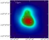 |
Fig. 1 PACS/Spec continuum image at 73 μm: 5 × 5 spatial array of 9′′ pixels resampled to 1′′ grid with contours of 37 μm (SOFIA) emission overlaid showing the positions of IRS 1, 2, and 3. |
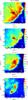 |
Fig. 2 Spatial distribution of CO 1−0, CO 2−1, 13CO 1−0, and C18O 1−0 peak intensities (HIFI cut and PACS overplotted). The IRS 1−3 positions were taken from Evans et al. (1989) & SMM 1 from Maud et al. (2013). The center is at RA = 22:19:18.30, Dec = 63:18:54.2 (J2000). |
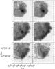 |
Fig. 3 Channel maps of CO 1−0 obtained with IRAM with the central velocities given in km s-1. The levels of contours are 45 K (darker) until 10 K (lighter) using steps of 5 K. |
Line parameters of CO and isotopologues toward the IRS 1 and IF positions – IRAM and HIFI data.
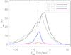 |
Fig. 4 Line profiles of CO 1−0 (black line), CO 2−1 (gray line), 13CO 1−0 (blue line), and C18O 1−0 (red line) toward IRS 1 as observed with IRAM (offset position: 0′′, –4.0′′). Wings are visible at blueshifted velocities. The dashed vertical line represents the velocity of the source (–7.1 km s-1). |
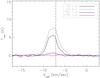 |
Fig. 5 Line profiles of CO 1−0 (black line), CO 2−1 (gray line), 13CO 1−0 (blue line), and C18O 1−0 (red line) toward the IF as observed with IRAM (offset position: –42.7′′, –68.0′′). The dashed vertical line represents the velocity of the source (–7.1 km s-1). |
3.2. The spatial and velocity distribution of CO emission
Figure 2 shows the maps of the peak intensities as observed in their original angular resolution at their peak velocities of CO 1−0, CO 2−1, 13CO 1−0, and C18O 1−0. The lines of the main isotope show two clearly disjointed peaks, one at the densest cluster between the YSOs IRS 1 and IRS 3, and one marking the external interface of the cloud illuminated by HD 211880. Because 13CO and C18O trace the column density structure, the interface peak is shifted into the cloud for these lines, merging with the peak around the embedded cluster.
Finally, while CO 1−0 and CO 2−1 peak toward IRS 1−3 (ΔRA: 10.70′′, ΔDec: –4.0′′), the 13CO 1−0 and C18O 1−0 peak closer to IRS 2 (ΔRA: –11.20′′, ΔDec: 18.30′′). C18O 1−0 shows a second peak southeast of IRS 1. This reflects a column density effect that is also revealed later in the column density map (see Fig. 11).
Figure 3 shows channel maps of CO 1−0 to illustrate the velocity structure. We find a clear velocity offset between the gas around the cluster and the interface and a much narrower velocity distribution of the interface gas. Figures 4−5 show the line profiles of CO and isotopologues as observed toward IRS 1 and IF. The peak velocity of the emission changes with position on the map. The IF peaks close to the velocity of the source that is ~ −7.1 km s-1, while IRS 1 peaks at ~ −3.6 km s-1. The difference may be caused by outflows driven by the infrared sources. For the above reasons we chose to model the peak intensities of the lines in their peak velocities.
3.3. Line profiles
The line profiles as shown in Figs. 4 and 5, are stronger toward IRS 1 and weaker toward the IF (Table 1). At the individual positions, the lines from CO are broader than the lines from the other isotopologues of CO (Figs. 4 and 6).
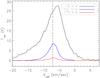 |
Fig. 6 Line profiles of CO 9−8 (black line), 13CO 10−9 (blue line), and C18O 9−8 (red line) toward IRS 1 as observed with HIFI (RA = 22:19:18.21, Dec = 63:18:46.9). The dashed vertical line represents the velocity of the source (–7.1 km s-1). |
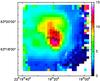 |
Fig. 7 Line width as observed throughout the cloud. The FWHMs were derived from a 2nd moment map of the line emission. Broader profiles appear toward the center (>10 km s-1), where the three infrared sources are located, and narrower toward the ionization front (<5 kms-1). The FWHM that characterizes the gas that surrounds the protostars varies between ~5−10 kms-1. |
Table 1 presents the line parameters as measured toward the IRS 1 and IF positions, applying a single-component Gaussian fit, including both HIFI (Fig. 6) and IRAM (Figs. 4 and 5) observations. The uncertainties quoted for the peak intensities correspond to the observational rms, and the uncertainties for the full width at half maximum (FWHM) and υLSR are from the Gaussian fits to the peak position. The width of the lines varies throughout the cloud, showing broader profiles toward the center of the map, where the three infrared sources are located and narrow toward the ionization front (Fig. 7). Since we are interested in the quiescent gas and thus the narrow component of the lines, we used observed and computed peak intensities in our calculations, because the narrow component dominates the total peak intensity of the lines (≥50%). With this method we limit the effects from outflow activities on our calculations, but we cannot totally exclude them. The outflow contamination of the line is stronger toward the central sources where the integrated contribution of the broad and narrow components is comparable and weaker in positions away from the sources where the narrow component provides 70−85% of the total peak intensity. We restricted the peak intensity analysis to a velocity window of the width of the FWHM of the lines around the 13CO 1−0 line. In this way we always model the same quiescent component.
4. Physical conditions
4.1. RADEX fitting
4.1.1. Method
We used the non-local thermodynamical equilibrium (LTE) radiative transfer program RADEX (van der Tak et al. 2007) to compare the observed line intensity ratios with a grid of models for deriving kinetic temperatures, gas densities, and column densities. As model input we used the molecular data from the LAMDA database (Schöier et al. 2005) and CO collisional rate coefficients from Yang et al. (2010). RADEX predicts line intensities of a molecule for a given set of parameters: kinetic temperature, column density, H2 density, background temperature, and line width.
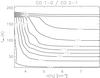 |
Fig. 8 Line ratios of CO 1−0/CO 2−1 as a function of kinetic temperature and H2 density for column density NCO = 1018 cm-2. |
In the density range relevant to S 140, the CO 1−0/2−1 ratio is a good tracer for kinetic temperatures. This is demonstrated in Fig. 8, which shows the CO 1−0/2−1 line ratios for a CO column density of 1018 cm-2. For typical gas temperatures, we see that these ratios are insensitive to H2 density for values >104.5 cm-3, well above the critical density of both transitions. At this point we should also point out that at low kinetic temperatures, this ratio is also not a good indicator of kinetic temperature at the accuracy needed to distinguish between 30 K and 60 K. In this temperature range of CO 1−0/2−1 ~ 1.0 ± 0.1, one would have to know the main beam temperature reliably to within 10% to trust the solution to the kinetic temperature to within ±15 K. Given the uncertainties in antenna and receiver calibrations, beam sizes, sidelobes, etc., this level of accuracy is difficult to achieve. One main source of uncertainty is the coupling efficiency of the beam to the source structure. For sources larger than the main beam, the 30 m errorbeams (and sidelobes) contribute to the coupling. At 230 GHz, the main beam efficiency of the 30 m is high, 60%, and the three 30 m error beams contribute 26% to the total power received by the beam pattern. In addition, assuming a reasonable source size of about 1′, only the main beam and first error beam contribute. Because the first error beam contains only 4% of the total beam power, the correction factor for the antenna temperatures, Feff/Beff decreases only a little, from 92/59 = 1.56 to 92/63 = 1.46. However, it is not the purpose of our paper to deconvolve the channel maps for the error beams or to provide a full accounting of the error budget contributing to Tmb.
4.1.2. Assumptions
For the CO 1−0, CO 2−1, 13CO, and C18O peak intensities (~ 3 × rms), we performed a χ2 minimization to fit the gas kinetic temperatures and column densities assuming that all lines arise from the same gas. For more accurate modeling, the CO 2−1 map was convolved to a lower angular resolution in order to be consistent with the other lines (~21″). The χ2 function was computed as the quadratic sum of the differences between the observed and the synthetic line intensities for a range of kinetic temperatures (10 K <Tkin< 200 K) and column densities (1013 cm-2<NCO< 1019 cm-2), which are values that are consistent with the expected ones for such a region (e.g., van der Tak et al. 2000; Spaans & van Dishoeck 1997; Poelman & Spaans 2006; Hüttemeister et al. 1993).
An additional free parameter in RADEX is the temperature of the background radiation field that may pump the line transitions. We adopted the value of 2.73 K for all our calculations since the cosmic background radiation (CMB) peaks at 1.871 mm, and it is the prominent component at millimeter wavelengths. We used a fixed line width value of 3.5 km s-1 that approximates the value that we have measured throughout the cloud for the narrow component. Finally, to compute the intensities of the isotopic lines, we assume fixed isotopic ratios of 12CO /13CO = 60 and C16O/C18O = 560 (Wannier 1980; Wilson & Rood 1994).
4.1.3. Gas density
Previous studies have shown that the S 140 region contains gas with nH2~ 105 cm-3. Poelman & Spaans (2006) report clumpiness in the region and give a value of nH2 ~ 104 cm-3 for the interclump medium and ~4 × 10⁵ for the clump gas.
Figure 8 shows that it is impossible to derive the gas density from the low-J lines of CO (2−1, 1−0) for densities of nH2 ~ 105 cm-3 or above. A reliable determination of the gas density was thus only possible for those parts of the map where the HIFI cuts provided additional high-J line data. Here, we performed a three-parameter RADEX analysis, fitting the CO 1−0, CO 2−1, CO 9−8, 13CO 1−0, 13CO 10−9 and C18O 1−0 lines convolved to the same resolution (21′′), to determine the nH2. The result is shown in Fig. 9. This fit proves that, at least along the cuts, we find gas densities everywhere, well above nH2 = 105 cm-3, where the CO 1−0/CO 2−1 line ratio can be directly used as a temperature measure. In this way we can be sure to avoid the regimes where the ratio is sensitive to the H2 density.
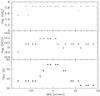 |
Fig. 9 Profiles of gas temperatures (bottom), column densities (middle), and nH2 densities (top) along the HIFI cut, as resulting from the 3−free parameter fitting process to the 30 m and HIFI data. The resulting nH2 densities are always >105 cm-3 throughout the HIFI cut. |
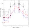 |
Fig. 10 Temperatures of dust (red line) and gas along the HIFI cut. The gas temperature as derived fitting low-J lines (IRAM data, blue line) is systematically lower than the derived gas temperature fitting both low and high-J lines (IRAM and HIFI data, black line). Tgas (from both low and high-J lines) is systematically higher than Tdust, at least along this cut. The errors vary between ~5−15% throughout the cut with the higher accuracy close to the central position. |
To assess the reliability of the results, we performed two separate RADEX fits along the cuts where the 9−8 and 10−9 transitions of CO and the isotopologues were observed by HIFI. In the first fitting approach, we fixed nH2 to 105 cm-3 and fit only the low-J CO lines observed by IRAM and all the lines (Fig. 10). The second fit uses all the lines and treats the gas density as a free parameter in the range between 7 × 103 cm-3 and 7 × 105 cm-3 as in Fig. 9. The best fit of the latter occurred for nH2> 105 cm-3. Adding the higher-J lines drives the fit to systematically higher kinetic temperatures by about ~5−15 K (Fig. 10). The opacities of the lines are found to be in the following ranges: CO 1−0: 16−45, CO 2−1: 52−154, CO 9−8: 3.6−65, 13CO 1−0: 0.3−0.8, 13CO 10−9: 0.017−0.38, and C18O 1−0: 0.025−0.09. As an attempt to test how much the optically thin 13CO 10−9 line influences the solution, we reran our calculations, applying a double weight for this line. The resulting kinetic temperatures changed by  K, that is, inside the range of the reported errors.
We ran the same kind of analysis toward the two positions with most lines observed4 (see Table 1). Toward IRS 1, the full analysis provides a gas kinetic temperature of  K and a column density of
  cm-2, while the same procedure using only the IRAM data results in a kinetic temperature of
  K and a column density of
  cm-2. Toward the IF position, the full dataset indicates a kinetic temperature of
  K and column density of
  cm-2, while the IRAM data only result in a kinetic temperature of
  K and column density of
  cm-2. The gas temperatures obtained when using only the low-J lines from IRAM underestimate Tgas, providing a lower limit of gas temperatures (Yıldız et al. 2013). The major and minor axes of the resulting χ2 contours were used as the error bars of the two parameters.
For a more accurate determination of the H2 density, tracers such as CS 2−1/3−2 and HCO+ 1−0/3−2, are more reliable (van der Tak et al. 2007), but were not observed. Snell et al. (1984) derived a density of 5 × 105 cm-3 toward IRS 1−3 using four CS transitions that agree with the value we derived. In addition Goldsmith & Langer (1999) performed a LTE population diagram analysis toward IRS 1 using the same CS dataset and derived a kinetic temperature between 30−50 K, which is lower than our value probably due to the effect of their larger beam size.
4.1.4. Kinetic temperature and column density distribution
The resulting maps of kinetic temperatures and CO column densities are shown in Fig. 11. We find a kinetic temperature of ~ 55 K toward the center and ~ 45 K toward the ionization front, while the rest of the cloud is characterized by lower temperatures (25−40 K; Fig. 11). The column density toward the center was found to be the highest, with a value of ~ 6.5 × 1018 cm-2, while toward the IF was found to be ~ 1.1 × 1018 cm-2. The lowest column density that was determined throughout the cloud is ~ 1.4 × 1016 cm-2. The gas temperature map obviously reflects the different heating contributions by the embedded cluster of the three high–mass YSOs (IRS 1 to 3) in the center and from the external B0V star HD 211880 toward the IF.
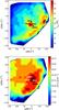 |
Fig. 11 Kinetic temperature (top) and column density (bottom) maps of S 140 (all lines > 3 rms). They are both higher toward the embedded infrared sources and lower throughout the rest of the cloud. The kinetic temperature rises again toward IF, but remains below the value toward the center. |
4.2. Dust analysis
Prior to any radiative transfer modeling of the dust in this region (Sect. 5), we here estimate the rough temperatures and optical depths relevant to the dust distribution. For this we used the PACS/Spec continuum data from 73−187 μm, which covers the peak of the SED over the entire region mapped with PACS well (Fig. 12). To analyze our dust continuum observations, we used two subsets of the PACS and SOFIA images. To compute a luminosity map, we used the 11−187 μm images all as reconvolved to the 187 μm resolution (13′′). At each 1′′ pixel of the computed image we integrated the flux density from 11.1−187 μm and included a linear extrapolation to zero flux level beyond 187 μm, which typically results in only a few percentage points added to the total. We believe the absolute uncertainties in this map are approximately 15% based on the absolute calibration uncertainties of all the input data. The relative uncertainties are probably much less, ±5%, since there is very little luminosity shortward of 10 μm and longward of 200 μm.
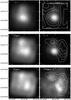 |
Fig. 12 Left column: PACS/Spec continuum images (5 × 5 spatial array of 9′′ pixels regridded to a 1′′ grid) with contours of 37 μm (SOFIA) emission overlaid showing the positions of IRS 1, 2, and 3. Right column: top – total luminosity image with contours of fitted dust temperature at 70, 65, 60, ...K; center – luminosity image with contours of fitted dust optical depth at levels of 0.1, 0.15, 0.2, and 0.25; bottom – 450 μm SCUBA image with the same fitted dust optical depth contours overlaid. |
We computed color-temperature and optical-depth values at each spatial point on the 1′′ grid by fitting a blackbody function modified by a λ-1 dust emissivity variation. The peak dust optical depths at the shortest wavelength are likely to be several × 0.1, but still less than unity, so we did not include any effects from optical thickness in these estimates. A comparison of the luminosity, color temperature, and optical depth maps and several images is shown in Fig. 12. These images show a number of important qualitative properties of the dust emission. First, there is a clear and relatively smooth change in source morphology from that at 73 μm, which is similar to the 10−37 μm images, to the morphology at 187 μm, which is beginning to show many of the features of the SCUBA 450 μm map. Second, the dust optical depth we derived from the Herschel data is very similar to the 450 μm emission map. Finally, the luminosity image shows clearly that IRS 1 is the main luminosity source in the region, followed in importance by IRS 2 and then IRS 3. There is no obvious luminosity peak within the area of strongest 450 μm emission, so this is probably a peak in the column densities of dust and gas.
One uncertainty of the dust temperature may stem from the assumed spectral properties of the dust grains, in particular the assumed spectral index β. Recent observations of dust in the diffuse ISM with the Planck mission indicate a mean dust temperature of ~20 K and dust emissivity index of ~1.6 (Jones 2014). This is clearly higher than the value of β = 1 assumed here, which is more appropriate for dense clouds (Ossenkopf & Henning 1994). Since our region is denser than the majority of those observed with Planck, we can consider the value of β = 1.6 as an extreme upper limit for our case. When we fit a blackbody function modified by a λ-1.6 to derive the dust temperatures, we obtain temperatures that are lower by 5−20 K than the values from the adopted λ-1. We conclude that in our analysis we derive an upper limit of dust temperatures.
4.3. Comparison of dust and gas temperatures.
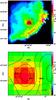 |
Fig. 13 Gas kinetic temperature map toward the IRAM field (low-J analysis) with overplotted contours of dust temperatures (top) and zoomed in PACS field (bottom). The levels of contours are 55 K (inner) until 35 K (outer) using steps of 5 K. The color bar indicates the values of kinetic temperature. The 2 temperatures from this analysis seem to agree well, but the gas kinetic temperatures are underestimated for ~7−12 K (Fig. 10). |
For a direct comparison with the gas kinetic temperature map, the dust temperature map was convolved to the same angular resolution (~21″). The comparison between gas and dust temperatures from the low-J line analysis (Figs. 10 and 13), shows a very similar spatial structure around the infrared sources. The higher-J lines from HIFI, though, reveal that the low-J analysis underestimates the gas temperatures (see Sect. 4.1.3). Assuming that this trend applies to the entire region and not only along the cuts (Fig. 10), we conclude that the gas temperature is higher than the dust in the entire region.
The temperature difference of ~5−15 K revealed from the complete analysis lies outside the uncertainty range of the 2−7 K and indicates a more efficient gas heating even at densities ≥104.5 cm-3 where the two components are relatively well coupled.
To illustrate the expected overall temperature dependence, we show in Fig. 14 the outcome of a simplified PDR model for S 140 computed with the KOSMA-τ PDR code (Röllig et al. 2006, 2013). It shows the temperature profile for a spherical PDR clump with a mass of 100 M⊙, mimicking a plane–parallel PDR, and a surface density of 105 cm-3 illuminated by an UV radiation field of 100 Draine fields (Draine 1978). For reference, the figure shows the visual extinction AV as a function of the depth into the cloud. The model shows that through almost all of the whole cloud, the gas temperature is higher than the dust temperature by about 15 K for AV = 0.1 but by only 2 K deep in the cloud. The small kink in the gas temperature around AV = 1 stems from H2 formation heating on PAHs and the temperature structure of the PAHs. Overall, the model confirms that for a homogeneous medium, we expect the same temperatures for gas and dust within our observational measurement errors for visual extinctions into the cloud of more than about 0.5, i.e. for depths of one arcsecond and more at the distance of S 140. The extended hot gas therefore cannot be explained by a homogeneous extinction of the UV radiation but requires some clumpy structure, allowing for deeper UV penetration.
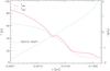 |
Fig. 14 Dust and gas temperatures in a spherical PDR clump with a surface density of 105 cm-3 illuminated by an UV radiation field of 102 Draine fields. Gas temperatures generally exceed the dust temperatures (see Röllig et al. 2013, for a more general discussion). The green dash-dotted line shows the visual extinction AV as a function of the depth into the cloud. |
5. Effect of density gradients
Assuming uniformly distributed densities and temperatures for each spatial position was a good approach for the extended gas and dust in S 140, but detailed modeling is required for the more complicated dust and gas structures that are expected to be close to the infrared sources. The radiation we receive is a result of various processes, including the interaction with the surrounding dust. For a more precise physical approach, the radiative transfer calculations should include the original radiation, characteristics of the dust grains and the dust density distribution. Density gradients have been revealed for S 140 in previous studies that include Harvey et al. (1978), Gürtler et al. (1991), van der Tak et al. (2000), and Maud & Hoare (2013). We first performed an advanced dust modeling taking dust density gradients into account. Then we applied the best-fit derived dust mode to predict the CO intensities using an advanced radiative transfer code (i.e., RATRAN; Hogerheijde & van der Tak 2000), as an attempt to test the accuracy of our dust model comparing with the gas observations and predictions.
5.1. Dust modeling: an approach
It is clear from all the infrared and sub-mm images of the S 140 cluster that there are several luminosity sources in the central arcminute and that the dust distribution is unlikely to be spherically symmetric. This implies that any simple model of the dust heating will be limited in its applicability. We have, however, identified some goals to address with simple radiative transfer models. First, since all the observational data suggest that IRS 1 is the dominant luminosity source, we believe that we can determine some rough properties of the dust distribution close to it by ignoring the heating from IRS 2 and 3 and any of the other much lower luminosity objects that are part of the embedded stellar cluster around IRS 1. To this end, we concentrate on two observables for the model comparison for IRS 1: (1) the SED of IRS 1; and (2) the spatial flux distribution from the center to the south of IRS 1 where there are no strong obvious nearby heating sources seen in the infrared that are likely to contribute significantly to the dust heating. A second goal is to try to understand whether the peaks in the 450 μm image can be due to some unusual dust distribution to the west and southwest of IRS 1 with no additional internal heat source or if some internal heating is required to explain them. For example, the recent observations and modeling by Maud & Hoare (2013) suggest an internal source within the strongest 450 μm peak to the southwest of IRS 1, i.e. SMM 1 (ΔRA: –14.22′′, ΔDec: –7.90′′, relative to IRS 1).
The approach we took to addressing these goals involved several steps that we discuss in detail in the following sections. First, we tried to find what properties of models were required to provide a fit to the observed SED from the central pixel centered on IRS 1 and to the source profile of IRS 1 to the south, assuming a single, spherically symmetric dust distribution. This model was then used as a starting point for subsequent stages. The second step was to create a model made from hemispheres of two different spherically symmetric dust distributions. Though this model is simplified, it seems likely that far from the boundary region, such a combination can give insight into the degree to which such a dust distribution might reproduce the observed source structure to the west and southwest of IRS 1 by assuming a higher column density in this region than to the south and east of IRS 1. For this comparison we used the source profile extending southwest along a line from IRS 1 to and beyond the position of SMM 1, as given by Maud & Hoare (2013). As an alternative to the two-hemisphere model, we also attempted to fit the profiles along this line with two separate sources by using the superposition of two spherically symmetric models with different central source luminosities and very different dust distributions separated on the sky by ~16′′ to attempt to reproduce the observed 1D flux profile between IRS 1 and the position of SMM 1 southwest of it.
In testing these last two model variations, the two-hemisphere construction and the two-source construction, it became clear that the best results would probably result from a combination of both features. Such a model would also be most realistic in light of the much higher dust column density to the west and southwest as indicated both by the SCUBA maps and our Herschel maps, together with the presence of the compact sub-mm/mm source found by Maud & Hoare (2013). After constructing a few such models, we realized that with so many free parameters, it would be difficult to find the range of well-fitting parameters without testing the fits over a large, multi-dimensional grid. This process represented the final stage of modeling for IRS 1, and we now describe the process and results. Figure 15 shows a schematic diagram of the model for IRS 1 and the sub-mm peak to the southwest.
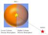 |
Fig. 15 Schematic diagram in the place of the sky of the model for IRS 1 and the sub-mm peak (ΔRA: –14.22′′, ΔDec: –7.90′′) to the southwest. The distance between the 2 positions is ~0.06 pc. |
For all the models we used the DUSTY code (Ivezic et al. 1997) and converted the dimensionless output values to those appropriate for the assumed distance of S 140, 746 pc (Hirota et al. 2008) and the assumed luminosity (discussed below) for comparison with the observations. We tried models with two different dust compositions: the first was a mixture of 90% DL silicates (Draine & Lee 1984) and 10% amorphous carbon, both of whose optical constants are distributed with DUSTY. The second was OH5 (Ossenkopf & Henning 1994) dust, for which a number of authors (e.g., van der Tak et al. 1999) have suggested that they may be more appropriate in dense star-forming regions where significant grain growth may have taken place. We found similar quality fits with comparable dust density distributions for both grain compositions. The 1 μm optical depths were, however, about twice as high with the DL/carbon dust than with the OH5 grain properties owing to the overall difference in the slope of the dust optical depth between 1 and 100 μm. The output of the “observed” profile of each model at each wavelength was first interpolated onto a 3050 × 850 grid with spacing equivalent to 0.05′′. We then convolved this image with the appropriate observing beam to compare with the observed images (not those convolved to the 187 μm resolution). Finally, we “observed” this image with a 9′′ square beam that we moved across the image in 1′′ steps to compare with the observed images whose fluxes we also added into such a moving 9′′ square beam. For the shorter wavelength images, we also applied the same 9′′ square pixel flux summation for comparison between the models and observations.
5.2. Model grid
The model that we used is described by nine parameters, four for the eastern half of IRS 1, four for the western half, and one, luminosity, for SMM 1. Table 2 lists these nine parameters, as well as the range of values tested in a grid, thereby allowing all possible combinations of these values (150 000 models). A preliminary run of ~800 000 models showed that the results were quite insensitive to the value of parameter 4, the radius where the slope of the density gradient changed in the high-column hemisphere, so it was fixed at a value of 300× the inner radius. Similarly, the value of the density gradient in this inner region affected the final results only slightly, so this was fixed at a value 0.4 (ρ ∝ r-0.4). Therefore, for the final results there are seven free parameters.
Model parameters and range for grid fitting with OH5 dust.
To select the most likely models and to estimate the range of values that produces a reasonable fit, we characterized the model fits by the χ2 that we computed as follows. We parameterized the observations and accompanying model fits into 30 values of the SED and the source profile at various wavelengths. Since the signal-to-noise ratio of almost all the observations is quite high, the systematic uncertainties of the observations (e.g., pointing) dominate the true uncertainties. We, therefore, assigned somewhat arbitrary values to the assumed errors for these 30 values to drive the fitting to something “reasonably” close to the observations. Table 3 lists these properties of the observed data and uncertainties.
Parameters and assigned relative uncertainties used to compute χ2 of fit to IRS 1.
As shown in the table, the parameters used to calculate the χ2 of the fit included the SED between 37 and 450 μm, the flux at the position of SMM 1, the relative flux at 37−450 μm at offsets of 9′′ and 18′′ to either side of the position of IRS 1 (i.e., one pixel and two pixels), and finally, the observed luminosity at those four offset positions (not relative to the central pixel). We intentionally did not include the portion of the SED shortward of 37 μm, since the dust close to the central source of IRS 1 is likely to be distributed in a disk-like configuration, which would lead to more flux escaping at shorter wavelengths than is consistent with the assumption of spherical symmetry. Likewise, we did not attempt to fit the total observed luminosity at the central pixel since much of the luminosity is emitted shortward of 37 μm. To estimate the range of model parameters that provided a “good” fit to the data, we assigned probabilities to each model equal to exp( − χ2/ 2).
The best-defined parameter values from the probability plots are the mild density gradient away from IRS 1 of ρ ∝ r-0.4 and the outer radius of 1500 times the inner radius. The optical depth is relatively well defined by Av ~ 40, though there is a better-defined joint probability that includes the optical depth and density gradient. The peak probability for the luminosity of SMM 1 is 100 L⊙, but there is a wide range of values with reasonable probability from ~50 L⊙ to 300 L⊙. The parameters of the dense material to the southwest of IRS 1 are not well defined for the most part. Interestingly, the gradient of the material in the outer area (300−1500 × the inner radius) seems to have a very probable range similar to the range found for the rest of the cloud around IRS 1; i.e., r− p with p ~ 0 − 0.5. There is a significant joint probability distribution between the outer gradient to the southwest and the luminosity of SMM 1. This is to be expected, since the effects of a steeper gradient can be largely compensated for by increasing the luminosity of SMM 1. Although the most probable models have Av = 40, the probability distribution suggests that the most probable range is 40−60, i.e., somewhat higher than the gradient to the south.
Examples of the model-fit profiles from one of the two lowest χ2 (2.7) fits, as well as the SED, are shown in Figs. 16−18. The model profiles shown in Fig. 16 display a less than perfect fit at the longest wavelengths in our PACS observations, 140−190 μm. This effect has been driven by two parts of the fitting process: that we did not include the relative flux at the central (IRS 1) position in the χ2, and that it proved quite difficult to find any models that dropped as slowly as the observations at the ends of the profiles 18′′ away from the center. The properties of the models that do the best job fitting the profiles 18′′ away from IRS 1 also drive the relative 187 μm profile to be too high at IRS 1 compared to its value at SMM 1. In some simple tests, we have found that if we added an artificial floor to the model fluxes beyond 125 μm, we could fit the longer wavelength profiles significantly better.
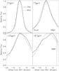 |
Fig. 16 Observed and model profiles at four PACS/Spec wavelengths normalized to the peak along a line from the south into the center of IRS 1 and then out along a line to the southwest extending to the SMM 1 source. |
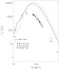 |
Fig. 17 SED for a typical model fit with low χ2. The solid line shows the total flux coming from the warm hemisphere, and the dotted line shows the SED for the fraction of the flux coming from the cold hemisphere. The plotted symbols show the observed and model fluxes for the fraction within the central 9′′ PACS pixel. |
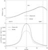 |
Fig. 18 Profiles along the same line as used in Fig. 15 for the 450 μm flux (top panel) and the total luminosity (bottom panel). We note the significant mismatch in the central region, which is due to not trying to fit the 5−30 μm luminosity, since some of it likely arises from an axisymmetric disk rather than the spherical model used here. |
5.3. IRS 2 and 3
The most important factor affecting our attempts to model IRS 2 and 3 is that the flux from our well-fitting models for IRS 1 is a significant fraction of the total flux at the positions of IRS 2 and 3. This means that any models we make for IRS 2 and 3 will have an additional large uncertainty due to the uncertainty in the true contribution from IRS 1. For example, the model flux from IRS 1 at the position of IRS 3 is more than 50% of the total at wavelengths beyond 120 μm. We have therefore computed models for roughly a dozen possible configurations for each source to develop some feeling for the range of likely parameters, but the uncertainties in our estimates are quite large.
For IRS 3 we used a profile that begins on the east side of the source and, after passing through the center, goes straight to the south in order to minimize the confusion from IRS 1. An additional complication is that IRS 2 is clearly elongated in the east-west direction in the mid-IR, and there is a clear position shift in the same direction between the mid-IR and our PACS data. This suggests that there are at least two relatively luminous objects heating the dust at the position of IRS 2 with different dust optical depths, higher to the east and lower to the west. The position shift between 12 and 73 μm is only a few arcsec, which is a fraction of our PACS native pixel size. Therefore, for IRS 2 we used a source profile from east to west and a model like the one in the “two-hemisphere” modeling for IRS 1, with a hot, lower-optical-depth dust distribution on the western side and a cold, higher-optical-depth distribution offset 4′′ to the east. Such a model will not accurately reproduce the source elongation, but should roughly fit the overall SED and some part of the profiles. Figures 19−22 show the model SED and profile fits for some representative models that illustrate both the features that can be fit reasonably well as for those that are difficult to fit.
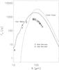 |
Fig. 19 Model and observed SED’s for IRS 2. The solid line shows the model fluxes for the hotter source to the west in the model, while the dashed line shows the fluxes for the colder source to the east. The symbols show the model and observed fluxes in the central 9′′ pixel as in Fig. 16. |
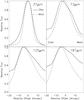 |
Fig. 20 Model and observed profiles for IRS 2 as in Fig. 15, but along a straight east–west line. |
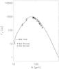 |
Fig. 21 Model and observed SEDs for IRS 3. |
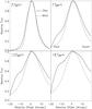 |
Fig. 22 Model and observed profiles for IRS 3 along a line extending into the source center from the east and then outward to the south. |
For both of these sources, we did attempt to fit the mid-infrared fluxes in the SED, unlike for IRS 1. The very extended tail of emission on the west side of IRS 2 at 125 and 187 μm coincides well with the increase in optical depth seen in our data and the SCUBA maps in that area. We have not tried to fit this with these simple models. The bump seen on the eastern side of the long wavelength profiles for IRS 3 is coincident with the outermost pixel of our mapping, so we did not try to fit it.
The most well-defined results seem to be that 1) the dust distribution around both sources is likely to be quite flat; and 2) the luminosities of the sources are likely in the range of 1000−2000 L⊙, as shown in Table 4. The first could be consistent with very little dust around them that is associated with them, but mostly with the extended distribution around IRS 1.
Model parameters for symmetric fit with OH5 dust to IRS 3 and “two-hemisphere” fit to IRS 2.
5.4. Gas modeling
To test our best-fit DUSTY model, we ran the Monte Carlo radiative transfer code RATRAN (Hogerheijde & van der Tak 2000), which treats the physical structure of the sources, including temperature and density gradients. RATRAN estimates the local radiation field at all line frequencies taking the radiation field from every other position in the cloud into account. We ran RATRAN applying the best-fit DUSTY model and assuming the same temperature for dust and gas toward IRS 1 in order to model the CO 1−0, CO 2−1, CO 9−8, and isotopologue lines and to compare them to the outflow–subtracted component from the observations (Fig. 23). The outflow emission was subtracted since the DUSTY models focus on the bulk of the quiescent dense gas where the outflow cavities are negligible. For the outflow subtraction, we applied a two-component Gaussian fit to the observed lines toward IRS 1 followed by subtraction of the broad component.
For our calculations we defined a grid of 18 spherical shells for the eastern (lower density) hemisphere (constant ρ ∝ r-0.4) and 22 for the western (high density) hemisphere by applying the density gradients as obtained from the DUSTY model. The inner and outer radii were taken from the DUSTY model and were set to 2.08 × 1014 cm and 3.12 × 1017 cm, respectively, while the inner H2 density was set to 9 × 105 cm-3. This value was derived from the best-fit dust model assuming that the gas is entirely molecular and using a mean gas mass per hydrogen of 1.4 amu and a gas-to-dust ratio of 100.
Dust continuum radiation is considered using the same OH5 opacities as in the DUSTY model. We assume a static envelope without infall or expansion, a fixed CO abundance of 10-4, and a turbulent line width of 3.5 km s-1.
Figure 23 shows the lines of CO 1−0, CO 2−1, and CO 9−8 and isotopologues as observed toward IRS 1 overplotted with the convolved (~21′′) synthetic emission as calculated with RATRAN. We show the resulting line profiles for both the low-density east hemisphere and the high-density west hemisphere from the DUSTY models. With the exception of the low-J transitions of the isotopologues, we observe no significant differences between the two cases. The fit between observed and modeled lines shows that the low-J lines are reproduced but the higher-J lines are significantly underestimated, especially for the isotopologues. The model cannot reproduce the highly excited lines tracing high column densities of warm and very dense gas. An adapted kinematic structure and/or clumpiness can potentially remove the modeled self-absorption dip of the optically thick 12CO lines, but treating these effects is beyond the scope of this work. Models with Tgas>Tdust, as inferred from the simple analysis in Sect. 4.3, would probably be able to reproduce the high-J lines without significantly affecting the low-J lines. Local density enhancements can be an alternative solution, if the total mass of the cloud is conserved, such as in a clumpy or disk/outflow geometry.
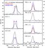 |
Fig. 23 Outflow-subtracted spectra of CO 1−0, CO 2−1, CO 9−8, 13CO 1−0, 13CO 10−9, C18O 1−0, and C18O 9−8 (black) as observed toward IRS 1, overplotted with the synthetic emission as calculated with RATRAN, after having applied the lower density east hemisphere from DUSTY models (red) and the high density west hemisphere (blue). We observe no significant differences between the two cases with the exception of the low-J transitions of the isotopologues. While the model fits the observations for the lower transition lines well, it fails to reproduce the observed higher transition lines. |
6. Discussion and conclusions
Based on PACS, HIFI, and IRAM data, we find a wide range of dust and gas temperatures in the S 140 region. The warmest gas (~ 55 K) is around the three infrared sources, while the surrounding environment is characterized by colder temperatures (~25−35 K). The gas temperature increases toward the southwestern edge of the cloud (IF), reaching values of ~40−45 K. This rise in temperature is the result of the UV heating from the external B0V star HD 211880 that lies ~7′ southwest of the edge of the cloud. Unfortunately, we cannot compare the gas and the dust temperatures toward IF because of the smaller area that our continuum dust observations cover.
We find that the dust density gradient around IRS 1 is likely to be shallower than the best fits found in some earlier models in order to explain the spatial structure we find in the far-IR. The strong emission to the west and southwest of IRS 1 at wavelengths longward of 100 μm can possibly be explained by heating from IRS 1, along with a strongly increasing density to the west and southwest. We do, however, find a significantly better fit by interpreting the emission as arising from two or more separate sources with very different amounts of dust around the sub-mm source compared to IRS 1. The luminosity of the internal source at the sub-mm peak is likely to be a few ×102L⊙ in this model. This model with an internal luminosity source at the sub-mm peak is consistent with the study of Maud & Hoare (2013), who find that the two strongest 1.3 and 2.7 mm emission peaks are the position of IRS 1 and SMM 1. Because our models did not include outflow cavities or clumpiness, it is possible that this conclusion should be revisited after more extensive modeling.
The gas temperature analysis, including both high and low-J lines, was possible only along the HIFI cut and revealed a systematic excess of gas temperatures against dust temperatures. This result indicates a more efficient gas heating even at densities ≥104.5 cm-3 where the gas and dust are usually expected to be in thermal equilibrium. New SOFIA/GREAT mapping observations of CO 13−12 and 16−15 confirm this excess of the gas temperature, and the results show an even greater gap in energy between the gas and dust components (Ossenkopf et al. 2015). The high-J lines show that a limitation to the low-J analysis (IRAM) causes an underestimate of the gas temperatures by ~7−12 K and thus provides only a lower limit of the temperatures in the cloud. Thus it is most likely that the gas temperature is higher than the dust also in the whole field. Unfortunately, the higher-J lines do not cover the entire region so that we cannot prove this. The detailed gas modeling also indicates that DUSTY results are good estimates of the temperature and density structure around IRS 1 for the colder gas, but there is an excess of warm dense gas that cannot be reproduced by these models (i.e., CO 9−8). The attempt to fit those higher transition lines by modeling hotter gas than dust and/or applying different geometries (i.e., clumps, disk geometry) that would increase the density locally but not the total amount of mass is in our future plans.
The observed gas temperature excess cannot be explained by a higher cosmic ray ionization. Van der Tak & van Dishoeck (2000) reported a cosmic ray ionization rate of <10-16 s-1, which is too low to provide a major gas heating in S 140. Some gas heating may be due to outflow activities. In the RADEX and RATRAN analysis, we focused on quiescent gas and limited the contribution from protostellar outflows. However, it is possible to have high-velocity motions perpendicular to the line of sight. In addition, the larger difference between gas and dust appears in points close to the observed outflow by Preibisch & Smith (2002). A collection of shocks, longitudinal and transversal to the walls of the possible inner cavity around the IR sources, will contribute to the emission at the ambient velocity. Oblique shock components are thus a plausible scenario for a somewhat more efficient heating of the gas than of the dust.
The most probable scenario appears to be the deep UV radiation in a clumpy medium. Dust is heated by UV and IR, while gas is heated by processes driven only by UV with the main one being the photo-electric heating (Hollenbach & Tielens 1997; Röllig et al. 2013). In the vicinity of any stellar or protostellar source, the gas is much hotter than the dust when dust and gas are not coupled. Dust-gas collisions try to equilibrate them if the density is high enough. The dust quickly attenuates the UV so that the gas becomes colder when going away from IRS 1. The penetration of the IR is deeper (lower extinction in IR compared to UV), so that the decay in the temperature of the dust is shallower than for the gas. However, since we observe that the gas remains hotter than the dust over a relatively large distance from IRS 1, the UV seems to penetrate much more deeply into the cloud than expected from a homogeneous medium. The natural explanation is a clumpy medium where there are always enough rays between the clumps that still allow UV propagation to keep the gas warm.
Previous studies already report that S 140 is clumpy (e.g., Kramer et al. 1998). Battersby et al. (2014) performed a similar study to determine the relationship between gas and dust in a massive star-forming region (G 32.02+0.05) by comparing the physical properties derived from each, using NH3 transitions. In that study similar temperature differences are reported with the dust temperatures being lower than gas temperatures (by a few K) in the quiescent region, indicating that gas and dust might be not well-coupled in such environments. Differences between gas and dust temperatures in several environments with high densities have been reported in more studies (Papadopoulos et al. 2011; Hollenbach & Tielens 1999).
Our observations trace warm and cold dust but also warm and less warm gas, because we have multiple transitions of CO. The low-J lines tend to show the surface of clumps since they are optically thick but the optically thin isotopologues 13CO 1−0 and C18O 1−0 carry information from deeper positions. Furthermore, the higher transitions CO 9−8 and 13CO 10−9 trace warmer gas, but they also arise from deeper positions. That we have optically thin lines and the dust emission is optically thin confirms that we trace the whole line of sight both in gas and dust and thus the observational limitations can probably be excluded.
The values were calculated using Einstein coefficients and collisional rates (Eq. (2)) from Yang et al. (2010).
m96bu47199708210025 from http://www.cadc-ccda.hia-iha.nrc-cnrc.gc.ca/en/jcmt/
GILDAS is a radio-astronomy software developed by IRAM. See http://www.iram.fr/IRAMFR/GILDAS/
For the low-J CO data we extracted the points from the IRAM maps closest to HIFI pointing observations with no more than 3″ offset.
Acknowledgments
The authors would like to thank the referee for a careful reading of the manuscript and for providing helpful comments and suggestions that improved the paper. P.H. was supported through the NASA Herschel Science Center data analysis funding program, by a NASA contract issued by the Jet Propulsion Laboratory, California Institute of Technology to the University of Texas. V.O. was supported through the Collaborative Research Center 956, subproject C1, funded by the Deutsche Forschungsgemeinschaft (DFG). A.F. thanks the Spanish MINECO for funding support from grants CSD2009−00038 and AYA2012−32032. HIFI has been designed and built by a consortium of institutes and university departments from across Europe, Canada, and the United States under the leadership of SRON Netherlands Institute for Space Research, Groningen, The Netherlands, and with major contributions from Germany, France, and the US. Consortium members are: Canada: CSA, U.Waterloo; France: CESR, LAB, LERMA, IRAM; Germany: KOSMA, MPIfR, MPS; Ireland, NUI Maynooth; Italy: ASI, IFSI–INAF, Osservatorio Astrofisico di Arcetri-INAF; Netherlands: SRON, TUD; Poland: CAMK, CBK; Spain: Observatorio Astronómico Nacional (IGN), Centro de Astrobiologa (CSIC-INTA). Sweden: Chalmers University of Technology – MC2, RSS and GARD; Onsala Space Observatory; Swedish National Space Board, Stockholm University – Stockholm Observatory; Switzerland: ETH Zurich, FHNW; USA: Caltech, JPL, NHSC.
References
- Aniano, G., Draine, B. T., Gordon, K. D., & Sandstrom, K. 2011, PASP, 123, 1218 [NASA ADS] [CrossRef] [Google Scholar]
- Battersby, C., Bally, J., Dunham, M., et al. 2014, ApJ, 786, 116 [NASA ADS] [CrossRef] [Google Scholar]
- Crampton, D., & Fisher, W. A. 1974, Publications of the Dominion Astrophysical Observatory Victoria, 14, 283 [NASA ADS] [Google Scholar]
- de Wit, W. J., Hoare, M. G., Fujiyoshi, T., et al. 2009, A&A, 494, 157 [NASA ADS] [CrossRef] [EDP Sciences] [Google Scholar]
- Dedes, C., Röllig, M., Mookerjea, B., et al. 2010, A&A, 521, L24 [NASA ADS] [CrossRef] [EDP Sciences] [Google Scholar]
- Draine, B. T. 1978, ApJS, 36, 595 [NASA ADS] [CrossRef] [Google Scholar]
- Draine, B. T. 2011, Physics of the Interstellar and Intergalactic Medium (Princeton University Press) [Google Scholar]
- Draine, B. T., & Lee, H. M. 1984, ApJ, 285, 89 [Google Scholar]
- Evans, II, N. J., Mundy, L. G., Kutner, M. L., & Depoy, D. L. 1989, ApJ, 346, 212 [NASA ADS] [CrossRef] [Google Scholar]
- Goldsmith, P. F. 2001, ApJ, 557, 736 [NASA ADS] [CrossRef] [MathSciNet] [Google Scholar]
- Goldsmith, P. F., & Langer, W. D. 1978, ApJ, 222, 881 [NASA ADS] [CrossRef] [Google Scholar]
- Goldsmith, P. F., & Langer, W. D. 1999, ApJ, 517, 209 [NASA ADS] [CrossRef] [Google Scholar]
- Gürtler, J., Henning, T., Kruegel, E., & Chini, R. 1991, A&A, 252, 801 [NASA ADS] [Google Scholar]
- Harvey, P. M., Campbell, M. F., & Hoffmann, W. F. 1978, ApJ, 219, 891 [NASA ADS] [CrossRef] [Google Scholar]
- Harvey, P. M., Adams, J. D., Herter, T. L., et al. 2012, ApJ, 749, L20 [NASA ADS] [CrossRef] [Google Scholar]
- Hirota, T., Ando, K., Bushimata, T., et al. 2008, PASJ, 60, 961 [NASA ADS] [Google Scholar]
- Hogerheijde, M. R., & van der Tak, F. F. S. 2000, A&A, 362, 697 [NASA ADS] [Google Scholar]
- Hollenbach, D. J., & Tielens, A. G. G. M. 1997, ARA&A, 35, 179 [NASA ADS] [CrossRef] [Google Scholar]
- Hollenbach, D. J., & Tielens, A. G. G. M. 1999, Rev. Mod. Phys., 71, 173 [Google Scholar]
- Hüttemeister, S., Wilson, T. L., Bania, T. M., & Martin-Pintado, J. 1993, A&A, 280, 255 [NASA ADS] [Google Scholar]
- Ikeda, N., & Kitamura, Y. 2011, ApJ, 732, 101 [NASA ADS] [CrossRef] [Google Scholar]
- Ivezic, Z., Groenewegen, M. A. T., Men’shchikov, A., & Szczerba, R. 1997, MNRAS, 291, 121 [NASA ADS] [CrossRef] [Google Scholar]
- Jones, A. 2014, ArXiv e-prints [arXiv:1411.6666] [Google Scholar]
- Kaufman, M. J., Wolfire, M. G., Hollenbach, D. J., & Luhman, M. L. 1999, ApJ, 527, 795 [NASA ADS] [CrossRef] [Google Scholar]
- Kramer, C., Stutzki, J., Rohrig, R., & Corneliussen, U. 1998, A&A, 329, 249 [NASA ADS] [Google Scholar]
- Maud, L. T., & Hoare, M. G. 2013, ApJ, 779, L24 [NASA ADS] [CrossRef] [Google Scholar]
- Maud, L. T., Hoare, M. G., Gibb, A. G., Shepherd, D., & Indebetouw, R. 2013, MNRAS, 428, 609 [NASA ADS] [CrossRef] [Google Scholar]
- Meijerink, R., & Spaans, M. 2005, A&A, 436, 397 [NASA ADS] [CrossRef] [EDP Sciences] [Google Scholar]
- Minchin, N. R., White, G. J., & Padman, R. 1993, A&A, 277, 595 [NASA ADS] [Google Scholar]
- Mueller, K. E., Shirley, Y. L., Evans, II, N. J., & Jacobson, H. R. 2002, ApJS, 143, 469 [NASA ADS] [CrossRef] [Google Scholar]
- Ossenkopf, V., & Henning, T. 1994, A&A, 291, 943 [NASA ADS] [Google Scholar]
- Ossenkopf, V., Koumpia, E., Okada, Y., et al. 2015, A&A, in press DOI: 10.1051/0004-6361/201526231 [Google Scholar]
- Papadopoulos, P. P., Thi, W.-F., Miniati, F., & Viti, S. 2011, MNRAS, 414, 1705 [NASA ADS] [CrossRef] [Google Scholar]
- Poelman, D. R., & Spaans, M. 2006, A&A, 453, 615 [NASA ADS] [CrossRef] [EDP Sciences] [Google Scholar]
- Poglitsch, A., Waelkens, C., Geis, N., et al. 2010, A&A, 518, L2 [NASA ADS] [CrossRef] [EDP Sciences] [Google Scholar]
- Preibisch, T., & Smith, M. D. 2002, A&A, 383, 540 [NASA ADS] [CrossRef] [EDP Sciences] [Google Scholar]
- Roelfsema, P. R., Helmich, F. P., Teyssier, D., et al. 2012, A&A, 537, A17 [NASA ADS] [CrossRef] [EDP Sciences] [Google Scholar]
- Röllig, M., Ossenkopf, V., Jeyakumar, S., Stutzki, J., & Sternberg, A. 2006, A&A, 451, 917 [NASA ADS] [CrossRef] [EDP Sciences] [Google Scholar]
- Röllig, M., Szczerba, R., Ossenkopf, V., & Glück, C. 2013, A&A, 549, A85 [NASA ADS] [CrossRef] [EDP Sciences] [Google Scholar]
- Schöier, F. L., van der Tak, F. F. S., van Dishoeck, E. F., & Black, J. H. 2005, A&A, 432, 369 [NASA ADS] [CrossRef] [EDP Sciences] [Google Scholar]
- Snell, R. L., Mundy, L. G., Goldsmith, P. F., Evans, II, N. J., & Erickson, N. R. 1984, ApJ, 276, 625 [NASA ADS] [CrossRef] [Google Scholar]
- Spaans, M., & van Dishoeck, E. F. 1997, A&A, 323, 953 [NASA ADS] [Google Scholar]
- Sternberg, A., & Dalgarno, A. 1995, ApJS, 99, 565 [NASA ADS] [CrossRef] [Google Scholar]
- Tielens, A. G. G. M. 2005, The Physics and Chemistry of the Interstellar Medium (Cambridge UK: Cambridge University Press) [Google Scholar]
- Van der Tak, F. F. S., & van Dishoeck, E. F. 2000, A&A, 358, L79 [NASA ADS] [Google Scholar]
- van der Tak, F. F. S., van Dishoeck, E. F., Evans, II, N. J., Bakker, E. J., & Blake, G. A. 1999, ApJ, 522, 991 [NASA ADS] [CrossRef] [Google Scholar]
- van der Tak, F. F. S., van Dishoeck, E. F., Evans, II, N. J., & Blake, G. A. 2000, ApJ, 537, 283 [NASA ADS] [CrossRef] [Google Scholar]
- van der Tak, F. F. S., Black, J. H., Schöier, F. L., Jansen, D. J., & van Dishoeck, E. F. 2007, A&A, 468, 627 [NASA ADS] [CrossRef] [EDP Sciences] [Google Scholar]
- Wannier, P. G. 1980, ARA&A, 18, 399 [NASA ADS] [CrossRef] [Google Scholar]
- Wilson, T. L., & Rood, R. 1994, ARA&A, 32, 191 [NASA ADS] [CrossRef] [Google Scholar]
- Yang, B., Stancil, P. C., Balakrishnan, N., & Forrey, R. C. 2010, ApJ, 718, 1062 [NASA ADS] [CrossRef] [Google Scholar]
- Yıldız, U. A., Kristensen, L. E., van Dishoeck, E. F., et al. 2013, A&A, 556, A89 [NASA ADS] [CrossRef] [EDP Sciences] [Google Scholar]
All Tables
Line parameters of CO and isotopologues toward the IRS 1 and IF positions – IRAM and HIFI data.
Parameters and assigned relative uncertainties used to compute χ2 of fit to IRS 1.
Model parameters for symmetric fit with OH5 dust to IRS 3 and “two-hemisphere” fit to IRS 2.
All Figures
|
Fig. 1 PACS/Spec continuum image at 73 μm: 5 × 5 spatial array of 9′′ pixels resampled to 1′′ grid with contours of 37 μm (SOFIA) emission overlaid showing the positions of IRS 1, 2, and 3. |
| In the text | |
|
Fig. 2 Spatial distribution of CO 1−0, CO 2−1, 13CO 1−0, and C18O 1−0 peak intensities (HIFI cut and PACS overplotted). The IRS 1−3 positions were taken from Evans et al. (1989) & SMM 1 from Maud et al. (2013). The center is at RA = 22:19:18.30, Dec = 63:18:54.2 (J2000). |
| In the text | |
|
Fig. 3 Channel maps of CO 1−0 obtained with IRAM with the central velocities given in km s-1. The levels of contours are 45 K (darker) until 10 K (lighter) using steps of 5 K. |
| In the text | |
|
Fig. 4 Line profiles of CO 1−0 (black line), CO 2−1 (gray line), 13CO 1−0 (blue line), and C18O 1−0 (red line) toward IRS 1 as observed with IRAM (offset position: 0′′, –4.0′′). Wings are visible at blueshifted velocities. The dashed vertical line represents the velocity of the source (–7.1 km s-1). |
| In the text | |
|
Fig. 5 Line profiles of CO 1−0 (black line), CO 2−1 (gray line), 13CO 1−0 (blue line), and C18O 1−0 (red line) toward the IF as observed with IRAM (offset position: –42.7′′, –68.0′′). The dashed vertical line represents the velocity of the source (–7.1 km s-1). |
| In the text | |
|
Fig. 6 Line profiles of CO 9−8 (black line), 13CO 10−9 (blue line), and C18O 9−8 (red line) toward IRS 1 as observed with HIFI (RA = 22:19:18.21, Dec = 63:18:46.9). The dashed vertical line represents the velocity of the source (–7.1 km s-1). |
| In the text | |
|
Fig. 7 Line width as observed throughout the cloud. The FWHMs were derived from a 2nd moment map of the line emission. Broader profiles appear toward the center (>10 km s-1), where the three infrared sources are located, and narrower toward the ionization front (<5 kms-1). The FWHM that characterizes the gas that surrounds the protostars varies between ~5−10 kms-1. |
| In the text | |
|
Fig. 8 Line ratios of CO 1−0/CO 2−1 as a function of kinetic temperature and H2 density for column density NCO = 1018 cm-2. |
| In the text | |
|
Fig. 9 Profiles of gas temperatures (bottom), column densities (middle), and nH2 densities (top) along the HIFI cut, as resulting from the 3−free parameter fitting process to the 30 m and HIFI data. The resulting nH2 densities are always >105 cm-3 throughout the HIFI cut. |
| In the text | |
|
Fig. 10 Temperatures of dust (red line) and gas along the HIFI cut. The gas temperature as derived fitting low-J lines (IRAM data, blue line) is systematically lower than the derived gas temperature fitting both low and high-J lines (IRAM and HIFI data, black line). Tgas (from both low and high-J lines) is systematically higher than Tdust, at least along this cut. The errors vary between ~5−15% throughout the cut with the higher accuracy close to the central position. |
| In the text | |
|
Fig. 11 Kinetic temperature (top) and column density (bottom) maps of S 140 (all lines > 3 rms). They are both higher toward the embedded infrared sources and lower throughout the rest of the cloud. The kinetic temperature rises again toward IF, but remains below the value toward the center. |
| In the text | |
|
Fig. 12 Left column: PACS/Spec continuum images (5 × 5 spatial array of 9′′ pixels regridded to a 1′′ grid) with contours of 37 μm (SOFIA) emission overlaid showing the positions of IRS 1, 2, and 3. Right column: top – total luminosity image with contours of fitted dust temperature at 70, 65, 60, ...K; center – luminosity image with contours of fitted dust optical depth at levels of 0.1, 0.15, 0.2, and 0.25; bottom – 450 μm SCUBA image with the same fitted dust optical depth contours overlaid. |
| In the text | |
|
Fig. 13 Gas kinetic temperature map toward the IRAM field (low-J analysis) with overplotted contours of dust temperatures (top) and zoomed in PACS field (bottom). The levels of contours are 55 K (inner) until 35 K (outer) using steps of 5 K. The color bar indicates the values of kinetic temperature. The 2 temperatures from this analysis seem to agree well, but the gas kinetic temperatures are underestimated for ~7−12 K (Fig. 10). |
| In the text | |
|
Fig. 14 Dust and gas temperatures in a spherical PDR clump with a surface density of 105 cm-3 illuminated by an UV radiation field of 102 Draine fields. Gas temperatures generally exceed the dust temperatures (see Röllig et al. 2013, for a more general discussion). The green dash-dotted line shows the visual extinction AV as a function of the depth into the cloud. |
| In the text | |
|
Fig. 15 Schematic diagram in the place of the sky of the model for IRS 1 and the sub-mm peak (ΔRA: –14.22′′, ΔDec: –7.90′′) to the southwest. The distance between the 2 positions is ~0.06 pc. |
| In the text | |
|
Fig. 16 Observed and model profiles at four PACS/Spec wavelengths normalized to the peak along a line from the south into the center of IRS 1 and then out along a line to the southwest extending to the SMM 1 source. |
| In the text | |
|
Fig. 17 SED for a typical model fit with low χ2. The solid line shows the total flux coming from the warm hemisphere, and the dotted line shows the SED for the fraction of the flux coming from the cold hemisphere. The plotted symbols show the observed and model fluxes for the fraction within the central 9′′ PACS pixel. |
| In the text | |
|
Fig. 18 Profiles along the same line as used in Fig. 15 for the 450 μm flux (top panel) and the total luminosity (bottom panel). We note the significant mismatch in the central region, which is due to not trying to fit the 5−30 μm luminosity, since some of it likely arises from an axisymmetric disk rather than the spherical model used here. |
| In the text | |
|
Fig. 19 Model and observed SED’s for IRS 2. The solid line shows the model fluxes for the hotter source to the west in the model, while the dashed line shows the fluxes for the colder source to the east. The symbols show the model and observed fluxes in the central 9′′ pixel as in Fig. 16. |
| In the text | |
|
Fig. 20 Model and observed profiles for IRS 2 as in Fig. 15, but along a straight east–west line. |
| In the text | |
|
Fig. 21 Model and observed SEDs for IRS 3. |
| In the text | |
|
Fig. 22 Model and observed profiles for IRS 3 along a line extending into the source center from the east and then outward to the south. |
| In the text | |
|
Fig. 23 Outflow-subtracted spectra of CO 1−0, CO 2−1, CO 9−8, 13CO 1−0, 13CO 10−9, C18O 1−0, and C18O 9−8 (black) as observed toward IRS 1, overplotted with the synthetic emission as calculated with RATRAN, after having applied the lower density east hemisphere from DUSTY models (red) and the high density west hemisphere (blue). We observe no significant differences between the two cases with the exception of the low-J transitions of the isotopologues. While the model fits the observations for the lower transition lines well, it fails to reproduce the observed higher transition lines. |
| In the text | |
Current usage metrics show cumulative count of Article Views (full-text article views including HTML views, PDF and ePub downloads, according to the available data) and Abstracts Views on Vision4Press platform.
Data correspond to usage on the plateform after 2015. The current usage metrics is available 48-96 hours after online publication and is updated daily on week days.
Initial download of the metrics may take a while.