| Issue |
A&A
Volume 579, July 2015
|
|
|---|---|---|
| Article Number | A132 | |
| Number of page(s) | 17 | |
| Section | Extragalactic astronomy | |
| DOI | https://doi.org/10.1051/0004-6361/201424715 | |
| Published online | 17 July 2015 | |
The role of massive halos in the star formation history of the Universe⋆
1
Excellence Cluster Universe,
Boltzmannstr. 2,
85748
Garching,
Germany
e-mail:
This email address is being protected from spambots. You need JavaScript enabled to view it.
2
Max-Planck-Institut für Extraterrestrische Physik
(MPE), Postfach
1312, 85741
Garching,
Germany
3
INAF/Osservatorio Astronomico di Trieste, via G.B. Tiepolo
11, 34143
Trieste,
Italy
4
INAF/Osservatorio Astronomico di Bologna, via Ranzani
1, 40127
Bologna,
Italy
5
Dipartimento di Astronomia, Università di Bologna,
via Ranzani 1, 40127
Bologna,
Italy
6
Dipartimento di Astronomia, Università di Padova,
Vicolo dell’Osservatorio 3,
35122
Padova,
Italy
7
National Optical Astronomy Observatory,
950 North Cherry Avenue,
Tucson, AZ
85719,
USA
8
Laboratoire AIM, CEA/DSM-CNRS-Université Paris Diderot,
IRFU/Service d’Astrophysique, Bât.709, CEA-Saclay, 91191
Gif-sur-Yvette Cedex,
France
9
Herschel Science Centre, European Space Astronomy Centre, ESA,
Villanueva de la Cañada, 28691
Madrid,
Spain
10
NASA Herschel Science Center, Caltech 100-22,
Pasadena, CA
91125,
USA
11
Institute for Astronomy 2680, Woodlawn Drive Honolulu, HI
96822-1897,
USA
12
Harvard-Smithsonian Center for Astrophysics, 60 Garden Street,
MS-51, Cambridge,
MA
02138,
USA
13
IPAC, Caltech 100-22, Pasadena, CA
91125,
USA
Received: 30 July 2014
Accepted: 7 November 2014
Abstract
Context. The most striking feature of the cosmic star formation history (CSFH) of the Universe is a dramatic drop in the star formation (SF) activity after z ~ 1.
Aims. In this work we investigate whether the very same process of assembly and growth of structures is one of the major drivers of the observed decline in the Universe’s SF activity.
Methods. We study the contribution to the CSFH of galaxies in halos of different masses. This is done by studying the total SF rate-halo mass-redshift plane from redshift 0 to redshift ~1.6 in a sample of 57 groups and clusters by using the deepest available mid- and far-infrared surveys conducted with Spitzer MIPS and Herschel PACS and SPIRE, on blank (ECDFS, CDFN, and the COSMOS) and cluster fields.
Results. Our results show that low mass groups (Mhalo ~ 6 × 10¹²−6 × 10¹³ M⊙) provide a 60−80% contribution to the CSFH at z ~ 1. This contribution has declined faster than the CSFH in the past 8 billion years to less than 10% at z < 0.3, where the overall SF activity is sustained by lower mass halos. More massive systems (Mhalo > 6 × 10¹³ M⊙) provide only a marginal contribution (<10%) at any epoch. A simplified abundance-matching method shows that the large contribution of low mass groups at z ~ 1 is due to a large fraction (>50%) of very massive, highly star-forming main sequence galaxies. Below z ~ 1 a quenching process must take place in massive halos to cause the observed faster suppression of their SF activity. Such a process must be a slow one, though, since most of the models implementing a rapid quenching of the SF activity in accreting satellites significantly underpredict the observed SF level in massive halos at any redshift. This would rule out short time-scale mechanisms such as ram pressure stripping. Instead, starvation or the satellite’s transition from cold to hot accretion would provide a quenching timescale of 1 to few Gyr that is more consistent with the observations.
Conclusions. Our results suggest a scenario in which, owing to the structure formation process, more and more galaxies experience the group environment and the associated quenching process in the past 8 billion years. This leads to the progressive suppression of their SF activity so that it shapes the CSFH below z ~ 1.
Key words: galaxies: evolution / galaxies: star formation / galaxies: groups: general
Herschel is an ESA space observatory with science instruments provided by European-led Principal Investigator consortia and with important participation from NASA.
© ESO, 2015
1. Introduction
Achieving an observational determination and a theoretical understanding of the cosmic star formation history (CSFH) of the Universe is still a big challenge in the study of galaxy formation. By now, this history has been fairly well established observationally up to z ~ 4 (Le Floc’h et al. 2005; Pérez-González et al. 2005; Caputi et al. 2007; Reddy et al. 2008; Magnelli et al. 2009, 2011, 2013; Gruppioni et al. 2013) and only sketched out to redshift z ~ 6−7 with larger uncertainties. The most striking feature of the CSFH, suggested by essentially all star formation (SF) activity indicators, is that the star formation rate (SFR) per unit volume in the Universe was an order of magnitude greater at z ~ 1 than in the present day (Lilly et al. 1996; Madau et al. 1998; Le Floc’h et al. 2005; Magnelli et al. 2009) and that the SF density stays at comparable or even higher levels out to at least redshift z ~ 2−3 (Reddy et al. 2008; Soifer et al. 2008; Hopkins & Beacom 2006). The analysis of the contribution of different classes of galaxies to the CSFH revealed another interesting aspect. The contribution of highly star-forming galaxies (luminous infrared galaxies, LIRGs, LIR > 1011 L⊙), although negligible in the local Universe, becomes comparable to that of normal star-forming galaxies around z ~ 1, and they dominate during the whole active phase at z ~ 1−3 (Le Floc’h et al. 2005; Magnelli et al. 2009). The most powerful starburst (SB) galaxies (ultra-luminous infrared galaxies, ULIRGs, LIR > 1012 L⊙) undergo the fastest evolution dominating the CSFH only at z ~ 2 and 3. They, then, disappear by redshift ~0 (Cowie et al. 2004). Given the existence of the so-called main sequence (MS) of star-forming galaxies, the galaxy SF activity is tightly linked to the galaxy stellar mass. This relation holds from redshift ~0 up to redshift ~2 with a rather small dispersion (0.2−0.3 dex) and with normalization monotonically increasing with redshift (Noeske et al. 2007; Elbaz et al. 2007; Daddi et al. 2007; Peng et al. 2010). This relation supports the so- called galaxy downsizing scenario; namely, most massive galaxies seem to have formed their stars early in cosmic history, and their contribution to the CSFH was significantly larger at higher redshifts through a very powerful phase of star formation activity (LIRGs, ULIRGs, and submm galaxies). Low mass galaxies seem to have formed much later and dominate the present epoch through a mild and steady SF activity (fainter infrared galaxies).
The most obvious reason for a galaxy to stop forming stars is the lack of gas supply. Indeed, high-z galaxies show a larger gas content with respect to the present star forming systems (Tacconi et al. 2010). The most accredited models of galaxy formation advocate active galactic nuclei (AGNs) feedback as the main mechanism for driving the gas away and stopping the growth of the galaxy and its central black hole (BH). At the same time, these models are able to explain the observed drop in the CSFH and the correlation of BH and host galaxy masses (Magorrian et al. 1998). However, observations have difficulty finding evidence of such feedback for normal galaxies (Rovilos et al. 2012; Mullaney et al. 2012; Bongiorno et al. 2012; Rosario et al. 2012; Harrison et al. 2012). Observations of the local Universe show that the BH growth is switched on with a delay with respect to the SB phase and that it is fueled by recycled gas from inner bulge stars (Schawinski et al. 2009; Wild et al. 2010; Yesuf et al. 2014). These results are supported by models showing that the feedback from SF itself is at least as strong as from an AGN; thus, if SF is in need of being quenched, AGN feedback generally does not play the primary role (Cen 2012). A different quenching process or a combination of many of them, perhaps including AGN feedback, is therefore required to explain observations (Peng et al. 2010). Alternative candidates for quenching are those processes that are related to the environment, such as ram pressure stripping and gas starvation. These processes are often invoked to explain why galaxies in nearby groups and clusters are different than those in the field in terms of morphology (the morphology-density relation Dressler 1980), gas content (the HI gas deficiency Gavazzi et al. 2006; Verdes-Montenegro et al. 2001), and SF activity, (the SFR-density relation, Gómez et al. 2003; Popesso et al. 2012).
Since the number density of groups and clusters with M > 1012.5−13 M⊙ was a factor 10 lower at z ~ 1 than now (Williams et al. 2012), an increasing fraction of galaxies (60−70% at z ~ 0, Eke et al. 2005) has experienced the group environment with cosmic time. The late-time growth of group-sized halos occurs in parallel to the progressive decline of the SF activity of the Universe since z ~ 1. Thus, if the group environment is the site of physical processes that quench the star formation activity, the very same process of assembly and growth of structures may be at the origin of the strong decline in the CSFH.
The most straightforward way to explore this possibility is to follow the approach to investigating the contribution of different classes of galaxies to the CSFH, focusing the analysis not on individual galaxies (as generally done) but on their parent halos. Indeed, if it is the environment that drives the evolution of the star formation activity, then we should really be classifying galaxies based on the parent halo mass. Thus, in this paper we provide the first attempt to measure the differential contributions to the CSFH of galaxies within dark matter (DM) halos of different masses. The two main ingredients required to perform such an investigation are the knowledge of the evolution of the SFR distribution of galaxies in DM halos of different masses and a way to classify galaxies according to their parent halo mass.
The first ingredient is provided by analysis of the evolution of the infrared (IR) luminosity function (LF) of group and cluster galaxies with respect to more isolated field galaxies. This aspect is investigated in detail in a companion paper (Popesso et al. 2015).
The second ingredient, the parent halo mass, is not an observable, so the detection and selection methods of “halos” have to be based on other group/cluster observable properties. Galaxy clusters and groups are permeated by a thin hot intracluster medium, compressed and shock-heated during the halo collapse to temperatures ~107 keV and radiating optically thin thermal bremsstrahlung radiation in the X-ray band. The X-ray selection is thus the best way to select galaxy groups and clusters and to avoid wrong galaxy-group identifications owing to projection effects typical of the optical and lensing selection techniques. Under the condition of hydrostatic equilibrium, the gas temperature and density are directly related to halo mass. A tight relation (rms ~0.15 dex) also exists between the cluster’s dynamical mass and the X-ray luminosity (LX, Pratt et al. 2007; Rykoff et al. 2008). Even though this relation shows a larger scatter for groups (rms ~0.3 dex, Sun 2012; Leauthaud et al. 2010), it is tight enough to allow classifying galaxies in parent-halo mass bins of ~0.5 dex.
In this paper we use the analysis done in Popesso et al. (2015) about the evolution of the IR group and cluster LF from redshift 0 to redshift z ~ 1.6 to investigate the evolution of the relation between the DM halo total SFR and the host halo mass in a rather large sample of X-ray selected groups and clusters. We use the newest and deepest available mid- and far-infrared surveys conducted with Spitzer MIPS and with the most recent Photodetector Array Camera and Spectrometer (PACS) onboard the Herschel satellite on the major blank fields, such as the Extended Chandra Deep Fields South (ECDFS), the Chandra Deep Field North (CDFN), and the COSMOS field. Indeed, all these fields are part of the largest GT and KT Herschel Programs conducted with PACS: the PACS Evolutionary Probe (Lutz et al. 2011) and the GOODS-Herschel Program (Elbaz et al. 2011). In addition, the blank fields considered in this work are observed extensively in the X-ray with Chandra and XMM-Newton. The ECDFS, CDFN, and COSMOS fields are also the site of extensive spectroscopic campaigns that have led to a superb spectroscopic coverage. This is essential for identiying group members using the galaxy redshifts (and positions). The evolution of the IR group LF is used to study the SFR distribution of group galaxies and to measure their contribution to the CSFH.
The paper is structured as follows. In Sect. 2 we describe our data set. In Sect. 3 we describe the method used to estimate the total SFR and the total SFR per unit of halo mass group. In Sect. 4 we analyze how the relation between total DM halo SF activity and host halo mass evolves with redshift. In Sect. 5 we use this analysis and the predicted evolution of the DM halos comoving number density to reconstruct the contribution to the CSFH of galaxy populations inhabiting halos of different masses. In Sect. 6 we compare our results with the predictions of different types of theoretical models. In Sect. 7 we draw our conclusions. We adopt H0 = 70 km s-1 Mpc-1, Ωm = 0.3, ΩΛ = 0.7 throughout this paper.
2. The data set
The baseline for our analysis is provided by the galaxy group sample described in Popesso et al. (2015). In the following section we briefly describe this data set and tell how we complement this group sample with additional lower redshift groups and with galaxy clusters to fully cover the redshift range from 0 to ~1.6 and the full dynamical range of massive halos with Mhalo > 1012.5−13 M⊙.
The galaxy group sample of Popesso et al. (2015) comprises the X-ray-selected group sample of Popesso et al. (2012) drawn from the X-ray galaxy group catalog of COSMOS and CDFN, and the X-ray-selected group sample of Ziparo et al. (2013) drawn from the X-ray group catalog of CDFS. All catalogs have been derived either from Chandra or XMM-Newton observations of these fields following the data reduction of Finoguenov et al. (2015).
All considered fields are covered by deep observations with Spitzer MIPS at 24 μm and Herschel PACS at 100 and 160 μm. For COSMOS the source catalogs are taken from the public data releases of Spitzer 24 μm(Le Floc’h et al. 2009; Sanders et al. 2007) and PEP PACS 100 and 160 μm(Lutz et al. 2011; Magnelli et al. 2013). For CDFN and CDFS and for the inner GOODS regions the source catalogs are taken from the Spitzer MIPS 24 μm Fidel Program (Magnelli et al. 2009) and from the combination of the PACS PEP (Lutz et al. 2011) and GOODS-Herschel (Elbaz et al. 2011) surveys at 70, 100, and 160 μm (Magnelli et al. 2013). The reader is referred to Popesso et al. (2015) for details about the flux limits of each survey.
The association between 24 μmand PACS sources with their optical counterparts (the optical catalog of Capak et al. 2007; Cardamone et al. 2010; Berta et al. 2010, for COSMOS, CDFS, and CDFN, respectively) is done via a maximum likelihood method (see Lutz et al. 2011, for details). The photometric sources were cross-matched in coordinates with the available catalogs of spectroscopic redshifts. For COSMOS this redshift catalog comes from either SDSS or the public zCOSMOS-bright data acquired using VLT/VIMOS (Lilly et al. 2007, 2009), and is complemented with Keck/DEIMOS (PIs: Scoville, Capak, Salvato, Sanders, Kartaltepe), Magellan/IMACS (Trump et al. 2007), and MMT (Prescott et al. 2006) spectroscopic redshifts. For CDFS the redshift compilation includes the redshift catalogs of Cardamone et al. (2010) and Silverman et al. (2010), as well as the redshift catalogs of the Arizona CDFS Environment Survey (ACES, Cooper et al. 2012) and the GMASS survey (Cimatti et al. 2008). The reader is referred to Popesso et al. (2015) for a detailed discussion about the spectroscopic completeness as a function of the Spitzer MIPS 24 μm flux. For CDFN we use the redshift compilation of Barger et al. (2008).
We used the spectroscopic information to define the group membership of each system through the use of the Clean algorithm of Mamon et al. (2013), which is based on modeling of the mass and anisotropy profiles of cluster-sized halos extracted from a cosmological numerical simulation. The procedure is iterated until it finds a stable solution for the group velocity dispersion and thus the group membership.
As explained in Popesso et al. (2015), from the initial COSMOS, CDFN, and CDFS X-ray group catalogs, only the groups with more than ten members and a location in a region of high spectroscopic coverage (>60% at fluxes higher than 60 μJy in the Spitzer 24 μm band) are retained in the final sample. The final group sample comprises 39 groups. We stress that a minimum of ten spectroscopic members are required for a secure velocity dispersion measurement, hence a secure membership definition. This selection does not lead to a bias toward rich systems in our case. Indeed, there is no magnitude or stellar mass limit imposed to the required ten members. Thus, the very high spectroscopic completeness, in particular of CDFN and CDFS (see Popesso et al. 2009; Cooper et al. 2012, for details), leads to selection of faint and very low mass galaxy groups. Thus, if the group richness is defined as the number of galaxies brighter than a fixed absolute magnitude limit or more massive than a stellar mass limit, our sample covers a very broad range of richness values, consistent with the scatter observed in the X-ray luminosity-richness relation studied in Rykoff et al. (2012). We are currently extending the current sample to groups with fewer members (Erfanianfar et al. 2014).
To extend our group sample to lower redshifts, we complement it with the stacked groups of Guo et al. (2014). They stack the optically selected group sample of Robotham et al. (2011) drawn from the GAMA survey over an area of 135 deg2 to derive the group Lν(250 μm) LF in the local Universe. The groups are stacked in several redshift and halo mass bins, from z = 0 to 0.4 in bins of 0.1 and from 1012 M⊙ to 1014 M⊙ in bins of 0.5 dex. In particular, our sample includes the stacked groups with masses above 1012.5 M⊙, for consistency with our halo mass cut, and at z < 0.2, as at higher redshift the IR LF of the stacked groups is only poorly constrained, given that only the very high luminosity end is observed. To extend the group sample to higher redshifts, up to z ~ 1.6, we include the GOODS-S group identified by Kurk et al. (2008) and the one studied by Smail et al. (2014) at z ~ 1.6. Both groups are covered by deep PACS or SPIRE observations. The former structure was optically detected initially through the presence of an overdensity of [OII] line emitters by Vanzella et al. (2006) and, then, as an overdensity of elliptical galaxies by Kurk et al. (2008) in the GMASS survey. It is also an X-ray group candidate, as found in Tanaka et al. (2013) in the CDFS (see also Popesso et al. 2015). The latter structure, Cl 0218.3−0510, lies in the UKIRT Infrared Deep Sky Survey/Ultra-Deep Survey field of the SCUBA-2 Cosmology Legacy Survey.
To extend the dynamical range studied in this work, we include the individual clusters studied in Popesso et al. (2012) and observed with PACS in the PEP survey (Lutz et al. 2011) at 0 < z < 1, with the exclusion of the Bullet cluster, which is a peculiar system with an ongoing merging process of a cluster and a group. We also include the Coma cluster of Bai et al. (2006) observed with Spitzer MIPS and the three stacked clusters derived by Haines et al. (2013) from a sample of 33 LoCuSS clusters observed with PACS and SPIRE at 0.15 < z < 0.2, 0.2 < z < 0.25, and 0.25 < z < 0.3.
As estimate of the total mass of the system (Mhalo), we take the mass M200 enclosed within a sphere of radius r200, where r200 is the radius where the mean mass overdensity of the group or cluster is 200 times the critical density of the Universe at the group mean redshift. For the group sample of Popesso et al. (2015), the total mass of the groups is derived from their X-ray luminosity (LX) by using the LX − M200 relation of Leauthaud et al. (2010). The total mass M200 of the stacked group of Guo et al. (2014) is given by the mean mass of the corresponding halo mass bin. The mean mass of the stacked LoCuSS clusters is given by Haines et al. (2013) as the mean of the cluster masses contributing to each stack. The mass of the Coma cluster and Cl 0218.3−0510 are taken from Bai et al. (2006) and Smail et al. (2014), respectively.
The group and cluster masses (M200) vs. redshifts are shown in Fig. 1. We collect in total a sample of 57 systems. For this particular analysis we also distinguish among low mass and high mass groups. Galaxy groups with masses in the range 6 × 10¹²−6 × 10¹³ M⊙ are considered low mass systems. Galaxy groups with masses in the range 6 × 10¹³−2 × 10¹⁴ M⊙ are considered high mass systems. All clusters used in this analysis have masses above 2 × 10¹⁴ M⊙.
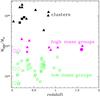 |
Fig. 1 Total mass (M200) versus redshift of the group and cluster samples. The low mass (poor) groups (6 × 10¹² < M200 < 6 × 10¹³ M⊙) are identified by the green symbols. The high mass (rich) groups (6 × 10¹³ < M200 < 2 × 10¹⁴ M⊙) are identified by the magenta symbols. Black symbols show the sample of clusters, all with M200 > 2 × 10¹⁴ M⊙. The stacked groups of Guo et al. (2014) are shown with a empty circles. The stacked clusters of Haines et al. (2013) are shown with filled squares. The high redshift group of Smail et al. (2014) is shown with a filled point. Green stars and filled magenta triangles show the low mass and high mass groups of Popesso et al. (2015), respectively. Filled black triangles show the cluster sample of Popesso et al. (2012) with the addition of the Coma cluster of Bai et al. (2006). The typical error of M200 for the low and high mass group samples is on the order of 0.2 dex, so much smaller than the M200 bin size considered in this analysis. The typical error of the bright clusters is on the order of 10% in the totality of the cases. |
2.1. Bolometric IR luminosity
For all groups in the sample of Popesso et al. (2015), the membership of their galaxies is available. For the galaxy members observed either by Herschel PACS or by Spitzer MIPS, we compute the IR luminosities by integrating the spectral energy distribution (SED) templates from Elbaz et al. (2011) in the range 8−1000 μm. The PACS (70, 100, and 160 μm) fluxes, when available, together with the 24 μm fluxes, are used to find the best fit templates among the main sequence (MS) and SB (Elbaz et al. 2011) templates. When only the 24 μm flux is available for undetected PACS sources, we rely only on this single point and use the MS template for extrapolating the LIR. Indeed, the MS template turns out to be the best fit template in the majority of the cases (80%) with common PACS and 24 μm detection (see Ziparo et al. 2013, for a more detailed discussion). In principle, the use of the MS template could only cause an underestimation of the extrapolated LIR from 24 μm fluxes, in particular at high redshift or for off-sequence sources due to the higher PAHs emission of the MS template (Elbaz et al. 2011; Nordon et al. 2010). However, as shown in Ziparo et al. (2013), the comparison between the LIR estimated with the best fit templates based on PACS and 24 μm data and the LIR extrapolated from 24 μm flux with only the MS template ( ) shows that the two estimates are in very good agreement, with only a slight discrepancy (10%) at z ≥ 1.7 or at
  .
.
3. Estimate of the total SFR and SFR/M
In this work we have defined the total SFR of a galaxy system (Σ(SFR)) as the sum of the SFR of its galaxy members with LIR down to 107 L⊙. The total SFR per unit of halo mass is defined as the Σ(SFR) divided by the total mass of the galaxy system. We explain here how these quantities are estimated for the different halo subsamples.
For the Popesso et al. (2012, 2015) group and cluster samples, the IR emitting – spectroscopically identified – galaxy members are available. Thus, for the groups and clusters in this subsample, the total IR luminosity of each system is obtained by summing up the LIR of the members within the system r200 and down to the LIR limit (LIR,limit) which corresponds to the 5σ flux level (flimit) of the deepest IR band, which is Spitzer MIPS 24 μm for all the groups of Popesso et al. (2015) and Herschel PACS 100 μm for several clusters of Popesso et al. (2012; see also Popesso et al. 2015, for the details about the flux limits reached in different fields and in different bands). The total IR luminosity is then converted into a total SFR via the Kennicutt (1998) relation. In this conversion we assume that the IR flux is completely dominated by obscured SF and not by AGN activity also for the 5% AGNs identified as X-ray sources among the group galaxy members. Eighty-seven percent of these AGNs are bright IR emitting galaxies observed by PACS. Herschel studies of X-ray AGNs (Shao et al. 2010; Mullaney et al. 2012; Rosario et al. 2012) have demonstrated that in the vast majority of cases (i.e., >94%), the PACS flux densities are dominated by emission from the host galaxy and thus provide an uncontaminated view of their star formation activities. The flux at 24 μm of the remaining 13% of AGNs observed only by Spitzer could in principle be contaminated by the AGN emission. However, since these galaxies are faint IR sources that only represent the 0.65% of the group galaxy population studied in this work, we consider that their marginal contribution cannot affect our results. Consequently, we assume that the IR luminosity derived here has no significant contribution from AGNs and can be converted into the obscured total SFR density of group galaxy population.
We also correct Σ(SFR) for spectroscopic incompleteness by multiplying it by the ratio of the number of sources without and with spectroscopic redshift, with flux density higher than flimit and within 3 × r200 of the X-ray center of the system. The incompleteness correction is estimated within 3 × r200 rather than within r200 to increase the statistics and to have a more reliable estimate. This correction is based on the assumption that the spectroscopic selection function is not biased for or against group or cluster galaxies, as ensured by the very homogeneous spatial sampling of the various spectroscopic campaigns conducted in the considered fields (see Cooper et al. 2012, for ECDFS; Barger et al. 2008 for GOODS-N and Lilly et al. 2009 for COSMOS). The incompleteness correction factor ranges from 1.2 to 1.66. To extend Σ(SFR) down to LIR = 107 L⊙, we use the group and cluster IR LF. This is estimated for the groups in several redshift bins up to z ~ 1.6 in Popesso et al. (2015). For low redshift clusters, it is provided by Haines et al. (2010) for the intermediate redshift LoCuSS clusters in Haines et al. (2013), and for the high redshift clusters at 0.6 < z < 0.8 by Finn et al. (2010). For clusters outside the mentioned redshift bins, we use the IR LF of the closest redshift bin. The best fit LFs are estimated in a homogeneous way for all cases in Popesso et al. (2015). We use here the best fits obtained with the modified Schechter function of Saunders et al. (1990). The correction down to LIR = 107 L⊙ is estimated as the ratio between the integral of the group or cluster IR LF down to LIR = 107 L⊙ and the integral down to the LIR,limit of each system. The correction down to LIR = 107 L⊙ due to the extrapolation from the best fit IR LF of groups and clusters is limited to less than 10−20% in all cases. Indeed, for low redshift systems, Σ(SFR) is estimated down to very faint LIR and a very small correction is applied. At higher redshift, instead, as shown in Popesso et al. (2015) for the groups and in Haines et al. (2013) for the clusters, the bulk of the IR luminosity is provided by the LF bright end, and a marginal contribution is provided by galaxies at LIR < 1010 L⊙. Thus, even for high redshift groups and clusters, whose Σ(SFR) estimate is limited to the IR brightest members, the correction down to LIR = 107 L⊙ is small.
To test the reliability of our method, in particular of the spectroscopic incompleteness correction, we used the mock catalogs of the Millennium Simulation (Springel et al. 2005). Out of several mock catalogs created from the Millennium Simulation, we chose those of Kitzbichler & White (2007) based on the semi-analytical model of De Lucia et al. (2006). The former authors make mock observations of the artificial Universe by positioning a virtual observer at z ~ 0 and finding the galaxies that lie on his backward light cone. We select several mock light-cone catalogs and extract from those the following info for each galaxy: the friend of friend (FoF) identification number, to identify the galaxy member of the same group/cluster (same FoF ID), the DM halo virial mass that, according to De Lucia et al. (2006), is consistent with the mass calculated within r200, as in the observed sample, the SFR, and the redshift. We transformed the SFR into LIR by following the Kennicutt (1998) relation. We then used the MS template of Elbaz et al. (2011), redshifted to the galaxy redshift, to estimate the Spitzer MIPS 24 μm flux of each simulated galaxy. The SB template is not used because off-sequence galaxies are generally much less numerous than MS ones.
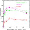 |
Fig. 2 Mean spectroscopic completeness in the Spitzer MIPS 24 μm band across the whole areas of the ECDFS, GOODS-N and COSMOS field (solid lines) and mean spectroscopic completeness simulated in the “incomplete” mock catalogs (dashed lines). |
To simulate the effects of the spectroscopic selection function of the surveys used in this work, we randomly extracted, as a function of the simulated MIPS 24 μm flux bin, a fraction of galaxies that is consistent with that of galaxies with available spectroscopic redshift in the same flux bin, observed in the GOODS and COSMOS surveys (see Fig. 2). Since the clusters of the Popesso et al. (2012) subsample are characterized by a spectroscopic completeness intermediate between the GOODS and COSMOS surveys, we limited this analysis to these surveys. We randomly extracted 25 catalogs for each survey from different light cones. The “incomplete” mock catalogs, produced in this way, tend to reproduce the biased selection, to a level that we consider sufficient for our needs, toward highly star-forming galaxies observed in the real galaxy samples (Fig. 2).
We then extracted a sample of galaxy groups and clusters in the same mass and redshift range as those of the observed sample from the original Kitzbichler & White (2007) mock catalogs. The members of the structures were identified by the same FoF identification number, defined according to the FoF algorithm described in De Lucia et al. (2006). We estimated the “true” Σ(SFR) as the one obtained by summing up the SFR of all members within r200. We limited this estimate down to 1010 L⊙ for all the structures as we cannot correct down to 107 L⊙ since the IR LF of groups in the mock catalog is not known and its determination is outside the scope of this paper. We point out that 1010 L⊙ is the average LIR,limit reached in our data set. We estimated the “observed” Σ(SFR) by summing up the member SFR of the same structures in the incomplete catalogs and by correcting for incompleteness by following the same procedure as applied in the real data set. Figure 3 shows the comparison of the “true” and “observed” quantities. We find fairly good agreement between the two values with a scatter about 0.2 dex. We used these simulations to estimate the error due to incompleteness in the Σ(SFR). This is estimated as the dispersion of the distributions of the residual Δ(SFR) = Σ(SFR)true − Σ(SFR)observed. This uncertainty varies as a function of the completeness level and of the number of group members. For a given completeness level, the lower the number of group members, the higher the uncertainty.
The total uncertainty of the Σ(SFR) estimates is determined from the propagation of error analysis by considering a 10% uncertainty in the LIRestimates (see Lutz et al. 2011, for further details) and the uncertainty due to the completeness correction. We did not consider the error of the correction down to 107 L⊙ since this correction is marginal.
For the Guo et al. (2014) stacked groups, we estimated the total IR luminosity in each redshift and halo mass bin by integrating the corresponding IR LF. As explained in Popesso et al. (2015), Guo et al. (2014) provide the Herschel SPIRE 250 μm LF, which must be converted into a total IR LF. For this purpose we used Eq. (2) of Guo et al. (2014) to transform the group Lν(250 μm) LF into the group IR LF. For consistency with Popesso et al. (2015), we fit the total IR LF of the Guo et al. (2014) stacked groups with the modified Schechter function of Saunders et al. (1990). Owing to the very low statistics of the Guo et al. (2014) LF in the 0.3 < z < 0.4 redshift bin, we limited this analysis to the z < 0.3 groups. The total IR luminosity of each stacked group is obtained by integrating the best fit modified Schechter function down to 107 L⊙. This is, then, converted into the Σ(SFR) via the Kennicutt (1998) relation. The error in Σ(SFR) is obtained by propagating the error of the total IR luminosity, which is in turn obtained by marginalizing over the errors of the best fit parameters.
For the stacked LoCuSS clusters of Haines et al. (2013), we used a slightly different approach. For the three stacked clusters at 0.15 < z < 0.2, 0.2,z < 0.25, and 0.25 < z < 0.3,Haines et al. (2013) provide the Σ(SFR) obtained by integrating the cluster IR LF down to 1011 L⊙. This was done to compare the LoCuSS cluster Σ(SFR) with the results of Popesso et al. (2012), where the Σ(SFR) estimate was limited to the LIRG population. We used the best fit of the IR LF of Haines et al. (2013) obtained by Popesso et al. (2015) to correct this quantity down to 107 L⊙. The error in the Σ(SFR) is obtained by summing in quadrature the errors of the estimates provided by Haines et al. (2013) and the error of the correction that is obtained by marginalizing over the errors of the best fit parameters. The Σ(SFR) of the Coma cluster is obtained by integrating the IR LF of Bai et al. (2006) down to 107 L⊙. Also in this case the error is obtained by marginalizing over the errors of the best fit parameters.
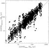 |
Fig. 3 “Observed” vs. “true” values of total SFR in the mock catalogs of Kitzbichler & White (2007). |
The IR LF of the Kurk et al. (2008) structure is studied in Popesso et al. (2015). We integrate this LF down to 107 L⊙ to obtain the total IR luminosity of the structure, hence its Σ(SFR) via the Kennicutt (1998) relation. Also in this case the error is estimated by marginalizing over the errors of the best fit parameters. For Cl 0218.3−0510, Smail et al. (2014) provide the Σ(SFR) obtained by summing up the contribution of the LIRGs in the structure. Also in this case this was done to compare with the results of Popesso et al. (2012). We used the IR LF of the Kurk et al. (2008) structure at the same redshift to correct the estimate of Smail et al. (2014) for the contribution of galaxies with IR luminosity in the 107−1011 L⊙ range. The error in the Σ(SFR) is obtained by summing in quadrature the errors of the estimates provided by Smail et al. (2014) and the error of the correction.
We finally defined the total SFR per unit halo mass () as the ratio of Σ(SFR) and the dynamical mass of the system within r200, M200. The error is estimated by propagating the error on Σ(SFR) and the error on the mass. By also taking the error due to the incompleteness correction applied to the Σ(SFR), we find that the accuracy of the estimate is ~0.25−0.3 dex.
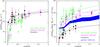 |
Fig. 4 Left panel: Σ(SFR)-redshift relation for low mass groups (green symbols), massive groups (magenta symbols), and clusters (black symbols) up to redshift ~1.6. The group and cluster sample of Popesso et al. (2012, 2015) are shown with triangles. The stacked groups of Guo et al. (2014) are shown with empty circles. The stacked clusters of Haines et al. (2013) and the Coma cluster of Bai et al. (2006) are indicated with filled squares. The Kurk et al. (2008) group is shown with a triangle, while the Smail et al. (2014) structure is shown with a filled circle. The green, magenta, and black solid lines show the low mass group, massive group, and cluster best fit relation of the form Σ(SFR)∝ zα, respectively. Right panel: -redshift relation for the same sample. The color coding and the symbols have the same meaning as in the left panel. The overall -redshift relation is derived from Magnelli et al. (2013) and is shown by the blue shaded region. The shading represents 1σ confidence levels as reported in Magnelli et al. (2013). This region is moved 0.4 dex up (two dashed blue lines) to indicate its locus under the assumption that not all the mass in the considered volume is locked in halos, as claimed by Faltenbacher et al. (2010). |
4. The total SFR per halo mass versus redshift
In Fig. 4 we show the Σ(SFR)-z (left panel) and the (right panel) relations for the systems considered in this work. As explained in Sect. 2, we distinguish the galaxy systems in low mass and high mass groups and clusters, depending on their total mass. We also show the overall relation. This overall relation is obtained by dividing the observed star formation rate density (SFRD) of Magnelli et al. (2013), by the mean comoving density of the Universe (Ωm × ρc where Ωm = 0.3 and ρc is the critical density of the Universe). The SFRD has been evaluated by integrating the overall IR LF of Magnelli et al. (2013) based on PACS data, down to LIR = 107/L⊙ and by converting the integrated IR luminosity into a total SFR via the Kennicutt (1998) relation in each redshift slice. The overall SFRD has been estimated in large comoving volumes that include galaxy systems, voids, and isolated galaxies, and is thus representative of the overall galaxy population. We point out, however, that the for the overall population is only a lower limit. Indeed, not all the mass is locked in halos that host galaxies. As shown in Faltenbacher et al. (2010), the fraction of mass locked in halos also depends on the local density field. Thus, using the mean comoving density of the Universe can lead to underestimating the for the overall galaxy population. Following Faltenbacher et al. (2010) this underestimation should be ≤ 0.4 dex. In the righthand panel of Fig. 4, we move the overall relation upward by 0.4 dex to show where it should lie under the assumption that not all the mass is locked in DM halos.
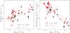 |
Fig. 5 Σ(SFR)-mass relation in two redshift slices, 0.2 < z < 0.5 (red points) and 0.5 < z < 1 (black points) of Fig. 4. The solid lines show the best fit relations. -mass relation in two redshift slices, 0.2 < z < 0.5 (red points) and 0.5 < z < 1 (black points) of Fig. 4. The solid lines show the best fit relations. |
We fit both the Σ(SFR)− z and the relations with a power law. The best fits in the three mass bins for the Σ(SFR) − z relation are, for clusters, 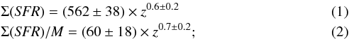 for massive groups,
 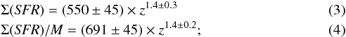 and for low mass groups,
 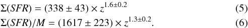 The Σ(SFR)− z is much noisier than the relation. The power law fit is poorly constrained in the Σ(SFR)− z relation, while it provides a very good fit for the relation. The total SFR appears to be fairly similar in all structures independently of the redshift. Clusters are in general much richer in number of galaxies with respect to low mass groups, so that their total SFR is on average higher (0.2−0.3 dex, 1−1.5σ) than in the low mass systems. Indeed, if we zoom into a redshift slice, as shown for instance in the lefthand panel of Fig. 5, we observe a rather flat, though clear, positive correlation between the total SFR and the system mass (Σ(SFR)∝ M0.2 at 0.2 < z < 0.5 and Σ(SFR)∝ M0.35 at 0.5 < z < 1). Since the number of galaxies is increasing linearly with the halo mass, as shown by Yang et al. (2007) in the local Universe and more recently by Erfanianfar et al. (in prep.) up to z ~ 1, it follows that at least up to z ~ 1, the mean SFR is higher in the low mass systems than in clusters.
Once the Σ(SFR) is normalized to the halo mass, the situation reverses, and the low mass groups appear to be more active per unit mass than their high mass counterparts. Indeed, as shown in the righthand panel of Fig. 4, the low mass groups show a mean activity per unit mass more than one order of magnitude higher with respect to the clusters. The figure thus indicates a clear anti-correlation between and the system mass at any redshift. The relation exhibits a higher significance with respect to the Σ(SFR) − M200 relation and lower scatter, as shown in the righthand panel of Fig. 5. We point out that we do not find a faster evolution (steeper relation) in more massive systems, unlike in Popesso et al. (2012). However, at variance with Popesso et al. (2012) we consider here the overall IR emitting population by integrating the system IR LF, while Popesso et al. (2012) only considered the evolution of the LIRG population. In Popesso et al. (2015) we show that the LIRG population is evolving in a much faster way in massive systems, and this could be the cause of the apparent inconsistency with our previous results. In addition, we also split groups into two subsamples here, and we have to pay the price of having poorer statistics, hence larger errors, in the best fit parameters.
Lower mass groups appear to lie above the overall relation, something that was not noted in our previous analysis (Popesso et al. 2012). A lot of star formation activity is therefore occurring in the small volume occupied by the numerous group-sized DM halos. More massive groups tend to have SF activity per halo mass that is consistent with the overall relation, even if we account for an underestimation of the overall of 0.4 dex (Faltenbacher et al. 2010). Star formation activity is largely suppressed in the most massive, cluster-size halos at any redshift.
To take full advantage of the redshift and dynamical range covered by our sample, we also fit the plane. The best fit turns out to have the form  (7)The scatter around the plane is 0.35 dex, which is slightly greater than the accuracy in our estimate of the , which, according to our simulation (see Sect. 3), is 0.25−0.3 dex. We point out that, while for the relation in the individual mass bin, a power law of the form provides the best fit in all cases, a redshift dependence of the kind provides a slightly better fit to the plane. Indeed, the final scatter around the plane decreases from 0.42 dex to 0.35 dex as shown in Fig. 6. We also tried to adopt the same approach for the Σ(SFR) − z − M200 plane, but the large scatter observed in the Σ(SFR) − z relation also generates a large scatter in the plane.
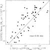 |
Fig. 6 Residual of the observed with respect to the best fit plane . |
5. The cosmic star formation rate density of massive halos
To understand what the contribution of DM halos is for different masses to the evolution of the cosmic SFRD (ρSFR), we use the best fit plane with the following procedure. Since Σ(SFR)is a monotonically increasing function of M200 (see left panel of Fig. 5), we use the lower and upper limit of each mass range to retrieve the corresponding lower and upper limit of the Σ(SFR) − z relation by fixing the value of M200 in the plane. We prefer this approach rather than using directly the fitted Σ(SFR)− z − M200 plane and the Σ(SFR)− z relation because, as discussed in previous section, the larger noise of these correlations leads to a poorer fit than for the plane. To transform the Σ(SFR) − z regions identified for each mass bin into a SFR density as a function of redshift, we multiply each of them for the comoving number density of DM halos in the corresponding mass range as a function of redshift (ρNhalo(z)). This quantity is estimated by using the WMAP9 concordance model prediction of the comoving ρNhalo(z) of halos in the three mass ranges. This model reproduces the observed log (N) − log (S) distribution of the deepest X-ray group and cluster surveys (see, e.g., Finoguenov et al. 2010). The evolution of ρNhalo as a function of redshift in each mass range is shown in Fig. 7. For comparison we also estimate the comoving ρNhalo(z) in the same mass bins according to the Planck cosmology based on the SZ Planck number counts (Planck Collaboration XX 2014,Fig. 7). In this cosmology, the number of clusters and groups is higher by 0.15, 0.18, and 0.25 dex, on average, up to z ~ 1.5 for low mass, high mass groups, and clusters, respectively.
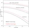 |
Fig. 7 Comoving density of the DM halos as a function of redshift (ρNhalo(z)) in the three M200 mass ranges considered in this work according to the WMAP9 (black solid curves) and Planck (red dashed curves) cosmologies. |
Figure 8 shows the contribution of each halo mass range to ρSFR(z). In calculating these contributions, we include an error of 0.35 dex in the derived from the as explained in Sect. 4. The shaded blue region shows the overall evolution of obscured ρSFR in all halo masses as derived by Magnelli et al. (2013). THey combine the obscured ρSFR with the unobscured ρSFR derived by Cucciati et al. (2012) using rest-frame UV observations. However, we do not know the contribution of the unobscured SFRD for the group galaxy population. Thus, for a fair comparison we only considered the contribution of the group galaxy population to the obscured ρSFR, as also done in Popesso et al. (2015). We point out, however, that the obscured ρSFR dominates the total ρSFR at any redshift. Indeed, Magnelli et al. (2013) report that the unobscured ρSFR only accounts for about s25%, s12%, and s17% of the total ρSFR at zs0, zs1, and zs2, respectively. In addition, there are no reasons to assume that the same correction could be applied to the group galaxy SFRD, since it is not known whether the evolution of the mean rest-frame UV dust attenuation depends on environment. For completeness we also overplotted the compilation of values from Hopkins & Beacom (2006), which have also been derived from UV data.
Figure 8 goes on to show that the contribution of low mass groups (masses in the range 6 × 10¹²−6 × 10¹³ M⊙) provides a substantial contribution (50−80%) to the ρSFR at z ~ 1. Such a contribution declines faster than the cosmic ρSFR between redshift 1 to the present epoch, reaching a value of <10% at z < 0.3. This is consistent with our findings of Popesso et al. (2015) based purely on the integration of the IR LF of group galaxies in four redshift intervals up to z ~ 1.6.
More massive systems, such as high mass groups and clusters, only provide a marginal contribution (<10% and <1%, respectively) at any epoch. This is for two reasons: 1) they show in general a much lower SF activity per halo mass than less massive systems and 2) their number density is, especially at high redshift, orders of magnitude lower that the one for low mass groups (see Fig. 7). In particular, the number density of clusters is extremely low at z > 1 since these massive structures are created at more recent epochs. Thus, their contribution declines at z > 1.
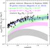 |
Fig. 8 Contribution of each halo mass range to the CSFH as a function of redshift. The CSFH of the Universe is taken from Magnelli et al. (2013). The shading indicates the 1σ confidence level as derived in Magnelli et al. (2013). The shaded green, magenta, and black regions show the contributions of the low mass group, high mass group, and cluster galaxy populations, respectively. The black points show the compilation of Hopkins & Beacom (2006). |
Since halos of masses higher than ~6 × 10¹² provide a negligible contribution to the cosmic ρSFR at z < 0.3, it follows that this must be sustained by galaxies in lower mass halos. This is consistent with the findings of Heavens et al. (2004), Gruppioni et al. (2013,the former based on the SDSS fossil record, the latter entirely based on Herschel that the most recent epoch of the CSFH is dominated by galaxies of low stellar masses (M⋆ < 108−9 M⊙), which most likely inhabit very low mass halos.
We would like to point out that using the Planck cosmology would not change these conclusions.
5.1. An alternative approach
To understand the physical implications of the result shown in Fig. 8, we use an alternative method. If the galaxies belonging to low mass groups provide a substantial contribution to ρSFR at z ~ 1 and beyond, it means that at this epoch there must be a significant fraction of the whole galaxy population. Our data set does not allow us to check this possibility, since at the moment we do not have a complete census of the galaxy population in terms of their parent DM halo mass owing to the lack of sufficient spectroscopic information.
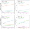 |
Fig. 9 Fraction of galaxies belonging to parent halos of different masses. Each panel shows a different stellar mass range: M⋆/M⊙ = 109−1010upper left, 1010−1010.5upper right, 1010.5−1011bottom left, and >1011bottom right. Different colors label different parent halo masses, as indicated in each panel. |
To overcome this problem, we use the predictions of the most recent simulations to associate galaxies of a given stellar mass to their parent halo and the observational results to match stellar mass and SF activity. We favor, in particular, the most recent Guo et al. (2013) model since it makes use of the more recent WMAP7 cosmology rather than the WMAP1 cosmology still adopted by Kitzbichler & White. (2007). The most significant difference between the cosmologies preferred by WMAP7 and WMAP1 data is a 10% lower value of σ8. This implies a lower amplitude for primordial density fluctuations, which translates into a decrease in the number of halos with masses above M∗ and an increase for those below this characteristic mass. Thus, the model of Guo et al. (2013) reproduces the clustering properties of the galaxy population of the local Universe and the evolution of the galaxy stellar mass function up to high redshift fairly well. For this reason we used this simulation to match the galaxy stellar mass to the parent halo mass.
We use the galaxy catalogs of this model with the following approach. We define four stellar mass ranges (log (M⋆/M⊙) = 9−10, 10−10.5, 10.5−11, and >11) and estimate, in each range, the fraction of galaxies belonging to parent halos of different mass ranges (M200/M⊙ = 1011−1012, 1012−6 × 10¹², 6 × 10¹²−6 × 10¹³, 6 × 10¹³−2 × 10¹⁴, >2 × 10¹⁴). Figure 9 shows the redshift evolution of these fractions and, thus, the halo mass range that dominates in each stellar mass range. Halos with masses corresponding to the low mass groups analyzed in this paper (in the range 6 × 10¹²−6 × 10¹³ M⊙) dominate only at M⋆ > 1011 M⊙, and only at z > 1. More massive halos only host a marginal fraction <10% of the whole galaxy population at any stellar mass.
However, the Guo et al. (2013) model shares the same problems of previous models with respect to the level of galaxy SF activity. As discussed in more detail in next section, this model also underpredicts the galaxy SFR as a function of M⋆ at any epoch. Thus, to link the galaxy M⋆ to the SFR, we use real data and, in particular, to the observed SFR-M⋆ plane. In particular, we use the photometric COSMOS Spitzer and PACS galaxy catalog matched to the Ilbert et al. (2010) photometric redshift and M⋆ catalog. We must limit our analysis to the LIRG regime at IR luminosities higher than 1011 L⊙ (SFR > 17 M⊙/ yr according to the Kennicutt relation 1998) and to M⋆ > 109 M⊙ to ensure the highest photometric completeness at least up to z ~ 1−1.2 (see Ilbert et al. 2010; Magnelli et al. 2011, for a complete discussion about completeness).
In any redshift bin, we divide the LIRG region of the SFR-M⋆ plane into four regions according to the M⋆ bins defined above (see, e.g., Fig. 10). Given the completeness of the sample, we can calculate the fraction of total SFR due to each M⋆ bin with respect to the total SFR of the whole LIRG population. This is done in several redshift bins.
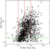 |
Fig. 10 Example of the SFR-stellar mass plane at z ~ 0.5 drawn from the COSMOS Spitzer and PACS galaxy catalog matched to the Ilbert et al. (2010) photometric redshift and stellar mass catalog. For any redshift bin, we divide the LIRG region of the SFR-stellar mass plane (SFR > 17 M⊙/ yr, above the green solid line) in four regions (red solid lines) according to the stellar mass bins defined in the text. |
We combine these different estimates to calculate the fraction of the total SFR due to each DM halo mass range limited to the LIRG population in the following way: 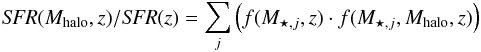 (8)where SFR(Mhalo,z)/SFR(z) is the fraction of the total SFR due to the LIRG population of galaxies per halo mass (Mhalo) at the redshift z, f(M⋆,j,z) is the fraction of the total SFR due to the LIRGs in the jth stellar mass bin at redshift z, and f(M⋆,j,Mhalo,z) is the fraction of galaxies in the jth stellar mass bin at redshift z and belonging to DM halos of mass Mhalo. The sum is done over the stellar mass ranges in a given redshift bin. We use this fractional contributions to estimate the ρSFR(z) per halo mass in the Magnelli et al. (2013)ρSFR(z) limited to the LIRGs; namely, we multiply the Magnelli et al. (2013)ρSFR(z) by these fractional contributions.
The main limit of this approach is that it does not take gradients along the MS as a function of the halo mass into account. In other words, this method does not consider that galaxies in massive halos could favor the regions below the SF galaxy MS, in particular at low redshift, as shown for instance in Bai et al. (2009) and Ziparo et al. (2013). In the same way this model does not take into account that at high redshift there should be a reversal of the SFR-density relation at the epoch when massive galaxies at the center of groups and clusters form the bulk of their stellar population in strong bursts of SF activity, as predicted by models (e.g., De Lucia et al. 2006). In other words we assume that the galaxy SFR distribution is independent of the halo mass at any redshift. Nevertheless, we consider that in a first approximation, this method still provide a valuable way to check the robustness of our results.
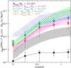 |
Fig. 11 CSFH per halo mass limited to the LIRG population. The shaded regions are the CSFH per halo mass as in the left panel of Fig. 8. The points are the contributions per halo mass as estimated in the current analysis. Colors indicate different halo mass ranges as indicated in the figure. |
The results are shown in Fig. 11. The blue shaded region is the overall CSFH of Magnelli et al. (2013) limited to the LIRG population. This is obtained by integrating the overall IR LF of Magnelli et al. (2013) down to LIR = 1011 L⊙. The green, magenta and black shaded regions are the contributions of low mass, massive groups and clusters, respectively, to the overall LIRG CSFH. These are estimated in a similar way as described in previous section; that is to say, we fit the plane by limiting the estimate of the to the LIRG population. The best fit relation  (9)is used in the same way as described in the previous section to retrieve the contribution to the CSFH of the galaxy population inhabiting DM halos of different masses. We point out that the evolution of the with redshift limited to the LIRG population is much steeper than the relation obtained for the whole IR-emitting galaxies. This is consistent with the faster evolution of the LIRG number and luminosity density observed already in the overall population (Magnelli et al. 2013; Gruppioni et al. 2013) and in the same sample of galaxy groups in Popesso et al. (2015). The halo mass dependence of the LIRG is, instead, quite consistent with the one of the whole IR-emitting group galaxy population. The scatter around the best fit plane of the LIRG population is 0.35 dex as for the previous case.
The points in Fig. 11 are the contributions per halo mass as estimated in this analysis. There is an overall good agreement for the low mass groups (green points and shaded region) and for the massive groups (magenta points and shaded region). There is no agreement for the cluster mass range, but it is rather difficult to judge whether the problem is in the data due to the low number statistics in the cluster mass regime or in the models since there are not so many massive clusters in the Millennium Simulation due to the limited volume. We also plot the relation obtained for the halo mass ranges not covered by our group sample at 1012 < Mhalo/M⊙ < 6 × 10¹² (cyan points) and Mhalo/M⊙ < 1012 (orange points).
Figure 11 leads to the following conclusions. The main contributors to the CSFH, at least for the LIRG population, are low mass groups in the ranges 1012 < Mhalo/M⊙ < 6 × 10¹² and 6 × 10¹² < Mhalo/M⊙ < 6 × 10¹³ that, together, account for 60-70% of the CSFH at any redshift up to z ~ 1.2. The main reason for this is mass segregation. Indeed, as shown in the panels of Fig. 9, these groups contain the largest fraction of massive galaxies at M⋆ > 1010.5−1011 M⊙, which have strong SF along the MS. The more massive groups and the clusters are relatively rare objects, and they only host only a marginal fraction of the galaxy population at any mass, thus their contribution to the CSFH is quite small. The DM halos in the lowest mass range at Mhalo/M⊙ < 1012 host the majority of the low mass galaxies, which are extremely numerous but have a very low SFR, according to their low mass. Thus, these halos also provide a marginal contribution to the CSFH. If we could extend our analysis to the whole star-forming galaxy population rather than purely the LIRG, we would very likely see these halos dominating the current epoch of the CSFH, since according to Heavens et al. (2004) and Gruppioni et at (2013), low mass galaxies are the dominant star-forming galaxy population in the local Universe.
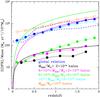 |
Fig. 12 -redshift relation obtained from the semi-analytical model of De Lucia et al. (2006) applied to the Millennium simulation (filled and empty points). Different colors correspond to halos of different masses, as indicated in the figure. The region contained within the dashed blue line indicates the overall relation obtained from the overall SFR density evolution of Magnelli et al. (2013) as shown in the right panel of Fig. 4. We plot here the overall -redshift relation that considered that not all the mass is locked in halos. The solid lines show the observed best fit -redshift relations shown in the right panel of Fig. 4. |
6. Comparison with models
We compare here our results with several models available in the literature in order to test their predictions.
6.1. Semi-analytical models
As a first approach we use the Millennium simulation (Springel et al. 2005), which is publicly available, to perform the same analysis as for our real data set directly on the simulated data sets. We test here the predictions of the simulated data sets provided by different semi-analytical models available in the Millennium database (De Lucia et al. 2006; Bower et al. 2006; Kitzbichler & White 2007; Guo et al. 2011).
Figure 12 shows the -redshift relation for different halo mass ranges based in particular on the De Lucia et al. (2006) model. We used M200 as an estimate of the total mass of DM halos in the simulation because it is calculated in a consistent way with respect to the observations. As in the observed data set, we estimate the Σ(SFR)of each halo as the sum of all members, identified with the same ID number by the FoF algorithm applied by De Lucia et al. (2006) and within r200 of the central galaxies (identified as a type = 0 galaxy in the Millennium database).
Figure 12 shows that the overall -redshift relation (blue points) agreems with the observations if we consider that not all the mass is locked in halos and if we correct the overall relation obtained from the CSFH of Magnelli et al. (2013) by 0.4 dex, as derived by using the results of Faltenbacher et al. (2010). Nevertheless, the analysis of the -redshift relation in different halo mass ranges shows that the model of De Lucia et al. (2006) strongly underpredicts the mean level of activity per halo mass of all massive halos in the same range as considered in this work. According to the model the galaxy population of halos with masses above 6 × 10¹² M⊙ lie more than one order of magnitude below the general relation and showing a discrepancy of more than two orders of magnitude with respect to the observations.
The models of Bower et al. (2006) and Guo et al. (2011) lead to very similar results despite some marginal quantitative differences. Indeed, the models of galaxy evolution available in the Millennium database (De Lucia et al. 2006; Bower et al. 2006; Kitzbichler & White 2007; Guo et al. 2011) all predict a faster than observed evolution of galaxies in massive halos. This class of models assumes that, when galaxies are accreted into a more massive system, the associated hot gas reservoir is stripped instantaneously. This, in addition to the AGN feedback, induces a very rapid decline of the star formation histories of satellite and central galaxies, respectively, and contributes to create an excess of red and passive galaxies with respect to the observations (Wang et al. 2007). This is known as the “over-quenching problem” for satellites galaxies. Over 95% of the cluster and group galaxies within the virial radius in the local simulated Universe are passive (Guo et al. 2011), at odds with observations (Hansen et al. 2009; Popesso et al. 2005). The first consequence is that the predicted CSFH is too low in comparison to to observations, and it does not show the observed plateau between redshift 1 and 2, but a peak at z ~ 2 and a rapid decline afterward (see Fig. 9 in Kitzbichler & White 2007). The second consequence is that the contribution of group and cluster galaxies to the CSFH is always negligible since the SF is immediately quenched (see Fig. 13). The SFR density at any epoch is dominated by the activity of galaxies in low mass halos (Mhalo < 1012 M⊙). Moreover, according to De Lucia et al. (2012) group galaxies are quenched at early epochs, even before they enter the cluster environment (the preprocessing scenario, see Zabludoff & Mulchaey 1998). This is at odds with the much higher level of SF activity in low and high mass groups at any redshift with respect to the clusters, as shown in the lefthand panel of Fig. 4.
Despite the use of the WMAP7 cosmology, which shifts the peak in cosmic SFR to lower redshift, the Guo et al. (2013) model also leads qualitatively to the same results of Figs. 12 and 13 based on De Lucia et al. (2006) model. The results based on the Millennium simulation also qualitatively agree with the van de Voort et al. (2011) model, based on a completely different set of simulations, which find that DM halos with masses above 1013 M⊙ do not contribute at all to the CSFH of the Universe.
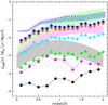 |
Fig. 13 Contribution of halos of different mass to the CSFH as obtained from the semi-analytical model of De Lucia et al. (2006) applied to the Millennium simulation (filled points). Different colors correspond to halos of different masses. The color coding is the same as in Fig. 12. The shaded green, magenta, and black regions show the observed contribution of low mass group, massive group, and cluster, galaxy population, respectively to the overall relation of Magnelli et al. (2013, blue shaded region). |
6.2. Abundance matching methods
As an alternative to semi-analytical models, models using the merger trees of hydrodynamical simulations and a conventional abundance-matching method to associate galaxies to DM halos are often used to study the mass accretion history of galaxies as a function of their parent halo mass (e.g., Vale & Ostriker 2004; Conroy & Wechsler 2009; Behroozi et al. 2010). It is rather instructive to compare three of these models, which are quite similar in concept, but rather different in their treatment of the mass accretion of satellite galaxies after they enter a massive halo.
The Moster et al. (2013) multi-epoch abundance matching (MEAM) model employs a redshift-dependent parametrization of the stellar-to-halo mass relation to populate halos and subhalos in the Millennium simulations with galaxies, requiring that the observed stellar mass functions at several redshifts be reproduced simultaneously. Interestingly, the model assumes that the stellar mass of a satellite does not change after its subhalo entered the main halo; i.e., it neglects stellar stripping and star formation in the satellites. Thus, by construction this model implements the same “satellite over-quenching” as observed in the Millennium simulation. In other words, the star formation activity of any halo is only located in its central galaxy. Moster et al. (2013) provide useful fitting functions to estimate the redshift evolution of the SFR of a DM halo of a given mass at redshift close to zero. Figure 14 shows the comparison between our estimate of the Σ(SFR)-redshift relation with the evolution of the Σ(SFR) in halos of similar mass at redshift ~0. The comparison is not completely straightforward because the halo mass also evolves with redshift according to the DM halo accretion history. However, according to Moster et al. (2013) a typical massive halo of Mhalo = 1014 M⊙ at z ~ 0 has grown from a z ~ 1 halo with a virial mass of Mhalo = 1013.6 M⊙, while lower mass halos accrete even less in the same amount of time. Thus, the considered massive systems at z ~ 0 remain in the same halo mass bin for most of the time window considered here. As expected, the “satellite over-quenching” implemented in the model provides results that are consistent with the semi-analytical model, underpredicting the relative contribution of DM halos of different masses to the CSFH. Interestingly enough, the model is anyhow able to reproduce the evolution of the galaxy stellar mass function and the overall CSFH.
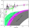 |
Fig. 14 Σ(SFR)-redshift relation obtained from the MEAM model of Moster et al. (2013). The symbols and solid lines in the figure have the same meaning as in the left panel of Fig. 4. The shaded regions indicate the evolution of the SFR in DM halos with mass at redshift ~0 in the range 6 × 10¹² < Mhalo/M⊙ < 6 × 10¹³ (light green), 6 × 10¹³ < Mhalo/M⊙ < 2 × 10¹⁴ (light magenta), and Mhalo/M⊙ > 2 × 10¹⁴ (gray). |
Unlike Moster et al. (2013), Yang et al. (2012) assume that a galaxy after becoming a satellite can gain stellar mass due to SF and suffer mass loss due to passive evolution. The satellite evolution is modeled as 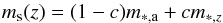 (10)where ms(z) is the satellite stellar mass at redshift z, m∗ ,a is the mass of the satellite at the accretion time, and m∗ ,z the expected median stellar mass of central galaxies in halos of the same mass of the satellite subhalo at redshift z. For c = 0 the satellite does not increase the mass after accretion into the host halo as in Moster et al. (2013). Instead, for c = 1 the satellite accretes stellar mass in the same way as a central galaxy of equal mass. The c parameter is left free in the fitting. In addition to the consistency with the evolution of the galaxy stellar mass function, the best fit model is required to also reproduce the local conditional galaxy stellar mass function (as a function of the halo mass) of Yang et al. (2007) and the two-point correlation function of SDSS galaxies. The best fit value is c = 0.98, implying that satellites accrete considerable mass after accretion, similar to the central galaxies of similar halos. According to the stellar mass assembly histories of Yang et al. (2012), the mass increase of such galaxies is dominated by in situ SF rather than accretion, until the halo reaches a mass of ~1012 M⊙. This feature seems to hold independently of the final host halo mass of the central galaxy. Thus, satellite in subhalos with masses below ~1012 M⊙ should considerably contribute to the overall SF activity of massive halos. Unfortunately, Yang et al. (2012) do not provide predictions for the SF history of galaxies as a function of the host halo. Thus, a quantitative comparison with our results is not possible, though the qualitative predictions could lead to better consistency with our observations.
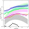 |
Fig. 15 Contribution of halos of different mass to the CSFH as obtained from the abundance-matching model of Bethermin et al. (2013, filled points). The color coding is the same adopted in Fig. 13. The shaded green, magenta, and black regions show the observed contribution of low mass group, massive group, and cluster, galaxy population, respectively, to the overall relation of Magnelli et al. (2013, blue shaded region). |
A step forward is made in the model of Béthermin et al. (2013), who use the stellar mass function of star-forming galaxies and passive galaxies of Ilbert et al. (2010) and the halo mass function of Tinker et al. (2008) to populate the nth most massive halo with the nth most massive galaxy by taking an increasing fraction of passive galaxies into account as a function of the galaxy stellar mass. Since more massive galaxies inhabit more massive halos, this leads naturally to a higher fraction of passive galaxies in massive halos. The link between stellar mass and SF activity as a function of time is done by considering the evolution of the MS of SF galaxies. The Elbaz et al. (2011) SED templates for MS and SB galaxies are used to estimate the mean IR emissivity of the galaxy population of a given halo. The model for the emissivity takes a satellite quenching into account that is modeled as a function of the satellite stellar mass (mass quenching) or as a function of the host halo mass (environment quenching). The free parameters are constrained by requiring the fit of the power spectra of the cosmic infrared background (CIB), the cross-correlation between CIB and cosmic microwave background lensing, and the correlation functions of bright, resolved IR galaxies. Though the model with the environment quenching agrees more closely with the observational constraints, the mass quenching also provide a reasonable fit. Béthermin et al. (2013) use the best fit model to predict the contribution of halos in different mass ranges to the CSFH.
Figure 15 shows the comparison between the Béthermin et al. (2013) best model and our results. With respect to the semi-analytical models and the Moster et al. (2013) models, the lack of the immediate suppression of the satellite SF activity after the accretion into the host halo, moves the bulk of the SF from very low mass halos (Mhalo < 1012 M⊙) to more massive halos (1012 < Mhalo/M⊙ < 1012.5 cyan points, and 1012.5 < Mhalo/M⊙ < 1013.5 green points), which agrees much more with our results and, in particular, with the results based on our alternative method (see Sect. 5.1). The green curve, in particular, which shows the contribution of halos in a mass range that is quite consistent with our low mass groups is consistent with our result between 0.3 < z < 1.3. At lower redshift the SF activity is predicted to be much higher than the observations, while at higher redshift the SFR density of galaxies in such halos is underpredicted with respect to the green shaded region, which at this redshift is, however, just an extrapolation from our best fit Σ(SFR) − M200-redshift relation. The prediction of the contribution of halos in a mass range consistent with out massive groups is consistent with the observations only up to z ~ 0.8. Beyond this redshift the magenta curve is far below the shaded region of the same color. For clusters, instead, the prediction is largely underestimated. We point out that the discrepancy could arise from constraining the fraction of quenched galaxies with the galaxy stellar mass functions of quenched and active galaxies of Ilbert et al. (2010), which are based on SED types only chosen among a few templates. The SED fitting technique provides a very poor constraint of the galaxy SF activity. Indeed, as shown by Ziparo et al. (2014), the SFR predicted by the SED technique correlates with the more accurate SFR derived from IR data with large scatter (0.6−0.7 dex).
6.3. Hydrodynamics simulations
A common feature of all previous models is that the relation between the central galaxy stellar mass and the halo mass reaches a maximum at halo masses ~1012 M⊙. According to Yang et al. (2012), below this threshold the mass accretion of the central galaxy is dominated by star formation. Thus, when the halo mass reaches ~1012 M⊙ a process takes place that quenches the star formation. Interestingly, this mass scale is very similar to the cold-mode to hot-mode transition scale (Birnboim & Dekel 2003; Kereš et al. 2005) in the theory of gas accretion, as derived in hydrodynamic simulations, whereas large halos primarily accrete hot gas and low mass halos cold gas. This would suggest that the quenching of central galaxies coincides with the formation of a hot gaseous halo, and thus with a lack of cold gas supply. What would be the fate of satellites? According to Simha et al. (2009), the subhalos also retain their identity for quite some time after accreting a larger halo, so satellites in subhalos less massive than ~1012 M⊙ do not immediately see the effect of the hot gas in the larger halo and accrete in cold mode. Thus, consistent with the results of Yang et al. (2012) and Béthermin et al. (2013), satellite galaxies continue to accrete gas and convert it to stars over a rather long period, which according to Simha et al. (2009) is about of 0.5−1 Gyr after the merger. The gas accretion declines steadily over this period. Since star formation follows mass accretion with a short delay, satellites should experience quenching in a similar amount of time. This scenario would be consistent with our observations. Indeed, at z ~ 1 when massive halos are just forming via merger, the SF activity in the accreted subhalos is still high. At later epochs, instead, the transition to the hot mode accretion of the satellites and the consequent progressive quenching of their SF activity would lead to the faster decline of their contribution to the CSFH with respect to lower mass halos, which evolve in a cold mode accretion phase maintaining a high SFR.
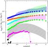 |
Fig. 16 Contribution of halos of different mass to the CSFH as obtained from the Illustris hydrodynamical simulation (Genel et al. 2014, filled points). The color coding of shaded regions and points is the same as adopted in Figs. 13 and 15. |
Figure 16 shows the comparison between our observations and the predictions of the Illustris hydrodynamical simulation Genel et al. (2014). The simulation still underpredicts the contribution of massive halos to the CSFH. However, the underestimation of such contribution is reduced with respect to the results of semi-analytical models. This holds, in particular, for halos in the low mass group range (geen shaded region and points in the Fig. 16). Indeed, for this class of halos, the observed and the predicted contributions to the CSFH agree up to z ~ 0.3 and differ by ~0.4 to 0.8 dex up to z ~ 1.5. Thus, a more physical treatment of the satellite quenching leads to an inprovement in the predictions if compared to the almost two orders-of-magnitude disagreement of the predictions of semi-analytical models (Fig. 13). However, we still see a large disagreement for more massive halos such as high mass groups (magenta shaded region and points) and clusters (black shaded region and points). We speculate that one possible explanation for such disagreement could be an oversuppression of the SF activity in the massive galaxies hosted by such halos due to “radio-mode” AGN feedback. This hypothesis is supported by the evidence that in the Illustris simulation, the redshift ~0 halos of ~1013 M⊙ are almost devoid of gas as a result of radio-mode AGN feedback, in disagreement with observations Genel et al. (2014).
Cen (2011) proposes that not only the halo mass, but also the halo environment on intermediate scales (~2 Mpc) could be a determinant of the gas accretion mode. The overall heating of cosmic gas due to the formation of large halos and large-scale structures causes a progressively greater fraction of halos to inhabit regions where the gas has an entropy that is too high to cool and continue feeding the galaxies. Thus, the lack of cold gas supply would affect not only halos above a given mass threshold but all halos inhabiting overdense regions. The effect is differential in that overdense regions are heated earlier and to higher temperatures than lower density regions at any given time. Because larger halos tend to reside in more overdense regions than smaller halos, the net differential effects would naturally lead to both the standard galaxy downsizing effect and the halo downsizing effect shown in Fig. 4.
7. Discussion and conclusions
The analysis of the -redshift relation in DM halos of different masses shows that low mass groups (halos with masses in the range 6 × 10¹²−6 × 10¹³ M⊙) lie well above the overall (mean) relation, showing that a lot of star formation activity is confined in a very small volume in the most common and numerous group-sized DM halos. More massive groups tend to have a SF activity per halo mass that is consistent with the overall relation, even if we account for an underestimation of the overall of 0.4 dex (Faltenbacher et al. 2010). Star formation activity is largely suppressed in the most massive, cluster-size, halos at any redshift.
The analysis of the contribution to the CSFH by halos in different mass ranges shows that low mass groups provide a 60−80% contribution to the ρSFR at z ~ 1. This contribution declines faster than the cosmic ρSFR between redshift 1 to the present epoch. This is consistent with our findings based purely on the integration of the IR LF of group galaxies in four redshift intervals up to z ~ 1.6 (Popesso et al. 2015). More massive systems, such as massive groups and clusters, only make a marginal contribution (<10% and <1%, respectively) at any epoch. Since halos of masses higher than ~6 × 10¹² M⊙ make a negligible contribution to the cosmic ρSFR at z < 0.3, it follows that this must be entirely contributed by galaxies in lower mass halos, which statistically contain low mass galaxies. (This result is consistent with the findings of Heavens et al. 2004; Gruppioni et al. 2013.)
To understand our results, we use the Guo et al. (2013) galaxy mock catalog drawn from the Millennium simulation for matching the galaxy stellar mass to the galaxy host halo mass and the observed SFR-stellar mass plane to associate galaxy stellar mass to SFR. This simple matching method allows us to check that low mass groups statistically host most of the massive galaxies at z ~ 1. At such redshift these massive galaxies are probably still forming the bulk of their stellar population (Rettura et al. 2010), making the low mass groups a significant contributor to the ρSFR. Halos at masses below 1012 M⊙ mostly host low mass galaxies at any epoch, and while these are more numerous than the massive galaxies, they are characterized by a lower SFR. The most massive halos (MH > 1013.5−14 M⊙) are too rare to provide a non-negligible contribution to the CSFH.
The comparison of our results with the predictions of available models of galaxy formation and evolution shows that models implementing a very rapid quenching of the SF activity in satellite galaxies after the accretion onto massive halos (e.g., De Lucia et al. 2006; Bower et al. 2006; Guo et al. 2011, 2013; Moster et al. 2013) fail to reproduce the observed level of SF activity as a function of redshift and halo mass. Models implementing a slower decline (on ~1 Gyr time scale) of the satellite SF activity (Yang et al. 2012; Bethermin et al. 2013) are in better agreement with our results.
In a previous paper (Ziparo et al. 2014) we showed, on the very same data set as used in this paper, that the galaxy members of the low mass groups at z ~ 1 are mainly MS SF galaxies, and the fraction of quiescent galaxies, at the same redshift, is quite similar in groups and low density regions. At lower redshift, instead, galaxies inhabiting ~1013 M⊙ halos tend to lie below the MS in its lower envelope or in the quiescence region, leading to a much lower fraction of star-forming galaxies in the high mass halos than in the low mass ones. This is confirmed by our analysis of the IR LF of groups, which was also performed on the very same data set (Popesso et al. 2015). Indeed, groups at z ~ 1 host 70% of the LIRGs and the totality of the ULIRG population. Nearby groups, instead, contribute less than 10% of the overall IR emitting galaxy population and do not host the rarest and most star-forming systems. This confirms that the faster decline of the CSFH of the galaxy population inhabiting high mass halos is due to a faster quenching of its SF activity with respect to galaxies in lower mass halos. This quenching process must be slow, because most of the models implementing a rapid quenching of the SF activity in accreting satellites significantly under-predict the observed overall SF level of the galaxy population in massive halos at any redshift. This agrees with the recent findings of Wetzel et al. (2013). They use a group/cluster catalog from SDSS DR7 to study the SFHs and quenching timescales of satellite galaxies at z = 0. They constrain satellite SFHs, finding a “delayed-then-rapid” quenching scenario: satellite SFRs evolve unaffectedly for 2−4 Gyr after infall, after which SF quenches rapidly, with an e-folding time of <0.8 Gyr. This would rule out ram pressure stripping as a quenching mechanism since this is acting on a timescale of a few hundred Myr rather than Gyr. Instead, starvation that is a slow acting process or the delayed lack of cold gas supply implied by the cold-hot accretion mode transition in galaxies accreting massive halos, or maybe a combination of the two, would provide a quenching timescale that is more consistent with the observations.
The evidence for a “halo downsizing” effect, whereby massive halos evolve more rapidly than low mass halos (Neistein et al. 2006), fits into this picture and is not at odds with the current hierarchical paradigm of structure formation. Instead, it implies that the quenching process is driven by the accretion of galaxies from the cosmic web into more massive halos or that the merger event that leads to formation of a bigger halo causes or is followed by a further quenching of the SF activity in the galaxy population of the building blocks (low mass halos).
Our results point to a prominent role of the “environmental” quenching and, in particular, of the “satellite” quenching in driving the decline of the SF activity of the Universe in the last eight billion years. Indeed, this period coincides with the increase by more than an order of magnitude in the number density of massive group-sized halos and to the formation of the cosmic web as we know it. During this structure formation process, more and more galaxies experience the transition from central to satellite by accreting onto more massive halos, making the low mass groups (1012.5−13.5 M⊙) the most common environment in the local Universe (Eke et al. 2005). Thus, if the massive halos are a “SF-quenching environment”, that is they host processes able to progressively stop the SF activity, the structure formation process itself is one of the best candidates for driving the SF activity evolution of the Universe. This does not exclude that AGN feedback can still play a role as an effective quenching mechanism. However, as shown recently by Genzel et al. (2014), the incidence of powerful outflows in z ~ 2 star-forming galaxies drops dramatically below stellar masses of 1011 M⊙, and the incidence of AGN in such massive galaxies is ~50%. At this redshift, such massive galaxies represent the very high mass end of the galaxy stellar mass function, and they are likely to become the red and dead behemoth of the local Universe. Thus, if AGN or stellar feedback can act as a quenching process for the most massive galaxies, another process, one that is efficient at any stellar mass scale, must be advocated to explain the decline of the SF activity of the bulk of the galaxy population after z ~ 1. Environmental quenching, as discussed in this work, satisfies this requirement.
Acknowledgments
The authors thank G. Zamorani for the very useful comments on an early draft of this paper. PACS has been developed by a consortium of institutes led by MPE (Germany) and including UVIE (Austria); KUL, CSL, IMEC (Belgium); CEA, OAMP (France); MPIA (Germany); IFSI, OAP/AOT, OAA/CAISMI, LENS, SISSA (Italy); IAC (Spain). This development has been supported by the funding agencies BMVIT (Austria), ESA-PRODEX (Belgium), CEA/CNES (France), DLR (Germany), ASI (Italy), and CICYT/MCYT (Spain). We gratefully acknowledge the contributions of the entire COSMOS collaboration consisting of more than 100 scientists. More information about the COSMOS survey is available at http://www.astro.caltech.edu/~cosmos. This research has made use of NASA’s Astrophysics Data System, of NED, which is operated by JPL/Caltech, under contract with NASA, and of SDSS, which has been funded by the Sloan Foundation, NSF, the US Department of Energy, NASA, the Japanese Monbukagakusho, the Max Planck Society, and the Higher Education Funding Council of England. The SDSS is managed by the participating institutions (www.sdss.org/collaboration/credits.html).
References
- Bai, L., Rieke, G. H., Rieke, M. J., et al. 2006, ApJ, 639, 827 [NASA ADS] [CrossRef] [Google Scholar]
- Bai, L., Rieke, G. H., Rieke, M. J., Christlein, D., & Zabludoff, A. I. 2009, ApJ, 693, 1840 [NASA ADS] [CrossRef] [Google Scholar]
- Barger, A. J., Cowie, L. L., & Wang, W.-H. 2008, ApJ, 689, 687 [NASA ADS] [CrossRef] [Google Scholar]
- Behroozi, P. S., Conroy, C., & Wechsler, R. H. 2010, ApJ, 717, 379 [NASA ADS] [CrossRef] [Google Scholar]
- Berta, S., Magnelli, B., Lutz, D., et al. 2010, A&A, 518, L30 [NASA ADS] [CrossRef] [EDP Sciences] [Google Scholar]
- Béthermin, M., Wang, L., Doré, O., et al. 2013, A&A, 557, A66 [NASA ADS] [CrossRef] [EDP Sciences] [Google Scholar]
- Birnboim, Y., & Dekel, A. 2003, MNRAS, 345, 349 [NASA ADS] [CrossRef] [Google Scholar]
- Bongiorno, A., Merloni, A., Brusa, M., et al. 2012, MNRAS, 427, 3103 [NASA ADS] [CrossRef] [Google Scholar]
- Bower, R. G., Benson, A. J., Malbon, R., et al. 2006, MNRAS, 370, 645 [NASA ADS] [CrossRef] [Google Scholar]
- Capak, P., Aussel, H., Ajiki, M., et al. 2007, ApJS, 172, 99 [NASA ADS] [CrossRef] [Google Scholar]
- Caputi, K. I., Lagache, G., Yan, L., et al. 2007, ApJ, 660, 97 [NASA ADS] [CrossRef] [Google Scholar]
- Cardamone, C. N., van Dokkum, P. G., Urry, C. M., et al. 2010, ApJS, 189, 270 [NASA ADS] [CrossRef] [Google Scholar]
- Cen, R. 2011, ApJ, 741, 99 [NASA ADS] [CrossRef] [Google Scholar]
- Cen, R. 2012, ApJ, 755, 28 [NASA ADS] [CrossRef] [Google Scholar]
- Cimatti, A., Robberto, M., Baugh, C., et al. 2008, Exper. Astron., 37 [Google Scholar]
- Conroy, C., & Wechsler, R. H. 2009, ApJ, 696, 620 [NASA ADS] [CrossRef] [Google Scholar]
- Cooper, M. C., Yan, R., Dickinson, M., et al. 2012, MNRAS, 425, 2116 [NASA ADS] [CrossRef] [Google Scholar]
- Cowie, L. L., Barger, A. J., Fomalont, E. B., & Capak, P. 2004, ApJ, 603, L69 [NASA ADS] [CrossRef] [Google Scholar]
- Cucciati, O., Tresse, L., Ilbert, O., et al. 2012, A&A, 539, A31 [NASA ADS] [CrossRef] [EDP Sciences] [Google Scholar]
- Daddi, E., Dickinson, M., Morrison, G., et al. 2007, ApJ, 670, 156 [NASA ADS] [CrossRef] [Google Scholar]
- De Lucia, G., Springel, V., White, S. D. M., Croton, D., & Kauffmann, G. 2006, MNRAS, 366, 499 [NASA ADS] [CrossRef] [Google Scholar]
- De Lucia, G., Weinmann, S., Poggianti, B. M., Aragón-Salamanca, A., & Zaritsky, D. 2012, MNRAS, 423, 1277 [NASA ADS] [CrossRef] [Google Scholar]
- Dressler, A. 1980, ApJ, 236, 351 [NASA ADS] [CrossRef] [Google Scholar]
- Eke, V. R., Baugh, C. M., Cole, S., et al. 2005, MNRAS, 362, 1233 [NASA ADS] [CrossRef] [Google Scholar]
- Elbaz, D., Daddi, E., Le Borgne, D., et al. 2007, A&A, 468, 33 [NASA ADS] [CrossRef] [EDP Sciences] [Google Scholar]
- Elbaz, D., Dickinson, M., Hwang, H. S., et al. 2011, A&A, 533, A119 [NASA ADS] [CrossRef] [EDP Sciences] [Google Scholar]
- Erfanianfar, G., Popesso, P., Finoguenov, A., et al. 2014, MNRAS, 445, 2725 [NASA ADS] [CrossRef] [Google Scholar]
- Faltenbacher, A., Finoguenov, A., & Drory, N. 2010, ApJ, 712, 484 [NASA ADS] [CrossRef] [Google Scholar]
- Finn, R. A., Desai, V., Rudnick, G., et al. 2010, ApJ, 720, 87 [Google Scholar]
- Finoguenov, A., Watson, M. G., Tanaka, M., et al. 2010, MNRAS, 403, 2063 [NASA ADS] [CrossRef] [Google Scholar]
- Finoguenov, A., Tanaka, M., Cooper, M., et al. 2015, A&A, 576, A130 [NASA ADS] [CrossRef] [EDP Sciences] [Google Scholar]
- Gavazzi, G., O’Neil, K., Boselli, A., & van Driel, W. 2006, A&A, 449, 929 [NASA ADS] [CrossRef] [EDP Sciences] [Google Scholar]
- Genel, S., Vogelsberger, M., Springel, V., et al. 2014, MNRAS, 445, 175 [Google Scholar]
- Genzel, R., Förster Schreiber, N. M., Rosario, D., et al. 2014, ApJ, 796, 7 [Google Scholar]
- Gómez, P. L., Nichol, R. C., Miller, C. J., et al. 2003, ApJ, 584, 210 [NASA ADS] [CrossRef] [Google Scholar]
- Gruppioni, C., Pozzi, F., Rodighiero, G., et al. 2013, MNRAS, 432, 23 [NASA ADS] [CrossRef] [Google Scholar]
- Guo, Q., White, S., Boylan-Kolchin, M., et al. 2011, MNRAS, 413, 101 [NASA ADS] [CrossRef] [Google Scholar]
- Guo, Q., White, S., Angulo, R. E., et al. 2013, MNRAS, 428, 1351 [NASA ADS] [CrossRef] [Google Scholar]
- Guo, Q., Lacey, C., Norberg, P., et al. 2014, MNRAS, 442, 2253 [NASA ADS] [CrossRef] [Google Scholar]
- Haines, C. P., Smith, G. P., Pereira, M. J., et al. 2010, A&A, 518, L19 [NASA ADS] [CrossRef] [EDP Sciences] [Google Scholar]
- Haines, C. P., Pereira, M. J., Smith, G. P., et al. 2013, ApJ, 775, 126 [NASA ADS] [CrossRef] [EDP Sciences] [Google Scholar]
- Hansen, S. M., Sheldon, E. S., Wechsler, R. H., & Koester, B. P. 2009, ApJ, 699, 1333 [NASA ADS] [CrossRef] [Google Scholar]
- Harrison, C. M., Alexander, D. M., Mullaney, J. R., et al. 2012, ApJ, 760, L15 [NASA ADS] [CrossRef] [Google Scholar]
- Heavens, A., Panter, B., Jimenez, R., & Dunlop, J. 2004, Nature, 428, 625 [NASA ADS] [CrossRef] [PubMed] [Google Scholar]
- Hopkins, A. M., & Beacom, J. F. 2006, ApJ, 651, 142 [NASA ADS] [CrossRef] [MathSciNet] [Google Scholar]
- Ilbert, O., Salvato, M., Le Floc’h, E., et al. 2010, ApJ, 709, 644 [NASA ADS] [CrossRef] [Google Scholar]
- Kennicutt, Jr., R. C. 1998, ARA&A, 36, 189 [Google Scholar]
- Kereš, D., Katz, N., Weinberg, D. H., & Davé, R. 2005, MNRAS, 363, 2 [NASA ADS] [CrossRef] [Google Scholar]
- Kitzbichler, M. G., & White, S. D. M. 2007, MNRAS, 376, 2 [NASA ADS] [CrossRef] [Google Scholar]
- Kurk, J., Cimatti, A., Zamorani, G., et al. 2008, in Panoramic Views of Galaxy Formation and Evolution, eds. T. Kodama, T. Yamada, & K. Aoki, ASP Conf. Ser., 399, 332 [Google Scholar]
- Le Floc’h, E., Papovich, C., Dole, H., et al. 2005, ApJ, 632, 169 [NASA ADS] [CrossRef] [Google Scholar]
- Le Floc’h, E.,Aussel, H., Ilbert, O., et al. 2009, ApJ, 703, 222 [NASA ADS] [CrossRef] [Google Scholar]
- Leauthaud, A., Finoguenov, A., Kneib, J.-P., et al. 2010, ApJ, 709, 97 [NASA ADS] [CrossRef] [Google Scholar]
- Lilly, S. J., Le Fevre, O., Hammer, F., & Crampton, D. 1996, ApJ, 460, L1 [NASA ADS] [CrossRef] [Google Scholar]
- Lilly, S. J., Le Fèvre, O., Renzini, A., et al. 2007, ApJS, 172, 70 [NASA ADS] [CrossRef] [Google Scholar]
- Lilly, S. J., Le Brun, V., Maier, C., et al. 2009, ApJS, 184, 218 [Google Scholar]
- Lutz, D., Poglitsch, A., Altieri, B., et al. 2011, A&A, 532, A90 [NASA ADS] [CrossRef] [EDP Sciences] [Google Scholar]
- Madau, P., Pozzetti, L., & Dickinson, M. 1998, ApJ, 498, 106 [NASA ADS] [CrossRef] [Google Scholar]
- Magnelli, B., Elbaz, D., Chary, R. R., et al. 2009, A&A, 496, 57 [NASA ADS] [CrossRef] [EDP Sciences] [Google Scholar]
- Magnelli, B., Elbaz, D., Chary, R. R., et al. 2011, A&A, 528, A35 [Google Scholar]
- Magnelli, B., Popesso, P., Berta, S., et al. 2013, A&A, 553, A132 [NASA ADS] [CrossRef] [EDP Sciences] [Google Scholar]
- Magorrian, J., Tremaine, S., Richstone, D., et al. 1998, AJ, 115, 2285 [NASA ADS] [CrossRef] [Google Scholar]
- Mamon, G. A., Biviano, A., & Boué, G. 2013, MNRAS, 429, 3079 [NASA ADS] [CrossRef] [Google Scholar]
- Moster, B. P., Naab, T., & White, S. D. M. 2013, MNRAS, 428, 3121 [NASA ADS] [CrossRef] [Google Scholar]
- Mullaney, J. R., Pannella, M., Daddi, E., et al. 2012, MNRAS, 419, 95 [NASA ADS] [CrossRef] [Google Scholar]
- Neistein, E., van den Bosch, F. C., & Dekel, A. 2006, MNRAS, 372, 933 [NASA ADS] [CrossRef] [Google Scholar]
- Noeske, K. G., Weiner, B. J., Faber, S. M., et al. 2007, ApJ, 660, L43 [Google Scholar]
- Nordon, R., Lutz, D., Shao, L., et al. 2010, A&A, 518, L24 [NASA ADS] [CrossRef] [EDP Sciences] [Google Scholar]
- Peng, Y., Lilly, S. J., Kovač, K., et al. 2010, ApJ, 721, 193 [NASA ADS] [CrossRef] [Google Scholar]
- Pérez-González, P. G., Rieke, G. H., Egami, E., et al. 2005, ApJ, 630, 82 [NASA ADS] [CrossRef] [Google Scholar]
- Planck Collaboration XX. 2014, A&A, 571, A20 [NASA ADS] [CrossRef] [EDP Sciences] [Google Scholar]
- Popesso, P., Biviano, A., Böhringer, H., Romaniello, M., & Voges, W. 2005, A&A, 433, 431 [NASA ADS] [CrossRef] [EDP Sciences] [Google Scholar]
- Popesso, P., Dickinson, M., Nonino, M., et al. 2009, A&A, 494, 443 [NASA ADS] [CrossRef] [EDP Sciences] [Google Scholar]
- Popesso, P., Biviano, A., Rodighiero, G., et al. 2012, A&A, 537, A58 [NASA ADS] [CrossRef] [EDP Sciences] [Google Scholar]
- Popesso, P., Biviano, A., Finoguenov, et al. 2015, A&A, 574, A105 [NASA ADS] [CrossRef] [EDP Sciences] [Google Scholar]
- Pratt, G. W., Böhringer, H., Croston, J. H., et al. 2007, A&A, 461, 71 [NASA ADS] [CrossRef] [EDP Sciences] [Google Scholar]
- Prescott, M. K. M., Impey, C. D., Cool, R. J., & Scoville, N. Z. 2006, ApJ, 644, 100 [NASA ADS] [CrossRef] [Google Scholar]
- Reddy, N. A., Steidel, C. C., Pettini, M., et al. 2008, ApJS, 175, 48 [NASA ADS] [CrossRef] [Google Scholar]
- Rettura, A., Rosati, P., Nonino, M., et al. 2010, ApJ, 709, 512 [NASA ADS] [CrossRef] [Google Scholar]
- Robotham, A. S. G., Norberg, P., Driver, S. P., et al. 2011, MNRAS, 416, 2640 [NASA ADS] [CrossRef] [Google Scholar]
- Rosario, D. J., Santini, P., Lutz, D., et al. 2012, A&A, 545, A45 [NASA ADS] [CrossRef] [EDP Sciences] [Google Scholar]
- Rovilos, E., Comastri, A., Gilli, R., et al. 2012, A&A, 546, A58 [Google Scholar]
- Rykoff, E. S., Evrard, A. E., McKay, T. A., et al. 2008, MNRAS, 387, L28 [NASA ADS] [Google Scholar]
- Rykoff, E. S., Koester, B. P., Rozo, E., et al. 2012, ApJ, 746, 178 [NASA ADS] [CrossRef] [Google Scholar]
- Sanders, D. B., Salvato, M., Aussel, H., et al. 2007, ApJS, 172, 86 [Google Scholar]
- Saunders, W., Rowan-Robinson, M., Lawrence, A., et al. 1990, MNRAS, 242, 318 [NASA ADS] [CrossRef] [Google Scholar]
- Schawinski, K., Virani, S., Simmons, B., et al. 2009, ApJ, 692, L19 [NASA ADS] [CrossRef] [Google Scholar]
- Shao, L., Lutz, D., Nordon, R., et al. 2010, A&A, 518, L26 [NASA ADS] [CrossRef] [EDP Sciences] [Google Scholar]
- Silverman, J. D., Mainieri, V., Salvato, M., et al. 2010, ApJS, 191, 124 [NASA ADS] [CrossRef] [Google Scholar]
- Simha, V., Weinberg, D. H., Davé, R., et al. 2009, MNRAS, 399, 650 [NASA ADS] [CrossRef] [Google Scholar]
- Smail, I., Geach, J. E., Swinbank, A. M., et al. 2014, ApJ, 782, 19 [NASA ADS] [CrossRef] [Google Scholar]
- Soifer, B. T., Helou, G., & Werner, M. 2008, ARA&A, 46, 201 [NASA ADS] [CrossRef] [Google Scholar]
- Springel, V., White, S. D. M., Jenkins, A., et al. 2005, Nature, 435, 629 [NASA ADS] [CrossRef] [PubMed] [Google Scholar]
- Sun, M. 2012, New J. Phys., 14, 045004 [NASA ADS] [CrossRef] [Google Scholar]
- Tacconi, L. J., Genzel, R., Neri, R., et al. 2010, Nature, 463, 781 [Google Scholar]
- Tanaka, M., Finoguenov, A., Mirkazemi, M., et al. 2013, PASJ, 65, 17 [NASA ADS] [Google Scholar]
- Tinker, J., Kravtsov, A. V., Klypin, A., et al. 2008, ApJ, 688, 709 [NASA ADS] [CrossRef] [Google Scholar]
- Trump, J. R., Impey, C. D., McCarthy, P. J., et al. 2007, ApJS, 172, 383 [NASA ADS] [CrossRef] [Google Scholar]
- Vale, A., & Ostriker, J. P. 2004, MNRAS, 353, 189 [Google Scholar]
- van de Voort, F., Schaye, J., Booth, C. M., & Dal la Vecchia, C. 2011, MNRAS, 415, 2782 [Google Scholar]
- Vanzella, E., Cristiani, S., Dickinson, M., et al. 2006, A&A, 454, 423 [NASA ADS] [CrossRef] [EDP Sciences] [Google Scholar]
- Verdes-Montenegro, L., Yun, M. S., Williams, B. A., et al. 2001, A&A, 377, 812 [NASA ADS] [CrossRef] [EDP Sciences] [Google Scholar]
- Wang, Y., Yang, X., Mo, H. J., & van den Bosch, F. C. 2007, ApJ, 664, 608 [NASA ADS] [CrossRef] [Google Scholar]
- Wetzel, A. R., Tinker, J. L., Conroy, C., & van den Bosch, F. C. 2013, MNRAS, 432, 336 [NASA ADS] [CrossRef] [Google Scholar]
- Wild, V., Heckman, T., & Charlot, S. 2010, MNRAS, 405, 933 [NASA ADS] [Google Scholar]
- Williams, R. J., Kelson, D. D., Mulchaey, J. S., et al. 2012, ApJ, 749, L12 [NASA ADS] [CrossRef] [Google Scholar]
- Yang, X., Mo, H. J., van den Bosch, F. C., et al. 2007, ApJ, 671, 153 [NASA ADS] [CrossRef] [Google Scholar]
- Yang, X., Mo, H. J., van den Bosch, F. C., Zhang, Y., & Han, J. 2012, ApJ, 752, 41 [NASA ADS] [CrossRef] [Google Scholar]
- Yesuf, H. M., Faber, S. M., Trump, J. R., et al. 2014, ApJ, 792, 84 [NASA ADS] [CrossRef] [Google Scholar]
- Zabludoff, A. I., & Mulchaey, J. S. 1998, ApJ, 498, L5 [NASA ADS] [CrossRef] [Google Scholar]
- Ziparo, F., Popesso, P., Biviano, A., et al. 2013, MNRAS, 434, 3089 [NASA ADS] [CrossRef] [Google Scholar]
- Ziparo, F., Popesso, P., Finoguenov, A., et al. 2014, MNRAS, 437, 458 [NASA ADS] [CrossRef] [Google Scholar]
All Figures
|
Fig. 1 Total mass (M200) versus redshift of the group and cluster samples. The low mass (poor) groups (6 × 10¹² < M200 < 6 × 10¹³ M⊙) are identified by the green symbols. The high mass (rich) groups (6 × 10¹³ < M200 < 2 × 10¹⁴ M⊙) are identified by the magenta symbols. Black symbols show the sample of clusters, all with M200 > 2 × 10¹⁴ M⊙. The stacked groups of Guo et al. (2014) are shown with a empty circles. The stacked clusters of Haines et al. (2013) are shown with filled squares. The high redshift group of Smail et al. (2014) is shown with a filled point. Green stars and filled magenta triangles show the low mass and high mass groups of Popesso et al. (2015), respectively. Filled black triangles show the cluster sample of Popesso et al. (2012) with the addition of the Coma cluster of Bai et al. (2006). The typical error of M200 for the low and high mass group samples is on the order of 0.2 dex, so much smaller than the M200 bin size considered in this analysis. The typical error of the bright clusters is on the order of 10% in the totality of the cases. |
| In the text | |
|
Fig. 2 Mean spectroscopic completeness in the Spitzer MIPS 24 μm band across the whole areas of the ECDFS, GOODS-N and COSMOS field (solid lines) and mean spectroscopic completeness simulated in the “incomplete” mock catalogs (dashed lines). |
| In the text | |
|
Fig. 3 “Observed” vs. “true” values of total SFR in the mock catalogs of Kitzbichler & White (2007). |
| In the text | |
|
Fig. 4 Left panel: Σ(SFR)-redshift relation for low mass groups (green symbols), massive groups (magenta symbols), and clusters (black symbols) up to redshift ~1.6. The group and cluster sample of Popesso et al. (2012, 2015) are shown with triangles. The stacked groups of Guo et al. (2014) are shown with empty circles. The stacked clusters of Haines et al. (2013) and the Coma cluster of Bai et al. (2006) are indicated with filled squares. The Kurk et al. (2008) group is shown with a triangle, while the Smail et al. (2014) structure is shown with a filled circle. The green, magenta, and black solid lines show the low mass group, massive group, and cluster best fit relation of the form Σ(SFR)∝ zα, respectively. Right panel: -redshift relation for the same sample. The color coding and the symbols have the same meaning as in the left panel. The overall -redshift relation is derived from Magnelli et al. (2013) and is shown by the blue shaded region. The shading represents 1σ confidence levels as reported in Magnelli et al. (2013). This region is moved 0.4 dex up (two dashed blue lines) to indicate its locus under the assumption that not all the mass in the considered volume is locked in halos, as claimed by Faltenbacher et al. (2010). |
| In the text | |
|
Fig. 5 Σ(SFR)-mass relation in two redshift slices, 0.2 < z < 0.5 (red points) and 0.5 < z < 1 (black points) of Fig. 4. The solid lines show the best fit relations. -mass relation in two redshift slices, 0.2 < z < 0.5 (red points) and 0.5 < z < 1 (black points) of Fig. 4. The solid lines show the best fit relations. |
| In the text | |
|
Fig. 6 Residual of the observed with respect to the best fit plane . |
| In the text | |
|
Fig. 7 Comoving density of the DM halos as a function of redshift (ρNhalo(z)) in the three M200 mass ranges considered in this work according to the WMAP9 (black solid curves) and Planck (red dashed curves) cosmologies. |
| In the text | |
|
Fig. 8 Contribution of each halo mass range to the CSFH as a function of redshift. The CSFH of the Universe is taken from Magnelli et al. (2013). The shading indicates the 1σ confidence level as derived in Magnelli et al. (2013). The shaded green, magenta, and black regions show the contributions of the low mass group, high mass group, and cluster galaxy populations, respectively. The black points show the compilation of Hopkins & Beacom (2006). |
| In the text | |
|
Fig. 9 Fraction of galaxies belonging to parent halos of different masses. Each panel shows a different stellar mass range: M⋆/M⊙ = 109−1010upper left, 1010−1010.5upper right, 1010.5−1011bottom left, and >1011bottom right. Different colors label different parent halo masses, as indicated in each panel. |
| In the text | |
|
Fig. 10 Example of the SFR-stellar mass plane at z ~ 0.5 drawn from the COSMOS Spitzer and PACS galaxy catalog matched to the Ilbert et al. (2010) photometric redshift and stellar mass catalog. For any redshift bin, we divide the LIRG region of the SFR-stellar mass plane (SFR > 17 M⊙/ yr, above the green solid line) in four regions (red solid lines) according to the stellar mass bins defined in the text. |
| In the text | |
|
Fig. 11 CSFH per halo mass limited to the LIRG population. The shaded regions are the CSFH per halo mass as in the left panel of Fig. 8. The points are the contributions per halo mass as estimated in the current analysis. Colors indicate different halo mass ranges as indicated in the figure. |
| In the text | |
|
Fig. 12 -redshift relation obtained from the semi-analytical model of De Lucia et al. (2006) applied to the Millennium simulation (filled and empty points). Different colors correspond to halos of different masses, as indicated in the figure. The region contained within the dashed blue line indicates the overall relation obtained from the overall SFR density evolution of Magnelli et al. (2013) as shown in the right panel of Fig. 4. We plot here the overall -redshift relation that considered that not all the mass is locked in halos. The solid lines show the observed best fit -redshift relations shown in the right panel of Fig. 4. |
| In the text | |
|
Fig. 13 Contribution of halos of different mass to the CSFH as obtained from the semi-analytical model of De Lucia et al. (2006) applied to the Millennium simulation (filled points). Different colors correspond to halos of different masses. The color coding is the same as in Fig. 12. The shaded green, magenta, and black regions show the observed contribution of low mass group, massive group, and cluster, galaxy population, respectively to the overall relation of Magnelli et al. (2013, blue shaded region). |
| In the text | |
|
Fig. 14 Σ(SFR)-redshift relation obtained from the MEAM model of Moster et al. (2013). The symbols and solid lines in the figure have the same meaning as in the left panel of Fig. 4. The shaded regions indicate the evolution of the SFR in DM halos with mass at redshift ~0 in the range 6 × 10¹² < Mhalo/M⊙ < 6 × 10¹³ (light green), 6 × 10¹³ < Mhalo/M⊙ < 2 × 10¹⁴ (light magenta), and Mhalo/M⊙ > 2 × 10¹⁴ (gray). |
| In the text | |
|
Fig. 15 Contribution of halos of different mass to the CSFH as obtained from the abundance-matching model of Bethermin et al. (2013, filled points). The color coding is the same adopted in Fig. 13. The shaded green, magenta, and black regions show the observed contribution of low mass group, massive group, and cluster, galaxy population, respectively, to the overall relation of Magnelli et al. (2013, blue shaded region). |
| In the text | |
|
Fig. 16 Contribution of halos of different mass to the CSFH as obtained from the Illustris hydrodynamical simulation (Genel et al. 2014, filled points). The color coding of shaded regions and points is the same as adopted in Figs. 13 and 15. |
| In the text | |
Current usage metrics show cumulative count of Article Views (full-text article views including HTML views, PDF and ePub downloads, according to the available data) and Abstracts Views on Vision4Press platform.
Data correspond to usage on the plateform after 2015. The current usage metrics is available 48-96 hours after online publication and is updated daily on week days.
Initial download of the metrics may take a while.