| Issue |
A&A
Volume 664, August 2022
|
|
|---|---|---|
| Article Number | A155 | |
| Number of page(s) | 16 | |
| Section | Cosmology (including clusters of galaxies) | |
| DOI | https://doi.org/10.1051/0004-6361/202243677 | |
| Published online | 24 August 2022 | |
Questioning Planck-selected star-forming high-redshift galaxy protoclusters and their fate
1
School of Physics, Korea Institute for Advanced Study (KIAS), 85, Hoegiro, Dongdaemun-gu, Seoul 02455, Republic of Korea
e-mail: This email address is being protected from spambots. You need JavaScript enabled to view it.
2
Université Paris-Saclay, CNRS, Institut d’Astrophysique Spatiale, 91405 Orsay, France
3
INAF – Istituto di Astrofisica Spaziale e Fisica cosmica (IASF) Milano, Via A. Corti 12, 20133 Milan, Italy
Received:
30
March
2022
Accepted:
6
June
2022
Abstract
About 2100 star-forming galaxy protocluster candidates at z ∼ 1 − 4 were identified at sub-millimetre wavelengths in the Planck all-sky survey. Follow-up spectroscopic observations of a few candidates have confirmed the presence of actual galaxy overdensities with large star formation rates (SFRs). In this work, we use state-of-the-art hydrodynamical simulations to investigate whether the Planck high-z sub-millimetre sources (PHz) are progenitors of massive clusters at z = 0. To match the PHz sources with simulated halos, we select the most star-forming (SF) halos in 19 redshift bins from z = 3 to z = 1.3 in the TNG300 simulation of the IllustrisTNG project. At each redshift, the total SFR of the simulated protocluster candidates is computed from the SFR of all the galaxies within an aperture corresponding to the Planck beam size, including those along the line of sight (LOS). The simulations reproduce the Planck-derived SFRs as the sum of both the SFR of at least one of the most SF high-z halos and the average contribution from SF sources along the LOS. Focusing on the spectroscopically confirmed z ∼ 2 PHz protoclusters, we compare the observed properties of their galaxy members with those in the most SF simulated halos. We find a good agreement in the stellar mass and SFR distributions, and in the galaxy number counts, but the SFR-stellar mass relation of the simulated galaxies tends to be shifted to lower SFRs with respect to the observed galaxies. Based on the estimated final masses of the simulated halos, we infer that between 63% and 72% of the Planck-selected protoclusters will evolve into massive galaxy clusters by z = 0. Despite contamination from star-forming galaxies along the LOS, we thus confirm the efficiency of Planck in selecting star-forming protoclusters at cosmic noon with the simulations, and provide a new criterion for selecting the most massive cluster progenitors at high-z, using observables such as the number of galaxy members and their SFR distribution.
Key words: galaxies: clusters: general / large-scale structure of Universe / methods: statistical / methods: numerical / galaxies: star formation / submillimeter: galaxies
© C. Gouin et al. 2022
 Open Access article, published by EDP Sciences, under the terms of the Creative Commons Attribution License (https://creativecommons.org/licenses/by/4.0), which permits unrestricted use, distribution, and reproduction in any medium, provided the original work is properly cited.
This article is published in open access under the Subscribe-to-Open model. This email address is being protected from spambots. You need JavaScript enabled to view it. to support open access publication.
1. Introduction
Observing the early stages of the Universe is of prime importance for testing models of large-scale structure formation and evolution. Clusters of galaxies are the most massive virialized structures at the present time. Their progenitors (often referred to as protoclusters) are not yet virialized, and are spatially extended structures given that they are merging and collapsing in accordance with the hierarchical structure formation scenario (Sheth & Tormen 1999). Compared to galaxy clusters at z = 0, which are mainly populated by red massive galaxies, their high-z progenitors are supposed to host the peak of star-formation activity in the history of the Universe, by being responsible for more than 20% of the cosmic star formation at z > 2 (e.g. Kauffmann et al. 2004; Madau & Dickinson 2014; Chiang et al. 2017). These high-z star-forming (SF) environments are thus also key places for probing our current understanding of star formation and galaxy growth at the cosmic noon epoch (1 < z < 3) (Chiang et al. 2017). Probing galaxy clusters at their primordial evolutionary stage is therefore essential in order to understand the assembly history of clusters (see e.g. Cohn & White 2008; Rennehan et al. 2020), and to open a window to this early stage of intensive SF activity (Overzier 2016, for a review).
In the past decade, large efforts have been put into finding cluster progenitors and thousands of candidates have been found, but confirming them as protoclusters remains challenging. Today, only tens of protocluster candidates have been confirmed. They are typically drawn from a variety of selections and span a wide redshift range, from z ∼ 1.5 to > 6. Samples of homogeneously selected and confirmed protoclusters over a wide redshift range are still missing, hampering statistical studies and limiting our understanding of their evolutionary properties. Low-redshift clusters are usually detected in three ways: via their X-ray emission (see e.g. Rosati et al. 1998; Böhringer et al. 2004) or through the Sunyaev–Zel’dovich (SZ) effect (see e.g. Planck Collaboration XXIX 2014; Bleem et al. 2015), from their hot plasma (Rosati et al. 2002), or in the optical band through overdensities of red galaxies (see e.g. Rykoff et al. 2016). In contrast, protoclusters do not have a sufficiently massive and hot plasma in their core, meaning both their X-ray and SZ effect signals are below the sensitivity reached by current instruments, and making common cluster detection methods inefficient. Different approaches have been proposed over the past decade to find protoclusters, such as narrow-band imaging to detect Hα or Lyα emission from SF galaxies at a specific redshift (e.g. Daddi et al. 2021; Shi et al. 2021; Zheng et al. 2021), extended overdensities of star-forming galaxies (e.g. Chiang et al. 2014; McConachie et al. 2022), and redshift searches around high-redshift radio galaxies or sub-millimetre galaxies (e.g. Umehata et al. 2015; Oteo et al. 2018; An et al. 2021; Kalita et al. 2021). Nevertheless, these protocluster searches remain limited to a small fraction of the sky, such as the COSMOS field (Ata et al. 2021) and the Hubble Ultra-Deep Field, which are strongly biased by their selection methods. The searches are also inhomogeneous in terms of available data, making it difficult to build a homogenous sample and to carry out meaningful comparisons across multiple protoclusters
In the last two decades, more and more protocluster candidates highly emitting at rest-frame far-infrared (FIR) wavelengths, corresponding to observed sub-millimetre frequencies, have been discovered (e.g. Lagache et al. 2005; Beelen et al. 2008; Ivison et al. 2013; Vieira et al. 2010; Smail et al. 2014; Dowell et al. 2014; Dannerbauer et al. 2014; Umehata et al. 2014; Hill et al. 2020; Rotermund et al. 2021). Given the expected high star-formation activity in high-z dense environments at the cosmic noon epoch, the sub-millimetre/millimetre band is indeed an ideal window for probing high-z dusty SF galaxies (DSFGs) as supported by physical modelling of galaxy evolution (e.g. Negrello et al. 2005). These high-z IR-luminous galaxies are, as expected, highly star-forming, with star-formation rates (SFRs) of up to several thousands of M⊙ yr−1.
In this context, the sub-millimetre measurements achieved by the Planck mission offer a unique opportunity to statistically analyse the most luminous sub-millimetre sources at high redshift over a large sky fraction. By using high-frequency (between 353 and 857 GHz) maps from the Planck mission, Planck Collaboration XXXIX (2016) selected 2151 bright sub-millimetre sources, so called PHz, over the cleanest 26% of the sky. These Planck sources provide a homogeneously selected sample of protocluster candidates at z ∼ 1 − 4, and thus constitute a powerful sample for studying the early stage of cluster formation at the peak of their SF activity. Indeed, significant overdensities of DSFGs have been revealed by cross-matching Herschel and Planck data (see e.g. Clements et al. 2014; Greenslade et al. 2018; Cheng et al. 2019; Lammers et al. 2022). Such galaxies are thought to be the progenitors of the massive elliptical galaxies found in local clusters.
Nevertheless, the abundance (about 0.2 sources deg2) and flux densities (with IR luminosity typically around a few 1014 L⊙) of these Planck high-redshift source candidates is far larger than expected from ΛCDM models and structure formation scenarios (Negrello et al. 2017). Even if a small fraction of PHz candidates are supposed to be strongly gravitationally lensed galaxies, the number of bright sub-millimetre sources is significantly higher than the number of protoclusters predicted by cosmological models of large-scale structure growth. As explained by Negrello et al. (2017) using an analytical formalism based on galaxy evolution models Negrello et al. (2005), the expected count of sub-millimetre luminous protoclusters from a standard ΛCDM model is far below the statistics derived from the Planck detections. Negrello et al. (2017) find that this discrepancy can be explained by a positive Poisson fluctuation of dusty high-z sources within the Planck beam.
In this work, we investigate whether both the estimated SFRs of the PHz sources from Planck Collaboration XXXIX (2016), Planck Collaboration XXVII (2015), which are about ten times larger than common sub-millimetre detections (around few 104 M⊙ yr−1), and the PHz follow-up observations can be explained by hydrodynamical simulation. More specifically, we investigate the possibility that the PHz sources are the result of chance projection of multiple SFGs along the line of sight (LOS). In detail, we see if the Planck high-z sources and their follow-up observations can be explained by using the distribution of SF halos in state-of-the-art hydrodynamical simulation, and, if so, what is their expected evolution. Indeed, progress in hydrodynamical cosmological simulations in recent years has opened up new possibilities for interpreting protocluster galaxy observations. For example, Lim et al. (2021) compared seven structures from Casey (2016) and Araya-Araya et al. (2021), with the expected protocluster detections from the Hyper Suprime-Cam Subaru Strategic Program. For the first time, we explore possible interpretations of the Planck high-z SF protocluster candidates via their integrated SFRs, galaxy member properties as derived from spectroscopic follow-up studies, and fate at z = 0, by using hydrodynamical simulations.
The paper is organized as follows. In Sect. 2, we describe the Planck selection of high-z sub-millimetre sources and their follow-up observations. In Sect. 3, we present our selection of the most SF high-z objects from the TNG300 simulation as our simulated protocluster candidate sample. We detail a parametric toy model to compute the SFRs of these protocluster candidates by taking into account angular aperture size, and the foreground and background contamination along a fiducial LOS. In Sect. 4, we compare the Planck protocluster candidates to our high-z SF halo sample, by investigating both the integrated SFR within the Planck beam and their galaxy member properties as derived from PHz follow-up observations. We also explore the fate of Planck protocluster candidates by probing the evolution of our simulated sample up to z = 0. In Sect. 5, we discuss the potential limitations and biases of Planck source detection and the follow-up observations. We also compare our findings with recent works that probe star formation of protoclusters in simulation. In Sect. 6, we summarize our key results on probing the Planck protocluster candidates in simulations.
2. Observational data sets
2.1. Planck selection of protocluster candidates
Planck Collaboration XXXIX (2016) have searched for bright sub-millimetre sources with colours consistent with z ∼ 1 − 4, using the high-frequency all-sky maps obtained from the Planck mission with an angular resolution of about 5 to 10 arcmin, and over the cleanest 26% of the extragalactic sky. Typical sub-millimetre spectral energy distributions (SEDs) of high-z (1 < z < 4) sources are expected to peak from 353 to 857 GHz (depending on their redshift, see Fig. 2 of Planck Collaboration XXXIX 2016), making the Planck high-frequency coverage optimal for statistical detections of dusty FIR luminous sources at high redshift. Nevertheless, given that these sources are embedded in Galactic cirrus, cosmic infrared background (CIB), and cosmic microwave background (CMB), Planck Collaboration XXXIX (2016) have developed a dedicated approach in order to remove the CMB component, the Galactic cirrus, and the low-z CIB component, and to optimize the detection of a signal in excess at 545 GHz. Whereas the CMB cleaning procedure also removes sub-millimetre sources at very high-z (z > 4), the Galactic cirrus cleaning strongly reduces the contamination of sub-millimetre sources at low-z (z < 1). Following the cleaning procedure, cleaned maps at 857, 545, 353, and 217 GHz are obtained. An excess map at 545 GHz is then produced by subtracting the linear interpolation of the two surrounding bands (353 GHz and 857 GHz) from the 545 GHz maps. The PHz sample is finally constructed in a systematic way, by requiring a simultaneous detection in the 545 GHz excess map (with a signal-to-noise ratio (S/R) > 5), in the 857, 545, and 353 GHz cleaned maps (with S/R > 3), and absence of signal at 100 GHz (with S/R < 3) The PHz is thus colour-selected (and not flux-limited), and selects colours compatible with galaxies’ spectral energy distributions at redshifts 1 < z < 3 (Planck Collaboration XXXIX 2016).
The PHz sources are unresolved sub-millimetre peaks with an angular resolution between 5 and 10 arcmin (depending on the frequency), detected in four Planck wavelength bands. The flux density is computed for each detected sources via aperture photometry in the four cleaned maps (at 857, 545, 353, and 217 GHz). We notice that, given that flux densities are computed in cleaned maps (and not in the excess map due to calibration difficulties), they include the signal emitted along the LOS from z > 1 to < 4 sources. They might also be affected by attenuation and contamination from systematics effects, as discussed in Planck Collaboration XXXIX (2016).
For each PHz source, several photometric redshifts are estimated by fitting the sub-millimetre SED with a modified blackbody model at various dust temperatures. In the present work, we use the results estimated by assuming a dust temperature of 30 K, in agreement with recent spectroscopic observations of high-z sub-millimetre galaxies (see e.g. Magnelli et al. 2014). The redshift distribution of the Planck sources range from z = 1.3 to 3 for 90% of the sample, and peaks at z ∼ 2. Therefore, the PHz sample represents a precious resource for investigating the star formation peak activity in the Universe (Chiang et al. 2017) and the early phases of cluster formation.
The average uncertainty associated with the Planck photometric redshift estimates is about δz ∼ 1.4, and slowly increases with the redshift, as illustrated in Fig. 1. We define this Planck redshift uncertainty δz as the interval between the best-fit z − 1σ and z + 1σ, obtained during the SED fitting procedure as presented in Planck Collaboration XXXIX (2016). The derived photometric redshift uncertainty reflects the approximation introduced by the assumption that the measured flux densities are produced by a single source at a specific redshift, rather than by multiple sources along the LOS. Following this assumption, we highlight in Fig. 1 the redshift uncertainty that correspond to different integrals of comoving distance along the LOS with blue lines (DL = 205, 615, 1025, and 1435 Mpc h−1). In general, an integration of a comoving distance of 1025 Mpc h−1 along the LOS is the best choice in order to reproduce the average redshift uncertainty of Planck sources (i.e. δz ∼ 1.4). However, the redshift uncertainties of Planck sources at redshift z < 2 appear to be better represented by comoving distances between 1025 and 1435 Mpc h−1.
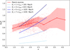 |
Fig. 1. Redshift uncertainty, δz/2, defined by the mean 1σ uncertainty, as a function of redshift for all Planck sources (red circles). The average δz/2 per redshift bin and its variance are shown as a solid red line, and the light-red filled area. The redshift interval δz/2 corresponding to comoving distances of DL = 205, 615, 1025, and 1435 Mpc h−1, between z = 1.3 and 3.0, are shown as blue lines. |
The PHz catalogue in Planck Collaboration XXXIX (2016) includes also the FIR luminosity associated with each source, derived by integrating the best-fit modified blackbody model between 8 and 1000 μm, and the SFR derived following the prescription from Kennicutt (1998). In Fig. 2 we show the total SFR and associated uncertainties as a function of redshift for the entire PHz sample. The estimated SFRs are extremely high, with the 16th and 84th percentile being 1.6 × 10⁴ M⊙ yr−1 and 3.2 × 10⁴ M⊙ yr−1 (for a dust temperature equal to 30 K). As discussed in the introduction, we resort to large volume hydrodynamical simulations to investigate the possible origins of these high SFRs.
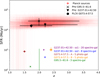 |
Fig. 2. Star formation rates as a function of redshift, and associated uncertainties, for the 2151 high-z SF Planck sources (red crosses). The Planck estimates for three sources with spectroscopically confirmed structures are highlighted with large symbols: G237.01+42.50 (upside-down black triangle), G95.5−61.6 (black cross), and G073.4−57.5 (black circle). The values derived from the spectroscopically confirmed members of these three sources are shown with coloured symbols as noted. |
2.2. PHz follow-up observations
With the aim of investigating the nature of these Planck sources, follow-up observations with the Herschel Space Observatory and with the Spitzer Space Telescope, of 228 PHz and 92 PHz sources, respectively, have been carried out (Planck Collaboration XXVII 2015; Martinache et al. 2018). In addition, optical and NIR imaging observations, and spectroscopic observations have been obtained for a handful of PHz sources. At the present time, only three PHz sources have been spectroscopically confirmed.
First, PHz G95.5−61.6 was observed by Flores-Cacho et al. (2016) from optical to sub-millimetre wavelengths, and targeted optical-NIR spectroscopic observations revealed an overdensity of sub-millimetre sources associated with two clumps of galaxies at high-redshift. They found one structure at z ∼ 1.7 with three spectroscopically confirmed galaxy members, and a second one at z ∼ 2.0 with six confirmed members. Unfortunately, the SFR of the structure at z ∼ 2.0 has not been estimated, given that two of the six galaxies are fully blended in their aperture photometry. The SFR, stellar mass, and redshift obtained from each member galaxy of the structure at z ∼ 1.7 are presented in Table 3 of Flores-Cacho et al. (2016), and will be used in this analysis.
Secondly, the Planck source PHz G073.4−57.5 has been observed with ALMA and fully investigated by Kneissl et al. (2019). They found that this sub-millimetre emitted source is composed of at least two distinct SF structures (called A and B) along the LOS: one at z ∼ 1.5 and the second one at z ∼ 2.4, and with five galaxy members for each. Beyond these two SF high-z groups, they also detected eight luminous SF galaxies along the LOS. We notice that this follow-up observation is not spectroscopic, but the photometric redshift uncertainty is about 0.15. They also provided SFRs and stellar masses for each galaxy in their Table 5. These measurements will be compared in this paper with those of the simulated protocluster members.
More recently, a third PHz source, PHz G237.01+42.50 has been thoroughly investigated by Polletta et al. (2021). This source is located in the COSMOS field and contains at least 31 spectroscopically confirmed galaxies at redshift around z ∼ 2.16. In details, this source appears to be the sum of two substructures or protocluster regions: one clump of 20 galaxy members at 2.15 < z < 2.165, and the second one with eight galaxies at 2.19 < z < 2.20. Galaxies of these two structures (called ss1 and ss2) are mostly blue SF galaxies with SFR and stellar masses consistent with the main sequence (MS), and with a significant fraction (20 ± 10%) of active galactic nuclei (AGNs). Galaxy member SFR and stellar masses used in this study are reported in Table 8 of Polletta et al. (2021).
The total SFR and stellar mass, and the redshift range of these three PHz sources containing five SF galaxy structures at high-z are reported in Table 1. In Fig. 2, we show the Planck measurements of these sources with black symbols. Their associated SFRs and redshifts, as measured from the confirmed members in the follow-up observations, are instead shown with coloured symbols. The follow-up observations indicate that some PHz sources contain at least two different structures aligned along the LOS. The follow-up observations also prove that the total SFR obtained by considering the identified SF galaxies in those structures is much lower than the SFR estimated from the Planck data.
Main properties of the structures found in the PHz sample.
3. Methods
To understand the nature of the Planck sources and reconcile their properties with those derived from the follow-up observations, we resorted to large volume cosmological simulations (see e.g. Granato et al. 2015; Bassini et al. 2020). Since not all PHz sources might contain a high-z protocluster, indeed a small percentage of them are strongly lensed galaxies (Planck Collaboration XXVII 2015; Cañameras et al. 2015, 2021), in the simulations, we questioned the Planck selection without imposing a priori that the simulated object will evolve into a massive cluster by z = 0. The fate of the simulated structures is investigated and discussed later. The issue of how to select true protoclusters in simulations has been previously discussed by Lim et al. (2021) using the TNG300 simulations. They concluded that simulated objects selected by their total SFR, rather than by halo mass, and independently of their final mass at z = 0, reproduce better protocluster observations. This is especially true for protoclusters discovered as high-SF galaxy overdensities because of their bright IR luminosity.
Starting from this point, we constructed a simulated protocluster sample, making use of the TNG300-1 simulation, selected on their total SFR. For each simulated object, we computed the total SFR from the distribution of SF galaxies within different volumes, as presented below.
3.1. TNG300-1 simulation
The IllustrisTNG project is a series of cosmological hydrodynamical simulations that simulate the formation and evolution of cosmic structures from high redshift to the present time (Nelson et al. 2019). The numerical models that govern the key physical processes relevant for galaxy formation and evolution are described in Pillepich et al. (2018). We refer to them for details on the SFR computation per gas cells in the simulations of the IllustrisTNG project. We focus here on the TNG300-1 simulation of the IllustrisTNG project (TNG300-1 hereinafter), for which the comoving size of a simulation box is about 300 Mpc, and the resolution in mass is about mDM = 4.0 × 10⁷ M⊙ h−1. TNG300-1 is the largest simulation box of the IllustrisTNG series, with the best spatial and mass resolution. This choice is optimal for probing SF structures at high redshift through their galaxy distribution. Indeed, as discussed by Lim et al. (2021), the computation of SFR can be affected by the spatial resolution of hydrodynamical simulations. The TNG300-1 simulation has 100 available snapshots, each consisting of one simulated box extracted at a specific time step from z ∼ 20 to z = 0. For each snapshot, TNG300-1 provides a halo catalogue, with halos identified by the friends-of-friends (FoF) algorithm (Davis et al. 1985), and sub-halo catalogues derived from the Subfind algorithm (Springel et al. 2001). We consider here galaxies all sub-halos with a stellar mass and an SFR larger than 0, and halos as objects detected by the FoF algorithm. Halos are constituted of both a main sub-halo (the most massive subgroup of each halo) and other sub-halos associated with it by the FoF algorithm. The simulation assumes a cosmology consistent with results from Planck Collaboration XXIV (2016), such that ΩΛ, 0 = 0.6911, Ωm, 0 = 0.3089, Ωb, 0 = 0.0486, σ8 = 0.8159, ns = 0.9667 and h = 0.6774.
3.2. Simulated most SF protocluster candidates in TNG300-1
To question the Planck selection in the simulations, we considered the most SF objects at various redshifts, even if they might not evolve into massive halos by the present time. The SFR selection was performed on the SFR of the halo, referred to later as SFRFoF. This SFR value, provided by the TNG300 simulation, is the sum of the individual SFRs of all gas cells in a FoF group. We then constructed a sample of high-z SF objects, by selecting the 30 most SF halos from z = 1.3 to z = 3 in IllustrisTNG. This redshift interval was chosen to match the redshift range covered by the Planck sources. Indeed, more than 90% of the PHz have redshifts 1.3 < z < 3. This redshift range was covered by 19 snapshots in the simulation. The choice of 30 SF halos at each redshift was based on the number of massive clusters at z = 0 in TNG300-1. Indeed, there are approximately 30 galaxy clusters with mass1M200 > 2.5 × 10¹⁴ M⊙ h−1 (similar selection as Lim et al. 2021, which have used TNG300). Therefore, our simulated sample of ‘mock protoclusters candidates’ from TNG300-1 was constituted of the 570 most SF objects at 1.3 < z < 3.
3.3. The fate of the simulated most SF objects
Starting from our simulated sample of the 570 most SF objects from z = 1.3 to z = 3, we aimed to probe their fate at z = 0. In order to test if they are actual protoclusters (e.g. progenitors of massive galaxy clusters at z = 0), we focused on their descendant at the last snapshot of the simulation (z = 0).
To derive the final mass of the descendant of each simulated object, we used the merger tree of the associated sub-halos, computed using the SubLink algorithm as provided by IllustrisTNG (see Rodriguez-Gomez et al. 2015, for details on merger tree computation). For each high-z SF halo in our simulated sample, we extracted the merger tree of its main sub-halo. Following the main principal branch of each merger tree, we could find its descendant at z = 0. To do so, we considered the last descendant at z = 0 in each merger tree. From the tree identification number, we could identify the last descendant sub-halo at z = 0, and thus the associated halo at z = 0. Through this procedure, for each halo in our high-z SF halo sample, we could derive the properties of the last descendant halo, such as the mass M200(z = 0).
Given the fact that we used a sub-halo merger tree, we could also determine whether a sub-halo will become the main sub-halo or a satellite substructure inside a given halo at z = 0. Indeed, a main sub-halo at a given redshift will not necessary remain the main sub-halo during its whole merging history. Given that halos (and sub-halos) are merging during cosmic time, a main sub-halo at high redshift can become the substructure of another halo at z = 0 (by being accreted or by a merger event). In Sect. 4, we thus investigate the fate of our 570 SF objects by considering which main halo they will be associated with at z = 0; a main sub-halo or a substructure, and its final halo mass as: a cluster mass (M200c(z = 0) > 1014 M⊙), a group mass (M200c(z = 0) = 1014 − 13 M⊙), or a low-mass object (M200c(z = 0) < 1013 M⊙).
3.4. Halo properties per volume
Given the large number of observational effects (such as aperture size and LOS contamination) in protocluster detection, and potential systematics in the measurements of their properties (such as flux limits, SED fitting and galaxy selection), it is extremely difficult to perform a fair and reliable comparison between protocluster observations and simulations. In order to estimate the total SFR of the simulated protoclusters, different methods have been considered. We can measure the total SFR in the following ways: within a sphere of physical radius R = 5 R500 (Lim et al. 2021); with a fixed radius of 10 Mpc in comoving scale (Yajima et al. 2022); with different physical radii of 1 Mpc and 100 kpc (Bassini et al. 2020); or in boxes with physical size per side of 2 Mpc (Granato et al. 2015). This large diversity of SFR protocluster estimations in simulation is the result of both different observational conditions and the highly debated theoretical predictions of the extent of high-z protoclusters (see e.g. Chiang et al. 2017; Muldrew et al. 2015).
In our case, we aimed to compare the galaxy population of our high-z simulated halo sample with three PHz sources for which follow-up observations have confirmed the presence of a structure (see Table 1). Given the different aperture size and redshift range along the LOS, from both the measurements relative to the identified members and the Planck data, we developed a parametric model which integrates the galaxy distribution inside a cylinder around each of our most SF high-z halo (see also Lovell et al. 2018, for a cylindrical parametric model to probe galaxy protoclusters). We developed this technique to be flexible in the computation of the total SFR of our simulated sample, and to be able to adapt our parametrization of the cylinder to each observed PHz and to the different methodologies adopted in measuring their integrated properties.
In practice, for each SF halo of our sample, we selected all galaxies inside a cylinder with diameter Ds and length DL, and centred on the centre of mass of the halo. This cylindrical selection of galaxy distribution took into account three basic parameters: the aperture angle, the integration along the LOS, and a minimum SFR threshold applied to the galaxies.
First, We describe the minimum galaxy SFR value SFRmin. Through this parameter, only the galaxies with an SFR above such a threshold are taken into account to reflect the minimum SFR measured in the identified members by the follow-up observations.
Secondly the angular aperture θ is the diameter of the cylinder Ds is computed as the comoving transverse distance at a given redshift z for an angular aperture of θ. The redshift evolution of such a size is illustrated in the left panel of Fig. 3, by considering different angular apertures θ = 5, 10 and 15 arcmin.
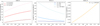 |
Fig. 3. Parameters of the cylinder parametric model, and of the simulated box as a function of redshift. Left panel: cylinder diameter Ds in comoving coordinates for three different angular sizes θ = 5, 10, and 15 arcmin. Middle panel: cylinder length as comoving distance between two redshifts z − δz/2 and z + δz/2 for three different values of δz as noted. The length of the simulation box is shown with a dotted black line. Right panel: redshift interval δz corresponding to the size of one simulation box Lbox = 205 Mpc h−1. |
Thirdly, we discuss the integration along the LOS DL. By selecting the galaxies inside a cylinder of length DL, we can artificially reproduce the integration along the LOS. This length can be converted into a redshift range δz, which is the comoving distance along the LOS between two different redshifts: z − δz/2 and z + δz/2. The middle panel of Fig. 3 shows the value of DL as a function of redshift for three different values of δz. It is important to point out that the maximum length of each cylinder is given by the comoving size of a simulation box, that is DL ≤ Lbox = 205 Mpc h−1. For each object, to compute the mean of each integrated quantity and an associated error, we considered three cylinders (with aperture θ, and length DL) centred on the halo centre and oriented in three different directions (along the x-, y-, and z-axis) that mimic three fiducial lines of sight.
The total SFR of a given halo is thus simply the sum of the SFR of all galaxies inside a cylinder with parameters θ and DL, and centred on the halo, such that:
 (1)
(1)
with Ngal the number of i galaxies with SFRi > SFRmin contained inside a cylinder defined by the θ and DL parameters, and centred on a given object at its snapshot. Similarly, the total stellar mass of a given halo is computed as:
 (2)
(2)
with M*, i being the stellar mass of i galaxies inside the same cylinder as above and centred on a given object at its snapshot. The total stellar mass and SFR of each simulated SF halos are computed in cylinders defined by the parameters θ, δz, and SFRmin, which reproduce at best the observational conditions of the PHz follow-up observations.
3.5. Mimicking the Planck measurements in the simulations
To mimic the measurements carried out with the Planck data on the full PHz sample (Planck Collaboration XXXIX 2016), we considered cylinders with aperture θ, consistent with the typical size of the PHz sources. The Planck maps used to measure the sub-millimetre flux densities of the PHz sources have a resolution of ∼5 arcmin, and the sources’ size have a major and minor axis full width half maximum of ∼10 arcmin and 5 arcmin, respectively. Thus, we chose an angular aperture θ = 10 arcmin. This angular size corresponds to cylinders with comoving diameters ranging from 8 to 12 Mpc h−1 at 1.3 < z < 3 (see Fig. 3). This size is in good agreement with the protocluster theoretical size predicted by Chiang et al. (2017), given that it is approximately twice the radial distance where membership probability drops to 50% in protoclusters at 1 < z < 3.
The length of the cylinder that should be adopted to reproduce the Planck total SFRs of the PHz sources is defined by the estimated redshift uncertainty δz described in Sect. 2. Such an uncertainty is, on average, equivalent to a comoving distance of 1025 Mpc h−1, as illustrated in Fig. 1. Such a distance is much longer than the maximum depth of a simulation box (i.e. Lbox = 205 Mpc h−1). Indeed, for each snapshot of the simulation at redshift zsnap, the maximum redshift integral δz equivalent to a comoving distance of 205 Mpc h−1, is illustrated in the right panel of Fig. 3. Thus, to take into account the contribution from the galaxies along the LOS within δz, we considered a cylinder length that combines five simulation boxes (DL = 5 Lbox = 1025 Mpc h−1), two in the foreground and two in the background of each simulated halo.
For each kth snapshot, we considered the total SFR from the most SF halo and that from the two foreground (k + 2, k + 1th) and the two background (k − 1, k − 2th) snapshots. The total SFRs from the foreground and background snapshots were obtained by averaging the total SFR given from all the galaxies within 100 random cylinders, with parameters θ = 10 arcmin, and DL = Lbox, in those snapshots. We illustrate these additional background and foreground contributions to our parametric computational method of halo SFR in Fig. 4. The total SFR of an SF halo at zk is thus derived as:
 (3)
(3)
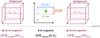 |
Fig. 4. Illustration of the SFR computation method for a given SF halo in a kth simulation snapshot at a given redshift zk. The total SFR of an object is computed by summing the SFR of the galaxies inside a cylinder of length DL(δz) and diameter Ds(θ) centred on the halo. The contributions of N background and foreground boxes along the LOS are considered by adding the mean total SFR computed inside cylinders with the same parameters DL(δz) and θ in the nearest snapshots at the lower and higher redshifts, zk − 1 and zk + 1. |
4. Results
We aim to compare our simulated sample of the 570 most SF halos from z = 1.3 to z = 3 and their associated properties, as computed by the cylinder parametric model described in Sect. 3, with both the Planck measurements of the full PHz sample, and with those obtained on three PHz sources from follow-up observations. We first investigate the total SFR of the Planck protocluster candidates by including the contribution from foreground and background sources along LOS in the simulated sample. Then, we compare the main properties (SFR, M*, and number counts) of the galaxy members identified in the spectroscopically confirmed PHz protoclusters with those in the simulations. Finally, we analyse the evolution of the most SF simulated objects up to the present time. We also investigate which physical properties in the simulated halos can be used to better predict their evolution and the final halo mass at z = 0.
4.1. Effective SFR of the Planck SF protocluster candidates
As discussed in Sect. 2, the Planck SFRs of the PHz sources were obtained by integrating the flux densities over a ∼10 arcmin region, and were expected to be highly over-estimated due to the contribution of SF galaxies along the LOS (Negrello et al. 2017). Indeed, in spite of the cleaning procedure applied to remove the contribution to the sub-millimetre flux densities from low- (z < 1) and high-(z > 4) redshift sources, the range of possible redshifts of these Planck sources remains quite large, δz ∼ 1.4 (see Fig. 1).
To compare the Planck SFR with those obtained from the simulations, we considered the most SF halos at 1.3 < z < 3 (in Sect. 3) and computed their Planck-like SFR by considering cylinders of diameter θ = 10 arcmin, and of lengths DL = 205, 615, and 1025 cMpc h−1. The total SFRs obtained from the simulations and from Planck (Planck Collaboration XXXIX 2016) are shown in Fig. 5 with red and blue symbols. The FoF SFRs of the simulated most SF halos, derived by adding the SFRs of all the bounded galaxies, are also shown as green circles. It is important to note that the Planck SFRs were divided by 1.74 to be compared with simulations, to correct from the Salpeter initial mass function (IMF; Salpeter 1955) assumed by Planck to the adopted Chabrier IMF (Chabrier 2003) in the simulations.
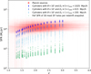 |
Fig. 5. Estimated SFRs and redshifts of the Planck high-z sources (Planck Collaboration XXXIX 2016) as measured using Planck data (red points). For comparison, the SFRs of the 30 most SF simulated halos from 19 snapshots at different redshifts are also shown. In blue, we show the simulated halos’ SFRs computed by summing the SFR of all galaxies inside cylinders with diameter θ = 10 arcmin and lengths of DL = 205, 615, and 1025 Mpc h−1 (see Sect. 3). In green are the FoF SFR values. |
The SFRs obtained by considering all simulated galaxies inside cylinders with length DL from 615 up to 1025 cMpc h−1, and aperture θ = 10 arcmin centred on the most SF simulated objects, well match the SFRs derived from the Planck photometric measurements. Conversely, these Planck-like integrated SFRs are about 25 times larger than the SFRs of most SF halos derived from the SFRs of the bounded galaxies. Thus, we argue that the SFR estimations from the Planck high-frequency maps are the result of both, at least one of which is a very luminous source, and a large contamination of foreground and background sources along the LOS projected within a region similar to the Planck beam.
It is interesting that the length of DL = 1025 cMpc h−1 corresponds approximately to the photometric Planck redshift range δz, and well matches the effective SFR of the Planck sources. Indeed, this amount of LOS contamination corresponds the associated photometric redshift range (δz ∼ 1.4; see Fig. 1) as determined by fitting a single modified blackbody to the Planck high-frequency flux densities. This similarity suggests that the uncertainty derived from the SED fitting is related to the contribution of IR sources along the LOS. We also notice that the effective SFR of the Planck sources matches with LOS contamination from 615 to 1025 cMpc h−1, whereas their redshift uncertainties are better represented by LOS distances from 1025 to 1435 cMpc h−1. This difference can be interpreted as a hint of an overestimation of the Planck redshift uncertainties.
This finding, which supposes that the effective flux (and derived SFR) of the Planck sources are overestimated due to line-of-sight effects from aligned SF galaxies integrated in a large redshift range, is consistent with both theoretical and observational studies of Planck sources. Theoretically, Negrello et al. (2017) have shown that protocluster candidates detected in the Planck maps can be interpreted as Poisson fluctuations of the number of high-z dusty protoclusters within the same Planck beam, rather then being individual clumps of physically bound galaxies. They concluded that most of the flux density within the Planck beam can be explained by one or two very luminous sources, and by a larger number of faint galaxies along the LOS. Moreover, follow-up observations also revealed that these fields often contain two SF structures aligned along the same LOS, as illustrated in Fig. 2. As discussed in Polletta et al. (2021), the total SFR from the SF galaxies, identified spectroscopically or through narrow-band imaging, in a small redshift range (z = [2.15 − 2.2]), is much smaller than the SFR derived from Planck sub-millimetre measurements, implying the need to integrate the signal along a larger redshift range in order to reproduce the Planck-derived SFR of the PHz sources. Indeed, they reproduce the Planck flux densities measured in the Planck beam of a PHz source by summing the Herschel flux densities of all the Herschel sources in the same region.
4.2. Comparison with PHz follow-up observations
Three PHz sources were followed up with dedicated observations and have yielded the discovery of significant overdensities of galaxies at similar redshifts, confirming their association with high-z protoclusters, as described in Sect. 2 and summarized in Table 1. These PHz fields, G237.01+42.50, G073.4−57.5, and G95.5−61.6, have been individually observed with distinct observational strategies (spatial and wavelength coverage, redshift measurements techniques, and depth), making direct comparisons with simulations difficult. More specifically, the overdensity in the PHz source G237.01+42.50 was found by combining spectroscopic observations at optical and near-IR wavelengths over a 10′×10′ region. These observations were biased in favour of SF galaxies with sufficiently bright emission lines at rest-frame ultraviolet or optical wavelengths to enable a spectroscopic redshift measurement (Polletta et al. 2021). Once an overdensity at a specific redshift was found, narrow-band imaging observations in a smaller region of the field were carried out to identify SF galaxies with a strong Hα line in emission at the same redshift (Koyama et al. 2021). The PHz source G073.4−57.5 has been instead observed with ALMA pointed observations targeting eight Herschel sources in a 5′×5′ region (Kneissl et al. 2019). Finally, in G95.5−61.6 optical-NIR spectroscopic observations were carried out, targeting colour-selected galaxies associated with four Herschel sources, all located in a 1′×1′ region (Flores-Cacho et al. 2016).
In this second comparison, our goal is to test whether the galaxies in and around the most SF high-z halos in IllustrisTNG can reproduce the galaxy properties observed in the overdensities found in these three PHz sources. For each overdensity, we searched for the best matched simulated halo by choosing the 30 most SF halos at the closest redshift, and for each simulated halo by selecting the galaxies using our parametric cylinder model. The parameters of the cylinder were chosen to be close to the observational configuration of each PHz observation, and are reported below.
First, two overdensities were found in PHz G237.01+42.50, both in the same 10 × 10 arcmin2 region, one containing 20 galaxies at z = 2.155 ± 0.005 (ss1) and anther with eight galaxies at z = 2.195 ± 0.005 (ss2) (Polletta et al. 2021). We therefore considered cylinders with parameters θ = 10 arcmin and δz = 0.01. In addition, since the identified members had SFRs > 10 M⊙ yr−1, only simulated galaxies with SFRs above such a value were taken into account.
Secondly, the eight ALMA pointings in PHz G073.4−57.5 covered, in total, an area of 2.4 arcmin2 and yielded mm continuum detections of 18 galaxies. Photometric or CO-based spectroscopic redshifts were derived for these galaxies, suggesting the existence of two overdensities, both with five members; one at z ∼ 1.5 and another at z ∼ 2.4 (Kneissl et al. 2019). Since the ALMA pointings and the members of each of the overdensities are distributed on a 5′×5′ region, but only 10% of it was probed by the follow-up observations, to match these overdensities, we considered cylinders with θ = 2.4 arcmin and a sufficiently large depth along the LOS to mimic the significant photo-z error (i.e. δz = 0.17 at z ∼ 1.5 and δz = 0.26 at z ∼ 2.4). We considered also an SFR threshold of 30 M⊙ yr−1, given the lowest SFR value measured in these overdensities (i.e. 44 M⊙ yr−1).
The third PHz that was spectroscopically confirmed is G95.5−61.6. This source contains two structures, one with three members at z ∼ 1.7 and a second (blended) with six members at z ∼ 2, both distributed over a 1′×1′ region (Flores-Cacho et al. 2016). Since there are no accurate SFR estimates for the structure at z ∼ 2, in the following, we considered only the structure at z ∼ 1.7. Given the tiny aperture and the precision of the spectroscopic measurements, we chose a cylinder with angular aperture θ = 1 arcmin and depth equivalent to a redshift interval of δz = 0.005. Only galaxies with SFR > 10 M⊙ yr−1 were considered.
For each of the five confirmed structures, we considered the 30 most SF halos at the snapshot redshift closest to the structure redshift. We computed their total SFR and stellar mass considering only the galaxies with SFR larger than the threshold defined above inside the appropriate cylinder. By considering three orientations (along x- y- and z-axis) for each cylinder, we artificially increased our simulated sample of 30 most SF halos to 90 SF halos in each case. The distribution of total SFRs and stellar masses for the simulated halos are compared with the measured ones in the left panels of Fig. 6. Each row refers to one of the five observed structures. We also show, on the right panels of Fig. 6, the number of galaxies inside cylinders centred on each of the 30 most SF halos as a function of total stellar mass. Black symbols refer to the observational results of the five observed structures, and coloured symbols represent the values drawn from the simulations.
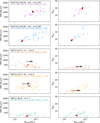 |
Fig. 6. Total SFR, and stellar masses (left panels), and number of galaxies (right panels) derived from the 30 most SF simulated objects at specific redshifts, zsnap compared with the measured values from five structures (one per row) found in three PHz sources. The selected snapshot in each row is the closest to one of the observed PHz structures. The reported quantities were obtained by averaging the total values measured in three cylinders (oriented along x, y, and z-axis) with parameters θ and δz, and considering only galaxies with SFR > SFRmin. Each row corresponds to one of the five observed structures (the name and the redshift are noted in black), and relative quantities (see Table 1) are shown with a black upside-down triangle. The snapshot redshift, the SFR threshold, and the cylinder parameters are noted in each panel in various colours, and shown as coloured circles. A red cross corresponds to the simulated halo with estimated quantities that best reproduce those of an observed structure. |
As shown in Fig. 6, our cylinder parametrization yields SFRs, stellar masses, and galaxy counts in the simulated objects that are compatible with the values measured in the five observed PHz structures. This is particularly true for G237.01+42.50-ss1 at z ∼ 2.1, G073.4−57.5-B at z ∼ 2.4, and G073.4−57.5 at z = 1.7. To better illustrate the good match between the observations and the simulations, we highlight with a red star the simulated object that is in closer agreement with the corresponding observed structure. The values of these simulated halos can be found in Table 2 for comparison with the observational ones reported in Table 1, showing the good agreement between the observed structures and the simulated SF halos. Interestingly, the most similar simulated object in the case of G237.01+42.50-ss2, is located on the tail of the SFR-stellar mass distribution of the simulated SF halos, suggesting that this structure is one of the least massive and least SF objects among the most SF halos at its redshift. The comparison with a such large sample of simulated halos shows also that the G073.4−57.5-A structure has a larger SFR than predicted by the simulations, even if the total stellar mass and the number galaxy count are well reproduced by the simulations. This discrepancy could be explained if some of the galaxy members had higher SFRs than predicted, but similar stellar masses. Since the identified members of this structure are all bright millimetre sources, they are biased in favour of galaxies with large SFRs. Such a bias was not included in the choice of the closest simulated object.
Properties of simulated halos that best reproduce the observed values.
We argue that the good agreement between simulations and observations is due to the cylinder parametric model, which allows us to take into account both the projected spatial distribution of the galaxies on the sky, and their distribution along the LOS, as derived from the observations. Taking into account only the contribution from the bound galaxies to each simulated halo would result in larger discrepancies between simulated and observed values (see e.g. the FoF SFR values in Table 2).
4.3. Galaxy properties in PHz follow-up observations
The good agreement between the total SFRs and stellar masses of the simulated objects and the observed ones, prompts us to investigate whether this is also the case for the individual galaxy members. To explore this point, we show in Fig. 7 the SFR and stellar mass of the galaxies in each observed structure (one panel per structure) as measured in the observations (black symbols), and in the simulated halo that best matches the integrated observed quantities (shown as red crosses in Fig. 6; and in coloured crosses in Fig. 7). The overall distribution of stellar mass and SFR of the galaxy members in the simulated SF halos and in the observed structures are consistent, in particular for the PHz G237.01+42.50 ss1 and ss2 structures, for which a large number of galaxy members are known. We notice that inside the G073.4−57.5 A and B structures, galaxies are apparently more massive in the A structure, and have higher SFRs in the B structure than the simulated ones. Given that the membership is based on photometric redshifts (less accurate than spectroscopic redshifts), we believe that the comparison with the cylindrical model might not be well adapted, and a proper light-cone galaxy selection might be better to interpret these observations (similar to Araya-Araya et al. 2021). Also, in G95.5−61.6, the simulated galaxies tend to be less massive and more numerous than the simulated ones, but this difference is not significant considering the small number of identified members.
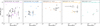 |
Fig. 7. Star formation rates as a function of stellar masses of the galaxy members in the five confirmed structures (coloured crosses) and of those drawn from the closest simulated case (black points). The simulated data were obtained from all the galaxies inside a cylinder around a specific SF halo with total SFR and stellar mass that are the closest to those measured in the observations (see red crosses in Fig. 6). Each panel shows a different structure whose name and redshift are noted in black on the top. |
We thus focus on the structure that has a large number of identified members, PHz G237.01+42.50. Since its two structures overlap in projection on the sky and are in relatively close proximity along the LOS, we consider them together for the following analysis. In Fig. 8, we show the SFR as a function of stellar mass of the 28 spectroscopic members of the two structures ss1 and ss2 (as in Fig. 16 of Polletta et al. 2021), similarly to Fig. 7. We also show the star forming MS at z = 2.17, as parametrized by Speagle et al. (2014). Although these two structures can be considered as two distinct protoclusters, their close redshifts imply that they might constitute a proto-supercluster (see Polletta et al. 2021, for a discussion on this possibility). As illustrated in Fig. 8, the observed galaxy members are consistent with the MS (assuming a Chabrier 2003 IMF). The galaxy members include both star-forming galaxies and AGN. The latter were identified through optical spectroscopy or X-ray data. The estimated AGN fraction in the two combined structures, PHz G237.01+42.50 ss1, and ss2, is 14%±10%.
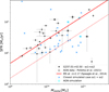 |
Fig. 8. Star formation rates as a function of stellar masses of the galaxy members in the spectroscopically confirmed structure G237+42.50 (ss1+ss2) from Polletta et al. (2021) (black stars). A grey circle indicates the AGN members. The SFR and stellar masses of the galaxies from the closest simulated case (for ss1 and ss2) are shown as blue crosses, and a cyan circle is over-plotted on those that are considered AGN. The main sequence at z = 2.17, as formulated by Speagle et al. (2014), is shown as a solid red line, and the main sequence divided by a factor of three as a dotted red line. |
For comparison, we show in Fig. 8 the galaxies in the two simulated halos that best reproduce the integrated properties of the two structures in G237.01+42.50 (see red crosses in Fig. 6) as blue crosses. In the simulations, it is possible to identify the galaxies that contain an AGN as those that host a super massive and fast accreting black hole (SMBH; with masses MBH > 108 M⊙ h−1 and instantaneous accretion rate ṀBH > 108 M⊙ h−1/(0.978 Gyr h−1)). These thresholds are such that the BHs would double their mass within roughly 1 Gyr. The thresholds represents the most luminous AGNs in massive galaxies; their bolometric luminosity is around LAGN ≳ 1044 ergs s−1, as estimated from BH model of Churazov et al. (2005; we refer to Florez et al. 2021; Habouzit et al. 2022, for details on AGN evolution and their bolometric and X-ray luminosities in TNG300). We find an AGN fraction in the simulated objects that is 11%±6% (with two AGN in the simulated object matching ss1 and one in that matching ss2). The AGN fraction in the simulated ss1 and ss2 objects is thus consistent with the observed value.
Regarding the distribution of galaxies in the SFR–M* diagram, whereas the observed galaxies are well distributed around the MS, the simulated ones have almost systematically lower SFRs. This result is consistent with the findings of Bassini et al. (2020), who find that the SFRs of high-z SF galaxies are under-predicted in the DIANOGA hydrodynamical simulation. They show that this lower normalization of the MS in simulations is stable against varying several sub-grid and AGN feedback models. This offset of the MS for high-z SF galaxies in simulation has been explored in different recent numerical studies, and the reason is still debated. A possible explanation might be linked to the underestimated gas fractions in high-z galaxies (Bassini et al. 2020), and to the spatial resolution limit in simulations (Lim et al. 2021).
4.4. The fate of protocluster candidates
As described in Sect. 3, we investigated the mass evolution of our 570 high-z most-SF halo sample up to the present time at z = 0. The results are presented in Fig. 9. We define an SF halo as progenitor of a massive cluster if its mass at the present time is M200(z = 0) > 1014 M⊙ (Chiang et al. 2017). We find that 72% of our simulated protocluster candidate sample will actually become galaxy clusters by z = 0. The rest of the simulated sample contains predominately progenitors of galaxy groups with masses between 1013 < M200 < 1014 M⊙ (26%), and a small minority (2%) will evolve into low-mass (M200 < 1013 M⊙) isolated objects at z = 0.
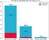 |
Fig. 9. Fractions of simulated SF halos at high-z that will evolve into clusters with halo mass M200 > 1014 M⊙, into groups with halo mass M200 = [1 − 10]×1013 M⊙, and into single halos with M200 < 1 × 10¹³ M⊙ by z = 0. We also show the fraction of simulated halos that will become the main sub-halo of a halo at z = 0 (turquoise), or a substructure (sub-halo) inside a given halo (red). |
Moreover, by considering separately the main halos and sub-halos inside a given halo at z = 0, we find that 60% of our SF simulated halo samples will become the main halo of clusters, whereas 12% of them will become other satellite substructures inside clusters. For progenitors of group-size structures at the present time, we find that only a small fraction (2%) are becoming substructures inside group-mass type objects. Finally, only 2% of the most SF halo at high-z will not merge into massive structures, but rather will stay as isolated low-mass halos at z = 0.
We note that a large number of our simulated halos will merge into the same structure by z = 0. Indeed, the 570 SF halos at 1.3 < z < 3 will yield 253 distinct halos at z = 0 (or 279 distinct sub-halos), given that they can merge or be the direct descendant from a snapshot to another at lower z. The evolutionary connection between the simulated halos drawn from different snapshots is due to our selection method. Indeed, by performing an SFR-based selection at each snapshot from z = 1.3 to z = 3, we did not distinguish if the selected halos were a direct descendant from one snapshot to the next one. Thus, by considering the progenitor at different redshifts of the same final structure we could bias our statistics on the fate of our simulated halo sample. We tested this issue in Appendix A, and find that the final percentage values are only slightly affected. The number of cluster progenitors decreases from 72% to 63%, and that of group progenitors increases from 26% to 33%. Thus, the result that the vast majority of the most SF halos at high-z will evolve into massive clusters by z = 0 remains valid.
To assess the possible range of estimated final masses of a high-z simulated halo, we show the predicted z = 0 masses of the 30 most SF halos of our simulated sample at z = 2.1 (right panel) and at 2.21 (left panel) in Fig. 10. We considered these two redshifts because they matched those of the two structures in G237.01+42.50, and we find a good agreement between the observed galaxies in the two structures and the simulated ones selected via our cylinder model (see Fig. 8). One might ask what will be the fate of the most SF simulated halo at a redshift similar to that of the G237.01+42.50 ss1 and ss2 protoclusters. In Fig. 10, we show the halo mass of the most SF halos at z = 2.1 and z = 2.21 and their final masses at z = 0. We over-plot with black points the halo masses of G237.01+42.50 ss1 and ss2, and their expected mass at the present time, as deduced from the analytical method of Steidel et al. (1998), using the galaxy overdensity, as derived by Polletta et al. (2021). The theoretically expected fate of ss1 and ss2 structures is consistent with the fate of the most SF halos at their own redshift in hydrodynamical simulations. The large scatter of halo masses from high-z to z = 0 reflects the wide spread in accretion history of structure build-up (as discussed in Rennehan et al. 2020). We estimate a 73% probability that ss1, and an 80% probability that ss2, will become massive clusters with a mass larger than 1 × 10¹⁴ M⊙ at z = 0.
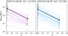 |
Fig. 10. Halo mass evolution of the 30 most SF simulated halos at z = 2.1 (purple circles connected by solid lines in the left panel) and at z = 2.21 (blue circles connected by solid lines in the right panel), showing their mass at the observed redshift and the mass of their progenitor at z = 0. The estimated halo mass of the two G237.01+42.50 ss1 and ss2 protoclusters and their expected mass at z = 0 from Polletta et al. (2021) are shown in black. |
4.5. Understanding which protocluster property best predicts its fate
Making use of the simulations, we explored whether there is an observable in protoclusters at high-z that can give hints of their fate at present times. For this analysis, we considered the intrinsic halo properties at the observed zhalo, as defined by the FoF catalogue, such as the halo mass M200, the redshift, the FoF SFR, and the number of galaxy members (defined as the hosted sub-halos within each FoF halo; Nelson et al. 2019). For each halo, we also defined an SFR fraction as:
 (4)
(4)
where Ngal is the number of galaxies gravitationally bound to a given halo based on the FoF algorithm. For each i galaxy associated with a given FoF halo, we noted its star formation rate SFRi. The SFR fraction fSFR thus defines the contribution of the most SF galaxy to the total SFR of its parent halo.
We also quantified the number of galaxies per halo using an SFR threshold to remove low-SF galaxies that would be challenging to spectroscopically identify as protocluster members in moderately deep observations. We chose an SFR threshold SFRgal = 10 M⊙ yr−1, as done to reproduce the observations discussed in this work.
The results are presented in Fig. 11, where we show the halo mass at their redshift, zhalo as a function of their total SFR for the full sample of 570 simulated halos. In each panel, we colour-code the symbols according to a specific property, the final halo mass at z = 0 (top left panel), the redshift (top right panel), the number of SF galaxies with SFR > 10 M⊙ yr−1 (bottom right panel), and the SFR fraction fSFR (bottom right panel).
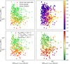 |
Fig. 11. Distribution of mass M200c and SFR of our sample of 570 simulated high-z SF halos, coloured by their fate at z = 0 (top left panel), their redshift (top right panel), their number of SF galaxy members with galaxies are SFR > 10 M⊙ yr−1 (bottom left panel), and their SFR fraction (as defined in Eq. (4), bottom right panel). |
As we can see in the top left panel, the fate at z = 0 of our SF halo sample is strongly governed by the halo mass at z = zhalo. As expected, a massive halo at high-z is supposed to grow by accretion and merger to become a more massive structure at z = 0, following hierarchical formation scenario. Interestingly, the total SFR of a high-z halo is not a good parameter to establish whether it will evolve into a massive cluster at z = 0. Indeed, the final mass of a high-z halo depends mainly on its mass at its redshift, and not on its total SFR.
One might question whether this is the result of our halo selection where we considered only the most SF halos from z = 1.3 to z = 3. In the top right panel, we probe the dependence of the halo properties on their redshift. We can see that the redshift of the simulated SF halos does not have an impact on their fate. On the other hand, there is a relation between the halo redshift and the halo SFR, with halos at higher redshifts being more SF than those at lower z. As illustrated in Fig. 5, and also shown over a wide (from z = 0 up to z = 7) redshift range in Lim et al. (2021), the SFRs of cluster progenitors are supposed to peak at around z ∼ 3 − 4, and decrease from z ∼ 3 to z = 0.
We now examine whether the fate of the high-z SF halos can be predicted based on their galaxy properties at the observed redshift (bottom panels of Fig. 11). For this analysis, we consider the number of galaxies above a minimum SFR of 10 M⊙ yr−1 within each high-z halo (Ngal; bottom left panel), and the SFR fraction (fSFR; bottom right panel). The smaller the number of galaxy members or the higher the SFR fraction (meaning that the total SFR is dominated by a single galaxy), the more a high-z SF halo leans towards an isolated low-mass structure at z = 0. Conversely, high-z halos with a more even distribution of SFRs over a relatively large number of SF galaxies (rather than having a single dominant galaxy with a very high SFR) are more likely to evolve into massive clusters at the present time.
To investigate the relation between the global halo properties and those of the galaxy members, we analyse the halo mass – SFR distribution of the high-z SF halos in three bins of the number of SF galaxy members (Ngal below 3, between 3 and 10, and larger than 10; see different coloured symbols in the bottom left panel of Fig. 11). This binning in SF galaxy number well reproduces the distribution in final mass of the high-z halos (as shown by comparing the top and bottom left panels). The number of SF galaxies in a high-z halo is, indeed, a strong indicator of its fate at z = 0. Interestingly, this relation is independent of the total SFR of the halo, although we have to keep in mind that our sample might not probe a sufficiently broad range of total SFRs to show significant trends with it as it contains only the most SF halos at each redshift snapshot. In summary, the more populated an SF halo is, independently of its redshift (from z = 1.3 to 3), the higher the chance it will become a massive cluster by z = 0. More quantitatively, having more than seven SF galaxies gravitationally bound appears to be a strong hint that it is actually a massive cluster-progenitor. Indeed, the probability that a high-z SF halo with more than seven SF galaxies in our sample is a massive cluster progenitor is about 92%.
Such a result provides a powerful diagnostic for interpreting SF protocluster candidates at high redshift (1 ≲ z < 3). This is consistent with some theoretical models (see e.g. Steidel et al. 1998), and argues in favour of using overdensities of SF galaxies to trace the most-massive dark matter structures at high-z (Cowley et al. 2016). Furthermore, this is in line with Planck (Planck Collaboration XVIII 2014) exhibiting a correlation between dark matter halos and the CIB (Puget et al. 1996; Hauser & Dwek 2001; Dole et al. 2006), in stacks, highlighting the relationship between dark matter halos and star formation. In general, the detection of a protocluster candidate is more reliable if it is supported by a high value of galaxy overdensity (galaxy density in a source in contrast to the galaxy density field). Our analysis suggests that, rather than an extreme value of SFR from an individual high-z galaxy, a large overdensity of SF galaxies is a more powerful indicator for finding massive cluster progenitors at z = 0.
5. Discussion
With a new approach, using state-of-the-art hydrodynamics simulations, we investigated the type of high-z structures that are selected as bright and red sub-millimetre sources in the Planck maps, the so called PHz sources (Planck Collaboration XXXIX 2016; Planck Collaboration XXIV 2016). We find that the high observed Planck sub-millimetre flux densities, and thus SFRs, are reproduced by the simulations if multiple structures at 1.3 < z < 3 along the LOS are taken into account. However, most of the PHz sources seem to contain a high-z star-forming structure that will evolve into a massive cluster by z = 0, confirming their protocluster nature. These results are consistent with previous findings, both from theoretical works (Negrello et al. 2017), and from observations (Flores-Cacho et al. 2016; Kneissl et al. 2019; Koyama et al. 2021; Polletta et al. 2021, 2022).
Notably, we established a new diagnostic to assess whether a high-z (z > 1.3) structure is a star-forming protocluster that will become a massive cluster by z = 0. This can be gauged by combining the following observables: (a) the number of star-forming galaxies in the structure (i.e. N > 7), and (b) the distribution of star formation among all galaxy members (i.e. better to have a more even distribution than a single highly star forming member; see Figs. 9 and 11). This diagnostic is easy to apply and extremely useful in order to select the most promising structures for further studies and for additional follow-up observations.
Comparisons between observed protoclusters and numerical predictions have been already attempted in the past, but they remain extremely difficult given both observational and simulation aspects. Firstly, the observational selection and measurements are hardly reproducible in simulations, as these would require precise mock observations from light-cone construction (to accurately account for LOS contributions), knowledge of the galaxy spatial and redshift distributions, and mock images would need to be created with all observational effects (e.g. noise, depth, PSF, angular and sampling effects, among others). Secondly, the capacity of hydrodynamical simulations to accurately reproduce high-SF galaxies at high-z is still controversial. This could be due to the limited resolution of the simulations (Lim et al. 2021), the biases introduced by the SED fitting models (Nelson et al. 2021), the adopted dust model in the simulations, and far-field blending effects (Lovell et al. 2021).
Our cylindrical model is the first attempt to explain the Planck high-z SF protocluster candidate sample by using SF galaxy distributions from hydrodynamical simulations (and not just mass-selected samples in simulations). Currently, there is no common established technique to estimate the SFR of galaxy protoclusters in simulations (some considering integrated aperture depending on the halo radius R500, or other using a fixed aperture in comoving or physical scales). We thus developed a simple parametric model that integrated galaxies inside a cylinder centred on the area of interest (i.e. the most SF halos). We argue that such a method provides a good agreement with Planck follow-up observations, and fairly reproduces the PHz protocluster measurements. However, it is important to emphasize that a proper reproduction of the Planck selection would require the use of light-cone simulations, even if the number of protoclusters found in a specific redshift range is limited by the light-cone volume. Therefore, light-cones might provide a better solution to specifically assess the completeness and purity of cluster and protocluster detections by creating mock data images, and might thus be constructed over N-body simulations (Blaizot et al. 2005; Ascaso et al. 2016; Krefting et al. 2020; Araya-Araya et al. 2021). Exploring the complete projection of SF source distribution from z = 1.3 and 3 in hydrodynamical simulation and inside Planck beam size will be the next necessary step to accurately evaluate the number of sources and their individual contributions along the large LOS integration (as δz ∼ 1.4).
6. Conclusions
The main goal of this work was to investigate the nature of the Planck selected high-z sources and the origin of their bright sub-millimetre flux densities, and high SFRs. To this end, we examined the spatial distribution and the properties of the SF galaxies associated with these bright Planck sources using state-of-the-art hydrodynamical simulations. The PHz were detected in the Planck high-frequency maps (over the cleanest 26% of the sky), after removing Galactic dust emission (and sub-millimetre emission from sources at z < 1), and CMB contamination (and emission from z > 4 sources). The more than 2100 PHz sources with estimated redshifts around z ∼ 2, represent an ideal sample for investigating the most active sites of star formation during the epoch of peak activity (i.e. from z ∼ 1 to 3), the so-called cosmic noon (Madau & Dickinson 2014; Chiang et al. 2017).
In this work, we selected a sample of 570 high-z SF objects representing the thirty most SF halos at 19 different redshifts from z = 1.3 to z = 3 in the TNG300 simulation of the IllustrisTNG project (Nelson et al. 2019). This SFR-based selection technique provides a better representation of the observed protoclusters than other selections based for example on mass, as also shown by Lim et al. (2021). The properties of these simulated objects were computed by considering the galaxy distribution inside parametric cylinders centred on each SF halo, in order to reproduce the aperture window size of the observations, and possible LOS contaminations (integral in redshift range), an effect discussed by Negrello et al. (2017). This cylindrical toy model was designed to select the galaxies associated with each high-z SF object in the simulations, to compute their total SFR, and stellar mass, and to characterize their galaxy member properties. We compare the properties of the simulated high-z SF objects with the Planck measurements derived for the whole PHz sample and with more detailed observations carried out for three PHz sources, for which significant galaxy overdensities have been found through spectroscopic observations (Flores-Cacho et al. 2016; Kneissl et al. 2019; Polletta et al. 2021). The results of this comparison are summarized below:
-
(1)
The total SFR of the PHz sources, measured from the Planck flux densities, can be reproduced in the simulations by taking into account the contribution of the most SF halos at specific redshifts, and the contribution of the galaxies along the LOS distributed over a redshift interval consistent with a distance of 1025 comoving Mpc h−1. This result implies a large contamination in the Planck sub-millimetre measurements from background and foreground galaxies along the LOS. This LOS contamination is in agreement with Negrello et al. (2017) who find, from a semi-analytical analysis, that the high-SF sources detected in the Planck maps can be interpreted as the sum of at least one high-SF halo, and of a strong contamination from high-z dusty galaxies along the LOS, both contributing within the Planck beam. This finding is also consistent with results obtained from follow-up observations of Planck sources. The observations indeed reveal at least two distinct SF structures aligned along the LOS, and that the SFR derived from the Planck data cannot be explained by the galaxies in one high-z structure (suggesting the need for a significant contribution from galaxies along the LOS but projected within the Planck beam).
-
(2)
The number of galaxy members and the total stellar mass and SFR of the spectroscopically confirmed structures found in three PHz sources through dedicated follow-up observations (Polletta et al. 2021; Kneissl et al. 2019; Flores-Cacho et al. 2016) are reproduced by the simulations. This good agreement is obtained by considering the most SF simulated halos at a redshift close to the observed one, and the SF galaxy population with an SFR above a certain limit and distributed within a cylinder of diameter and length consistent with the volume occupied by the confirmed members. Our cylinder parametric model can thus reproduce the PHz confirmed structures with high-z SF simulated objects in terms of the number of galaxy members, total stellar mass, and total SFR.
-
(3)
In more detail, comparing the values of SFR and stellar mass of the individual galaxy members in the observed structures and in the simulated SF objects gives a good agreement. In one case (i.e. in G237.01+42.50), we were also able to test whether the fraction of AGN in the observed structure was consistent with that found in the simulation, finding a good agreement. The distribution of simulated galaxies with respect to the MS at their redshift was, however, shifted to lower values in SFR compared to that of the observed galaxies. This discrepancy is consistent with the results reported by Bassini et al. (2020) where the normalization of the MS at z ∼ 2.15 is under-predicted by a factor of about two to three. This implies that, even if the total mass and SFR appear coherent with the data by integrating the galaxy distribution in a cylinder, the intrinsic under-prediction problem of galaxy SFRs in simulation at high-z is not fully solved (Granato et al. 2015; Lim et al. 2021).
-
(4)
Following these three last findings, we can conclude that our sample of the most SF simulated halos at high-z is representative of the Planck sources when considering both the Planck measurements and the spectroscopic observations. We can thus predict their fate at z = 0 by probing the evolution of the simulated halo sample. We find that between 63% and 72% of our sample will actually become massive galaxy clusters with M200 > 1014 M⊙ by z = 0. It is important to point out that a significant, although minor, portion of them will evolve into a substructure inside a massive group or cluster (∼15%).
-
(5)
One might ask which physical properties of these high-z SF halos can give a hint about their fate at z = 0. We find that, rather than the high value of SFR per galaxy, the number of SF galaxy members inside a halo (typically larger than SFR > 10 M⊙ yr−1) is an indicator of their evolution at z = 0. In more details, high-z halos which are populated by more than seven SF galaxies have a higher probability of being actual cluster progenitors. This finding argues in favour of using overdensities of SF galaxies to trace the most massive dark matter structures at high-z (Cowley et al. 2016) and could be a new diagnostic to select high-z protoclusters.
-
(6)
By comparing simulations and observations based on an SFR selection, we confirm that the original Planck selection of PHz, despite LOS contamination, efficiently selects high-z (z ∼ 2) SF galaxy protoclusters, progenitors of z = 0 massive clusters, or substructures of clusters.
As discussed in Sect. 5, this analysis was a first step towards explaining the Planck sources by considering the properties of the SF galaxy population in hydrodynamical simulations. To achieve a fairer comparison with the Planck protocluster candidate selection and reproduce with fidelity the flux limit selection, it would be necessary to perform a light-cone analysis and create mock galaxy SEDs (similarly to Araya-Araya et al. 2021). Indeed a close agreement between our simulations and the observed SFR distribution from Planck is not expected because we do not exactly reproduce either the selection criteria or the SFR measurement procedure as adopted in Planck Collaboration XXXIX (2016). In conclusion, we confirm, from hydrodynamical simulation, the analytical finding from Negrello et al. (2017) about the interpretation of extremely high sub-millimetre flux from Planck sources as positive Poisson fluctuations of the number of high-z dusty protoclusters within the same Planck beam. The comparison with the spectroscopically confirmed structures argues in favour of a good agreement between observed SFRs and simulations using a parametric cylinder integral around the high-z SF halos, but it also demonstrates that high-z simulated galaxies suffer from SFR deficit. This result illustrates the long standing difficulty for numerical simulations to reproduce accurately the SFR of galaxies at the peak of the cosmic SFR density, the cosmic noon (Granato et al. 2015; Davé et al. 2016, 2019; McCarthy et al. 2017; Donnari et al. 2019; Bassini et al. 2020; Lim et al. 2021; Yajima et al. 2022).
M200 is defined as the total mass of a group enclosed in a sphere whose mean density is 200 times the critical density of the Universe, at the time the halo is considered.
Acknowledgments
The authors thank an anonymous referee for their useful comments and suggestions. This research has been supported by the funding for the ByoPiC project from the European Research Council (ERC) under the European Union’s Horizon 2020 research and innovation program grant agreement ERC-2015-AdG 695561 (ByoPiC, https://byopic.eu). The authors thank the very useful comments and discussions with all the members of the ByoPiC team. We thank the IllustrisTNG collaboration for providing free access to the data used in this work. C.G. is supported by a KIAS Individual Grant (PG085001) at Korea Institute for Advanced Study.
References
- An, F., Vaccari, M., Smail, I., et al. 2021, MNRAS, 507, 2643 [NASA ADS] [CrossRef] [Google Scholar]
- Araya-Araya, P., Vicentin, M. C., Sodré, L., Jr., Overzier, R. A., & Cuevas, H. 2021, MNRAS, 504, 5054 [NASA ADS] [CrossRef] [Google Scholar]
- Ascaso, B., Benítez, N., Dupke, R., et al. 2016, MNRAS, 456, 4291 [NASA ADS] [CrossRef] [Google Scholar]
- Ata, M., Kitaura, F.-S., Lee, K.-G., et al. 2021, MNRAS, 500, 3194 [Google Scholar]
- Bassini, L., Rasia, E., Borgani, S., et al. 2020, A&A, 642, A37 [NASA ADS] [CrossRef] [EDP Sciences] [Google Scholar]
- Beelen, A., Omont, A., Bavouzet, N., et al. 2008, A&A, 485, 645 [NASA ADS] [CrossRef] [EDP Sciences] [Google Scholar]
- Blaizot, J., Wadadekar, Y., Guiderdoni, B., et al. 2005, MNRAS, 360, 159 [NASA ADS] [CrossRef] [Google Scholar]
- Bleem, L. E., Stalder, B., de Haan, T., et al. 2015, ApJS, 216, 27 [Google Scholar]
- Böhringer, H., Schuecker, P., Guzzo, L., et al. 2004, A&A, 425, 367 [NASA ADS] [CrossRef] [EDP Sciences] [Google Scholar]
- Cañameras, R., Nesvadba, N. P. H., Guery, D., et al. 2015, A&A, 581, A105 [Google Scholar]
- Cañameras, R., Nesvadba, N. P. H., Kneissl, R., et al. 2021, A&A, 645, A45 [EDP Sciences] [Google Scholar]
- Casey, C. M. 2016, ApJ, 824, 36 [CrossRef] [Google Scholar]
- Chabrier, G. 2003, PASP, 115, 763 [Google Scholar]
- Cheng, T., Clements, D. L., Greenslade, J., et al. 2019, MNRAS, 490, 3840 [NASA ADS] [CrossRef] [Google Scholar]
- Chiang, Y.-K., Overzier, R., & Gebhardt, K. 2014, ApJ, 782, L3 [NASA ADS] [CrossRef] [Google Scholar]
- Chiang, Y.-K., Overzier, R. A., Gebhardt, K., & Henriques, B. 2017, ApJ, 844, L23 [Google Scholar]
- Churazov, E., Sazonov, S., Sunyaev, R., et al. 2005, MNRAS, 363, L91 [NASA ADS] [Google Scholar]
- Clements, D. L., Braglia, F. G., Hyde, A. K., et al. 2014, MNRAS, 439, 1193 [NASA ADS] [CrossRef] [Google Scholar]
- Cohn, J. D., & White, M. 2008, MNRAS, 385, 2025 [NASA ADS] [CrossRef] [Google Scholar]
- Cowley, W. I., Lacey, C. G., Baugh, C. M., & Cole, S. 2016, MNRAS, 461, 1621 [NASA ADS] [CrossRef] [Google Scholar]
- Daddi, E., Valentino, F., Rich, R. M., et al. 2021, A&A, 649, A78 [NASA ADS] [CrossRef] [EDP Sciences] [Google Scholar]
- Dannerbauer, H., Kurk, J. D., De Breuck, C., et al. 2014, A&A, 570, A55 [NASA ADS] [CrossRef] [EDP Sciences] [Google Scholar]
- Davé, R., Thompson, R., & Hopkins, P. F. 2016, MNRAS, 462, 3265 [Google Scholar]
- Davé, R., Anglés-Alcázar, D., Narayanan, D., et al. 2019, MNRAS, 486, 2827 [Google Scholar]
- Davis, M., Efstathiou, G., Frenk, C. S., & White, S. D. M. 1985, ApJ, 292, 371 [Google Scholar]
- Dole, H., Lagache, G., Puget, J. L., et al. 2006, A&A, 451, 417 [NASA ADS] [CrossRef] [EDP Sciences] [Google Scholar]
- Donnari, M., Pillepich, A., Nelson, D., et al. 2019, MNRAS, 489, 3036 [NASA ADS] [CrossRef] [Google Scholar]
- Dowell, C. D., Conley, A., Glenn, J., et al. 2014, ApJ, 780, 75 [Google Scholar]
- Flores-Cacho, I., Pierini, D., Soucail, G., et al. 2016, A&A, 585, A54 [NASA ADS] [CrossRef] [EDP Sciences] [Google Scholar]
- Florez, J., Jogee, S., Guo, Y., et al. 2021, MNRAS, 508, 762 [NASA ADS] [CrossRef] [Google Scholar]
- Granato, G. L., Ragone-Figueroa, C., Domínguez-Tenreiro, R., et al. 2015, MNRAS, 450, 1320 [NASA ADS] [CrossRef] [Google Scholar]
- Greenslade, J., Clements, D. L., Cheng, T., et al. 2018, MNRAS, 476, 3336 [NASA ADS] [CrossRef] [Google Scholar]
- Habouzit, M., Somerville, R. S., Li, Y., et al. 2022, MNRAS, 509, 3015 [Google Scholar]
- Hauser, M. G., & Dwek, E. 2001, ARA&A, 39, 249 [Google Scholar]
- Hill, R., Chapman, S., Scott, D., et al. 2020, MNRAS, 495, 3124 [NASA ADS] [CrossRef] [Google Scholar]
- Ivison, R. J., Swinbank, A. M., Smail, I., et al. 2013, ApJ, 772, 137 [NASA ADS] [CrossRef] [Google Scholar]
- Kalita, B. S., Daddi, E., Coogan, R. T., et al. 2021, MNRAS, 503, 1174 [NASA ADS] [CrossRef] [Google Scholar]
- Kauffmann, G., White, S. D. M., Heckman, T. M., et al. 2004, MNRAS, 353, 713 [Google Scholar]
- Kennicutt, R. C., Jr. 1998, ARA&A, 36, 189 [Google Scholar]
- Kneissl, R., Polletta, M. D. C., Martinache, C., et al. 2019, A&A, 625, A96 [NASA ADS] [CrossRef] [EDP Sciences] [Google Scholar]
- Koyama, Y., Polletta, M. D. C., Tanaka, I., et al. 2021, MNRAS, 503, L1 [NASA ADS] [CrossRef] [Google Scholar]
- Krefting, N., Sajina, A., Lacy, M., et al. 2020, ApJ, 889, 185 [NASA ADS] [CrossRef] [Google Scholar]
- Lagache, G., Puget, J.-L., & Dole, H. 2005, ARA&A, 43, 727 [NASA ADS] [CrossRef] [Google Scholar]
- Lammers, C., Hill, R., Lim, S., et al. 2022, MNRAS, 514, 5004 [NASA ADS] [CrossRef] [Google Scholar]
- Lim, S., Scott, D., Babul, A., et al. 2021, MNRAS, 501, 1803 [Google Scholar]
- Lovell, C. C., Thomas, P. A., & Wilkins, S. M. 2018, MNRAS, 474, 4612 [NASA ADS] [CrossRef] [Google Scholar]
- Lovell, C. C., Geach, J. E., Davé, R., Narayanan, D., & Li, Q. 2021, MNRAS, 502, 772 [NASA ADS] [CrossRef] [Google Scholar]
- Madau, P., & Dickinson, M. 2014, ARA&A, 52, 415 [Google Scholar]
- Magnelli, B., Lutz, D., Saintonge, A., et al. 2014, A&A, 561, A86 [NASA ADS] [CrossRef] [EDP Sciences] [Google Scholar]
- Martinache, C., Rettura, A., Dole, H., et al. 2018, A&A, 620, A198 [NASA ADS] [CrossRef] [EDP Sciences] [Google Scholar]
- McCarthy, I. G., Schaye, J., Bird, S., & Le Brun, A. M. C. 2017, MNRAS, 465, 2936 [Google Scholar]
- McConachie, I., Wilson, G., Forrest, B., et al. 2022, ApJ, 926, 37 [NASA ADS] [CrossRef] [Google Scholar]
- Muldrew, S. I., Hatch, N. A., & Cooke, E. A. 2015, MNRAS, 452, 2528 [NASA ADS] [CrossRef] [Google Scholar]
- Negrello, M., González-Nuevo, J., Magliocchetti, M., et al. 2005, MNRAS, 358, 869 [CrossRef] [Google Scholar]
- Negrello, M., Gonzalez-Nuevo, J., De Zotti, G., et al. 2017, MNRAS, 470, 2253 [NASA ADS] [CrossRef] [Google Scholar]
- Nelson, D., Springel, V., Pillepich, A., et al. 2019, Comput. Astrophys. Cosmol., 6, 2 [Google Scholar]
- Nelson, E. J., Tacchella, S., Diemer, B., et al. 2021, MNRAS, 508, 219 [NASA ADS] [CrossRef] [Google Scholar]
- Oteo, I., Ivison, R. J., Dunne, L., et al. 2018, ApJ, 856, 72 [Google Scholar]
- Overzier, R. A. 2016, A&ARv, 24, 14 [Google Scholar]
- Pillepich, A., Springel, V., Nelson, D., et al. 2018, MNRAS, 473, 4077 [Google Scholar]
- Planck Collaboration XVIII. 2014, A&A, 571, A18 [NASA ADS] [CrossRef] [EDP Sciences] [Google Scholar]
- Planck Collaboration XXIX. 2014, A&A, 571, A29 [NASA ADS] [CrossRef] [EDP Sciences] [Google Scholar]
- Planck Collaboration XXVII. 2015, A&A, 582, A30 [NASA ADS] [CrossRef] [EDP Sciences] [Google Scholar]
- Planck Collaboration XXIV. 2016, A&A, 594, A24 [NASA ADS] [CrossRef] [EDP Sciences] [Google Scholar]
- Planck Collaboration XXXIX. 2016, A&A, 596, A100 [NASA ADS] [CrossRef] [EDP Sciences] [Google Scholar]
- Polletta, M., Soucail, G., Dole, H., et al. 2021, A&A, 654, A121 [NASA ADS] [CrossRef] [EDP Sciences] [Google Scholar]
- Polletta, M., Dole, H., Martinache, C., et al. 2022, A&A, 662, A85 [NASA ADS] [CrossRef] [EDP Sciences] [Google Scholar]
- Puget, J. L., Abergel, A., Bernard, J. P., et al. 1996, A&A, 308, L5 [Google Scholar]
- Rennehan, D., Babul, A., Hayward, C. C., et al. 2020, MNRAS, 493, 4607 [NASA ADS] [CrossRef] [Google Scholar]
- Rodriguez-Gomez, V., Genel, S., Vogelsberger, M., et al. 2015, MNRAS, 449, 49 [Google Scholar]
- Rosati, P., Della Ceca, R., Norman, C., & Giacconi, R. 1998, ApJ, 492, L21 [NASA ADS] [CrossRef] [Google Scholar]
- Rosati, P., Borgani, S., & Norman, C. 2002, ARA&A, 40, 539 [Google Scholar]
- Rotermund, K. M., Chapman, S. C., Phadke, K. A., et al. 2021, MNRAS, 502, 1797 [NASA ADS] [CrossRef] [Google Scholar]
- Rykoff, E. S., Rozo, E., Hollowood, D., et al. 2016, ApJS, 224, 1 [NASA ADS] [CrossRef] [Google Scholar]
- Salpeter, E. E. 1955, ApJ, 121, 161 [Google Scholar]
- Sheth, R. K., & Tormen, G. 1999, MNRAS, 308, 119 [Google Scholar]
- Shi, D. D., Cai, Z., Fan, X., et al. 2021, ApJ, 915, 32 [NASA ADS] [CrossRef] [Google Scholar]
- Smail, I., Geach, J. E., Swinbank, A. M., et al. 2014, ApJ, 782, 19 [NASA ADS] [CrossRef] [Google Scholar]
- Speagle, J. S., Steinhardt, C. L., Capak, P. L., & Silverman, J. D. 2014, ApJS, 214, 15 [Google Scholar]
- Springel, V., White, S. D. M., Tormen, G., & Kauffmann, G. 2001, MNRAS, 328, 726 [Google Scholar]
- Steidel, C. C., Adelberger, K. L., Dickinson, M., et al. 1998, ApJ, 492, 428 [Google Scholar]
- Umehata, H., Tamura, Y., Kohno, K., et al. 2014, MNRAS, 440, 3462 [Google Scholar]
- Umehata, H., Tamura, Y., Kohno, K., et al. 2015, ApJ, 815, L8 [Google Scholar]
- Vieira, J. D., Crawford, T. M., Switzer, E. R., et al. 2010, ApJ, 719, 763 [NASA ADS] [CrossRef] [Google Scholar]
- Yajima, H., Abe, M., Khochfar, S., et al. 2022, MNRAS, 509, 4037 [Google Scholar]
- Zheng, X. Z., Cai, Z., An, F. X., Fan, X., & Shi, D. D. 2021, MNRAS, 500, 4354 [Google Scholar]
Appendix A: Testing the main progenitor problem on the statistics of the fate of SF high-z halos
Given that we performed an SFR-based selection of halos at each snapshot from z = 1.3 to 3, we might in principle consider the same SF halo at a different time step. It is thus legitimate to wonder whether these ‘replicated’ simulated halos significantly affect our statistics on their fate at z = 0. To address this issue, we re-performed the analysis described in Sect. 4.4, but after removing all objects that are direct progenitors of the same z = 0 structure, leaving only the main progenitor the first time (at the highest z) it appears. To find these direct progenitors, we considered the objects which belong to the main progenitor branch of the same merger tree (the main progenitor of each sub-halo is defined as the one with the ‘most massive history’ behind it). For example, in almost each of the 19 snapshots from z = 1.3 to 3, we had in our sample the main progenitor of the most massive cluster at z = 0 (17 times). Through this technique, we find that 173 objects, in our sample of 570 SF halos, are the direct main progenitors of 33 structures at z = 0. After removing the replicated halos, the ‘cleaned’ halo sample contains 430 distinct high-z SF halos. As shown in Fig. A.1, removing the replicated halos from our same does not change drastically the results. The fraction of SF halos at high-z that will become galaxy massive clusters at z = 0 decreases from 72% to 63%. As expected, most of the replicated halos are the most massive ones at the observed redshift, which often coincide with the progenitors of the most massive structures at z = 0.
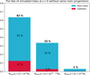 |
Fig. A.1. Fractions of 430 distinct (not evolutionary connected) simulated SF halos at high-z that will evolve into clusters with halo mass M200 > 1014 M⊙, into groups with halo mass M200 = [1 − 10]×1013 M⊙, and into single halos with M200 < 1 × 10¹³ M⊙. We also show the fraction of simulated halos that will become the main sub-halo of a halo at z = 0 (turquoise), or a substructure (sub-halo) inside a given halo (red). |
All Tables
All Figures
|
Fig. 1. Redshift uncertainty, δz/2, defined by the mean 1σ uncertainty, as a function of redshift for all Planck sources (red circles). The average δz/2 per redshift bin and its variance are shown as a solid red line, and the light-red filled area. The redshift interval δz/2 corresponding to comoving distances of DL = 205, 615, 1025, and 1435 Mpc h−1, between z = 1.3 and 3.0, are shown as blue lines. |
| In the text | |
|
Fig. 2. Star formation rates as a function of redshift, and associated uncertainties, for the 2151 high-z SF Planck sources (red crosses). The Planck estimates for three sources with spectroscopically confirmed structures are highlighted with large symbols: G237.01+42.50 (upside-down black triangle), G95.5−61.6 (black cross), and G073.4−57.5 (black circle). The values derived from the spectroscopically confirmed members of these three sources are shown with coloured symbols as noted. |
| In the text | |
|
Fig. 3. Parameters of the cylinder parametric model, and of the simulated box as a function of redshift. Left panel: cylinder diameter Ds in comoving coordinates for three different angular sizes θ = 5, 10, and 15 arcmin. Middle panel: cylinder length as comoving distance between two redshifts z − δz/2 and z + δz/2 for three different values of δz as noted. The length of the simulation box is shown with a dotted black line. Right panel: redshift interval δz corresponding to the size of one simulation box Lbox = 205 Mpc h−1. |
| In the text | |
|
Fig. 4. Illustration of the SFR computation method for a given SF halo in a kth simulation snapshot at a given redshift zk. The total SFR of an object is computed by summing the SFR of the galaxies inside a cylinder of length DL(δz) and diameter Ds(θ) centred on the halo. The contributions of N background and foreground boxes along the LOS are considered by adding the mean total SFR computed inside cylinders with the same parameters DL(δz) and θ in the nearest snapshots at the lower and higher redshifts, zk − 1 and zk + 1. |
| In the text | |
|
Fig. 5. Estimated SFRs and redshifts of the Planck high-z sources (Planck Collaboration XXXIX 2016) as measured using Planck data (red points). For comparison, the SFRs of the 30 most SF simulated halos from 19 snapshots at different redshifts are also shown. In blue, we show the simulated halos’ SFRs computed by summing the SFR of all galaxies inside cylinders with diameter θ = 10 arcmin and lengths of DL = 205, 615, and 1025 Mpc h−1 (see Sect. 3). In green are the FoF SFR values. |
| In the text | |
|
Fig. 6. Total SFR, and stellar masses (left panels), and number of galaxies (right panels) derived from the 30 most SF simulated objects at specific redshifts, zsnap compared with the measured values from five structures (one per row) found in three PHz sources. The selected snapshot in each row is the closest to one of the observed PHz structures. The reported quantities were obtained by averaging the total values measured in three cylinders (oriented along x, y, and z-axis) with parameters θ and δz, and considering only galaxies with SFR > SFRmin. Each row corresponds to one of the five observed structures (the name and the redshift are noted in black), and relative quantities (see Table 1) are shown with a black upside-down triangle. The snapshot redshift, the SFR threshold, and the cylinder parameters are noted in each panel in various colours, and shown as coloured circles. A red cross corresponds to the simulated halo with estimated quantities that best reproduce those of an observed structure. |
| In the text | |
|
Fig. 7. Star formation rates as a function of stellar masses of the galaxy members in the five confirmed structures (coloured crosses) and of those drawn from the closest simulated case (black points). The simulated data were obtained from all the galaxies inside a cylinder around a specific SF halo with total SFR and stellar mass that are the closest to those measured in the observations (see red crosses in Fig. 6). Each panel shows a different structure whose name and redshift are noted in black on the top. |
| In the text | |
|
Fig. 8. Star formation rates as a function of stellar masses of the galaxy members in the spectroscopically confirmed structure G237+42.50 (ss1+ss2) from Polletta et al. (2021) (black stars). A grey circle indicates the AGN members. The SFR and stellar masses of the galaxies from the closest simulated case (for ss1 and ss2) are shown as blue crosses, and a cyan circle is over-plotted on those that are considered AGN. The main sequence at z = 2.17, as formulated by Speagle et al. (2014), is shown as a solid red line, and the main sequence divided by a factor of three as a dotted red line. |
| In the text | |
|
Fig. 9. Fractions of simulated SF halos at high-z that will evolve into clusters with halo mass M200 > 1014 M⊙, into groups with halo mass M200 = [1 − 10]×1013 M⊙, and into single halos with M200 < 1 × 10¹³ M⊙ by z = 0. We also show the fraction of simulated halos that will become the main sub-halo of a halo at z = 0 (turquoise), or a substructure (sub-halo) inside a given halo (red). |
| In the text | |
|
Fig. 10. Halo mass evolution of the 30 most SF simulated halos at z = 2.1 (purple circles connected by solid lines in the left panel) and at z = 2.21 (blue circles connected by solid lines in the right panel), showing their mass at the observed redshift and the mass of their progenitor at z = 0. The estimated halo mass of the two G237.01+42.50 ss1 and ss2 protoclusters and their expected mass at z = 0 from Polletta et al. (2021) are shown in black. |
| In the text | |
|
Fig. 11. Distribution of mass M200c and SFR of our sample of 570 simulated high-z SF halos, coloured by their fate at z = 0 (top left panel), their redshift (top right panel), their number of SF galaxy members with galaxies are SFR > 10 M⊙ yr−1 (bottom left panel), and their SFR fraction (as defined in Eq. (4), bottom right panel). |
| In the text | |
|
Fig. A.1. Fractions of 430 distinct (not evolutionary connected) simulated SF halos at high-z that will evolve into clusters with halo mass M200 > 1014 M⊙, into groups with halo mass M200 = [1 − 10]×1013 M⊙, and into single halos with M200 < 1 × 10¹³ M⊙. We also show the fraction of simulated halos that will become the main sub-halo of a halo at z = 0 (turquoise), or a substructure (sub-halo) inside a given halo (red). |
| In the text | |
Current usage metrics show cumulative count of Article Views (full-text article views including HTML views, PDF and ePub downloads, according to the available data) and Abstracts Views on Vision4Press platform.
Data correspond to usage on the plateform after 2015. The current usage metrics is available 48-96 hours after online publication and is updated daily on week days.
Initial download of the metrics may take a while.