| Issue |
A&A
Volume 697, May 2025
|
|
|---|---|---|
| Article Number | A142 | |
| Number of page(s) | 20 | |
| Section | Cosmology (including clusters of galaxies) | |
| DOI | https://doi.org/10.1051/0004-6361/202453507 | |
| Published online | 13 May 2025 | |
Galaxy populations of protoclusters in cosmological hydrodynamical simulations
1
Department of Physics, University of Trieste, Via G. Tiepolo 11, I-34131 Trieste, Italy
2
INAF – Observatory of Trieste, Via G. Tiepolo 11, I-34143 Trieste, Italy
3
IFPU – Institute for Fundamental Physics of the Universe, Via Beirut 2, I-34014 Trieste, Italy
4
INFN – Istituto Nazionale di Fisica Nucleare, Via Valerio 2, I-34127 Trieste, Italy
5
ICSC – Italian Research Center on High Performance Computing, Big Data and Quantum Computing, Via Magnanelli 2, 40033 Casalecchio di Reno, Italy
6
IATE – Instituto de Astronomía Teórica y Experimental, Consejo Nacional de Investigaciones Científicas y Técnicas de la República Argentina (CONICET), Universidad Nacional de Córdoba, Laprida 854, X5000BGR Córdoba, Argentina
⋆ Corresponding author: This email address is being protected from spambots. You need JavaScript enabled to view it.
Received:
18
December
2024
Accepted:
3
March
2025
Abstract
Context. The study of protoclusters at cosmic noon is essential for understanding the impact of the environment and of the transformational processes occurring during this epoch on galaxy properties.
Aims. This work tests the predictions regarding galaxy evolution of the DIANOGA cosmological hydrodynamical simulations of cluster progenitors at z = 2.2 by comparing them with observations and investigates the environmental effects on galaxy populations by comparing simulated protoclusters with an average volume of the Universe.
Methods. We analyzed 14 DIANOGA protoclusters and a cosmological box of 49 cMpc/h per side simulated with OpenGADGET3. We compared predictions and observations of the galaxy stellar mass function (GSMF), the star-forming maif sequence (MS), the fraction of star-forming gas, gas depletion times, and the fraction of quenched galaxies. We also computed the rest-frame UV to near-IR colors of galaxies with the SKIRT-9 radiation transfer code to analyze UVJ diagrams.
Results. We find that the DIANOGA simulations produce a GSMF in broad agreement with observations. The simulated GSMF shows a higher fraction of high-mass galaxies (M* > 1010 M⊙) in massive halos in protoclusters compared to the cosmological box. The same signal, albeit with a lower significance, is also observed in the wide-field protocluster structures, indicating an accelerated evolution of galaxies before their infall into massive halos. Our simulations underestimate star formation rates of galaxies both in protoclusters and in the cosmological box compared to the observed counterparts due to an underestimation of the star-forming gas reservoirs. We find a weak suppression of star formation rates in protocluster galaxies (∼0.05 dex) compared to the cosmological box, which increases up to ∼0.25 dex in massive halos, reflecting suppressed cold gas reservoirs. The quenched galaxy fraction varies significantly across different protocluster halos, which is consistent with observations at z ∼ 2 − 2.5. The simulations showed a strong dependence of quenched fractions on host halo mass as well as an excess of quenched galaxies in the wide-field protocluster region outside the most massive halos in comparison with the cosmological box. Our UVJ diagram analysis showed qualitative agreement with observed color distributions of star-forming and quenched galaxies, except for few massive galaxies in the cores of massive halos where age-dependent extinction results in steeper reddening vectors than typically assumed in observational studies.
Key words: methods: numerical / galaxies: clusters: general / galaxies: evolution / galaxies: high-redshift
© The Authors 2025
 Open Access article, published by EDP Sciences, under the terms of the Creative Commons Attribution License (https://creativecommons.org/licenses/by/4.0), which permits unrestricted use, distribution, and reproduction in any medium, provided the original work is properly cited.
This article is published in open access under the Subscribe to Open model. This email address is being protected from spambots. You need JavaScript enabled to view it. to support open access publication.
1. Introduction
Protoclusters (PCs) are regions of the Universe that are expected to collapse into a galaxy cluster by redshift z = 0 (e.g., Overzier 2016). The study of PCs is crucial for understanding the early stages of galaxy cluster formation. Investigating cluster progenitors at cosmic noon provides an opportunity to examine galaxy populations during an epoch when star formation, active galactic nuclei (AGN) activity, and mergers occur at their highest rates – though with a significant halo-to-halo variation – at the intersection of gas-rich filaments. These regions thus offer invaluable insights into how the interplay of these processes and the local and global environment shapes galaxy evolution.
However, identifying PCs in the high-redshift Universe is challenging. For instance, detecting galaxy overdensities at high redshift does not straightforwardly confirm their future evolution into clusters, as overdensity or halo mass growth predictions can only be made statistically (e.g., Angulo et al. 2012). Furthermore, regions that have not yet reached a sufficiently high density may be overlooked, introducing a bias toward denser systems that may not represent the full diversity of PC environments.
Few examples of high-z clusters have been identified through the detection of their diffuse hot intracluster gas, either via extended X-ray emission or the Sunyaev–Zeldovich effect (e.g., Santos et al. 2011; Willis et al. 2020; Mantz et al. 2020). These cluster selection approaches are (to first order) independent of cluster galaxy population properties. Another promising and unbiased technique for detecting PCs involves absorption features imprinted by the dense gas of a PC on the spectrum of a UV-bright background source. This method has evolved into a systematic approach to obtain a 3D map of the intergalactic medium permeating the cosmic web, with a resolution of a few megaparsecs, known as Lyman-α forest tomography (Lee et al. 2014; Cai et al. 2016, 2017; Zheng et al. 2021).
On the other hand, the identification of PCs in observational studies has predominantly relied on the detection of galaxy overdensities, with many studies focusing on specific galaxy populations as tracers. The most reliable approach involves spectroscopic surveys, which provide accurate redshifts and robust confirmation of overdensities (e.g., Cucciati et al. 2018; Lemaux et al. 2018). However, due to the high cost and time required for extensive spectroscopic observations over large areas, many more PCs (and PC candidates) have been identified using photometric surveys, either by identifying photo-z overdensities (e.g., Eisenhardt et al. 2008; Scoville et al. 2013; Thongkham et al. 2024) or looking for overdensities of specific galaxy types, such as Lyman-break galaxies (LBGs), Lyman-α and Hα emitters, passive galaxies, distant red galaxies (DRGs), red sequence galaxies, dusty star-forming galaxies (DSFGs), or near-IR (NIR) color-selected sources from Infrared Array Camera (IRAC) imaging (e.g., Steidel et al. 2000; Andreon et al. 2009; Papovich et al. 2010; Spitler et al. 2012; Clements et al. 2014; Strazzullo et al. 2015; Wang et al. 2016; Toshikawa et al. 2016; Daddi et al. 2017; Greenslade et al. 2018; Guaita et al. 2020; Ito et al. 2023). While the methods we have listed are effective, they are subject to biases related to the galaxy populations used as tracers, which might affect interpretations and conclusions concerning galaxy evolution in PCs. Another common technique involves the use of “biased tracers” to search for PCs around extreme high-redshift galaxies associated with massive forming systems. These tracers include high-redshift radio galaxies, quasars, and submillimeter galaxies, which are thought to be preferentially located in PC environments (e.g., Pentericci et al. 2001; Hatch et al. 2011; Wylezalek et al. 2013a,b; Miller et al. 2018; Koyama et al. 2021).
Over the past three decades since the detection of the first PC, these diverse methods have painted a heterogeneous picture of the early stages of galaxy cluster formation, revealing a vast diversity in cluster progenitor environments at high redshift. These structures allow the evolution of cluster galaxy populations to be traced back to epochs before the collapse of the first massive clusters at z ≲ 2 and thus to investigate the nature and impact at early times of different kinds of environmental effects that at later epochs result in environmental signatures in cluster galaxy populations. Observations of cluster galaxies up to z ∼ 1 have shown that cluster environments are ubiquitously characterized by a population of massive galaxies with a higher fraction of quiescent sources compared to average field regions (e.g., Haines et al. 2015; van der Burg et al. 2018, 2020). This implies that galaxy populations in cluster progenitor environments undergo an accelerated evolution compared to their field counterparts at early times. Consequently, PCs have been sites of enhanced star formation at some point in their evolution, reversing the trend observed at z ≲ 1 (e.g., Oteo et al. 2018; Miller et al. 2018; Smail 2024).
In this context, several studies have investigated the star formation rates (SFRs) of individual PC galaxies compared to field counterparts, looking for environmental signatures on the relation between SFR and stellar mass of star-forming galaxies, which is known as the “main sequence” (MS; e.g., Noeske et al. 2007; Elbaz et al. 2011). Some of these studies have reported enhanced star formation in galaxies within PCs at cosmic noon (e.g., Wang et al. 2016; Shimakawa et al. 2018; Monson et al. 2021; Pérez-Martínez et al. 2024; Staab et al. 2024). However, other studies have found that SFRs in PCs are consistent with the field MS at the same redshift (e.g., Cucciati et al. 2014; Koyama et al. 2021; Polletta et al. 2021; Shi et al. 2021; Pérez-Martínez et al. 2023).
Irrespective of an SFR enhancement at the time of observation, PCs may have been sites of more intense star formation at earlier times. The galaxy stellar mass function (GSMF) provides key insight into this, as it encapsulates the integrated star formation history of galaxies over time. Recent studies of some PCs at z ∼ 2 − 3 have identified an excess of high-mass galaxies in dense environments compared to the coeval field (Sun et al. 2024; Forrest et al. 2024), suggesting that these environments may have undergone an enhanced star formation phase in the past. In contrast, other studies reported no significant deviation from the field GSMF in other PCs at z ∼ 2 − 2.5 (e.g., Edward et al. 2024), indicating that their star formation history might not differ greatly from that of the field.
Another key area of investigation is the fraction of quenched galaxies in PCs, which provides insight into the efficiency of quenching mechanisms in these early stages of cluster assembly. While some studies have found that the fraction of quenched galaxies in high-z PCs is similar to that in the field (e.g., Wang et al. 2016; Forrest et al. 2024; Edward et al. 2024), overdensities of passive galaxies have been observed up to z ∼ 4 (e.g., Zavala et al. 2019; Willis et al. 2020; McConachie et al. 2022; Ito et al. 2023; Tanaka et al. 2024).
The limited statistics and observational limitations combined with the differences in the selection of PCs complicate the understanding of galaxy evolution in cluster progenitors. In this context, theoretical models in the form of cosmological hydrodynamical simulations can contribute to improving our picture of galaxy evolution, by accounting for gas dynamics and astrophysical processes self-consistently in a cosmological context. However, these models need to be validated through a detailed comparison with observations before they can be used as predictive tools. In the very first attempts at comparing results from cosmological hydrodynamical simulations to observations (e.g., Saro et al. 2009), simulated PCs were predicted to be strongly star forming. On the other hand, reproducing observations of galaxy populations in high-z PCs in detail has been found to be challenging for simulations (e.g., Granato et al. 2015; Bassini et al. 2020; Lim et al. 2021; Remus et al. 2023). One of the main inconsistencies lies in the underestimation of SFRs in simulated star-forming galaxies at cosmic noon, irrespective of their environment (e.g., Bassini et al. 2020; Akins et al. 2022; Andrews et al. 2024; Ragone-Figueroa et al. 2024), which also results in lower integrated SFRs than those observed in PC environments. Recently, Lim et al. (2024) showed that the FLAMINGO simulations can partially reconcile this discrepancy, with the most massive PC cores in the 1 cGpc and 2.8 cGpc boxes of the FLAMINGO flagship runs matching the observed integrated SFRs at z ∼ 2 − 3. On the other hand, we reiterate that the underestimation of the star-forming MS in simulations is not limited to the PC environment; it also affects cosmological boxes representing “average” regions of the Universe, also referred to as the “field” in observational studies. Thus, not only do simulations struggle to match the extreme SFRs reported for a possibly biased population of the most star-forming PCs, but they also underestimate field-level star formation at z ∼ 2 − 4. This issue indicates a deeper inadequacy of the star formation and feedback models in capturing the details of galaxy formation and evolution. Despite these limitations, simulations can still provide valuable insights into the trends of galaxy population properties with their environment, even though the detailed star formation history is not yet well reproduced.
In this work, we test the predictions of the DIANOGA re-simulations of galaxy clusters at z = 2.2 by comparing simulated galaxy populations with observations at 2 ≤ z ≤ 2.5. The outline of this article is as follows: In Sect. 2, we describe the DIANOGA set of simulations, the operational definition of PCs adopted in this work, and the radiation transfer simulations performed to model photometric classification of galaxy populations routinely adopted in observational studies. In Sect. 3, we compare the simulated and observed properties of the galaxy populations in PCs, including the GSMF, the star-forming MS, the fraction of cold star-forming gas, gas depletion times, and the fraction of quenched galaxies. We compare these observables in different environments in order to highlight the environmental signatures on the galaxy populations predicted by our simulations. In Sect. 4, we summarize our main findings. In this work, we adopt a Chabrier (2003) initial mass function (IMF) and give magnitudes in the AB system.
2. Methods
2.1. Simulations
The analysis presented in this paper is based on a set of 14 simulated galaxy clusters, extracted from the DIANOGA set of zoom-in cosmological hydrodynamical simulations (e.g. Bonafede et al. 2011; Rasia et al. 2015). The adopted cosmology is a flat ΛCDM, with h = 0.72, Ωm = 0.24, Ωb = 0.04 for the density parameters1 associated with total and baryonic matter, ns = 0.96 for the primordial spectral index and σ8 = 0.8 for the normalization of the linear power spectrum. The initial conditions have been generated with the zoomed-in initial conditions technique (Tormen 1997): cluster-size halos of dark matter (DM) particles are identified at z = 0 in a 10243 DM particles box of 1 h−1 cGpc per side, then traced back to their positions in the initial conditions at z ∼ 180; the regions defined in this way are re-simulated at higher resolution than the one adopted in the parent simulation, adding gas particles with an initial mass chosen so as to reproduce the cosmic baryon fraction of the assumed cosmology. The re-simulations were performed with a state-of-the-art developer version of the Tree-Particle Mesh Smoothed Particle Hydrodynamics (SPH) code OpenGADGET3 (Groth et al. 2023; Damiano et al. 2024; evolution of GADGET-3 and GADGET-2, Springel 2005). Two out of 14 DIANOGA regions were stopped at z = 1. The mass resolution for DM particles and the initial mass of gas particles are mDM = 3.4 × 10⁷ h−1 M⊙ and mgas = 6.2 × 10⁶ h−1 M⊙, respectively. The Plummer-equivalent gravitational softening lengths in the high-resolution regions at z = 0 are ϵDM = 1 h−1 kpc, ϵgas = 1 h−1 kpc, and ϵ*, BH = 0.25 h−1 kpc, for DM, gas, and star and black hole (BH) particles respectively. All softenings are kept fixed in comoving units, except ϵDM, held constant in physical units below z = 2, and fixed in comoving units for z > 2.
Our simulations include metal-dependent radiative cooling with a uniform UV background (Wiersma et al. 2009), star formation out of a multi-phase interstellar medium (ISM), and galactic outflows driven by supernova feedback (Springel & Hernquist 2003, SH03 hereafter). According to the adopted star formation model, gas particles whose density exceeds a threshold density, equivalent to a number density of hydrogen atoms nH > 0.1 cm−3 are tagged as star-forming multi-phase particles. In such gas particles, a cold and a hot phase coexist in pressure equilibrium, with the cold phase representing the reservoir for star formation. As such, multi-phase particles become eligible to spawn a collisionless star particle stochastically. We assume that each gas particle can generate four generations of star particles so that the typical mass of the latter is m∗ = 1.5 × 10⁶ h−1 M⊙.
Stellar evolution and the subsequent chemical enrichment is modeled according to the original implementation presented by Tornatore et al. (2007). The model of stellar evolution assumes a Chabrier (2003) IMF; therefore, when comparing with observations in Sect. 3, observed stellar mass and SFR estimates are converted to this IMF where necessary.
Our simulations also include the effect of AGN feedback from gas accretion onto supermassive BHs (Springel et al. 2005). The gas accretion is described by a Bondi-like, Eddington-limited prescription, also distinguishing between cold and hot gas accretion efficiencies, as described in Steinborn et al. (2015). The parameters regulating accretion onto BHs and the associated feedback have been tuned to reproduce the observed relation between BH mass and stellar mass of galaxies in the local Universe (Magorrian et al. 1998), using the relation from McConnell & Ma (2013) and, for brightest cluster galaxies (BCGs), data from Gaspari et al. (2019). Bassini et al. (2020) verified that the z = 0 GSMF of a lower-resolution (by a factor of 2.5 in mass) version of the DIANOGA simulations, including a galaxy formation model quite similar to the one adopted here, is in good agreement with observational results. For the simulations presented here, a forthcoming work (Borgani et al., in prep.) will show a detailed assessment of the agreement between galaxy population properties in this version of the DIANOGA simulations and in observations in the nearby Universe.
In the simulations, galaxies have been identified with the SubFind algorithm (Springel et al. 2001; Dolag et al. 2009). We used SubFind catalogs to define the centers of galaxies and the stars or gas particles bound to them. To compare to galaxy properties as measured from observations, we imposed a fixed 2D aperture of 1 arcsec (approximately 8.5 kpc at z = 2.2) in radius, along a random line of sight, for consistency with observations typically adopting similar apertures (we compared stellar masses and SFRs computed within these apertures to those directly provided by SubFind in Appendix A). To ensure an adequate numerical resolution, we considered galaxies with M* ≥ 109 M⊙ in all the analyses presented in Sect. 3.
After identifying the star particles that belong to each galaxy, we computed the corresponding SFR as follows. Each star particle is characterized by an age (time elapsed since it has been generated). We then computed SFRs averaged over a typical time scale (which was chosen following the observational data to compare with, see Sect. 3.3), by considering the total initial mass of star particles younger than the given time scale and dividing by it, within the adopted aperture. This allows for a more proper comparison with the observations rather than relying on noisier instantaneous SFRs that could be calculated by summing over the SFRs of all the star-forming gas particles that SubFind associates with the galaxy. We show the comparison between the instantaneous and averaged SFRs in Appendix B.
2.2. Identification of protoclusters
This article focuses on characterizing cluster progenitors, or PCs, at cosmic noon, specifically looking into the snapshots at z = 2.2 for each simulation. It is worth reminding that no unique and objective definition exists for PCs in observations since the fate of observed galaxy overdensities can only be predicted statistically.
In the following, we adopted an operational definition of a PC as the volume occupied by the DM that collapses into the final R200c radius of the z = 0 cluster.
To do this, for each cluster we traced the DM particles that fall within R200c at z = 0 back to z = 2.2 and we identified the main progenitor of the cluster as the halo to which the majority of them are associated by the Friends-of-Friends halo finder in SubFind. For the two clusters that were not simulated to z = 0, we assumed that the main progenitor at z = 2.2 is the most massive halo within the high-resolution region. We verified that this is indeed the case for nine out of the twelve regions that were simulated to z = 0. As for the remaining three regions, in two cases the main progenitor is the second most massive halo (with mass ratio to the most massive of ∼1.1), while in the third case it is the fifth most massive halo (mass ratio ∼1.8).
After identifying the main progenitor, we defined the PC region as the spherical region around the center of the main progenitor halo, encompassing 80% of the traced DM particles. This specific value of the percentage of DM particles is clearly arbitrary, but represents a sensible operational definition in order to encompass a region that is large enough to have a complete view of the cluster progenitor environment, while avoiding regions that are dominated to a very large extent by structures that are not part of the cluster by z = 0. Indeed, we verified that, when considering the region between the spheres that contain 80 and 100% of the traced particles, 94%, on average, of the particles in this region do not fall within the descendant cluster by z = 0. For the two simulations that do not reach z = 0, we know from the parent DM-only simulation that the cluster masses M200c at z = 0 are in the range (2−3) × 1015 M⊙. We then assumed the radial extent of these PC regions to be equal to the mean radius (expressed in units of R200c of the main progenitor halo at z = 2.2) of the progenitors of the six most massive clusters, whose masses are in the range (1−2) × 1015 M⊙. The size of such PCs at z = 2.2 is approximately 15 × R200c. We summarize the properties of the PC regions in Table 1.
Properties of the DIANOGA PCs.
Figure 1 shows the DM density maps of three DIANOGA clusters at z = 0 (left column), with z = 0 masses M200c = 2 × 10¹⁵ M⊙ (top), 9 × 10¹⁴ M⊙ (middle) and 2 × 10¹⁴ M⊙ (bottom) and of their z = 2.2 progenitors (right column). At z = 2.2, we also show particles ending up within R200c at z = 0. The choice of setting the boundary of the PC at the sphere containing 80% of the total DM particles that are found within R200c by z = 0 is sufficient for encompassing all relevant DM structures that are merging into the final cluster. However, the assumption of spherical symmetry is not always optimal, as shown in the top right panel of Fig. 1. This PC region exhibits two halos of comparable size, and the center of the main halo here does not approximate the center of mass of the distribution of the traced DM particles. Nevertheless, we maintained this definition by analogy with PCs defined in observations, often identified around the most massive overdensity observed in a PC region.
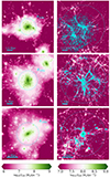 |
Fig. 1. Projected DM density maps of three simulated clusters at z = 0 (left column), with total masses M200c = 2 × 10¹⁵ M⊙ (top), 9 × 10¹⁴ M⊙ (middle), and 2 × 10¹⁴ M⊙ (bottom), and their z = 2.2 progenitors (right column). The cyan circle at z = 0 traces the R200c radius of each cluster, the one at z = 2.2 defines the PC region as defined in the text. DM particles at z = 2.2 that collapse within the R200c radius by z = 0 are plotted in cyan. Densities are computed in pixels of size 15 kpc in the top panel and 10 kpc in the middle and bottom panels. |
We show the radius of the PC regions as defined above in Fig. 2, in units of R200c of the main progenitor halo, as a function of the final (z = 0) mass of the cluster. We also show in Fig. 2 the distance from the center of the defined PC region to the closest boundary of the high-resolution region, defined as the distance of the closest low-resolution DM particle from the center of the main progenitor halo. We point out that this is a conservative definition of the boundary of the high-resolution zoom-in region. In fact, few low-resolution DM particles could spuriously be present within the regions where high-resolution particles are largely dominant. We verified that no such particles are present within the defined PCs, thus guaranteeing that the chaotic diffusion of low-resolution particles does not contaminate these regions.
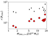 |
Fig. 2. Extension of the PC regions (in units of R200c of the main progenitor halos) at z = 2.2 as a function of the mass, M200c, of the descendant clusters at z = 0 (red diamonds). The downward arrows show, for each progenitor, the boundary of the high-resolution region (see main text). |
As expected, there is a correlation between the extension of the PC radius and the final mass of the cluster it will collapse into, reflecting the hierarchical build-up of structures. On the other hand, the arbitrariness of the PC center for large systems, such as the one shown in the top panel of Fig. 1, produces an artificial increase of the sphere’s radius for more massive systems.
Figure 3 shows the projected maps of stellar mass densities in the progenitors of two example clusters, with M200c = 5 × 10¹⁴ M⊙ and 2 × 10¹⁵ M⊙ at z = 0. Both regions are characterized by filaments of galaxies intersecting each other at the locations where massive halos are emerging.
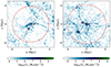 |
Fig. 3. Projected stellar mass density maps of two DIANOGA PC regions, which are the progenitors of clusters of total mass M200c equal to 5 × 10¹⁴ M⊙ and 2 × 10¹⁵ M⊙ at z = 0 (left and right panel, respectively). In each panel, the larger red dashed circle corresponds to the PC region as defined in the text, while the smaller circles show the R200c of halos in these regions with M200c > 1013 M⊙. Densities are computed in pixels of size 15 (10) kpc in the right (left) panel. |
In this work, we analyzed the properties of simulated PC galaxies and compared them with analogs at the same redshift in a reference, average density region. To this purpose, we used the population of galaxies identified within a cosmological box with size 49 cMpc/h per side, simulated with the same version of OpenGADGET3, assuming the same cosmology and subgrid models for baryonic physics. To have the same mass resolution as the DIANOGA zoom-in regions, initial conditions were generated for 5763 DM particles and as many gas particles. In this box, two cluster-size halos of masses M200c = 1.8 and 1.7 × 10¹⁴ M⊙ are present at z = 0; however, we did not exclude their progenitors from the analysis of the galaxy population, following the “field” definition adopted in observational studies, which refers to a large, representative volume, with all the possible overdense structures it contains.
2.3. Photometric properties of simulated galaxies
In this section we describe the radiation transfer simulations we performed to produce dust-attenuated spectral energy distributions (SEDs) for the simulated PC galaxies. These were used to analyze rest-frame UVJ color-color diagrams, and in particular compare the results of this widely used photometric classification of star-forming and quenched galaxies in observational studies (e.g., Labbé et al. 2005; Williams et al. 2009) with the classification based on their intrinsic properties in the simulations. A proper comparison with the UVJ photometric classification approach requires accounting for the effect of the extinction produced by dust on the UV/optical/NIR emission associated with the stellar populations in the simulated galaxies. We resorted to the Monte Carlo radiation transfer code SKIRT-92 (Camps & Baes 2020) for this purpose. The simulations that we analyzed here do not include a self-consistent treatment for the generation and evolution of dust grains. However, this can be implemented and indeed has been done in a lower-resolution version of these simulations (see Gjergo et al. 2018, for details). Therefore, we modeled the dust distribution through the spatial distribution of metals in the gas component of the simulated galaxies by adopting a fixed dust-to-metal ratio, for which we used the value fDTM = 0.2 (e.g., Trčka et al. 2022). To each SPH gas particle, with mass mgas and metallicity Z (fraction of mass in metals), was then attributed a dust mass equal to mdust = fDTM Z mgas.
We adopted the THEMIS model (Jones et al. 2017) to assign a composition and grain size distribution to dust in the ISM, with associated optical properties that are based on laboratory measurements of materials physically similar to interstellar dust. To discretize the simulation physical domain, in terms of properties of the absorbing medium, we adopted an oct-tree structure (e.g., Saftly et al. 2013). In this kind of grid, cubic meshes are recursively split to half their linear size, thus generating eight “child nodes” each, until they meet a convergence criterion in the last “leaves” of the tree3. In each cell of the final grid, the properties of the medium (dust) and of the radiation field originating from the sources, represented by star particles of the hydrodynamical simulations, are considered uniform. The stellar emission is modeled by approximating each star particle as a simple stellar population (SSP), consistent with the stellar evolution model included in the DIANOGA simulations. For each SSP we adopted a Bruzual & Charlot (2003, BC03) SED, which was specified by its age, initial mass and metallicity, as predicted by the simulations, once a Chabrier (2003) IMF was assumed.
The self-consistent treatment described above does not account for age-dependent extinction (e.g., Silva et al. 1998; Granato et al. 2001), with young stars highly attenuated by the remnants of their high-opacity birth clouds on spatial scales that are not resolved by the cosmological simulations. To gauge the impact of age-dependent dust extinction on our results, we also ran simulations with SKIRT, including a model for molecular clouds (MCs) and the self-consistent treatment of the diffuse ISM described above. We followed Granato et al. (2021) but adopted a higher age threshold of 10 Myr to select stars still affected by their birth cloud, as in Baes et al. (2024). To model the extinction of young stars, we placed them all at the center of an idealized macro-MC with a fixed M/r2 ratio, where M is the molecular gas mass, which we approximated with the total mass of the “cold” gas phase of the ISM (SH03) of each galaxy, and r is its radius. Indeed, it can be shown that assuming all young stars to be embedded in one large MC with a given opacity and extracting their cumulative SED is equivalent to considering them singularly attenuated by MCs of the same opacity and then summing over their SEDs. To assign an opacity to the macro-MC, we started from Silva et al. (1998), who showed that the M/r2 ratio, and not the single values of M and r, determines the opacity of MCs. Then, we constrained the radius of the idealized MC by adopting the same M/r2 ratio of a giant MC with a mass of molecular gas equal to 106 M⊙ and a radius of 15 pc, as done in Granato et al. (2021). Then, the dust mass in this cloud was given by Mdust, MC = fc fDTM Zc Mgas, where fc is the fraction of cold gas in each galaxy, as predicted by our cosmological hydrodynamical simulations, Zc is the metallicity of the cold component of the ISM and Mgas is the total gas mass. For consistency, we removed the cold gas assigned to the MCs from the diffuse medium that produces the attenuation of the emission of older star particles by multiplying the mass of each gas particle (therefore of each dust particle) by 1 − fc. SEDs of individual galaxies were then computed by summing the SEDs of the old and young star populations.
In both the runs with and without a model for MCs, we ran SKIRT in extinction-only mode, where calculations on the dust thermal re-emission at IR wavelengths are omitted to speed up the computations. We defer to future work a full exploration of the parameter space concerning the sub-resolution modeling of MCs, which is beyond the purpose of this analysis. In Sect. 3.5 we show that the conclusions presented in this work are not affected by the modeling of MCs.
3. Results
3.1. Properties of protocluster halos
In this section we present the properties of the population of halos in DIANOGA PCs, specifically focusing on their masses and characteristic radii. We compared these properties with those of observed halos associated with PCs or high-z clusters, which we used as a reference for comparing the simulated galaxy population properties in the following sections. Additionally, we examined the velocity dispersion of their member galaxies to provide a more complete comparison with dynamically inferred masses and to identify potential sources of discrepancy in such estimates. Indeed, velocity dispersions are commonly used in dynamical studies of observed halos as proxies for their total masses, assuming spherical symmetry and local relaxation. In the simulated PCs, we considered all halos with M200c > 1013 M⊙, and calculated the 1D velocity dispersions of galaxies identified within the 3D R200c of each halo, along three orthogonal lines of sight.
We show the results of this analysis in Fig. 4, where the masses M200c are plotted as a function of the galaxy velocity dispersions along the three lines of sight. These results are compared with observational estimates for (proto)clusters at z ∼ 2 − 2.5 from Gobat et al. (2013), Shimakawa et al. (2014), Wang et al. (2016, 2018), Mantz et al. (2018) and Di Mascolo et al. (2023). The estimates from Shimakawa et al. (2014) for the Spiderweb PC at z = 2.2 and the two subgroups of USS1558-003 at z = 2.53, within their estimated R200c, come from a dynamical analysis based on velocity dispersions. The remaining data include estimates based on observations of the intracluster medium (ICM): X-ray data for CLJ1001 at z = 2.5 (Wang et al. 2016, in agreement with estimates based on stellar mass and velocity dispersions), XLSSC 122 at z = 1.98 (Mantz et al. 2018; Willis et al. 2020; Noordeh et al. 2021), and ClJ1449 at z = 2.00 (Gobat et al. 2013; Valentino et al. 2016; Strazzullo et al. 2018), as well as estimates from the Sunyaev–Zeldovich (SZ) signal for the Spiderweb PC (Di Mascolo et al. 2023, consistent with X-ray measurements from Tozzi et al. 2022a). Wherever needed, we convert M500c to M200c (and R500c to R200c) using the relations from Ragagnin et al. (2021).
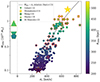 |
Fig. 4. Mass M200c of massive halos in PC regions as a function of velocity dispersion σv along three orthogonal lines of sight (represented by circles, squares and diamonds) as traced by galaxies with stellar masses larger than 109 M⊙ and lying within the R200c of each halo. Each point is color coded according to the halo R200c. The symbols with red contours mark the central halos of all PCs. The dashed curve represents the relation between dynamical masses and galaxy velocity dispersions calibrated in simulations by Saro et al. (2013) up to z = 1.2 and extrapolated at z = 2.2. Star symbols represent velocity dispersions and dynamical mass estimates within the core of the Spiderweb PC and for the two subgroups of USS1558-003 from Shimakawa et al. (2014). The cross symbol corresponds to CLJ1001 (Wang et al. 2016). The pentagon symbol shows M200c for the Spiderweb PC, from Sunyaev–Zeldovich effect measurements with the Atacama Large Millimeter/submillimeter Array (ALMA; Di Mascolo et al. 2023), the triangle represents the cluster XLSSC 122 (Mantz et al. 2018; Willis et al. 2020; Noordeh et al. 2021) and the downward triangle represents ClJ1449 (Gobat et al. 2013). These three points are shown artificially at σv < 0 since velocity dispersions measured consistently within the estimated radii are not available. |
We also show an analytic redshift-dependent relation between dynamical mass and velocity dispersion, calibrated by Saro et al. (2013) on simulations up to z = 1.2, and extrapolated to z = 2.2, in Fig. 4. In general, the simulated halos are in good agreement with this relation. For the few large halos with M200c ∼ 1014 M⊙, the figure suggests an increased scatter in velocity dispersions, though with very limited statistics. This might be due to the earlier stage of assembly of these objects. In such cases, the assumption of spherical symmetry underlying the definition of R200c may not be valid. The comparison with Shimakawa et al. (2014) shows good overlap with the mass and velocity dispersion ranges of the simulated halos studied here, with the Spiderweb PC core, lying at the high-mass end of our probed range, a factor ≲2 more massive than our most massive halos. On the other hand, this estimate of the Spiderweb PC core mass is a factor ∼3 larger than the ICM-based estimates (Tozzi et al. 2022a; Di Mascolo et al. 2023), which are well within the mass range of our simulated halos, as well as the other halos mentioned above.
The inconsistency between different observations of the same system is likely due to the complications of a dynamical analysis in highly disturbed systems, especially at these redshifts. Such analyses rely on the assumptions of local virialization, spherical symmetry, and the reliable removal of line-of-sight interlopers, all of which may bias the measurement of the velocity dispersion.
With these caveats, we conclude that our PC regions are populated with halos similar in mass and velocity dispersion (when available) to clusters and PC cores identified in observations at z ∼ 2 − 2.5.
3.2. Galaxy stellar mass function
The galaxy stellar mass function is an important observable in constraining galaxy formation models since it is essentially the integrated star formation history in a given region. In cosmological simulations, the GSMF at various redshifts is often used to fine-tune parameters of sub-resolution models related to the ISM and star formation processes. However, in the DIANOGA simulations, no tuning has been applied to the evolution of the GSMF, making it a genuine prediction. In this section we present the simulated GSMF and investigate its environmental dependence by selecting galaxies from different regions within the PCs and in the cosmological box. We also compared the simulated GSMF with observed GSMFs in PCs at z ∼ 2 − 2.5, in order to assess whether our simulations can reproduce the integrated star formation history observed in these systems.
The simulated GSMF for DIANOGA PCs is shown in Fig. 5. To highlight environmental signatures associated with the most massive halos (cores) in the PC regions, we separately considered galaxies hosted by halos with M200c > 1.5 × 10¹³ M⊙ in PCs. This separation is intended to investigate differences between galaxy populations in PC cores and those in the extended PC structure. The specific threshold of M200c = 1.5 × 10¹³ M⊙ corresponds to the mean mass of the third most massive progenitor halo, with the median mass ratio between first and third most massive progenitors at this redshift being 3.5. We show the predicted GSMF for PC cores, for the extended PC regions4 and for the cosmological box. The GSMF normalization is obviously higher in denser regions; the GSMFs shown in Fig. 5 have been rescaled to highlight differences in their shape.
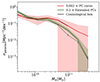 |
Fig. 5. Galaxy stellar mass functions in the PC environment compared with the cosmological box. The red line is the median of the GSMFs in PC cores, with and without central galaxies (solid and dashed lines, respectively; we note that the dashed line stops at M* ∼ 1011 M⊙ because the median GSMF in PC cores in the higher mass bins is zero when central galaxies are excluded). The green line shows the median GSMF in the less dense, diffuse PC regions, masking out all PC cores. The normalizations have been rescaled by the factors reported in the legend. The shaded regions define the 16th–84th percentile range spanned by the different PCs (or PC cores). The black line is the GSMF in the cosmological box, with Poissonian uncertainties. |
The comparison between the GSMFs in the cosmological box and in the extended PC regions reveals a slight relative excess of massive galaxies, with M* > 1010 M⊙, in the latter. This indicates that even when excluding galaxies in large halos, PCs exhibit a faint signature of accelerated evolution at earlier times. As expected, the excess of massive galaxies is more pronounced for the median GSMF in PC cores. This signal is completely dominated by central galaxies at M* ≳ 1011 M⊙. This result is qualitatively consistent with recent observational findings, such as the top-heavy feature in the GSMF of CLJ1001 at z = 2.5 (Sun et al. 2024) and the large ratio of high-mass to low-mass galaxies relative to the field in the Elentári proto-supercluster at z ∼ 3.3 (Forrest et al. 2024). We note that the GSMF of PC cores shows significant variability at high stellar masses among different cores, with a considerable scatter toward low number densities at M* ≳ 5 × 10¹⁰ M⊙, which seems to be primarily due to the lower-mass PC cores not having formed a significant fraction of massive galaxies yet. We note that the presence of massive halos in the cosmological box does not impact the global properties of the galaxy population. We identified the three most massive halos, with M200c in the range (1−3) × 1013 M⊙, in the cosmological box and defined a PC region around each of them, assuming an extent of 6.5 times their R200c (the average radius of the DIANOGA PCs with similar descendant mass). The galaxies within such regions comprise only 4% of the total galaxy population within the box, and their presence has only a negligible effect on the GSMF.
In Fig. 6 we compare the predicted GSMF with observations in PCs at similar redshift, including the Spiderweb PC (Pannella et al., in prep.), CLJ1001 (Sun et al. 2024) and 14 PCs identified in the COSMOS field at 2 < z < 2.5 (Edward et al. 2024). We tried to replicate the selection of the observational data as closely as possible for an accurate comparison between simulations and observations. For the comparison with Pannella et al. (in prep.) and Sun et al. (2024), we computed the GSMF within the same projected area covered by the observations and apply a redshift cut (including the contribution from peculiar motions) equivalent to the one imposed by the narrow-band filters in the data. Edward et al. (2024) use photometric redshifts with statistical subtraction of the background, meaning that the actual extension of the probed PC regions along the line of sight is unconstrained. As a result, for comparison to this work we only matched the projected area of these observations and rescaled their GSMF fit by a factor of 10 to approximately match the normalization of the simulated GSMF. For each simulation, we repeated the selection along three orthogonal lines of sight, extracting the median across all 3 × 14 realizations of the GSMF and computed the 16th–84th percentiles to define the scatter among simulated PCs. We applied a convolution with a Gaussian distribution of errors in the logarithm of stellar masses, with a dispersion of 0.3 dex, to approximate observational uncertainties (e.g., Conroy 2013; Mobasher et al. 2015; Lower et al. 2020). For Sun et al. (2024), we show the sum of the observed GSMFs of star-forming and quenched galaxies, although the latter is affected by incompleteness.
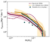 |
Fig. 6. Comparison between the GSMF in DIANOGA PCs and in observations of PCs at z ∼ 2 − 2.5 (Spiderweb, CLJ1001, 14 PCs in the COSMOS field; Pannella et al., in prep.; Sun et al. 2024; Edward et al. 2024, respectively). For each set of observations, a simulated GSMF has been produced to match the selection of galaxies as closely as possible. For each selection, GSMFs have been extracted along three orthogonal lines of sight, convolved with Gaussian errors with scatter 0.3 dex (see text), and the solid lines (shaded regions) show the median GSMFs (16th–84th percentile ranges, respectively) across all realizations, in the same color as the corresponding data. |
This comparison highlights an overall agreement in the normalization of the GSMF with observations (excluding Edward et al. 2024, where the normalization has been arbitrarily rescaled as mentioned above). The shape of the simulated GSMF is in very good agreement with Edward et al. (2024) and consistent with Pannella et al. (in prep.) especially at high masses (we note that these observations may suffer from significant incompleteness at lower stellar masses; see Tozzi et al. 2022b). On the other hand, we do not reproduce the strong top-heavy feature observed in the GSMF in CLJ1001 (Sun et al. 2024).
3.3. Star-forming main sequence
The star-forming MS is a key observable for constraining the mode of star formation as a function of stellar mass at different epochs. As such, it is useful to highlight the effect of environment on the star formation activity of galaxies. However, theoretical models continue to struggle to match the normalization of the observed MS at cosmic noon, with most semi-analytic models and cosmological simulation suites underestimating galaxy SFRs at high redshift (see, e.g., Granato et al. 2015; Hirschmann et al. 2016; Donnari et al. 2019; Akins et al. 2022; Andrews et al. 2024; Fontanot et al. 2024), despite the fact that simulations can be tuned to reproduce the observed GSMFs quite well. Star formation has been investigated in lower-resolution versions of the DIANOGA simulations, showing indeed lower SFRs of galaxies in PCs with respect to the observed MS (e.g., Bassini et al. 2020) and a star formation history that is not sufficiently bursty and thus is unable to reproduce FIR observations in high-z PCs (Granato et al. 2015).
In the following, we compared the star-forming MS in the DIANOGA PCs and in the cosmological box at z = 2.2 to investigate the impact of environment on the population of star-forming galaxies, and we compared these results with observations both in the field and in PCs. We classified galaxies as star forming if their specific SFR (sSFR) exceeds 0.3/tH (where tH is the Hubble time at z = 2.2; Franx et al. 2008). Figure 7 shows that this threshold appropriately separates star-forming and quenched galaxies in our simulations, falling approximately 1 dex below the peak of the simulated MS and intersecting the sSFR distribution at the point where quenched galaxies lead to a change in the slope of the distribution, both in the PCs and the cosmological box.
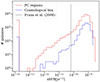 |
Fig. 7. Distributions of sSFRs of galaxies in the DIANOGA PC regions (red line) and in the cosmological box (blue line) at z = 2.2 compared with the threshold separating star-forming from quenched galaxies, at this redshift, from Franx et al. (2008). Galaxies with SFR = 0 have been artificially assigned the minimum non-zero sSFR, corresponding to 10−14 yr−1. |
In Fig. 8 we compare the simulated MS with observational data for PCs and the field at the same redshift. Specifically, we compare the median SFRs, as a function of stellar mass, across all the simulated PCs and in the cosmological box with observations in the Spiderweb PC from Pannella et al. (in prep., with SFR measurements based on dust-corrected rest-frame UV fluxes) and Pérez-Martínez et al. (2023, with Hα-based SFRs), and with field measurements from Schreiber et al. (2015, based on Herschel observations). To ensure a more proper comparison with these observations, we computed the SFRs of simulated galaxies averaged over 200 Myr, which is approximately the timescale of the SFR tracers used in Pannella et al. (in prep.) and in Schreiber et al. (2015), while Hα observations used in Pérez-Martínez et al. (2023) trace an almost instantaneous SFR, with the relevant timescales being 5−10 Myr. We show in Fig. B.1 that the SFRs in the cosmological box and in the PCs at z = 2.2 decline over the past 200 Myr in our simulations, with instantaneous SFRs systematically lower than averaged ones across all probed stellar masses. Nevertheless, the offset between these two SFRs estimates (∼0.1 dex on average) is much smaller than typical observational uncertainties. Therefore, considering also the limited sample sizes in MS investigations in observed high-z PCs, we expect the comparison between simulated and observed SFRs in Fig. 8 not to be affected by the different timescales of the mentioned SFR tracers, and thus we used SFRs averaged over 200 Myr in Fig. 8 and in the following.
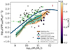 |
Fig. 8. Star-forming MS of galaxies in the DIANOGA PCs (orange) and in the cosmological box (green). Solid lines define the median SFRs of all star-forming galaxies within each stellar mass bin, while the shaded areas mark the 16th–84th percentile intervals. The star symbols represent proto-BCGs identified in the simulations, color coded according to the mass M200c of the main progenitor halo of each PC. Black diamonds and green dots are data for the Spiderweb PC from Pannella et al. (in prep.) and from Pérez-Martínez et al. (2023), respectively. The blue line is the best fit for the observed field star-forming MS by Schreiber et al. (2015) at z = 2.2. The red bar shows the estimated SFRs for the Spiderweb galaxy from measurements by Seymour et al. (2012) and Drouart et al. (2014). Simulated SFRs are averaged over 200 Myr (see text). |
The simulated MS is systematically lower than the observed one, both in the field and in the Spiderweb PC. The 11 star-forming proto-BCGs5 also have lower SFRs compared to the Spiderweb galaxy. A similar underestimation of SFRs at high redshift is present also in lower-resolution simulations of the DIANOGA PCs (Granato et al. 2015; Ragone-Figueroa et al. 2018; Bassini et al. 2020), which also adopt different prescriptions for the feedback processes. This suggests that the primary cause for the lower MS normalization predicted by simulations lies in the star formation model (SH03), which uses a quiescent mode of star formation that inherently prevents any bursty star formation episodes, which are instead expected at cosmic noon.
Ragone-Figueroa et al. (2024) show that by adopting a different model for star formation and stellar feedback (Murante et al. 2010, 2015; Valentini et al. 2020, 2023), coupled with H2 formation on dust grains (Granato et al. 2021), the discrepancy between the simulated and observed MS can be reduced, also resulting in a cosmic star formation history that better matches the observed one.
Within the simulation, we observe that less massive PC main progenitors host proto-BCGs with suppressed star formation compared to the (simulated) MS. The simulated MS in Fig. 8 also shows a rather minor suppression of star formation in PCs compared to the cosmological box6. This is further explored in Fig. 9 where, for a better understanding of the effect of the environment, we separated star-forming galaxies hosted by PC cores (M200c > 1.5 × 10¹³ M⊙) from those in the lower-density extended regions of PCs, comparing them also with galaxies in the cosmological box.
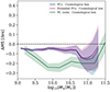 |
Fig. 9. Environmental dependence of the simulated star-forming MS at z = 2.2 as a function of stellar mass. Results are shown for the whole sample of PC galaxies, as well as separating PC galaxies located within/outside R200c of halos with M200c > 1.5 × 10¹³ M⊙ (PC cores), comparing them to results for the cosmological box. The solid lines and shaded regions show the MS offset and its uncertainty between pairs of environments as indicated in the legend (see text for details). |
Figure 9 shows the environmental dependence of the star-forming MS by comparing offsets in SFRs between the aforementioned galaxy populations. To compute the offsets, we generated 1000 realizations of the MS of each galaxy population, assuming an (asymmetric) Gaussian distribution of SFRs as a function of stellar mass based on the median SFR and 16th–84th percentile range for the given population of simulated galaxies. For each population (and thus environment) pair, we then computed the mean of the SFR offsets as a function of stellar mass over these 1000 realizations. The error on the offset is estimated as the scatter of the SFR offsets across the realizations.
We predict a very small though significant suppression of approximately 0.05 dex in the SFRs of PC galaxies compared to the cosmological box (we note that this is insensitive to including or excluding the most massive halos, as their galaxy populations are subdominant compared to the full PC structure). This suppression is independent of stellar mass, though for log10(M*/M⊙) > 11 statistical uncertainties are too large to draw any conclusions. The observational uncertainties in the current MS determinations do not allow the detection of a 0.05 dex offset. Therefore, this prediction from simulations is compatible with studies that found either a low-significance or no suppression in the SFRs of PC galaxies compared to their field counterparts (e.g., Cucciati et al. 2014; Koyama et al. 2021; Polletta et al. 2021; Shi et al. 2021; Pérez-Martínez et al. 2023). On the other hand, our predicted offset contrasts with other studies finding an enhanced star formation in PC galaxies (e.g., Pannella et al., in prep.; Shimakawa et al. 2018; Monson et al. 2021; Pérez-Martínez et al. 2024).
Figure 9 further shows that the star formation suppression is more significant in PC cores, with an MS offset up to ∼0.25 dex compared to the cosmological box. This offset decreases to ∼0.05 dex for galaxies with M* ∼ 109 M⊙. For these galaxies, whose star formation history has experienced a more marked recent decline (see Fig. B.1), the SFR averaged over 200 Myr may be less sensitive to their relatively rapid evolution, especially in PC cores, as is discussed in the following.
Given that star formation in the DIANOGA simulations depends on the gas reservoir and on the efficiency of gas conversion into stars, we further explored how these quantities compare with observational constraints. The reservoir of star-forming gas is represented by the cold component of the multi-phase gas particles that describe the ISM in the SH03 star formation model adopted in our simulations (see Sect. 2.1). We computed the cold gas fraction, μcold = Mcold/M*, where Mcold is the total cold gas mass in a galaxy. We compared this cold gas fraction with the molecular gas fraction, Mmolecular/M*, which is estimated in observational investigations, noting that Mcold represents an upper limit to the (sub-resolution) molecular gas content. We also computed the depletion time tdep = Mcold/SFR, using the SFR averaged over 200 Myr.
In Fig. 10 we show μcold and tdep as a function of stellar mass for star-forming galaxies, both in PCs and in the cosmological box, comparing them with observational results from Magdis et al. (2012), Liu et al. (2019), Sanders et al. (2023), Mérida et al. (2024) and Leroy et al. (2024) at z ∼ 1.5 − 3. In both PCs and the cosmological box, our simulations predict cold gas fractions that are systematically lower than the observed values, while the depletion times (thus the star formation efficiencies) appear consistent with observations. However, considering the realistic GSMF in the simulated PCs discussed in Sect. 3.2, the cold gas deficit suggests a possible inefficiency in gas cooling, excessive heating due to feedback processes, or highly efficient interactions with the hot ambient gas, which begins to permeate the simulated halos at these redshifts (Esposito et al., in prep.), rather than an early over-consumption of gas.
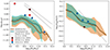 |
Fig. 10. Cold gas fractions (left panel) and depletion times (right panel) in star-forming galaxies in the DIANOGA PCs (orange) and in the cosmological box (green) as a function of stellar masses. Solid lines (shaded regions) show median values (16th–84th percentile ranges, respectively). For comparison, we show observations at z ∼ 1.5 − 3 from Magdis et al. (2012), Liu et al. (2019), Sanders et al. (2023), Mérida et al. (2024) and Leroy et al. (2024). |
As shown in Fig. 10, the fraction of cold gas is slightly lower in PCs than in the cosmological box. To investigate this further, we derived offsets in the median cold gas fraction and depletion times of galaxies in PCs in comparison with galaxies in the cosmological box, as a function of stellar mass, using the same methodology applied for the MS offsets in Fig. 9. The resulting offsets are shown in Fig. 11. For the cold gas fraction, we observe a small (∼0.05 dex) though significant suppression in the cold gas reservoir in PC galaxies across all stellar masses, similar to the trends seen for the MS. For star-forming galaxies in PC cores, the offset in μcold relative to the cosmological box decreases at lower masses, suggesting a more efficient depletion or less efficient replenishment of gas in low-mass galaxies. Since this feature is specific to the most massive halos in the PC regions, it is possible that interactions with the hot ICM emerging in these massive halos are either stripping cold gas from galaxies or halting cosmological gas accretion, leading to more rapid gas depletion, especially in lower-mass galaxies. In particular, the offset in μcold shows a sharp drop at log(M*/M⊙)≲9.5. This is because approximately 40% of galaxies in this mass range within PC cores, classified as star forming based on their averaged SFRs, have completely lost their cold gas reservoir, effectively shutting off star formation over the past 200 Myr. While these galaxies are in a regime where the results could be influenced by the finite numerical resolution of the simulations, galaxies of similar mass in the cosmological box and in smaller halos within the PC regions do not show such an abrupt decrease in cold gas fractions. Therefore, we conclude that this is not a numerical artifact, although the extreme environment in the largest halos within the simulated PC regions, coupled with the relatively low number of gas particles in galaxies with log(M*) < 9.5, may amplify a genuine physical process occurring in massive halos at this redshift. Figure 11 also shows that the environmental dependence of depletion times qualitatively mirrors the trends observed for the cold gas fraction. The offset in the median depletion time of galaxies in the full PC region in comparison with the cosmological box (with no sensitivity to the inclusion or exclusion of the most massive halos) is marginal and statistically insignificant. However, low-mass PC galaxies within the most massive halos exhibit a dramatic decrease in their median depletion time, corresponding to the low median cold gas fractions discussed above.
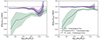 |
Fig. 11. Environmental dependence of the fraction of cold gas (left panel) and of the cold gas depletion time (right panel) at z = 2.2 as a function of stellar mass. Here we consider four environments: the cosmological box, the whole PCs, the low-density extended PCs and the PC cores. The solid lines define the offsets between the cold fractions and the depletion times in the PC environments with respect to the cosmological box, as defined in the legend, resulting from 1000 Monte Carlo realizations (see text). The shaded regions represent the intrinsic scatter on the offsets. |
3.4. Quenched galaxy fractions
In this section we analyze the population of quenched galaxies in the DIANOGA PCs and in the cosmological box at z = 2.2, to quantify how the environment of massive halos in PCs suppresses star formation in galaxies. This represents the first necessary step to exploit the simulations in probing the nature of early quenching processes in cluster progenitor environments, in the context of understanding the physical mechanisms resulting in the predominance of quenched galaxies in mature clusters at later epochs.
We investigated the effects of the local environment, by isolating galaxies hosted by PC cores of different halo masses and galaxies populating the extended PC structures. We also separated galaxies in two stellar mass bins (109 < M*/M⊙ < 1010 and M* > 1010 M⊙) to examine how galaxies of different masses are differently affected by the environment. The median quenched fractions as a function of halo mass, and the fractions in the wide PC structures and in the cosmological box, are shown in Fig. 12.
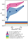 |
Fig. 12. Fraction of quenched galaxies in PC cores as a function of the core mass M200c in the DIANOGA PCs at z = 2.2. The dots are median quenched fractions across different cores in each mass bin and the shaded areas are the 16th–84th percentile ranges. The horizontal bands show the fraction of all quenched galaxies in the coeval cosmological box (its width is the 1σ confidence interval calculated following Cameron 2011), and the 16th–84th interval of quenched fractions in the PC extended regions (masking out the PC cores), across the 14 different simulations, independently of their host halo mass. Results are shown for galaxies with stellar masses in the range 109 < M*/M⊙ < 1010 and M* > 1010 M⊙ separately. |
Across all stellar masses, the quenched galaxy fraction increases significantly in more massive halos, reaching up to 90% (70%) for the 109 < M*/M⊙ < 1010 (M* > 1010 M⊙) galaxy population at M200c ≥ 1014 M⊙. The scatter around the median is representative of the halo-to-halo variation, though higher halo mass bins might be affected by limited statistics.
The DIANOGA simulations predict an increased efficiency of quenching mechanisms compared to the cosmological box, across all the probed stellar mass and halo mass ranges, already at z = 2.2. Noticeably, the fractions of quenched galaxies in the extended PC regions exceed those in the cosmological box, suggesting that star formation in galaxies might be suppressed before their infall into the virial region of a massive halo.
While these simulations predict an increasing quenched fraction as a function of stellar mass in the cosmological box and in the extended PC regions, in qualitative agreement with field observations (e.g., Muzzin et al. 2013; Kawinwanichakij et al. 2017; Sherman et al. 2020; Park et al. 2024), we note that Fig. 12 shows instead higher quenched fractions for 109 < M*/M⊙ < 1010 than for M* > 1010 M⊙ galaxies in PC cores, at odds with observations in the field, as mentioned above, as well as in observed clusters and PCs (e.g., van der Burg et al. 2013, 2020; Cooke et al. 2016; Lee-Brown et al. 2017; Edward et al. 2024). This issue is common in various cosmological simulation suites across different redshifts, stellar masses, and environments (e.g. Bahé et al. 2017; Donnari et al. 2021). This discrepancy is likely a direct consequence of the over-consumption of gas in low-mass star-forming galaxies, as is discussed in Sect. 3.3 and further investigated in a forthcoming study.
In Fig. 13 we compare the quenched galaxy fraction in the most massive PC cores, with M200c > 5 × 10¹³ M⊙, with observations in similar environments at z ∼ 2 − 2.5, including XLSSC 122 (Willis et al. 2020; Noordeh et al. 2021), CLJ1001 (Wang et al. 2016) and ClJ1449 (Gobat et al. 2011; Strazzullo et al. 2018). We note that, while the quoted quenched fractions for XLSSC 122 and CLJ1001 are computed in very similar apertures (approximately 600 and 700 kpc, respectively) and the two (proto)clusters have similar halo masses (M200c ∼ 8−9 × 10¹³ M⊙), the quoted quenched fraction in ClJ1449 (with M200c ∼ 5 × 10¹³ M⊙) is computed within a much smaller aperture of 200 kpc. To compare the quenched fractions in simulated PCs with these observations, we selected galaxies in the same apertures and with stellar masses larger than the completeness limits in the referenced observational studies. We thus stress that measurements in different stellar mass bins shown in Fig. 13 are not homogeneous in terms of the size of the considered region around the PC centers. We also compare the quenched fractions in the cosmological box with field observations in COSMOS/UltraVISTA (Muzzin et al. 2013) and in CANDELS/3D-HST (Skelton et al. 2014) at z ∼ 2 − 2.5. For completeness, we also show the quenched fractions in the PC cores in the highest stellar mass bin, even though there is no direct comparison with observed PCs. We calculated these quenched fractions, as a reference, within the average R200c (440 kpc) of the considered halos. The massive halos in the simulated PCs exhibit a broad range of quenched galaxy fractions, reflecting the diversity in the timing of evolutionary processes affecting galaxies in overdense environments at cosmic noon. In particular, the most star forming among massive PC cores show fractions of quenched galaxies comparable to those in the cosmological box as do observed PCs with negligible environmental quenching (e.g., CLJ1001, Wang et al. 2016), while the most quiescent PC cores resemble the most mature observed systems (e.g., XLSSC 122, Noordeh et al. 2021)7. Quenched fractions in the cosmological box in the stellar mass range probed in Fig. 13 are close to observed quenched fractions in the field at similar redshift, especially at M* ∼ 4−5 × 10¹⁰ M⊙, whereas at higher (lower) masses they are slightly overestimated (underestimated).
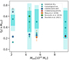 |
Fig. 13. Comparison of quenched fractions in the most massive simulated PC cores (with M200c ≥ 5 × 10¹³ M⊙) and observations at z ∼ 2 − 2.5. We note that measurements in this figure are not homogeneous in terms of the size of the considered region around the PC center (see text). The cyan dots show the median quenched fractions among selected halos, while shaded dark (light) regions are the 16th–84th percentile (minimum-maximum) ranges. The cyan diamonds, with binomial population uncertainties (Cameron 2011), are quenched fractions extracted from the cosmological box. For comparison with the observations in CLJ1001, XLSSC 122 and ClJ1449, galaxies in PCs were selected above a limiting stellar mass (Mlim) and within a physical aperture around halo centers, matching those adopted in Wang et al. (2016), Noordeh et al. (2021) and Strazzullo et al. (2018), respectively (see text for details). For comparison with the cosmological box, we also show the quenched fractions in the field from COSMOS/UltraVISTA catalog (Muzzin et al. 2013) and from the CANDELS/3D-HST survey (Skelton et al. 2014) at 2 < z < 2.5. |
Based on results from these simulations, the large scatter observed in the quenched fraction of PC cores is primarily driven by intrinsic variability in the evolutionary phase of PC cores of similar mass at z ∼ 2. We also note that the quenched fractions of galaxies in the innermost regions of massive PC cores, as shown in comparison with ClJ1449, have the largest scatter. While the intrinsic variability might indeed be enhanced in the selected innermost region of massive halos, the increased scatter might also be due to lower statistics in such small volumes. A more detailed investigation of the processes affecting galaxy evolution in halos of different masses and at different halo-centric radii will be presented in Esposito et al. (in prep.).
3.5. UVJ diagrams
In observational studies, UVJ diagrams are widely used to classify galaxies as star forming or quenched (e.g., Labbé et al. 2005; Williams et al. 2009; Whitaker et al. 2012). Donnari et al. (2019) found that the fractions of quenched galaxies inferred from UVJ diagrams in the IllustrisTNG simulations were consistent with those estimated from the galaxy distance from the MS at redshifts 0 ≤ z ≤ 2, by adopting a separation line between star-forming and quenched galaxies that preserves the slope of the commonly used classification (e.g., Whitaker et al. 2011), but is shifted to account for the slightly different color distribution compared to observations. We tested this approach in the DIANOGA simulations, coupled with the SKIRT-9 radiative transfer code (see Sect. 2.3), to investigate potential complications in the comparison between galaxy populations in simulations and observations, particularly in the context of high-redshift massive halos.
We produced UVJ diagrams for a random sample of seven massive halos, with M200c=(0.6−1.4) × 1014 M⊙, in our simulations. We selected galaxies with M* > 2 × 10¹⁰ M⊙, which is approximately the mass range that can be reasonably probed with mass-complete samples in deep observational investigations of z ∼ 2 PC galaxy populations thus far, and located within a 3D aperture radius of 700 kpc from the center of each halo, corresponding to ∼1.5 × R200c. The resulting UVJ diagrams are shown in Fig. 14. The two panels refer to results based on two models, corresponding to including or not a prescription for MCs (see Sect. 2.3). In the following, we refer to these two models as “diffuse model” (left panel) and “MC model” (right panel), respectively. We note that the diffuse model relies on a smaller number of assumptions and represents a more direct prediction of the simulations, though it does not resolve the scales of MCs.
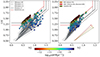 |
Fig. 14. Simulated UVJ diagrams for galaxies within seven massive halos in DIANOGA PC regions at z = 2.2, within a 700 kpc aperture, produced with SKIRT-9. Intrinsic colors are connected to attenuated colors by gray arrows that end with star symbols color coded according to the sSFRs of galaxies. The left panel shows the diagram obtained by tracing dust in the diffuse ISM through a fixed dust-to-metal ratio. The right panel shows the diagram produced with the model for MCs described in Sect. 2.3. Typical cuts adopted in UVJ diagrams to separate quenched and star-forming galaxies (Williams et al. 2009; Whitaker et al. 2011, 2012; Muzzin et al. 2013) are shown as black lines, while the red line defines a custom-defined boundary to separate these populations in the DIANOGA simulations. The colored arrows show the reddening vectors for typical attenuation laws (Allen 1976; Prevot et al. 1984; Bouchet et al. 1985; Calzetti et al. 2000). |
The diagrams for both models reveal that galaxy populations in the simulated halos exhibit a red sequence (e.g., Bell et al. 2004) that is already in place at z = 2.2, reflecting the high quenched fractions presented in Sect. 3.4. These red galaxies form a tight sequence in the quenched region of the diagram and are largely unaffected by dust attenuation, due to the limited gas reservoir in quenched galaxies, which translates into little dust to absorb the stellar emission in our modeling. Qualitatively, the distribution of both quenched and star-forming galaxies is in agreement with observed UVJ diagrams. However, the actual color distribution of the simulated star-forming galaxies is not the same as for observed counterparts. Therefore, to quantitatively match the separation between the two galaxy populations based on their sSFR (see Fig. 7), we needed to shift the separation line by approximately 0.2 mag toward redder U-V colors compared to standard separations used in the literature (e.g., Williams et al. 2009; Whitaker et al. 2011, 2012; Muzzin et al. 2013). We note that this is in quantitative agreement with the UVJ separation found by Donnari et al. (2019) in the IllustrisTNG simulations, as well as with the color distributions in SIMBA simulations at z = 2 from Akins et al. (2022).
For star-forming galaxies, the diffuse model produces overall stronger attenuation (the average AV for the studied sample is 1, compared with 0.5 for the MC model), which is dominated by the attenuation of the diffuse dust on the more abundant older stellar population. In this respect, we recall that the MC model subtracts the cold gas reservoir from the total gas contributing to the attenuation of older stars in the ISM. Since star-forming galaxies in PCs reach very high fractions of cold to total gas, this leaves overall a rather small amount of diffuse gas, and consequently dust, in the MC model, resulting in lower dust attenuation compared to the diffuse model. The details of this effect are related to the assumptions adopted in the MC model implemented here, however, as discussed in Sect. 2.3, tuning this model is not the focus of this analysis; our primary interest in modeling the age-dependent attenuation of MCs is understanding its qualitative influence on the reddening of galaxy colors in the UVJ diagrams.
Figure 14 shows that, in our modeling of dust attenuation applied to DIANOGA simulations (diffuse model), the majority of the galaxy population has reddening vectors in agreement with typical attenuation laws (e.g., Allen 1976; Prevot et al. 1984; Bouchet et al. 1985; Calzetti et al. 2000). However, a subset of star-forming galaxies exhibit steeper reddening vectors. This is consistent with the results from Akins et al. (2022) on SIMBA simulations coupled with dust radiative transfer. In fact, they found that the assumption of a universal Calzetti et al. (2000) attenuation law might impact the efficacy of the UVJ classification, especially for star-forming galaxies near the quenched region of the UVJ diagram. This leads to the incorrect classification of these galaxies as quenched when applying standard UVJ cuts (Williams et al. 2009; Whitaker et al. 2011, 2012; Muzzin et al. 2013). This behavior appears in both our models. Thus, although the MC model seems to extend this feature to a larger fraction of the galaxy population compared to the diffuse model, this is not a numerical artifact introduced by our modeling. We note that the galaxies that are characterized by such “atypical” steep reddening vectors tend to be central galaxies or at least located very close to them and have high stellar masses (≳ 1011 M⊙). The comparison between the two models suggests that the limited resolution of cosmological simulations, which cannot capture the high densities typical of MCs, does not explain this inconsistency in the simulated UVJ diagram. Indeed, if anything, the MC model produces a more pronounced tilt of the reddening vector in the UVJ plane.
We investigated the “atypical” galaxies further by analyzing the spatial distributions of their stars and metals (whose mass is mapped into dust mass in our modeling) and their star formation histories. As an example, we show in Fig. 15 these quantities for one of these galaxies. The star formation history (right panel) shows approximately constant SFR for the last ∼2 Gyr at ∼400 M⊙ yr−1. The distribution of stars (left panel) shows a positive gradient of stellar ages, while the distribution of metals (central panel) is concentrated in a dense central core. The steepness of the reddening vector is thus produced by the presence of a central population of young stars that are highly attenuated by the core of high-metallicity gas. This is a genuine signal of age-dependent extinction produced by the simulations (though at larger scales than the unresolved MCs), which causes a stronger reddening of the U-V color than of the V-J color (see Fig. 14).
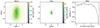 |
Fig. 15. Properties of a galaxy characterized by a steep reddening vector. The left panel shows the distribution of stars, color coded according to their age, while the middle panel shows the distribution of gas particles color coded according to their mass in metals, both within 0.25 kpc from the center of the galaxy along the line of sight. The right panel shows the galaxy star formation history. |
4. Summary and conclusions
In this study, we have analyzed the properties of galaxy populations in PCs at z = 2.2 in the DIANOGA set of zoom-in cosmological hydrodynamical simulations of galaxy clusters. These include 14 re-simulations of galaxy clusters originally selected in a DM-only simulation box of size 1 cGpc/h. Alongside the PC simulations, we also analyzed a cosmological box of 49 cMpc/h per side representing an average region of the Universe that was simulated at the same resolution and with the same galaxy formation model in terms of sub-resolution descriptions of the relevant astrophysical processes.
To define PCs in simulations, we traced back the DM that falls within the R200c of the z = 0 cluster and identified, around the most massive progenitor halo, a region that encompasses 80% of all these DM particles. In all of our analyses, we considered galaxies with M* > 109 M⊙ to ensure an adequate numerical resolution.
We investigated the properties of simulated galaxy populations and we compared them to observations to test the predictions of simulations, focusing on halos with properties similar to the observed (proto)cluster cores. We compared galaxy properties in the simulated PCs and in the cosmological box to highlight the impact of environment on galaxy evolution, as predicted by our simulations. We also performed radiative transfer simulations using the SKIRT-9 code (Camps & Baes 2020) to estimate dust-attenuated rest-frame UV to NIR colors of simulated galaxies, by consistently tracing dust through metals in the gas component, and we tested the impact of adopting a UVJ photometric classification of star-forming and quenched galaxies, as routinely applied in observational studies. We summarize our main conclusions as follows.
-
The GSMF in the DIANOGA PCs is broadly consistent with observations in PCs at 2 ≤ z ≤ 2.5, both in shape and normalization (see Fig. 6). This demonstrates that the integrated star formation history in the simulated PCs realistically reproduces the observational data. The median PC GSMF reveals an excess of galaxies with M* > 1010 M⊙ compared to the cosmological box (see Fig. 5). This excess is detected both in PC cores (M200c > 1.5 × 10¹³ M⊙) and, albeit with lower significance, in the extended PC regions (i.e., outside the cores). Since this excess is indicative of early stellar mass assembly, its presence in the extended PC regions suggests the onset of an overall accelerated galaxy evolution in the broader environments hosting PCs.
-
The SFRs of star-forming galaxies in both the PCs and the cosmological box are lower than expected from observations (see Fig. 8). This is consistent with previous results from lower-resolution versions of the DIANOGA simulations (Granato et al. 2015; Bassini et al. 2020) and other suites of cosmological hydrodynamical simulations (e.g., Akins et al. 2022; Andrews et al. 2024). The SFRs in PC galaxies show a small (∼0.05 dex) yet significant suppression compared to galaxies in the cosmological box (see Fig. 9). This signal is dominated by galaxies in the extended structures of the PCs, while galaxies in the PC cores exhibit a more pronounced suppression (up to ∼0.25 dex lower SFRs compared to the cosmological box).
-
The reservoirs of cold star-forming gas are systematically lower than observational estimates at z ∼ 1.5 − 3, while depletion times are broadly consistent with those observed in star-forming galaxies, both in the PCs and in the cosmological box (see Fig. 10). This suggests that the underestimation of SFRs in the simulations is related to galaxies not having sufficient gas available to convert into stars, possibly due to the effect of a too efficient feedback inhibiting cooling or expelling gas. Protocluster galaxies in our simulations have marginally lower cold gas content than their counterparts in the cosmological box on average, while depletion times do not show significant differences (see Fig. 11). However, galaxies in PC cores exhibit more marked differences in both cold gas fractions and depletion times compared to galaxies in the extended PC structure and in the cosmological box. In massive cores, both cold gas fractions and depletion times show a significant drop for galaxies with log10(M*) < 9.5, and they remain significantly lower than the cosmological box levels at higher masses. This is due to a large fraction (∼40%) of galaxies with log10(M*/M⊙) < 9.5 that are classified as star forming based on their SFR averaged over the past 200 Myr but have actually completely lost their cold gas over this time. We note that these galaxies may be in a regime influenced by the finite numerical resolution. However, since galaxies of similar mass in other simulated regions do not show such a sudden loss of gas, this feature could reflect a genuine physical process emerging in simulated massive halos at high redshift, possibly amplified by the combined effect of relatively limited numerical resolution and the extreme environment of the most massive high-z halos.
-
The fraction of quenched galaxies in the simulations increases significantly with the mass of the host halo in the PC cores, reaching approximately 0.9 (0.7) at M200c ≥ 1014 M⊙ for galaxies with 109 < M*/M⊙ < 1010 (M* > 1010 M⊙, respectively; see Fig. 12). Our simulations predict an increasing fraction of quenched galaxies toward lower stellar masses in PC cores, which is at odds with indications from observations (e.g., Muzzin et al. 2013; van der Burg et al. 2013, 2020; Cooke et al. 2016; Lee-Brown et al. 2017; Kawinwanichakij et al. 2017; Sherman et al. 2020; Park et al. 2024; Edward et al. 2024) and with our predictions in the cosmological box and outside the cores of the simulated PCs. This trend is common to many suites of cosmological simulations (e.g., Bahé et al. 2017; Donnari et al. 2021). The fraction of quenched galaxies in PCs, even outside massive cores, is higher than in the cosmological box, implying accelerated quenching also in lower-density PC regions before infall into massive halos.
-
The DIANOGA PCs include halos in which quenching has progressed in very different ways (see Figs. 12, 13), similar to the observed PCs. In some halos, the galaxy quenched fraction is as low as in the cosmological box (comparable to observed starbursting PC cores, e.g., CLJ1001 at z = 2.51, Wang et al. 2016), while in others it is as high as in observed mature clusters (e.g., XLSSC 122 at z = 1.98, Willis et al. 2020; Noordeh et al. 2021). The quenched fractions in the cosmological box also qualitatively agree with observations in the field.
-
We found that the distribution of galaxies in the simulated UVJ diagram in a sample of 7 massive simulated halos is qualitatively consistent with observed distributions of star-forming and quenched galaxies (see Fig. 14). However, from a more quantitative point of view, we needed to shift the UVJ selection boundary by 0.2 mag toward redder U-V colors, compared to typical classification criteria used in observations, to optimally match the sSFR-based classification of our simulated galaxies. Despite the overall qualitative agreement, we note indeed the presence of a population of star-forming galaxies (mainly massive galaxies in the central regions of PC cores) with a steep reddening vector, leading to significant contamination of the quenched region of the diagram when adopting standard selections.
In this work, we have demonstrated that the DIANOGA cosmological hydrodynamical simulations can broadly reproduce the properties of galaxy populations in observed PCs at z ∼ 2 − 2.5, which is a particularly significant time for the evolution of clusters and their host galaxies since it corresponds to the transition between PC structures and the first established clusters. This redshift range also corresponds to a cosmic epoch where the cosmic SFR density is at its peak and, at the same time, the first signatures of environmental quenching appear in the densest environments. We show that the environment of cluster progenitors has an impact on galaxy populations, particularly through the early onset and subsequent suppression of star formation, which is most significant in the massive PC cores. These results provide an interpretative framework that consistently accounts for the full cosmological context for understanding the evolution of galaxies in PCs.
The next crucial step is to constrain when, where, and how the environment of (proto)clusters affects the evolution of galaxy populations considering the broad range of environments that these galaxies cross throughout their evolutionary history. This includes investigating the buildup of the diffuse ICM that permeates mature clusters as well as examining internal processes within galaxies, including AGN activity.
The results of our analysis highlight that the current generation of cosmological hydrodynamical simulations are invaluable instruments to shed light on the complex interplay between environment and the physical processes that shape galaxy evolution. In this respect, cluster progenitor environments at cosmic noon present a significant challenge to models of star formation and feedback processes, as they couple extreme regions of the Universe and a cosmic time where transformational processes are at their peak. In this context, and while keeping in mind the current limitations that still affect the comparison of observations and simulations at high redshift, our findings highlight the need for improved modeling of galaxy formation and evolution to better capture observed galaxy population properties (the level of star formation in particular) in the densest high-redshift regions. This is a crucial part of the broader effort to consistently reproduce the evolution of galaxy populations across cosmic time and across different environments.
We note that the adopted cosmology differs from the fiducial flat ΛCDM and the standard Planck 2018 (Planck Collaboration VI 2020) cosmologies adopted in recent observational studies. However, we verified that the impact of cosmology on halo masses, stellar masses and radii is well within typical statistical and systematic uncertainties in current observations.
We considered boxes of 64 kpc per side encompassing each galaxy and chose, for the construction of the oct-tree, a maximum fraction of the total dust mass in a leaf equal to 8 × 10⁻⁷, and a maximum number of refinement levels equal to seven, corresponding to a minimum size of leaf nodes equal to the gravitational softening of the gas component in the simulations.
To calculate the GSMFs of PC cores we used the volume of the sphere with the radius R200c of each halo, while for the extended PCs we used the radius of the PC region as defined in Sect. 2.2, to which we subtract the cumulative volume occupied by the PC cores.
We define as proto-BCG the central galaxy of the main progenitor halo in each PC. 3 out of 14 proto-BCGs, also shown in Fig. 8, are quenched, according to our definition.
We verified that masking the “PC” regions in the cosmological box, as defined above, does not impact this result.
We estimate the mass completeness limit based on the spectroscopic completeness limit from Willis et al. (2020), assuming a BC03 SSP with formation redshift z = 5 and no dust.
Acknowledgments
We thank Luca Tornatore for technical support, Alice Damiano for useful discussion, and an anonymous referee for constructive comments that helped improve the presentation of the results. Simulations have been carried out at the CINECA Italian Supercomputing Center, with computational resources allocated through an ISCRA-B proposal. This paper is supported by: the Italian Research Center on High Performance Computing, Big Data and Quantum Computing (ICSC), project funded by European Union – NextGenerationEU – and National Recovery and Resilience Plan (NRRP) – Mission 4 Component 2, within the activities of Spoke 3, Astrophysics and Cosmos Observations; by the National Recovery and Resilience Plan (NRRP), Mission 4, Component 2, Investment 1.1, Call for tender No. 1409 published on 14.9.2022 by the Italian Ministry of University and Research (MUR), funded by the European Union – NextGenerationEU – Project Title “Space-based cosmology with Euclid: the role of High-Performance Computing” – CUP J53D23019100001 – Grant Assignment Decree No. 962 adopted on 30/06/2023 by the Italian Ministry of University and Research (MUR); by the PRIN 2022 (20225E4SY5) “From ProtoClusters to Clusters in one Gyr”; by the INAF Astrofisica Fondamentale GO Grant 2022 “Environmental quenching efficiency across the virial volume of the most massive, most distant clusters”; by the INAF Astrofisica Fondamentale Large Grant 2023 “Witnessing the Birth of the Most Massive Structures of the Universe”. We acknowledge partial financial support from the INFN Indark Grant, from the Consejo Nacional de Investigaciones Científicas y Técnicas (CONICET) (PIP-2021-11220200102832CO), from the Agencia Nacional de Promoción de la Investigación, el Desarrollo Tecnológico y la Innovación de la República Argentina (PICT-2020-03690), and from the European Union’s HORIZON-MSCA-2021-SE-01 Research and Innovation Programme under the Marie Sklodowska-Curie grant agreement number 101086388 – Project (LACEGAL).
References
- Akins, H. B., Narayanan, D., Whitaker, K. E., et al. 2022, ApJ, 929, 94 [NASA ADS] [CrossRef] [Google Scholar]
- Allen, C. W. 1976, Astrophysical Quantities (London: The Athlone Press) [Google Scholar]
- Andreon, S., Maughan, B., Trinchieri, G., & Kurk, J. 2009, A&A, 507, 147 [NASA ADS] [CrossRef] [EDP Sciences] [Google Scholar]
- Andrews, M., Artale, M. C., Kumar, A., et al. 2024, ArXiv e-prints [arXiv:2410.08412] [Google Scholar]
- Angulo, R. E., Springel, V., White, S. D. M., et al. 2012, MNRAS, 425, 2722 [NASA ADS] [CrossRef] [Google Scholar]
- Baes, M., Gebek, A., Trčka, A., et al. 2024, A&A, 683, A181 [NASA ADS] [CrossRef] [EDP Sciences] [Google Scholar]
- Bahé, Y. M., Barnes, D. J., Dalla Vecchia, C., et al. 2017, MNRAS, 470, 4186 [Google Scholar]
- Bassini, L., Rasia, E., Borgani, S., et al. 2020, A&A, 642, A37 [NASA ADS] [CrossRef] [EDP Sciences] [Google Scholar]
- Bell, E. F., Wolf, C., Meisenheimer, K., et al. 2004, ApJ, 608, 752 [NASA ADS] [CrossRef] [Google Scholar]
- Bonafede, A., Dolag, K., Stasyszyn, F., Murante, G., & Borgani, S. 2011, MNRAS, 418, 2234 [NASA ADS] [CrossRef] [Google Scholar]
- Bouchet, P., Lequeux, J., Maurice, E., Prevot, L., & Prevot-Burnichon, M. L. 1985, A&A, 149, 330 [NASA ADS] [Google Scholar]
- Bruzual, G., & Charlot, S. 2003, MNRAS, 344, 1000 [NASA ADS] [CrossRef] [Google Scholar]
- Cai, Z., Fan, X., Peirani, S., et al. 2016, ApJ, 833, 135 [NASA ADS] [CrossRef] [Google Scholar]
- Cai, Z., Fan, X., Bian, F., et al. 2017, ApJ, 839, 131 [NASA ADS] [CrossRef] [Google Scholar]
- Calzetti, D., Armus, L., Bohlin, R. C., et al. 2000, ApJ, 533, 682 [NASA ADS] [CrossRef] [Google Scholar]
- Cameron, E. 2011, PASA, 28, 128 [Google Scholar]
- Camps, P., & Baes, M. 2020, Astron. Comput., 31, 100381 [NASA ADS] [CrossRef] [Google Scholar]
- Chabrier, G. 2003, PASP, 115, 763 [Google Scholar]
- Clements, D. L., Braglia, F. G., Hyde, A. K., et al. 2014, MNRAS, 439, 1193 [NASA ADS] [CrossRef] [Google Scholar]
- Conroy, C. 2013, ARA&A, 51, 393 [NASA ADS] [CrossRef] [Google Scholar]
- Cooke, E. A., Hatch, N. A., Stern, D., et al. 2016, ApJ, 816, 83 [NASA ADS] [CrossRef] [Google Scholar]
- Cucciati, O., Zamorani, G., Lemaux, B. C., et al. 2014, A&A, 570, A16 [NASA ADS] [CrossRef] [EDP Sciences] [Google Scholar]
- Cucciati, O., Lemaux, B. C., Zamorani, G., et al. 2018, A&A, 619, A49 [NASA ADS] [CrossRef] [EDP Sciences] [Google Scholar]
- Daddi, E., Jin, S., Strazzullo, V., et al. 2017, ApJ, 846, L31 [Google Scholar]
- Damiano, A., Valentini, M., Borgani, S., et al. 2024, A&A, 692, A81 [NASA ADS] [CrossRef] [EDP Sciences] [Google Scholar]
- Di Mascolo, L., Saro, A., Mroczkowski, T., et al. 2023, Nature, 615, 809 [NASA ADS] [CrossRef] [Google Scholar]
- Dolag, K., Borgani, S., Murante, G., & Springel, V. 2009, MNRAS, 399, 497 [Google Scholar]
- Donnari, M., Pillepich, A., Nelson, D., et al. 2019, MNRAS, 485, 4817 [Google Scholar]
- Donnari, M., Pillepich, A., Nelson, D., et al. 2021, MNRAS, 506, 4760 [NASA ADS] [CrossRef] [Google Scholar]
- Drouart, G., De Breuck, C., Vernet, J., et al. 2014, A&A, 566, A53 [NASA ADS] [CrossRef] [EDP Sciences] [Google Scholar]
- Edward, A. H., Balogh, M. L., Bahé, Y. M., et al. 2024, MNRAS, 527, 8598 [Google Scholar]
- Eisenhardt, P. R. M., Brodwin, M., Gonzalez, A. H., et al. 2008, ApJ, 684, 905 [Google Scholar]
- Elbaz, D., Dickinson, M., Hwang, H. S., et al. 2011, A&A, 533, A119 [NASA ADS] [CrossRef] [EDP Sciences] [Google Scholar]
- Fontanot, F., De Lucia, G., Xie, L., et al. 2024, A&A, submitted [arXiv:2409.02194] [Google Scholar]
- Forrest, B., Lemaux, B. C., Shah, E. A., et al. 2024, ApJ, 971, 169 [NASA ADS] [Google Scholar]
- Franx, M., van Dokkum, P. G., Förster Schreiber, N. M., et al. 2008, ApJ, 688, 770 [NASA ADS] [CrossRef] [Google Scholar]
- Gaspari, M., Eckert, D., Ettori, S., et al. 2019, ApJ, 884, 169 [NASA ADS] [CrossRef] [Google Scholar]
- Gjergo, E., Granato, G. L., Murante, G., et al. 2018, MNRAS, 479, 2588 [NASA ADS] [CrossRef] [Google Scholar]
- Gobat, R., Daddi, E., Onodera, M., et al. 2011, A&A, 526, A133 [NASA ADS] [CrossRef] [EDP Sciences] [Google Scholar]
- Gobat, R., Strazzullo, V., Daddi, E., et al. 2013, ApJ, 776, 9 [NASA ADS] [CrossRef] [Google Scholar]
- Granato, G. L., Silva, L., Bressan, A., et al. 2001, Astrophys. Space Sci. Suppl., 277, 79 [Google Scholar]
- Granato, G. L., Ragone-Figueroa, C., Domínguez-Tenreiro, R., et al. 2015, MNRAS, 450, 1320 [NASA ADS] [CrossRef] [Google Scholar]
- Granato, G. L., Ragone-Figueroa, C., Taverna, A., et al. 2021, MNRAS, 503, 511 [NASA ADS] [CrossRef] [Google Scholar]
- Greenslade, J., Clements, D. L., Cheng, T., et al. 2018, MNRAS, 476, 3336 [NASA ADS] [CrossRef] [Google Scholar]
- Groth, F., Steinwandel, U. P., Valentini, M., & Dolag, K. 2023, MNRAS, 526, 616 [NASA ADS] [CrossRef] [Google Scholar]
- Guaita, L., Pompei, E., Castellano, M., et al. 2020, A&A, 640, A107 [NASA ADS] [CrossRef] [EDP Sciences] [Google Scholar]
- Haines, C. P., Pereira, M. J., Smith, G. P., et al. 2015, ApJ, 806, 101 [NASA ADS] [CrossRef] [Google Scholar]
- Hatch, N. A., Kurk, J. D., Pentericci, L., et al. 2011, MNRAS, 415, 2993 [NASA ADS] [CrossRef] [Google Scholar]
- Hirschmann, M., De Lucia, G., & Fontanot, F. 2016, MNRAS, 461, 1760 [Google Scholar]
- Ito, K., Tanaka, M., Valentino, F., et al. 2023, ApJ, 945, L9 [NASA ADS] [CrossRef] [Google Scholar]
- Jones, A. P., Köhler, M., Ysard, N., Bocchio, M., & Verstraete, L. 2017, A&A, 602, A46 [NASA ADS] [CrossRef] [EDP Sciences] [Google Scholar]
- Kawinwanichakij, L., Papovich, C., Quadri, R. F., et al. 2017, ApJ, 847, 134 [NASA ADS] [CrossRef] [Google Scholar]
- Koyama, Y., Polletta, M. D. C., Tanaka, I., et al. 2021, MNRAS, 503, L1 [NASA ADS] [CrossRef] [Google Scholar]
- Labbé, I., Huang, J., Franx, M., et al. 2005, ApJ, 624, L81 [Google Scholar]
- Lee, K.-G., Hennawi, J. F., Stark, C., et al. 2014, ApJ, 795, L12 [NASA ADS] [CrossRef] [Google Scholar]
- Lee-Brown, D. B., Rudnick, G. H., Momcheva, I. G., et al. 2017, ApJ, 844, 43 [Google Scholar]
- Lemaux, B. C., Le Fèvre, O., Cucciati, O., et al. 2018, A&A, 615, A77 [NASA ADS] [CrossRef] [EDP Sciences] [Google Scholar]
- Leroy, L., Elbaz, D., Magnelli, B., et al. 2024, A&A, 691, A248 [NASA ADS] [CrossRef] [EDP Sciences] [Google Scholar]
- Lim, S., Scott, D., Babul, A., et al. 2021, MNRAS, 501, 1803 [Google Scholar]
- Lim, S., Tacchella, S., Schaye, J., et al. 2024, MNRAS, 532, 4551 [NASA ADS] [CrossRef] [Google Scholar]
- Liu, D., Schinnerer, E., Groves, B., et al. 2019, ApJ, 887, 235 [Google Scholar]
- Lower, S., Narayanan, D., Leja, J., et al. 2020, ApJ, 904, 33 [NASA ADS] [CrossRef] [Google Scholar]
- Magdis, G. E., Daddi, E., Béthermin, M., et al. 2012, ApJ, 760, 6 [NASA ADS] [CrossRef] [Google Scholar]
- Magorrian, J., Tremaine, S., Richstone, D., et al. 1998, AJ, 115, 2285 [Google Scholar]
- Mantz, A. B., Abdulla, Z., Allen, S. W., et al. 2018, A&A, 620, A2 [NASA ADS] [CrossRef] [EDP Sciences] [Google Scholar]
- Mantz, A. B., Allen, S. W., Morris, R. G., et al. 2020, MNRAS, 496, 1554 [NASA ADS] [CrossRef] [Google Scholar]
- Marini, I., Borgani, S., Saro, A., et al. 2021, MNRAS, 507, 5780 [NASA ADS] [CrossRef] [Google Scholar]
- McConachie, I., Wilson, G., Forrest, B., et al. 2022, ApJ, 926, 37 [NASA ADS] [CrossRef] [Google Scholar]
- McConnell, N. J., & Ma, C.-P. 2013, ApJ, 764, 184 [Google Scholar]
- Mérida, R. M., Gómez-Guijarro, C., Pérez-González, P. G., et al. 2024, A&A, 686, A64 [NASA ADS] [CrossRef] [EDP Sciences] [Google Scholar]
- Miller, T. B., Chapman, S. C., Aravena, M., et al. 2018, Nature, 556, 469 [CrossRef] [Google Scholar]
- Mobasher, B., Dahlen, T., Ferguson, H. C., et al. 2015, ApJ, 808, 101 [NASA ADS] [CrossRef] [Google Scholar]
- Monson, E. B., Lehmer, B. D., Doore, K., et al. 2021, ApJ, 919, 51 [NASA ADS] [CrossRef] [Google Scholar]
- Murante, G., Monaco, P., Giovalli, M., Borgani, S., & Diaferio, A. 2010, MNRAS, 405, 1491 [NASA ADS] [Google Scholar]
- Murante, G., Monaco, P., Borgani, S., et al. 2015, MNRAS, 447, 178 [NASA ADS] [CrossRef] [Google Scholar]
- Muzzin, A., Marchesini, D., Stefanon, M., et al. 2013, ApJ, 777, 18 [NASA ADS] [CrossRef] [Google Scholar]
- Noeske, K. G., Weiner, B. J., Faber, S. M., et al. 2007, ApJ, 660, L43 [CrossRef] [Google Scholar]
- Noordeh, E., Canning, R. E. A., Willis, J. P., et al. 2021, MNRAS, 507, 5272 [NASA ADS] [CrossRef] [Google Scholar]
- Oteo, I., Ivison, R. J., Dunne, L., et al. 2018, ApJ, 856, 72 [Google Scholar]
- Overzier, R. A. 2016, A&ARv, 24, 14 [Google Scholar]
- Papovich, C., Momcheva, I., Willmer, C. N. A., et al. 2010, ApJ, 716, 1503 [NASA ADS] [CrossRef] [Google Scholar]
- Park, M., Belli, S., Conroy, C., et al. 2024, ApJ, 976, 72 [Google Scholar]
- Pentericci, L., McCarthy, P. J., Röttgering, H. J. A., et al. 2001, ApJS, 135, 63 [Google Scholar]
- Pérez-Martínez, J. M., Dannerbauer, H., Kodama, T., et al. 2023, MNRAS, 518, 1707 [Google Scholar]
- Pérez-Martínez, J. M., Kodama, T., Koyama, Y., et al. 2024, MNRAS, 527, 10221 [Google Scholar]
- Planck Collaboration VI. 2020, A&A, 641, A6 [NASA ADS] [CrossRef] [EDP Sciences] [Google Scholar]
- Polletta, M., Soucail, G., Dole, H., et al. 2021, A&A, 654, A121 [NASA ADS] [CrossRef] [EDP Sciences] [Google Scholar]
- Prevot, M. L., Lequeux, J., Maurice, E., Prevot, L., & Rocca-Volmerange, B. 1984, A&A, 132, 389 [Google Scholar]
- Ragagnin, A., Saro, A., Singh, P., & Dolag, K. 2021, MNRAS, 500, 5056 [Google Scholar]
- Ragone-Figueroa, C., Granato, G. L., Ferraro, M. E., et al. 2018, MNRAS, 479, 1125 [NASA ADS] [Google Scholar]
- Ragone-Figueroa, C., Granato, G. L., Parente, M., et al. 2024, A&A, 691, A200 [NASA ADS] [CrossRef] [EDP Sciences] [Google Scholar]
- Rasia, E., Borgani, S., Murante, G., et al. 2015, ApJ, 813, L17 [Google Scholar]
- Remus, R.-S., Dolag, K., & Dannerbauer, H. 2023, ApJ, 950, 191 [NASA ADS] [CrossRef] [Google Scholar]
- Saftly, W., Camps, P., Baes, M., et al. 2013, A&A, 554, A10 [NASA ADS] [CrossRef] [EDP Sciences] [Google Scholar]
- Sanders, R. L., Shapley, A. E., Jones, T., et al. 2023, ApJ, 942, 24 [NASA ADS] [CrossRef] [Google Scholar]
- Santos, J. S., Fassbender, R., Nastasi, A., et al. 2011, A&A, 531, L15 [NASA ADS] [CrossRef] [EDP Sciences] [Google Scholar]
- Saro, A., Borgani, S., Tornatore, L., et al. 2009, MNRAS, 392, 795 [NASA ADS] [CrossRef] [Google Scholar]
- Saro, A., Mohr, J. J., Bazin, G., & Dolag, K. 2013, ApJ, 772, 47 [NASA ADS] [CrossRef] [Google Scholar]
- Schreiber, C., Pannella, M., Elbaz, D., et al. 2015, A&A, 575, A74 [NASA ADS] [CrossRef] [EDP Sciences] [Google Scholar]
- Scoville, N., Arnouts, S., Aussel, H., et al. 2013, ApJS, 206, 3 [Google Scholar]
- Seymour, N., Altieri, B., De Breuck, C., et al. 2012, ApJ, 755, 146 [NASA ADS] [CrossRef] [Google Scholar]
- Sherman, S., Jogee, S., Florez, J., et al. 2020, MNRAS, 499, 4239 [Google Scholar]
- Shi, K., Toshikawa, J., Lee, K.-S., et al. 2021, ApJ, 911, 46 [NASA ADS] [CrossRef] [Google Scholar]
- Shimakawa, R., Kodama, T., Tadaki, K. I., et al. 2014, MNRAS, 441, L1 [NASA ADS] [CrossRef] [Google Scholar]
- Shimakawa, R., Kodama, T., Hayashi, M., et al. 2018, MNRAS, 473, 1977 [NASA ADS] [CrossRef] [Google Scholar]
- Silva, L., Granato, G. L., Bressan, A., & Danese, L. 1998, ApJ, 509, 103 [Google Scholar]
- Skelton, R. E., Whitaker, K. E., Momcheva, I. G., et al. 2014, ApJS, 214, 24 [Google Scholar]
- Smail, I. 2024, MNRAS, 529, 2290 [Google Scholar]
- Spitler, L. R., Labbé, I., Glazebrook, K., et al. 2012, ApJ, 748, L21 [NASA ADS] [CrossRef] [Google Scholar]
- Springel, V. 2005, MNRAS, 364, 1105 [Google Scholar]
- Springel, V., & Hernquist, L. 2003, MNRAS, 339, 289 [Google Scholar]
- Springel, V., White, S. D. M., Tormen, G., & Kauffmann, G. 2001, MNRAS, 328, 726 [Google Scholar]
- Springel, V., Di Matteo, T., & Hernquist, L. 2005, MNRAS, 361, 776 [Google Scholar]
- Staab, P., Lemaux, B. C., Forrest, B., et al. 2024, MNRAS, 528, 6934 [NASA ADS] [CrossRef] [Google Scholar]
- Steidel, C. C., Adelberger, K. L., Shapley, A. E., et al. 2000, ApJ, 532, 170 [NASA ADS] [CrossRef] [Google Scholar]
- Steinborn, L. K., Dolag, K., Hirschmann, M., Prieto, M. A., & Remus, R.-S. 2015, MNRAS, 448, 1504 [Google Scholar]
- Strazzullo, V., Daddi, E., Gobat, R., et al. 2015, A&A, 576, L6 [NASA ADS] [CrossRef] [EDP Sciences] [Google Scholar]
- Strazzullo, V., Coogan, R. T., Daddi, E., et al. 2018, ApJ, 862, 64 [NASA ADS] [CrossRef] [Google Scholar]
- Sun, H., Wang, T., Xu, K., et al. 2024, ApJ, 967, L34 [NASA ADS] [CrossRef] [Google Scholar]
- Tanaka, M., Onodera, M., Shimakawa, R., et al. 2024, ApJ, 970, 59 [Google Scholar]
- Thongkham, K., Gonzalez, A. H., Brodwin, M., et al. 2024, ApJ, 967, 123 [NASA ADS] [Google Scholar]
- Tormen, G. 1997, MNRAS, 290, 411 [NASA ADS] [CrossRef] [Google Scholar]
- Tornatore, L., Borgani, S., Dolag, K., & Matteucci, F. 2007, MNRAS, 382, 1050 [Google Scholar]
- Toshikawa, J., Kashikawa, N., Overzier, R., et al. 2016, ApJ, 826, 114 [NASA ADS] [CrossRef] [Google Scholar]
- Tozzi, P., Gilli, R., Liu, A., et al. 2022a, A&A, 667, A134 [NASA ADS] [CrossRef] [EDP Sciences] [Google Scholar]
- Tozzi, P., Pentericci, L., Gilli, R., et al. 2022b, A&A, 662, A54 [NASA ADS] [CrossRef] [EDP Sciences] [Google Scholar]
- Trčka, A., Baes, M., Camps, P., et al. 2022, MNRAS, 516, 3728 [CrossRef] [Google Scholar]
- Valentini, M., Murante, G., Borgani, S., et al. 2020, MNRAS, 491, 2779 [Google Scholar]
- Valentini, M., Dolag, K., Borgani, S., et al. 2023, MNRAS, 518, 1128 [Google Scholar]
- Valentino, F., Daddi, E., Finoguenov, A., et al. 2016, ApJ, 829, 53 [NASA ADS] [CrossRef] [Google Scholar]
- van der Burg, R. F. J., Muzzin, A., Hoekstra, H., et al. 2013, A&A, 557, A15 [NASA ADS] [CrossRef] [EDP Sciences] [Google Scholar]
- van der Burg, R. F. J., McGee, S., Aussel, H., et al. 2018, A&A, 618, A140 [NASA ADS] [CrossRef] [EDP Sciences] [Google Scholar]
- van der Burg, R. F. J., Rudnick, G., Balogh, M. L., et al. 2020, A&A, 638, A112 [NASA ADS] [CrossRef] [EDP Sciences] [Google Scholar]
- Wang, T., Elbaz, D., Daddi, E., et al. 2016, ApJ, 828, 56 [NASA ADS] [CrossRef] [Google Scholar]
- Wang, T., Elbaz, D., Daddi, E., et al. 2018, ApJ, 867, L29 [NASA ADS] [CrossRef] [Google Scholar]
- Whitaker, K. E., Labbé, I., van Dokkum, P. G., et al. 2011, ApJ, 735, 86 [Google Scholar]
- Whitaker, K. E., Kriek, M., van Dokkum, P. G., et al. 2012, ApJ, 745, 179 [CrossRef] [Google Scholar]
- Wiersma, R. P. C., Schaye, J., Theuns, T., Dalla Vecchia, C., & Tornatore, L. 2009, MNRAS, 399, 574 [NASA ADS] [CrossRef] [Google Scholar]
- Williams, R. J., Quadri, R. F., Franx, M., van Dokkum, P., & Labbé, I. 2009, ApJ, 691, 1879 [NASA ADS] [CrossRef] [Google Scholar]
- Willis, J. P., Canning, R. E. A., Noordeh, E. S., et al. 2020, Nature, 577, 39 [NASA ADS] [CrossRef] [Google Scholar]
- Wylezalek, D., Galametz, A., Stern, D., et al. 2013a, ApJ, 769, 79 [NASA ADS] [CrossRef] [Google Scholar]
- Wylezalek, D., Vernet, J., De Breuck, C., et al. 2013b, MNRAS, 428, 3206 [CrossRef] [Google Scholar]
- Zavala, J. A., Casey, C. M., Scoville, N., et al. 2019, ApJ, 887, 183 [NASA ADS] [CrossRef] [Google Scholar]
- Zheng, X. Z., Cai, Z., An, F. X., Fan, X., & Shi, D. D. 2021, MNRAS, 500, 4354 [Google Scholar]
Appendix A: Impact of apertures on stellar masses of simulated galaxies
Here we examine the impact of using stellar masses calculated within fixed apertures (2D, with an 8.5 kpc radius, corresponding to 1 arcsecond at z = 2.2) as opposed to using total SubFind masses. Figure A.1 shows the ratio of these two mass definitions as a function of aperture stellar mass. This ratio is ∼1 on average for stellar masses up to M* ∼ 1011 M⊙, with negligible scatter (∼0.005), for galaxies both in the PCs and in the cosmological box. For M* > 1011 M⊙, however, the deviation of the mass ratio from unity becomes significant, with the SubFind masses exceeding the aperture masses by a factor ∼1.3 (1.2) on average in the PCs (cosmological box, respectively).
Most galaxies (72%) with M* > 1011 M⊙ are central galaxies in massive halos, where SubFind fails to separate the galaxy from the diffuse stellar component (see, e.g., Marini et al. 2021). For M* > 1011 M⊙ satellites (which are thus not affected by this effect) the SubFind mass estimate still exceeds the aperture mass by a factor 1.1 on average, reaching up to a factor ≳2 for 1% of these most massive galaxies.
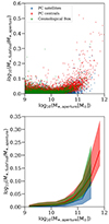 |
Fig. A.1. Ratio of SubFind and aperture stellar masses, as a function of aperture mass for galaxies in DIANOGA PCs, separated in centrals and satellites, and in the cosmological box at z = 2.2. Aperture masses are estimated within a two-dimensional projected radius equal to 8.5 kpc. The bottom panel shows the median (16th–84th percentiles) of the mass ratios of galaxies in the top panel, in solid lines (shaded areas, respectively). |
Appendix B: Effects of averaging SFRs
Here we assess differences between galaxy SFRs averaged over 200 Myr (SFR200), which more properly compare to some observational estimates used in this work (see Sect. 3.3), and the instantaneous SFRs associated with gas particles in the SH03 star formation model (SFRgas). Figure B.1 shows the ratio between these two SFR estimates as a function of stellar mass. SFRgas is lower than SFR200 across all the probed stellar mass range, with a weak increasing trend with increasing mass. Proto-BCGs behave similarly to other galaxies, with instantaneous SFRs tendentially lower than those averaged over the past 200 Myr. The same trends are observed in PCs and in the cosmological box, reflecting a declining star formation history of galaxies in both environments at z = 2.2, possibly more pronounced at lower masses.
Figure B.2 shows the distributions of specific SFRgas (SFR200) for galaxies in which the SFR200 (SFRgas, respectively) is zero, which are not accounted for in Fig. B.1. There are very few galaxies with SFR200 = 0 and SFRgas > 0, and their SFRgas corresponds anyway to a negligible level of residual star formation. Galaxies with SFRgas = 0 but SFR200 > 0 are more common; these galaxies have relatively low (averaged) sSFRs, with the bulk of them falling below the level of the adopted threshold for quenched galaxies. Galaxies for which both SFR estimates are zero also do not appear in Fig. B.1. However, they would in principle add to the population of galaxies for which the estimates are the same and, since they are a minority across all stellar masses, they would not significantly change the trend shown in Fig. B.1.
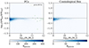 |
Fig. B.1. Two-dimensional histograms of the ratios of instantaneous SFR (SFRgas) and SFR averaged over 200 Myr (SFR200) of galaxies in DIANOGA PCs (left) and in the cosmological box (right) at z = 2.2, as a function of stellar mass. Proto-BCGs are plotted separately. |
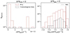 |
Fig. B.2. Distribution of the instantaneous (averaged) sSFRs for galaxies with SFR200 = 0 (SFRgas = 0), in the left (right, respectively) panel. The dashed lines show the average sSFR of main-sequence galaxies in the cosmological box (black) and in the PCs (red). |
All Tables
All Figures
|
Fig. 1. Projected DM density maps of three simulated clusters at z = 0 (left column), with total masses M200c = 2 × 10¹⁵ M⊙ (top), 9 × 10¹⁴ M⊙ (middle), and 2 × 10¹⁴ M⊙ (bottom), and their z = 2.2 progenitors (right column). The cyan circle at z = 0 traces the R200c radius of each cluster, the one at z = 2.2 defines the PC region as defined in the text. DM particles at z = 2.2 that collapse within the R200c radius by z = 0 are plotted in cyan. Densities are computed in pixels of size 15 kpc in the top panel and 10 kpc in the middle and bottom panels. |
| In the text | |
|
Fig. 2. Extension of the PC regions (in units of R200c of the main progenitor halos) at z = 2.2 as a function of the mass, M200c, of the descendant clusters at z = 0 (red diamonds). The downward arrows show, for each progenitor, the boundary of the high-resolution region (see main text). |
| In the text | |
|
Fig. 3. Projected stellar mass density maps of two DIANOGA PC regions, which are the progenitors of clusters of total mass M200c equal to 5 × 10¹⁴ M⊙ and 2 × 10¹⁵ M⊙ at z = 0 (left and right panel, respectively). In each panel, the larger red dashed circle corresponds to the PC region as defined in the text, while the smaller circles show the R200c of halos in these regions with M200c > 1013 M⊙. Densities are computed in pixels of size 15 (10) kpc in the right (left) panel. |
| In the text | |
|
Fig. 4. Mass M200c of massive halos in PC regions as a function of velocity dispersion σv along three orthogonal lines of sight (represented by circles, squares and diamonds) as traced by galaxies with stellar masses larger than 109 M⊙ and lying within the R200c of each halo. Each point is color coded according to the halo R200c. The symbols with red contours mark the central halos of all PCs. The dashed curve represents the relation between dynamical masses and galaxy velocity dispersions calibrated in simulations by Saro et al. (2013) up to z = 1.2 and extrapolated at z = 2.2. Star symbols represent velocity dispersions and dynamical mass estimates within the core of the Spiderweb PC and for the two subgroups of USS1558-003 from Shimakawa et al. (2014). The cross symbol corresponds to CLJ1001 (Wang et al. 2016). The pentagon symbol shows M200c for the Spiderweb PC, from Sunyaev–Zeldovich effect measurements with the Atacama Large Millimeter/submillimeter Array (ALMA; Di Mascolo et al. 2023), the triangle represents the cluster XLSSC 122 (Mantz et al. 2018; Willis et al. 2020; Noordeh et al. 2021) and the downward triangle represents ClJ1449 (Gobat et al. 2013). These three points are shown artificially at σv < 0 since velocity dispersions measured consistently within the estimated radii are not available. |
| In the text | |
|
Fig. 5. Galaxy stellar mass functions in the PC environment compared with the cosmological box. The red line is the median of the GSMFs in PC cores, with and without central galaxies (solid and dashed lines, respectively; we note that the dashed line stops at M* ∼ 1011 M⊙ because the median GSMF in PC cores in the higher mass bins is zero when central galaxies are excluded). The green line shows the median GSMF in the less dense, diffuse PC regions, masking out all PC cores. The normalizations have been rescaled by the factors reported in the legend. The shaded regions define the 16th–84th percentile range spanned by the different PCs (or PC cores). The black line is the GSMF in the cosmological box, with Poissonian uncertainties. |
| In the text | |
|
Fig. 6. Comparison between the GSMF in DIANOGA PCs and in observations of PCs at z ∼ 2 − 2.5 (Spiderweb, CLJ1001, 14 PCs in the COSMOS field; Pannella et al., in prep.; Sun et al. 2024; Edward et al. 2024, respectively). For each set of observations, a simulated GSMF has been produced to match the selection of galaxies as closely as possible. For each selection, GSMFs have been extracted along three orthogonal lines of sight, convolved with Gaussian errors with scatter 0.3 dex (see text), and the solid lines (shaded regions) show the median GSMFs (16th–84th percentile ranges, respectively) across all realizations, in the same color as the corresponding data. |
| In the text | |
|
Fig. 7. Distributions of sSFRs of galaxies in the DIANOGA PC regions (red line) and in the cosmological box (blue line) at z = 2.2 compared with the threshold separating star-forming from quenched galaxies, at this redshift, from Franx et al. (2008). Galaxies with SFR = 0 have been artificially assigned the minimum non-zero sSFR, corresponding to 10−14 yr−1. |
| In the text | |
|
Fig. 8. Star-forming MS of galaxies in the DIANOGA PCs (orange) and in the cosmological box (green). Solid lines define the median SFRs of all star-forming galaxies within each stellar mass bin, while the shaded areas mark the 16th–84th percentile intervals. The star symbols represent proto-BCGs identified in the simulations, color coded according to the mass M200c of the main progenitor halo of each PC. Black diamonds and green dots are data for the Spiderweb PC from Pannella et al. (in prep.) and from Pérez-Martínez et al. (2023), respectively. The blue line is the best fit for the observed field star-forming MS by Schreiber et al. (2015) at z = 2.2. The red bar shows the estimated SFRs for the Spiderweb galaxy from measurements by Seymour et al. (2012) and Drouart et al. (2014). Simulated SFRs are averaged over 200 Myr (see text). |
| In the text | |
|
Fig. 9. Environmental dependence of the simulated star-forming MS at z = 2.2 as a function of stellar mass. Results are shown for the whole sample of PC galaxies, as well as separating PC galaxies located within/outside R200c of halos with M200c > 1.5 × 10¹³ M⊙ (PC cores), comparing them to results for the cosmological box. The solid lines and shaded regions show the MS offset and its uncertainty between pairs of environments as indicated in the legend (see text for details). |
| In the text | |
|
Fig. 10. Cold gas fractions (left panel) and depletion times (right panel) in star-forming galaxies in the DIANOGA PCs (orange) and in the cosmological box (green) as a function of stellar masses. Solid lines (shaded regions) show median values (16th–84th percentile ranges, respectively). For comparison, we show observations at z ∼ 1.5 − 3 from Magdis et al. (2012), Liu et al. (2019), Sanders et al. (2023), Mérida et al. (2024) and Leroy et al. (2024). |
| In the text | |
|
Fig. 11. Environmental dependence of the fraction of cold gas (left panel) and of the cold gas depletion time (right panel) at z = 2.2 as a function of stellar mass. Here we consider four environments: the cosmological box, the whole PCs, the low-density extended PCs and the PC cores. The solid lines define the offsets between the cold fractions and the depletion times in the PC environments with respect to the cosmological box, as defined in the legend, resulting from 1000 Monte Carlo realizations (see text). The shaded regions represent the intrinsic scatter on the offsets. |
| In the text | |
|
Fig. 12. Fraction of quenched galaxies in PC cores as a function of the core mass M200c in the DIANOGA PCs at z = 2.2. The dots are median quenched fractions across different cores in each mass bin and the shaded areas are the 16th–84th percentile ranges. The horizontal bands show the fraction of all quenched galaxies in the coeval cosmological box (its width is the 1σ confidence interval calculated following Cameron 2011), and the 16th–84th interval of quenched fractions in the PC extended regions (masking out the PC cores), across the 14 different simulations, independently of their host halo mass. Results are shown for galaxies with stellar masses in the range 109 < M*/M⊙ < 1010 and M* > 1010 M⊙ separately. |
| In the text | |
|
Fig. 13. Comparison of quenched fractions in the most massive simulated PC cores (with M200c ≥ 5 × 10¹³ M⊙) and observations at z ∼ 2 − 2.5. We note that measurements in this figure are not homogeneous in terms of the size of the considered region around the PC center (see text). The cyan dots show the median quenched fractions among selected halos, while shaded dark (light) regions are the 16th–84th percentile (minimum-maximum) ranges. The cyan diamonds, with binomial population uncertainties (Cameron 2011), are quenched fractions extracted from the cosmological box. For comparison with the observations in CLJ1001, XLSSC 122 and ClJ1449, galaxies in PCs were selected above a limiting stellar mass (Mlim) and within a physical aperture around halo centers, matching those adopted in Wang et al. (2016), Noordeh et al. (2021) and Strazzullo et al. (2018), respectively (see text for details). For comparison with the cosmological box, we also show the quenched fractions in the field from COSMOS/UltraVISTA catalog (Muzzin et al. 2013) and from the CANDELS/3D-HST survey (Skelton et al. 2014) at 2 < z < 2.5. |
| In the text | |
|
Fig. 14. Simulated UVJ diagrams for galaxies within seven massive halos in DIANOGA PC regions at z = 2.2, within a 700 kpc aperture, produced with SKIRT-9. Intrinsic colors are connected to attenuated colors by gray arrows that end with star symbols color coded according to the sSFRs of galaxies. The left panel shows the diagram obtained by tracing dust in the diffuse ISM through a fixed dust-to-metal ratio. The right panel shows the diagram produced with the model for MCs described in Sect. 2.3. Typical cuts adopted in UVJ diagrams to separate quenched and star-forming galaxies (Williams et al. 2009; Whitaker et al. 2011, 2012; Muzzin et al. 2013) are shown as black lines, while the red line defines a custom-defined boundary to separate these populations in the DIANOGA simulations. The colored arrows show the reddening vectors for typical attenuation laws (Allen 1976; Prevot et al. 1984; Bouchet et al. 1985; Calzetti et al. 2000). |
| In the text | |
|
Fig. 15. Properties of a galaxy characterized by a steep reddening vector. The left panel shows the distribution of stars, color coded according to their age, while the middle panel shows the distribution of gas particles color coded according to their mass in metals, both within 0.25 kpc from the center of the galaxy along the line of sight. The right panel shows the galaxy star formation history. |
| In the text | |
|
Fig. A.1. Ratio of SubFind and aperture stellar masses, as a function of aperture mass for galaxies in DIANOGA PCs, separated in centrals and satellites, and in the cosmological box at z = 2.2. Aperture masses are estimated within a two-dimensional projected radius equal to 8.5 kpc. The bottom panel shows the median (16th–84th percentiles) of the mass ratios of galaxies in the top panel, in solid lines (shaded areas, respectively). |
| In the text | |
|
Fig. B.1. Two-dimensional histograms of the ratios of instantaneous SFR (SFRgas) and SFR averaged over 200 Myr (SFR200) of galaxies in DIANOGA PCs (left) and in the cosmological box (right) at z = 2.2, as a function of stellar mass. Proto-BCGs are plotted separately. |
| In the text | |
|
Fig. B.2. Distribution of the instantaneous (averaged) sSFRs for galaxies with SFR200 = 0 (SFRgas = 0), in the left (right, respectively) panel. The dashed lines show the average sSFR of main-sequence galaxies in the cosmological box (black) and in the PCs (red). |
| In the text | |
Current usage metrics show cumulative count of Article Views (full-text article views including HTML views, PDF and ePub downloads, according to the available data) and Abstracts Views on Vision4Press platform.
Data correspond to usage on the plateform after 2015. The current usage metrics is available 48-96 hours after online publication and is updated daily on week days.
Initial download of the metrics may take a while.