| Issue |
A&A
Volume 699, July 2025
|
|
|---|---|---|
| Article Number | A108 | |
| Number of page(s) | 13 | |
| Section | Cosmology (including clusters of galaxies) | |
| DOI | https://doi.org/10.1051/0004-6361/202452029 | |
| Published online | 01 July 2025 | |
Galaxy assembly and evolution in the P-Millennium simulation: Galaxy clustering
1
INAF – Astronomical Observatory of Trieste, Via G. B. Tiepolo 11, I-34143 Trieste, Italy
2
IFPU – Institute for Fundamental Physics of the Universe, Via Beirut 2, 34151 Trieste, Italy
3
Tianjin Astrophysics Center, Tianjin Normal University, Binshuixidao 393, 300384 Tianjin, China
4
EPFL – Institute for Physics, Laboratory for Galaxy Evolution, Observatoire de Sauverny, Chemin Pegasi 51, 1290 Versoix, Switzerland
5
ICC – Institute for Computational Cosmology, Department of Physics, Durham University, South Road, Durham DH1 3LE, UK
6
Institute for Data Science, Durham University, South Road, Durham DH1 3LE, UK
⋆ Corresponding author: This email address is being protected from spambots. You need JavaScript enabled to view it.
Received:
28
August
2024
Accepted:
9
May
2025
Abstract
We present the results from the latest version of the GAlaxy Evolution and Assembly (GAEA) theoretical model of galaxy formation coupled with merger trees extracted from the Planck Millennium Simulation (PMS). With respect to the Millennium Simulation, typically adopted in our previous work, the PMS provides a better mass resolution (∼108 h−1 M⊙), a larger volume (8003 Mpc3), and assumes cosmological parameters consistent with latest results from the Planck mission. The model includes, at the same time, a treatment for the partition of cold gas into atomic and molecular (H2) components; a better treatment for environmental processes acting on satellite galaxies; an updated modelling of cold gas accretion on supermassive black holes, leading to the phenomenon of active galactic nuclei (AGN) and relative feedback on the host galaxy. We compare GAEA predictions based on the PMS, with model realizations based on other simulations in the Millennium Suite at different resolution, showing that the new model provides a remarkable consistency for most statistical properties of galaxy populations. We interpret this as being due to the interplay between AGN feedback and H2-based SFR (both acting as regulators of the cold gas content of model galaxies), as model versions considering only one of the two mechanisms do not show the same level of consistency. We then compare model predictions with available data for the galaxy two-point correlation function (2pCF) in the redshift range 0 < z ≲ 3. We show that GAEA runs correctly recover the main dependences of the 2pCF as a function of stellar mass (M⋆), star formation activity, HI-content, and redshift for M⋆ > 109 M⊙ galaxies. These results suggest that our model correctly captures both the distribution of galaxy populations in the large-scale structure and the interplay between the main physical processes regulating their baryonic content, both for central and satellite galaxies. The model predicts a small redshift evolution of the clustering amplitude that results in an overprediction of z ∼ 3 clustering strength with respect to the available estimates, but is still consistent with data within 1σ uncertainties.
Key words: galaxies: evolution / galaxies: formation / galaxies: star formation / galaxies: statistics / galaxies: stellar content
© The Authors 2025
 Open Access article, published by EDP Sciences, under the terms of the Creative Commons Attribution License (https://creativecommons.org/licenses/by/4.0), which permits unrestricted use, distribution, and reproduction in any medium, provided the original work is properly cited.
This article is published in open access under the Subscribe to Open model. This email address is being protected from spambots. You need JavaScript enabled to view it. to support open access publication.
1. Introduction
The evolution of the large-scale spatial distribution of galaxies along cosmic epochs, i.e. the large-scale structure (LSS) of the Universe, provides one of the most powerful constraints in observational cosmology. Galaxy surveys (see e.g. Sánchez et al. 2006) have also shown the relevance of galaxy correlation functions, and in particular the two-point correlation function (2pCF), as useful statistical estimators to characterize the LSS. The redshift evolution of galaxy 2pCF seems to be weaker and/or slower than the expected evolution of the clustering for the underlying mass distribution in concordance cosmologies (Jenkins et al. 1998); this mismatch is usually interpreted as the effect of physical mechanisms acting on the baryonic component. This implies that the redshift evolution of the 2pCF can also provide important constraints for baryon physics and galaxy formation models. Successful theoretical models of galaxy evolution on cosmological volumes usually aim to reproduce the redshift evolution of key statistical estimators, which reveal the correct build up of the stellar mass (M⋆) as a function of redshift, such as the galaxy stellar mass function (GSMF) or luminosity functions (LFs). Nonetheless, it is also of fundamental importance that these models are able to correctly describe how the different galaxy types populated host dark matter (DM) haloes (and sub-haloes) in different density environments (see e.g. Cole & Kaiser 1989).
According to the classical interpretation of the 2pCF shape, it can be seen as a combination of (see e.g. Cooray & Sheth 2002) a two-halo term, corresponding to pairs of galaxies belonging to independent haloes, and a one-halo term, coming from pairs of galaxies living in the same halo. The two-halo term is dominant at large scales (separations larger than ∼3 Mpc) and comes mainly from pairs of central galaxies. The one-halo term is responsible for the 2pCF shape at ≲2 Mpc and it is statistically dominated by galaxy pairs belonging to the same halo (i.e. at least one of the two galaxies is a satellite). Observationally, only the projected 2pCF – w(rp) – is directly accessible, while the tridimensional 2pCF can be recovered via de-projection. Early results by Davis & Geller (1976) already showed a clear dependence of clustering amplitude with galaxy type, by showing that early-type galaxies are more clustered than late-type galaxies. The advent of large-area redshift surveys such as the Sloan Digital Sky Survey (SDSS) provided the statistics to explore the dependence of w(rp) amplitude and shape on galaxy properties such as luminosity (see e.g. Zehavi et al. 2002) or stellar mass (Li et al. 2006), showing that brighter–more massive galaxies are more clustered than their fainter–less massive counterparts. A stronger difference in the clustering signal is found when considering galaxies of different colours (see e.g. Li et al. 2006); at fixed M⋆ (or luminosity), red galaxies are much more clustered than blue galaxies. Galaxy colour is sensitive to the star formation rate (SFR) of model galaxies, which is regulated by a complex network of internal and external physical mechanisms. Therefore, clustering predictions for the active and passive galaxy populations represent an additional diagnostic to assess whether a given model reproduces the observational data in terms of star formation quenching as a function of the environment.
These results have been confirmed and extended to higher redshifts, thanks to redshift surveys such as the Galaxy And Mass Assembly (GAMA), VIMOS1 Public Extragalactic Redshift Survey (VIPERS), the VIMOS-VLT Deep Survey (VVDS), the VIMOS Ultra Deep Survey (VUDS), the Deep Extragalactic Evolutionary Probe (DEEP2) and the spectroscopic redshift Cosmic Evolution Survey (zCOSMOS), showing that these conclusions generally hold up to z ∼ 1 (see, among others, Coil et al. 2006, 2017; Pollo et al. 2006; Meneux et al. 2008, 2009; Marulli et al. 2013; Skibba et al. 2014; Farrow et al. 2015) and providing the first estimates of the 2pCF at z ≳ 2 (Durkalec et al. 2018). Overall, there is still some debate about the redshift evolution of the amplitude of the 2pCF; results from DEEP2 and VVDS favour a small evolution of clustering amplitude with redshift, while VIPERS and zCOSMOS show negligible differences with respect to z ∼ 0. It worth noting thedifficulties in comparing clustering measurements at different redshift, due to the different galaxy selection biases reflecting in the sampling of the different galaxy populations. Moreover, the difference in clustering amplitudes of active and passive galaxies has been confirmed out to z ∼ 2. Coil et al. (2017) studied the clustering as a function of SFR, and they found the same trends defined by colours at low-z: galaxies below the star-forming main sequence are more clustered than galaxies above it (see also Mostek et al. 2013).
For this paper we exploited predictions from the latest version of the GAlaxy Evolution and Assembly (GAEA), which couples an explicit partitioning of the cold gas into its molecular and neutral phases with an improved modelling of both cold gas accretion onto central supermassive black holes (SMBHs), and gas stripping in dense environments. We showed in our recent work (De Lucia et al. 2024; Xie et al. 2024) that this model realization correctly reproduces the observed fractions of quenched galaxies up to z ∼ 3 − 4, while predicting number densities of massive quiescent galaxies at z ∼ 3 that are the largest among recently published models. We thus take advantage of the most recent determinations for the 2pCF at several redshifts to assess if our model is also able to reproduce both the global spatial distribution of galaxies in the LSS and the distribution of galaxy populations split by their star formation activity. The latter test will represent a critical confirmation of the activity of GAEA to correctly grasp the physical mechanisms responsible for the regulation of star formation in galaxies.
Most of our previous GAEA realizations were run on dark matter merger trees extracted from the Millennium Simulation (Springel et al. 2005, MS hereafter). This realization is based on a cosmological model whose parameters are offset with respect to more recent measurements, particularly for the normalization of the density fluctuations at the present day (σ8) and Ωm. In this paper, we introduce a novel GAEA realization run on the PLANCK MILLENNIUM simulation (Baugh et al. 2019, PMS hereafter), featuring a bigger cosmological volume, an updated cosmology, a better mass resolution, and a finer time sampling. In particular, we discuss the redshift evolution of key statistical quantities such as the GSMFs or the AGN-LFs and of galaxy clustering, as a function of stellar mass and star formation activity.
This paper is organized as follows. In Section 2 we will present the new GAEA realization run on merger trees extracted from the PMS simulation. In Section 3 we compare these predictions with previous realizations of the same model run on different cosmological simulations. In Section 4 we discuss the predicted clustering of model galaxies at different redshifts and as a function of different galaxy properties. Finally, we present and discuss our conclusions in Section 5.
2. N-body simulations and the galaxy formation model
2.1. Numerical simulations
For this work we focused on predictions from a GAEA realization coupled with merger trees extracted from the PMS N-body simulation (Baugh et al. 2019). Moreover, we compared our results against predictions from two other GAEA runs, based on the MILLENNIUM Simulation (Springel et al. 2005, MS) and MILLENNIUM II Simulation (Boylan-Kolchin et al. 2009, MSII). These runs correspond to the predictions that are the basis of our recent work (De Lucia et al. 2024; Xie et al. 2024). Details on the assumed cosmology, box size, and particle resolution for each N-body simulation are listed in Table 1.
Numerical and cosmological parameters for the simulations considered in this work.
Parameter calibration chart.
The PMS follows the evolution of the matter distribution in a volume of 8003 Mpc3, employing roughly 128 billion particles to trace the assembly of the dark matter haloes (DMHs). In terms of mass resolution (mp = 1.06 × 10⁸ h−1 M⊙), the PMS provides intermediate results to the MS and MSII. Moreover, it also provides an updated cosmology, based on the first year results from the Planck satellite (Planck Collaboration XVI 2014), with respect to the MS and MSII, which were run assuming cosmological parameters consistent with first year results of the WMAP satellite (Spergel et al. 2003).
The initial conditions for the PMS were generated at z = 127 using second-order Lagrangian perturbation theory (see Jenkins 2013, for more details), and the simulation was run using a reduced memory version of the N-body code GADGET (Springel et al. 2005). Halo and sub-halo catalogues were extracted on the fly using a classical Friends-of-Friends algorithm and the sub-structure finder code SUB-FIND (Springel et al. 2001): halo and sub-halo information was saved on a regular grid of 271 output times (i.e. snapshots), equally spaced in expansion factor. The MS and MSII considered 64−68 snapshots over the same redshift range. The gain in temporal (redshift) resolution is particularly relevant at z ≳ 4, where the PMS has ∼100 snapshots against ∼25 of the MS/MSII. In order to run GAEA on the PMS volume, we constructed sub-halo-based merger trees using the same approach described in Springel et al. (2005). We refer to this paper for a detailed description of the algorithm. Insummary, for any given sub-halo, we identify a unique descendant by finding all sub-haloes at the subsequent output that contain its most bound particles. We then give higher weight to those particles that are more tightly bound to the sub-halo under consideration, and select as descendant the sub-halo containing a larger fraction of the most bound particles. In this way, we trace the fate of the inner regions of the sub-structure that might survive for a longer time after being accreted onto a larger structure. Following (Springel et al. 2005), we search for descendants in the two following outputs to deal with small sub-haloes that fluctuate below and above the assumed detection threshold (20 bound particles). Once a unique descendant has been identified for all sub-haloes in the simulated volume and for all available outputs, links to all progenitors are automatically established, and merger trees can be built. We adopted the same merger tree structure defined for the MS suite and shown in Fig. 11 of Springel et al. (2005). The merger trees adopted in this work have been constructed using half of the available outputs. While reducing the number of redshifts available, this choice reduces the memory and computational requirements of our GAEA runs. In a forthcoming paper (Cantarella et al., in prep.), we will show that the results are not significantly different from those obtained using merger trees constructed considering all available snapshots.
In Fig. 1 (left panel) we compare the DM halo mass functions (HMFs) derived from the SUB-FIND sub-halo group catalogues for the MS (shaded areas), MSII (dashed lines), and PMS (points with Poissonian errorbars), in the redshift range 0 < z < 5. The MS and MSII agree well over the mass range where both simulations have enough volume and resolution. On the other hand, the PMS shows less structure at high redshift and a faster evolution of the mass function, which is very close to that computed from the MS at z ∼ 0. In order to understand the origin of these differences we consider in Fig. 1 (right panel) the evolution of the HMF shape for varying cosmological parameters. We evaluated the analytic fits to the HMF at 3 < z < 5 by assuming the Tinker et al. (2008) model and using the HMFCAL tool developed by Murray et al. (2013). In all panels, the dashed black lines refer to HMFs predicted assuming the MS cosmology. The red solid lines in the left panels correspond to HMFs in the PMS cosmology. In the other panels, we show the HMFs predicted by varying only a few selected parameters with respect to the MS cosmology. In particular, we consider MS models with σ8 = 0.8288 (blue solid lines), with σ8 = 0.8288 and nspec = 0.9611 (cyan dotted lines), and with Ωm = 0.307 (green solid lines). This comparison highlights that the differences between MS and PMS are mainly driven by the lower value of σ8 used in PMS. The difference in nspec and Ωm results in (smaller) opposite effects, enhancing and contrasting the trends induced by the different σ8.
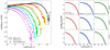 |
Fig. 1. Left: Dark matter HMF for the different simulations considered in this paper. The shaded regions show the measurements based on the MS (1σ Poissonian scatter); the dashed lines correspond to the MSII simulation; and the squares with errorbars are for the PMS simulation (1σ Poissonian scatter). Right: Impact of different cosmological parameters on the evolution of the HMF. The left-most panels show the HMFs expected for the MS and PMS cosmological models (dashed black and solid red lines, respectively). In the central and right-most panels, the HMFs for the MS are compared with runs with theoretical expectations obtained modifying the following parameters: σ8 (assumed to be the same as in the PMS; blue solid line); σ8 and the spectral index (as in the PMS; cyan dotted line); Ωm (as in the PMS; green solid line). |
2.2. GAEA
For this study we considered predictions from our latest rendition of the GAEA semi-analytic model (SAM). The approach starts from a statistical description of the assembly of the large-scale structure (i.e. a merger tree) that can be either analytically derived or extracted from numerical experiments. Galaxies are assumed to form within DM haloes, under the effect of a complex network of physical processes responsible for energy and mass exchanges among different baryonic components. SAMs follow the evolution of galaxy populations by numerically solving a system of differential equations, aiming at describing specific physical mechanisms, using parametrizations derived from empirical, numerical, or theoretical arguments. The parameters involved are calibrated against a well-defined set of observational constraints by efficiently sampling the parameter space. The main advantage of the SAM approach lies in its reduced computational demand with respect to hydrodynamical simulations: they are the optimal tool for studying galaxy evolution over large cosmological volumes, with enough flexibility to extensively test different physical models, explore their associated parameter space, and therefore the impact of individual physical mechanisms to set the observed properties of different galaxy populations.
GAEA builds from the model originally presented in De Lucia & Blaizot (2007), but now includes several improvements and further developments, in particular (a) the modelling of chemical enrichment, based on a non-instantaneous treatment of the ejection of gas, metals, and energy that accounts for the mass dependence of stellar lifetimes (De Lucia et al. 2014; b) an improved treatment for stellar feedback, partially based on results of high-resolution hydrodynamical simulations (Hirschmann et al. 2016); and (c) a detailed tracing of the evolution of angular momentum (Xie et al. 2017). The latest rendition of the model is presented in De Lucia et al. (2024, DL24 hereafter) and merges independently developed versions, namely (d) the Xie et al. (2017) explicit partition of the cold gas into its atomic and molecular components; (e) the Xie et al. (2020) treatment for the non-instantaneous stripping of cold and hot gas in satellites galaxies; and (f) the Fontanot et al. (2020) modelling for cold gas accretion onto SMBHs and the onset of AGN-driven outflows. This new version of the GAEA model has been calibrated on the z < 3 evolution of the GSMF, on the z < 4 evolution of the AGN-LF, and on the local HI and H2 mass function. DL24 shows that it correctly reproduces the evolution of the fraction and number densities of quenched galaxies up to z ∼ 4, providing the largest number densities of massive galaxies at z > 3 among similar theoretical models, predicting the rise of the first massive quenched galaxies at z ∼ 6 − 7 (Xie et al. 2024). A more throughout analysis of the properties of the highest-z galaxies, especially in terms of their predicted UV luminosities as seen by JWST, will be presented in forthcoming work (Cantarella et al., in prep.). We note that the latest GAEA rendition preserves the good agreement with a variety of observational constraints that have been explored in recent years, such as the evolution of the mass-metallicity relations (Fontanot et al. 2021, both for the gaseous and stellar phases – see also Fig. A.5), the z > 3 GSMF, and the cosmic star formation rate density up to the highest redshifts for which observations are available (Fontanot et al. 2017).
3. Convergence of model predictions on different simulations
In order to appreciate the effect of a change in the cosmological parameters and resolution on the predictions of our model, we consider GAEA runs over merger trees extracted from the PMS, MS, and MSII. All the predictions we discuss in the following sections are based on model realization using the same values for the relevant physical parameters involved in the SAM definition. These parameters have been calibrated on the MS trees and correspond to the model presented in DL24. We list the most relevant in Table 2. In the following, we show model predictions convolved with an estimated error on stellar and gaseous masses of 0.25 dex, thereby taking the Eddington bias (Jeffreys 1938; Eddington 1940) into account. The uncertainty considered represents a conservative choice, especially at high-z. We contrast the model predictions from the different simulations with compilations of observational data used in our previous works. In this section (Fig. 2) we focus on a basic set of physical properties, whose evolution is crucial for understanding the process of galaxy assembly, such as the GSMF (left panel) from z ∼ 0 to z ∼ 3 and the AGN-LF (right panel) from z ∼ 0 to z ∼ 4. These are among the main observables used to calibrate our model. In Appendix A we include additional observational constraintsconsidered for model calibration in addition to several predictions we consider in our recent work.
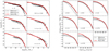 |
Fig. 2. Left: Redshift evolution of the galaxy stellar mass function, the data points correspond to the compilation used in Fontanot et al. (2009, see complete reference list for their Fig. 1). Right: Redshift evolution of the bolometric QSO/AGN-LF; the shaded regions show the expected space density from the empirical estimate of Shen et al. (2020). The black solid, black dashed, and red solid lines refer the GAEA model version presented in DL24 and run on the MS, MSII, and PMS simulations, respectively. |
It is remarkable that predictions corresponding to realizations run on different simulations show such a high level of consistency. This shows that our latest rendition of the GAEA model exhibits an improved convergence with respect to previous versions. This is remarkable for the predicted evolution of the AGN-LF: the space density of faint AGN is very sensitive to the number of trigger events (i.e. mergers) and in the past this has limited the convergence of our model to relatively bright luminosities (see e.g. Fig. A.2 in Fontanot et al. 2020). The latest GAEA version shows a good convergence between the MS and the PMS runs down to Lbolo ∼ 1042 erg/s at z < 1, and down to Lbolo ∼ 1044 erg/s at higher redshifts; predictions from the PMS and MSII agree even better around the knee of the LF, while at brighter luminosities, the MSII lacks the volume to correctly reproduce the rarer sources. For all other statistical estimators the level of convergence between the different runs is high, and in most cases predictions based on different simulations are virtually indistinguishable. We interpret this effect as a result of the interplay between the improved modelling of star formation, based on the partition of the cold gas as in Xie et al. (2017), and the new prescription for cold gas accretion onto the central SMBHs (Fontanot et al. 2020). Both physical mechanisms act as regulators of the total amount of cold gas available for star formation, chemical enrichment, and SMBH accretion. In fact, versions of the model implementing just one of the two physical mechanisms (and run on different simulations) do not achieve the same level of convergence over such a wide range of redshifts and physical properties as the model presented here.
4. Clustering analysis
4.1. Redshift evolution of the two-point correlation function
We then considered the predicted correlation functions for our model universes at different redshifts. In the following, we focus on the projected two-point correlation function w(rp); this choice makes the comparison with observational data straightforward, and does not have to rely on de-projection algorithms. We studied the evolution of the projected correlation function using estimates from several surveys. Going from low-z to higher redshifts, we compared against results from SDSS (Li et al. 2006, z ∼ 0.1, maximum integration scale2πmax = 40 h−1 Mpc), GAMA (Farrow et al. 2015, z < 0.2, πmax = 40 h−1 Mpc), VIPERS (Marulli et al. 2013, 0.5 < z < 1.1, πmax = 30 h−1 Mpc), DEEP2 (Li et al. 2006, z ∼ 0.9, πmax = 40 h−1 Mpc), VVDS (Meneux et al. 2008, z ∼ 0.9, πmax = 20 h−1 Mpc), zCOSMOS (zCOSMOS Meneux et al. 2009, z ∼ 0.9, πmax = 20 h−1 Mpc), and VUDS (Durkalec et al. 2018, z ∼ 2.7, πmax = 20 h−1 Mpc). We show all these observational measurements in Fig. 3 and contrast them with the prediction from GAEA realizations based on the MS (black dashed lines), the MSII (dotted lines), or the PMS (red solid lines). Where not visible, the dotted lines (MSII) overlap with the dashed lines (MSI). We do not show predictions from the MSII for bins corresponding to M⋆ > 1011 h−2 M⊙ as there are too few galaxies above this mass limit to provide a statistical estimate for the 2pCF. We computed w(rp) from GAEA using the Python CORRFUNC package (Sinha & Garrison 2020); model galaxy samples were extracted from the simulated volumes considering all galaxies in the stellar mass range indicated in the legend, i.e. we did not attempt to replicate selection criteria specific of the different surveys considered. In each plot (and in Figs. 4 and 6), the model estimates were computed using the same πmax as in the observed samples we used for comparison, except for the z ∼ 0.9 panel. In this case we show the model predictions corresponding to πmax = 40 h−1 Mpc (i.e. the value used in the DEEP2 survey). In our analysis we included an estimate for the typical uncertainty on M⋆ by convolving the intrinsic predictions of the model with a log-normal error distribution of amplitude 0.25 dex. We checked that our main conclusions do not depend on this choice as w(rp) predictions based on intrinsic M⋆ provide a consistent picture. We also explored the impact of uncertainties in the theoretical w(rp) determination by computing the jackknife errors using the COSMOBOLOGNALIB package (Marulli et al. 2016). We show these uncertainties for the PMS as the orange areas. We also assessed the impact of cosmic variance on the comparison between data and model predictions: we randomly extracted from the PMS 100 boxes with the same volume as the observational survey. The yellow areas in Fig. 3 highlight the range covered by these sub-volumes. Overall, the jackknife errors are relevant at large separations and for the most massive galaxies. Cosmic variance is relevant at the highest redshift considered and for small surveyed volumes, where it leads to errors that are slightly larger than those based on jackknife at intermediate scales.
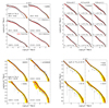 |
Fig. 3. Redshift evolution of the projected two-point correlation function at different bins of stellar mass (as labelled). Upper left: Data from SDSS at z ∼ 0 (Li et al. 2006). Upper right: Data from VIPERS at 0.5 < z < 1.1 (Marulli et al. 2013). Lower left: Data at z ∼ 0.9 from VVDS (Meneux et al. 2008), zCOSMOS (Meneux et al. 2009), DEEP2 obtained using the same techniques as in Li et al. (2006). Lower right: Data from VUDS at 2 < z < 3.5 (Durkalec et al. 2018). GAEA predictions refer to the realizations run on the MS (black dashed line) and on the PMS (red solid line) as in Fig. 2. The blue dot-dashed line refers to the 2pCF computed using the central galaxies belonging to DMHs in a mass range derived from the stellar mass range using the Behroozi et al. (2013) relation (see main text for details). The orange and yellow areas correspond to the jackknife estimated errors and cosmic variance dispersion, respectively. |
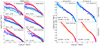 |
Fig. 4. Left: Projected two-point correlation function for red and blue galaxies at z ∼ 0.1; data from Li et al. (2006). Right: Projected two-point correlation function for star forming and quiescent galaxies; data from Coil et al. (2017). GAEA predictions refer to the realizations run on the MS (dashed lines) and on the PMS (solid lines) as in Fig. 2. |
Overall, the level of agreement between theoretical and observed correlation functions is satisfactory over the entire redshift range considered. Models run on the MS, MSII, and PMS agree well with each other, but for a slight tendency of the MS and MSII runs to predict systematically stronger correlations than PMS. The effect is more pronounced at low stellar masses and close separations, and we ascribe it to the larger value of σ8 used in the MS and MSII. At z < 0.2 (Fig. 3, upper left panel), the theoretical w(rp) are very close to the SDSS constraints for 109 < M⋆[h−2 M⊙]< 1011. Above and below this mass range, the model predictions respectively slightly underestimate and overestimate the measured clustering signal.
The lower normalization of the 2pCF for galaxies more massive than 1011 h−2 M⊙ is connected with the overprediction of the high-mass end of the z ∼ 0 GSMF (top left panel of Fig. 2). In this mass range, our model galaxies lie above the Mvir versus M⋆ relation that can be inferred from data using a classical sub-halo abundance matching technique (Behroozi et al. 2013; Moster et al. 2013), i.e. GAEA massive galaxies tend to live in DMHs less massive than can be inferred using halo occupation distribution statistics.
For galaxies in the 108.5 < M⋆[h−2 M⊙]< 109 mass bin, the overprediction of the clustering amplitude is a combination of different effects, all linked to the mass distribution of satellites and centrals in the smallest resolved DM haloes. In particular, at small scales (i.e. ≲2 h−1 Mpc) orphan galaxies (i.e. satellite galaxies whose sub-structure has fallen below the resolution limit of the simulation) represent a relevant population and their orbital evolution and merging times estimates might be incorrect (see e.g. De Lucia et al. 2010 for a discussion). There is a clear difference in the predictions at the smallest scales probed, due to the different number of orphan galaxies in the MS and MSII. At scales larger than 2 h−1 Mpc, the strongest clustering signal is connected with the mass distribution of satellite galaxies, as shown in Wang et al. (2013a), for example. These authors showed that in order to reproduce at the same time the GSMF and 2pCF in the framework of a halo occupation distribution model, satellite galaxies should be less massive than centrals, on average, at fixed stellar mass. They also considered the results from two independent semi-analytic models that struggled to reproduce these results, a problem that is shared by our GAEA model. The satellite stellar mass mismatch is connected to the uncertainties in the modelling of merging times, but also to the effect of assembly bias (as in SAMs low-mass galaxies show the strongest correlation with halo formation timescales; see again Wang et al. 2013a). It is worth noting that GAEA lacks an explicit treatment for tidal stripping of stars from satellite galaxies, a process that could move model predictions in the right direction and whose impact we plan to study in future work.
Similar conclusions hold at intermediate redshifts (0.5 < z < 0.9) for VIPERS (Fig. 3, upper right panel). The situation is slightly more complex at z ∼ 0.9, where different surveys suggest slightly different normalization for w(rp). This could be due to the different surveyed volume or to the presence of overdensities (as in the case of the zCOSMOS sample, Meneux et al. 2009). Nonetheless, GAEA predictions lie within the clustering measurements obtained from different surveys at z ∼ 0.9 (Fig. 3, lower left panel) and the agreement with data is acceptable to the smallest separations measured. The predicted evolution of the w(rp) normalization at z ≲ 1 is rather small; in most cases w(rp) can be closely approximated by a single power law over a wide separation scale; GAEA also captures the observed flattening of the relation at low-z for the smallest separations probed by the SDSS.
Moving to higher redshifts (2 < z < 3.5), a larger discrepancy in the w(rp) normalization can found with respect to the VUDS data (Fig. 3, lower right panel): GAEA predictions are still consistent with the observational measurements within the uncertainties, but tend to lie systematically above the data. The cosmic variance can also have a non-negligible impact here (the VUDS volume correspond to ∼1.75 × 10⁷ Mpc3, roughly 1/175 of the PMS). Overall, we can conclude that GAEA is able to satisfactorily reproduce the observed evolutionary trends of the correlation strength up to z ≲ 3.5. This represents a non-trivialsuccess for our latest GAEA model release.
4.2. Colour–SFR dependence of the two-point correlation function
As we discuss above, several authors (see e.g. Wang et al. 2013b) have pointed out that the clustering strength depends not only on M⋆, but also on the star formation activity of galaxy population, with red and quiescent galaxies being more clustered than their blue and star-forming counterparts with similar M⋆. In Fig. 4 we compare model predictions with SDSS data at z ∼ 0.1 (Li et al. 2006, πmax = 40 h−1 Mpc) and data up to z ∼ 1.0 (Coil et al. 2017, πmax = 40 h−1 Mpc) obtained combining the PRIsm MUlti-object Survey (PRIMUS, Coil et al. 2011) with DEEP2. At all redshifts, we consider model predictions corresponding to quiescent and star-forming sub-samples, using separation thresholds based on their specific SFR (sSFR = SFR/M⋆), for consistency with our previous work (DL24).
At z ∼ 0.1, model galaxies are classified using a sSFR = 10−11 yr−1 separation. This is formally different than the choice for SDSS galaxies, which have been split according to their g − r colour; however, we checked that using a classifications based on galaxy colours (e.g. Springel et al. 2018) does not qualitatively change our main results. Overall, GAEA realizations show a stronger clustering signal of red galaxies with respect to blue galaxies, in qualitative agreement with observations. In more detail, our models reproduce well the clustering strength for red galaxies over the entire mass range considered. This is particularly true for the PMS realization, while some residual overestimate of the clustering signal holds at the lowest masses and smallest scales. It is worth noting that this is the range of scales and stellar masses where our model samples are dominated by orphan galaxies (which are typically associated with low SFRs and red colours). The clustering strength of blue galaxies is also reasonably well reproduced for intermediate masses (i.e. in the 109.5 < M⋆/[h−1 M⊙]< 1011 range). Outside this range, the clustering of star-forming galaxies shows the same trends discussed for the global population, thus suggesting that this galaxy population is driving the tensions between predictions and data reported in Sect. 4.1 and Fig. 3. At higher redshifts we contrast clustering estimates from the PRIMUS and DEEP2 surveys with GAEA predictions by splitting model galaxies into quiescent and star-forming sub-samples, using the same (redshift-dependent) sSFR threshold employed in the data (Coil et al. 2017):
 (1)
(1)
The agreement between data and model predictions in the single mass bin available (10.5 < Log(M⋆[h−2 M⊙]) < 11) is very good, both for the red and blue populations.
The comparison presented in Fig. 4 indicates that the GAEA realizations reproduce qualitatively the relative clustering amplitude between the red and blue populations. In order tobetter highlight this, we consider in Fig. 5 the ratio of the clustering amplitudes of the red and blue populations at different redshifts for some of the available mass bins. Figure 5 shows that the GAEA predictions reproduce qualitatively the observed trends, with deviations due to the discrepancies discussed in relation to Fig. 4. The results presented in this section suggest that the treatment for the physical mechanisms responsible for quenching in GAEA not only correctly reproduces the overall assembly and evolution of the quenched galaxy population (DL24, Xie et al. 2024), but it is also broadly consistent with their expected distribution in the large-scale structure. Therefore, this analysis represents a further positive test suggesting that GAEA correctly captures the relative role of internal and environmental processes in shaping the galaxy properties in different environments.
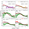 |
Fig. 5. Ratio of the projected two-point correlation function for red and blue galaxies. The data points have been arranged from Fig. 4. The green points refer to data from Li et al. (2006, SDSS at z ∼ 0.1); the diamonds and squares to data from Coil et al. (2017, PRIMUS+DEEP sample at z ∼ 0.5 and z ∼ 0.9). GAEA predictions refer to the realizations run on the MS (black dashed line) and on the PMS (red solid line), as in Fig. 2. |
4.3. Two-point correlation function for HI selected galaxies
In the previous sections, we discuss the 2pCF of galaxies selected on the basis of their stellar content. A complementary analysis involves the study of the cold gas content of galaxies, through the distribution of HI selected galaxies. The gas distribution in galaxies at low redshift can be mapped using the 21 cm HI hyper-fine emission line. In particular, the Arecibo Fast Legacy ALFA Survey (ALFALFA; Giovanelli et al. 2005) samples more than 5000 galaxies out to z ∼ 0.05, enabling the study of their clustering properties Papastergis et al. (2013), showed that HI selected galaxies exhibit a lower w(rp) amplitude with respect to stellar mass selected samples. Guo et al. (2017) used the 70% complete ALFALFA catalogue and showed that the 2pCF of of HI-selected galaxies depends strongly on the HI mass, i.e. galaxies with higher HI reservoirs are more strongly clustered on scales above a few megaparsecs than their counterparts with lower HI content. We compare Guo et al. (2017) estimates (πmax = 20 h−1 Mpc) at different HI-mass (MHI) thresholds with GAEA predictions in Fig. 6; we find a general agreement in the clustering amplitude and, more importantly, in its relative evolution as a function of MHI. The larger discrepancies are seen at the high-MHI end, although data and predictions are consistent within the statistical errorbars. This result is similar to those based on M⋆ selected galaxies, although the reference samples refer to different model galaxy populations as most massive galaxies at z ∼ 0 in GAEA have low gas fractions.
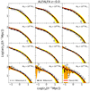 |
Fig. 6. Projected two-point correlation function for HI selected galaxies z ≲ 0.05; data from Guo et al. (2017). GAEA predictions refer to the realizations run on the MS (black dashed line) and on the PMS (red solid line), as in Fig. 2. |
5. Discussion and conclusions
In this paper we presented predictions of the latest version of the GAEA model, run on merger trees extracted from the PMS simulation. We compared model results against a compilation of observational measurements of galaxy clustering as a function of stellar mass and star formation rate, covering a wide redshift range from the local Universe up to the highest redshift when this measurement was possible (i.e. z ∼ 3.5). Our model shows a satisfactory agreement with the observed projected 2pCF, of comparable quality with respect to independent semi-analytic codes (L-GALAXIES, Guo et al. 2011; Henriques et al. 2017) and hydrodynamical simulations (Springel et al. 2018; Artale et al. 2017). At z ∼ 0, the GAEA results are close to those predicted from the TNG hydro-simulation suite (Springel et al. 2018). A quite good agreement with the data is found in the 109 < M⋆[h−2 M⊙]< 1011 stellar mass range and at the smallest scales, while the predicted 2pCT slightly underpredicts the observational measurements for the most massive galaxies. Similar results have also been found for the EAGLE simulation (Artale et al. 2017). Predictions from the L-GALAXIES model are closer to the observed w(rp) amplitude in the highest-mass bin, but they either overpredict (Guo et al. 2011) or underpredict (Henriques et al. 2017) the clustering of intermediate- to low-mass galaxies (i.e. 109 ≲ M⋆[h−2 M⊙]≲1010). At the lowest mass bin, our model predictions overpredict the clustering signal, similarly to what was found by Guo et al. (2011). Overall, our model does notpredict a significant evolution of the clustering strength with redshift, in good agreement with independent theoretical predictions (Artale et al. 2017) and observational measurements up to z ∼ 1 (Marulli et al. 2013). At higher redshift, the data seem to suggest a more significant evolution of the clustering amplitude than the model predictions, resulting in an overprediction with respect to the observed normalization of the 2pCF. Considering the observational uncertainties, the model predictions are still consistent with the observational data, and more data at z ≳ 2 are needed to clarify whether the highlighted discrepancy is significant.
Figure 7 shows the dependence of the clustering length r0 on galaxy stellar mass and its redshift evolution as predicted by our runs, and compares it to observational measurements. We computed r0 from the intrinsic three-dimensional 2pCF (ξ), directly computed from our model outputs, defined as the scale corresponding to ξ(r0) = 1. GAEA predicts a significant increase in r0 as a function of stellar mass. For M⋆ > 1010 h−2 M⊙ the predicted r0 values are in reasonable agreement with the observational constraints (see e.g. Foucaud et al. 2010; Wake et al. 2011; Lin et al. 2012; Marulli et al. 2013), with a clear excess of the predicted value of r0 for galaxy stellar masses below ∼1010 h−2 M⊙. At fixed stellar mass, we find only a weak evolution of r0 at z < 2, in agreement with the numerical results from Artale et al. (2017) and Springel et al. (2018). A significant discrepancy between the model predictions and data is found at z ≳ 2: GAEA predicts a factor of ∼2 increase in r0 at fixed stellar mass; the data exhibit a slower trend as a function of galaxy stellar mass evolution.
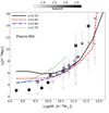 |
Fig. 7. Clustering length r0 as a function of stellar mass. The GAEA predictions for the PMS at different redshifts are marked by different colours and linetypes (see legend). The data compilation is from Meneux et al. (2008, triangles), Foucaud et al. (2010, stars), Wake et al. (2011, hexagons), Lin et al. (2012, squares), Marulli et al. (2013, diamonds), Durkalec et al. (2018, circles). |
If we split our model galaxies into star-forming and quiescent samples, we find that GAEA correctly reproduces the increased clustering of red quiescent galaxies with respect to blue star-forming systems. Overall, the red population shows a better agreement with the data over the entire galaxy mass range considered, while the blue galaxies exhibit both an excess of the clustering signal for low stellar masses (M⋆ < 109h−2 M⊙) and an underprediction of the 2pCF at high masses (M⋆ > 1011h−2 M⊙). Both discrepancies are consistent with the tensions we find between the model prediction and the data for the global population. In general, the GAEA results align well with similar comparisons shown in Guo et al. (2011) and Springel et al. (2018) for an independent semi-analytic and hydrodynamical model of galaxy formation. These models tend to better reproduce the properties of the star-forming population, while overpredicting the clustering of the red population at intermediate stellar mass (in particular, for M⋆ ∼ 109 − 1010h−2 M⊙).
Finally, we also compared our model predictions with clustering measurement for HI-selected galaxies in the ALFA survey, and we find a good agreement over the entire MHI mass range considered. Overall, the results discussed in this paper demonstrate that the proposed modelling of physical mechanisms responsible for gas consumption, recycling, and quenching in GAEA (both internal and environmental) are able to capture the main trends found for the observed clustering strength and its variation with stellar mass, SF activity and HI content. We note that our model has not been calibrated to reproduce galaxy clustering, which thus represents a genuine model prediction. This is not a trivial success, and it shows that our approach is able to recover not only the global properties of galaxy populations in a statistical sense, but also their spatial distribution in the LSS. The general good agreement between model predictions and data for the one-halo term (i.e. at scales ≲2−3 h−1 Mpc) for stellar masses down to M⋆ ∼ 109 h−2 M⊙, suggests that the satellite distribution within haloes is correctly reproduced, at least down to this stellar mass limit. This implies that our treatment for the evolution of satellite galaxies as in Xie et al. (2020) is generally effective in recovering the main properties of this population, both in terms of stellar mass and star formation activity. The excess of clustering signal found for lower stellar masses can be understood as a combination of different effects. On the one hand, satellite galaxies residing in low-mass haloes are more massive with respect to what is found in sub-halo abundance matching models constrained to reproduce both the 2pCF and the GSMF (Wang et al. 2013a). The clustering signal excess for the two-halo term (i.e. at scales ≳2−3 h−1 Mpc) suggests that GAEA is predicting a larger than expected number of satellites in corresponding haloes and this can be related to our treatment of the merging times for orphan galaxies.
In summary, the latest GAEA version shows a remarkable level of agreement for model predictions run on merger trees extracted from simulations of different resolution and (slightly) different ΛCDM cosmological parameters. This result is driven by the interplay between the new treatment for AGN (and its feedback on the host galaxies) and the explicit partitioning of cold gas into its atomic and molecular components. Both physical mechanisms act as regulators of the cold gas in model galaxies. GAEA reasonably reproduces the observed dependence of galaxy clustering on stellar mass and star formation activity. Moreover, the model predictions are also broadly consistent with the clustering measurements corresponding to HI-selected galaxies. This is an important confirmation that our treatment of the mechanisms acting on the baryonic component of galaxies, and satellites in particular, is able to capture the relevant physical dependences. GAEA predicts a small redshift evolution of the amplitude of the 2pCF: this is consistent with the available data up to z ∼ 3.5, which we interpret as another indication that our model is able to correctly connect galaxies with their environment. At higher redshifts, our model tends to underpredict the observational measurements. However, larger observational samples are needed to draw firmer conclusions in this redshift regime.
Visible Multi Object Spectrograph.
The maximum integration scale πmax represents the finite upper limit used for the integration of the real-space correlation function.
Acknowledgments
An introduction to GAEA, a list of our recent work, as well as a data file containing published model predictions, can be found at https://sites.google.com/inaf.it/gaea/home. We acknowledge the use of INAF-OATs computational resources within the framework of the CHIPP project (Taffoni et al. 2020) and the INAF PLEIADI program (https://www.ict.inaf.it/computing/pleiadi/). This work used the DiRAC@Durham facility managed by the Institute for Computational Cosmology on behalf of the STFC DiRAC HPC Facility (www.dirac.ac.uk). The equipment was funded by BEIS capital funding via STFC capital grants ST/P002293/1, ST/R002371/1 and ST/S002502/1, Durham University and STFC operations grant ST/R000832/1. DiRAC is part of the National e-Infrastructure. We thank the anonymous referee for a careful reading of the manuscript that helped us improve the quality of the presentation of our results. We thank Cheng Li for sharing his observational estimates for the clustering signal in the SDSS and DEEP2 surveys. We acknowledge stimulating discussions with Andrea Biviano, Alessandra Fumagalli, Federico Marulli, Pierluigi Monaco and Emiliano Sefusatti. MH acknowledges funding from the Swiss National Science Foundation (SNSF) via a PRIMA grant PR00P2-193577 ‘From cosmic dawn to high noon: the role of BHs for young galaxies’.
References
- Artale, M. C., Pedrosa, S. E., Trayford, J. W., et al. 2017, MNRAS, 470, 1771 [NASA ADS] [CrossRef] [Google Scholar]
- Baugh, C. M., Gonzalez-Perez, V., Lagos, C. D. P., et al. 2019, MNRAS, 483, 4922 [NASA ADS] [CrossRef] [Google Scholar]
- Behroozi, P. S., Wechsler, R. H., & Conroy, C. 2013, ApJ, 770, 57 [NASA ADS] [CrossRef] [Google Scholar]
- Boylan-Kolchin, M., Springel, V., White, S. D. M., Jenkins, A., & Lemson, G. 2009, MNRAS, 398, 1150 [Google Scholar]
- Coil, A. L., Newman, J. A., Cooper, M. C., et al. 2006, ApJ, 644, 671 [NASA ADS] [CrossRef] [Google Scholar]
- Coil, A. L., Blanton, M. R., Burles, S. M., et al. 2011, ApJ, 741, 8 [Google Scholar]
- Coil, A. L., Mendez, A. J., Eisenstein, D. J., & Moustakas, J. 2017, ApJ, 838, 87 [Google Scholar]
- Cole, S., & Kaiser, N. 1989, MNRAS, 237, 1127 [NASA ADS] [Google Scholar]
- Cooray, A., & Sheth, R. 2002, Phys. Rep., 372, 1 [Google Scholar]
- Davis, M., & Geller, M. J. 1976, ApJ, 208, 13 [NASA ADS] [CrossRef] [Google Scholar]
- De Lucia, G., & Blaizot, J. 2007, MNRAS, 375, 2 [Google Scholar]
- De Lucia, G., Boylan-Kolchin, M., Benson, A. J., Fontanot, F., & Monaco, P. 2010, MNRAS, 406, 1533 [NASA ADS] [Google Scholar]
- De Lucia, G., Tornatore, L., Frenk, C. S., et al. 2014, MNRAS, 445, 970 [Google Scholar]
- De Lucia, G., Fontanot, F., Xie, L., & Hirschmann, M. 2024, A&A, 687, A68 [NASA ADS] [CrossRef] [EDP Sciences] [Google Scholar]
- Durkalec, A., Le Fèvre, O., Pollo, A., et al. 2018, A&A, 612, A42 [NASA ADS] [CrossRef] [EDP Sciences] [Google Scholar]
- Eddington, A. S. 1940, MNRAS, 100, 354 [Google Scholar]
- Farrow, D. J., Cole, S., Norberg, P., et al. 2015, MNRAS, 454, 2120 [Google Scholar]
- Fletcher, T. J., Saintonge, A., Soares, P. S., & Pontzen, A. 2021, MNRAS, 501, 411 [Google Scholar]
- Fontanot, F., De Lucia, G., Monaco, P., Somerville, R. S., & Santini, P. 2009, MNRAS, 397, 1776 [NASA ADS] [CrossRef] [Google Scholar]
- Fontanot, F., Hirschmann, M., & De Lucia, G. 2017, ApJ, 842, L14 [Google Scholar]
- Fontanot, F., De Lucia, G., Hirschmann, M., et al. 2020, MNRAS, 496, 3943 [CrossRef] [Google Scholar]
- Fontanot, F., Calabrò, A., Talia, M., et al. 2021, MNRAS, 504, 4481 [CrossRef] [Google Scholar]
- Foucaud, S., Conselice, C. J., Hartley, W. G., et al. 2010, MNRAS, 406, 147 [Google Scholar]
- Giovanelli, R., Haynes, M. P., Kent, B. R., et al. 2005, AJ, 130, 2598 [Google Scholar]
- Guo, Q., White, S., Boylan-Kolchin, M., et al. 2011, MNRAS, 413, 101 [Google Scholar]
- Guo, H., Li, C., Zheng, Z., et al. 2017, ApJ, 846, 61 [NASA ADS] [CrossRef] [Google Scholar]
- Haynes, M. P., Giovanelli, R., Martin, A. M., et al. 2011, AJ, 142, 170 [Google Scholar]
- Henriques, B. M. B., White, S. D. M., Thomas, P. A., et al. 2017, MNRAS, 469, 2626 [Google Scholar]
- Hirschmann, M., De Lucia, G., & Fontanot, F. 2016, MNRAS, 461, 1760 [Google Scholar]
- Jeffreys, H. 1938, MNRAS, 98, 190 [Google Scholar]
- Jenkins, A. 2013, MNRAS, 434, 2094 [NASA ADS] [CrossRef] [Google Scholar]
- Jenkins, A., Frenk, C. S., Pearce, F. R., et al. 1998, ApJ, 499, 20 [Google Scholar]
- Jones, M. G., Haynes, M. P., Giovanelli, R., & Moorman, C. 2018, MNRAS, 477, 2 [Google Scholar]
- Keres, D., Yun, M. S., & Young, J. S. 2003, ApJ, 582, 659 [NASA ADS] [CrossRef] [Google Scholar]
- Kormendy, J., & Ho, L. C. 2013, ARA&A, 51, 511 [Google Scholar]
- Li, C., Kauffmann, G., Jing, Y. P., et al. 2006, MNRAS, 368, 21 [NASA ADS] [CrossRef] [Google Scholar]
- Lin, L., Dickinson, M., Jian, H.-Y., et al. 2012, ApJ, 756, 71 [NASA ADS] [CrossRef] [Google Scholar]
- Marulli, F., Bolzonella, M., Branchini, E., et al. 2013, A&A, 557, A17 [NASA ADS] [CrossRef] [EDP Sciences] [Google Scholar]
- Marulli, F., Veropalumbo, A., & Moresco, M. 2016, Astron. Comput., 14, 35 [Google Scholar]
- McConnell, N. J., & Ma, C.-P. 2013, ApJ, 764, 184 [Google Scholar]
- Meneux, B., Guzzo, L., Garilli, B., et al. 2008, A&A, 478, 299 [NASA ADS] [CrossRef] [EDP Sciences] [Google Scholar]
- Meneux, B., Guzzo, L., de la Torre, S., et al. 2009, A&A, 505, 463 [NASA ADS] [CrossRef] [EDP Sciences] [Google Scholar]
- Mostek, N., Coil, A. L., Cooper, M., et al. 2013, ApJ, 767, 89 [NASA ADS] [CrossRef] [Google Scholar]
- Moster, B. P., Naab, T., & White, S. D. M. 2013, MNRAS, 428, 3121 [Google Scholar]
- Murray, S. G., Power, C., & Robotham, A. S. G. 2013, Astron. Comput., 3, 23 [CrossRef] [Google Scholar]
- Papastergis, E., Giovanelli, R., Haynes, M. P., Rodríguez-Puebla, A., & Jones, M. G. 2013, ApJ, 776, 43 [Google Scholar]
- Planck Collaboration XVI. 2014, A&A, 571, A16 [NASA ADS] [CrossRef] [EDP Sciences] [Google Scholar]
- Pollo, A., Guzzo, L., Le Fèvre, O., et al. 2006, A&A, 451, 409 [NASA ADS] [CrossRef] [EDP Sciences] [Google Scholar]
- Sánchez, A. G., Baugh, C. M., Percival, W. J., et al. 2006, MNRAS, 366, 189 [Google Scholar]
- Shen, X., Hopkins, P. F., Faucher-Giguère, C.-A., et al. 2020, MNRAS, 495, 3252 [Google Scholar]
- Sinha, M., & Garrison, L. H. 2020, MNRAS, 491, 3022 [Google Scholar]
- Skibba, R. A., Smith, M. S. M., Coil, A. L., et al. 2014, ApJ, 784, 128 [NASA ADS] [CrossRef] [Google Scholar]
- Spergel, D. N., Verde, L., Peiris, H. V., et al. 2003, ApJS, 148, 175 [Google Scholar]
- Springel, V., White, S. D. M., Tormen, G., & Kauffmann, G. 2001, MNRAS, 328, 726 [Google Scholar]
- Springel, V., White, S. D. M., Jenkins, A., et al. 2005, Nature, 435, 629 [Google Scholar]
- Springel, V., Pakmor, R., Pillepich, A., et al. 2018, MNRAS, 475, 676 [Google Scholar]
- Taffoni, G., Becciani, U., Garilli, B., et al. 2020, ArXiv e-prints [arXiv:2002.01283] [Google Scholar]
- Tinker, J., Kravtsov, A. V., Klypin, A., et al. 2008, ApJ, 688, 709 [Google Scholar]
- Wake, D. A., Whitaker, K. E., Labbé, I., et al. 2011, ApJ, 728, 46 [NASA ADS] [CrossRef] [Google Scholar]
- Wang, L., De Lucia, G., & Weinmann, S. M. 2013a, MNRAS, 431, 600 [Google Scholar]
- Wang, L., Weinmann, S. M., De Lucia, G., & Yang, X. 2013b, MNRAS, 433, 515 [NASA ADS] [CrossRef] [Google Scholar]
- Xie, L., De Lucia, G., Hirschmann, M., Fontanot, F., & Zoldan, A. 2017, MNRAS, 469, 968 [Google Scholar]
- Xie, L., De Lucia, G., Hirschmann, M., & Fontanot, F. 2020, MNRAS, 498, 4327 [NASA ADS] [CrossRef] [Google Scholar]
- Xie, L., De Lucia, G., Fontanot, F., et al. 2024, ApJ, 966, L2 [NASA ADS] [CrossRef] [Google Scholar]
- Zehavi, I., Blanton, M. R., Frieman, J. A., et al. 2002, ApJ, 571, 172 [NASA ADS] [CrossRef] [Google Scholar]
- Zwaan, M. A., Meyer, M. J., Staveley-Smith, L., & Webster, R. L. 2005, MNRAS, 359, L30 [NASA ADS] [CrossRef] [Google Scholar]
Appendix A: Additional model predictions
In this Appendix we show additional observational constraints to further explore the convergence of the latest GAEA model, and to demonstrate that our previously published results hold in the latest rendition of our model. We consider in Fig. A.1 the z∼0 distribution of sSFR in stellar mass bins and in Fig. A.2 the evolution of the main sequence of star-forming galaxies. In the latter figure, model star-forming galaxies have been selected as those with sSFR larger than 0.3/tH, where tH is the Hubble time at the redshift under consideration. Figure A.3 shows the z∼0 scaling relation between the mass of the central SMBH (MBH) and the mass of the spheroidal component (MBulge), while Fig. A.4 shows the gas-phase and stellar mass-metallicity relations. In Fig. A.5, we report the mass functions at z = 0 for the neutral and molecular gas components. These distributions have been used for the calibration of the model on MS merger trees (Xie et al. 2017; De Lucia et al. 2024). Figure A.5 shows that for the HI and H2 mass function the consistency between the model realizations run on different simulations is higher (i.e. it extends to smaller gas masses) than previous versions of the model (see e.g. Fig. 7 in Xie et al. 2017).
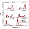 |
Fig. A.1. Specific star formation rate distribution in stellar mass bins, compared to SDSS DR8 observational estimates (grey shaded histograms). The MS and MSII histograms have been slightly shifted (by 0.05 dex) for clarity. The black solid, black dashed, and red solid lines refer the GAEA model version presented in DL24 and run on MS, MSII, and PMS, respectively. |
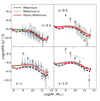 |
Fig. A.2. Redshift evolution of the main sequence of star-forming galaxies. The line types and colours are as in Fig. A.1; the data points correspond to the compilations used in Fontanot et al. (2009, filled symbols, see complete reference list for their Fig. 5) and in Xie et al. (2017, empty symbols, see complete reference list for their Fig. 11). |
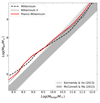 |
Fig. A.3. MBH-MBulge scaling relation at z∼0. The shaded areas correspond to the best fit relations of Kormendy & Ho (2013) and McConnell & Ma (2013); for both relations we assume a scatter of 0.3 dex. The line types and colours are as in Fig. A.1. |
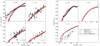 |
Fig. A.4. Left: Redshift evolution of the cold gas metallicity as a function of stellar mass (following Fontanot et al. 2021, we apply a downwards 0.1 dex shift to the intrinsic predictions). Right: Stellar mass-metallicity relation at different redshifts. The line types and colours are as in Fig. A.1. In both panels the data points correspond to the compilation used in Fontanot et al. (2021, see complete reference list for their Fig. 1). |
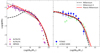 |
Fig. A.5. HI and H2 mass functions at z∼0 (left and right panel respectively). The observational data are from Keres et al. (2003, blue empty diamonds), Zwaan et al. (2005, purple stars), Haynes et al. (2011, magenta triangles), Jones et al. (2018, pink empty circles), and Fletcher et al. (2021, light green hexagons). The line types and colours are as in Fig. A.1. The model predictions have been convolved with an estimated 0.25 dex error on the gas mass determination. |
All Tables
Numerical and cosmological parameters for the simulations considered in this work.
All Figures
|
Fig. 1. Left: Dark matter HMF for the different simulations considered in this paper. The shaded regions show the measurements based on the MS (1σ Poissonian scatter); the dashed lines correspond to the MSII simulation; and the squares with errorbars are for the PMS simulation (1σ Poissonian scatter). Right: Impact of different cosmological parameters on the evolution of the HMF. The left-most panels show the HMFs expected for the MS and PMS cosmological models (dashed black and solid red lines, respectively). In the central and right-most panels, the HMFs for the MS are compared with runs with theoretical expectations obtained modifying the following parameters: σ8 (assumed to be the same as in the PMS; blue solid line); σ8 and the spectral index (as in the PMS; cyan dotted line); Ωm (as in the PMS; green solid line). |
| In the text | |
|
Fig. 2. Left: Redshift evolution of the galaxy stellar mass function, the data points correspond to the compilation used in Fontanot et al. (2009, see complete reference list for their Fig. 1). Right: Redshift evolution of the bolometric QSO/AGN-LF; the shaded regions show the expected space density from the empirical estimate of Shen et al. (2020). The black solid, black dashed, and red solid lines refer the GAEA model version presented in DL24 and run on the MS, MSII, and PMS simulations, respectively. |
| In the text | |
|
Fig. 3. Redshift evolution of the projected two-point correlation function at different bins of stellar mass (as labelled). Upper left: Data from SDSS at z ∼ 0 (Li et al. 2006). Upper right: Data from VIPERS at 0.5 < z < 1.1 (Marulli et al. 2013). Lower left: Data at z ∼ 0.9 from VVDS (Meneux et al. 2008), zCOSMOS (Meneux et al. 2009), DEEP2 obtained using the same techniques as in Li et al. (2006). Lower right: Data from VUDS at 2 < z < 3.5 (Durkalec et al. 2018). GAEA predictions refer to the realizations run on the MS (black dashed line) and on the PMS (red solid line) as in Fig. 2. The blue dot-dashed line refers to the 2pCF computed using the central galaxies belonging to DMHs in a mass range derived from the stellar mass range using the Behroozi et al. (2013) relation (see main text for details). The orange and yellow areas correspond to the jackknife estimated errors and cosmic variance dispersion, respectively. |
| In the text | |
|
Fig. 4. Left: Projected two-point correlation function for red and blue galaxies at z ∼ 0.1; data from Li et al. (2006). Right: Projected two-point correlation function for star forming and quiescent galaxies; data from Coil et al. (2017). GAEA predictions refer to the realizations run on the MS (dashed lines) and on the PMS (solid lines) as in Fig. 2. |
| In the text | |
|
Fig. 5. Ratio of the projected two-point correlation function for red and blue galaxies. The data points have been arranged from Fig. 4. The green points refer to data from Li et al. (2006, SDSS at z ∼ 0.1); the diamonds and squares to data from Coil et al. (2017, PRIMUS+DEEP sample at z ∼ 0.5 and z ∼ 0.9). GAEA predictions refer to the realizations run on the MS (black dashed line) and on the PMS (red solid line), as in Fig. 2. |
| In the text | |
|
Fig. 6. Projected two-point correlation function for HI selected galaxies z ≲ 0.05; data from Guo et al. (2017). GAEA predictions refer to the realizations run on the MS (black dashed line) and on the PMS (red solid line), as in Fig. 2. |
| In the text | |
|
Fig. 7. Clustering length r0 as a function of stellar mass. The GAEA predictions for the PMS at different redshifts are marked by different colours and linetypes (see legend). The data compilation is from Meneux et al. (2008, triangles), Foucaud et al. (2010, stars), Wake et al. (2011, hexagons), Lin et al. (2012, squares), Marulli et al. (2013, diamonds), Durkalec et al. (2018, circles). |
| In the text | |
|
Fig. A.1. Specific star formation rate distribution in stellar mass bins, compared to SDSS DR8 observational estimates (grey shaded histograms). The MS and MSII histograms have been slightly shifted (by 0.05 dex) for clarity. The black solid, black dashed, and red solid lines refer the GAEA model version presented in DL24 and run on MS, MSII, and PMS, respectively. |
| In the text | |
|
Fig. A.2. Redshift evolution of the main sequence of star-forming galaxies. The line types and colours are as in Fig. A.1; the data points correspond to the compilations used in Fontanot et al. (2009, filled symbols, see complete reference list for their Fig. 5) and in Xie et al. (2017, empty symbols, see complete reference list for their Fig. 11). |
| In the text | |
|
Fig. A.3. MBH-MBulge scaling relation at z∼0. The shaded areas correspond to the best fit relations of Kormendy & Ho (2013) and McConnell & Ma (2013); for both relations we assume a scatter of 0.3 dex. The line types and colours are as in Fig. A.1. |
| In the text | |
|
Fig. A.4. Left: Redshift evolution of the cold gas metallicity as a function of stellar mass (following Fontanot et al. 2021, we apply a downwards 0.1 dex shift to the intrinsic predictions). Right: Stellar mass-metallicity relation at different redshifts. The line types and colours are as in Fig. A.1. In both panels the data points correspond to the compilation used in Fontanot et al. (2021, see complete reference list for their Fig. 1). |
| In the text | |
|
Fig. A.5. HI and H2 mass functions at z∼0 (left and right panel respectively). The observational data are from Keres et al. (2003, blue empty diamonds), Zwaan et al. (2005, purple stars), Haynes et al. (2011, magenta triangles), Jones et al. (2018, pink empty circles), and Fletcher et al. (2021, light green hexagons). The line types and colours are as in Fig. A.1. The model predictions have been convolved with an estimated 0.25 dex error on the gas mass determination. |
| In the text | |
Current usage metrics show cumulative count of Article Views (full-text article views including HTML views, PDF and ePub downloads, according to the available data) and Abstracts Views on Vision4Press platform.
Data correspond to usage on the plateform after 2015. The current usage metrics is available 48-96 hours after online publication and is updated daily on week days.
Initial download of the metrics may take a while.