| Issue |
A&A
Volume 686, June 2024
|
|
|---|---|---|
| Article Number | A302 | |
| Number of page(s) | 13 | |
| Section | Extragalactic astronomy | |
| DOI | https://doi.org/10.1051/0004-6361/202348688 | |
| Published online | 21 June 2024 | |
Variation of the stellar initial mass function in semi-analytical models
III. Testing the cosmic-ray regulated integrated galaxy-wide initial mass function
1
INAF – Astronomical Observatory of Trieste, Via G. B. Tiepolo 11, 34143 Trieste, Italy
e-mail: This email address is being protected from spambots. You need JavaScript enabled to view it.
2
IFPU – Institute for Fundamental Physics of the Universe, Via Beirut 2, 34151 Trieste, Italy
3
INAF – Astronomical Observatory of Capodimonte, Sal. Moiariello, 16, 80131 Napoli, Italy
4
Astronomy Sector, Department of Physics, University of Trieste, Via Tiepolo 11, 34143 Trieste, Italy
5
Tianjin Astrophysics Center, Tianjin Normal University, Binshuixidao 393, 300384 Tianjin, PR China
6
Institute for Physics, Laboratory for Galaxy Evolution, EPFL, Observatoire de Sauverny, Chemin Pegasi 51, 1290 Versoix, Switzerland
7
Instituto de Radioastronomía y Astrofísica, UNAM, Campus Morelia, CP 58089 Morelia, Mexico
8
Sorbonne Université, CNRS, UMR 7095, Institut d’Astrophysique de Paris, 98 bis bd Arago, 75014 Paris, France
9
Instituto de Astrofísica de Canarias, 38200 La Laguna, Tenerife, Spain
10
Departamento de Astrofísica, Universidad de La Laguna, 38205 La Laguna, Tenerife, Spain
Received:
21
November
2023
Accepted:
15
April
2024
Abstract
Context. In our previous work, we derived the CR-IGIMF, which is a new scenario for a variable stellar initial mass function (IMF) that combines numerical results on the role played by cosmic rays (CR) in setting the thermal state of star-forming gas with the analytical approach of the integrated galaxy-wide IMF (IGIMF).
Aims. In this work, we study the implications of this scenario for the properties of local early-type galaxies (ETG) as inferred from dynamical, photometric, and spectroscopic studies.
Methods. We implemented a library of CR-IGIMF shapes in the framework of the galaxy evolution and assembly (GAEA) model. GAEA provides predictions for the physical and photometric properties of model galaxies and for their chemical composition. Our realization includes a self-consistent derivation of the synthetic spectral energy distribution for each model galaxy, which allows a direct derivation of the mass fraction in the mean IMF of low-mass stars (i.e., the dwarf-to-giant ratio, fdg) and a comparison with IMF-sensitive spectral features.
Results. The predictions of the GAEA model implementing the CR-IGIMF confirm our previous findings: It correctly reproduces both the observed excess of z ∼ 0 dynamical mass (mass-to-light ratio) with respect to spectroscopic (photometric) estimates assuming a universal MW-like IMF, and the observed increase in [α/Fe] ratios with stellar mass in spheroidal galaxies. Moreover, this realization reproduces the increasing trends of fdg and IMF-sensitive line strengths with velocity dispersion, although the predicted relations are significantly shallower than the observed ones.
Conclusions. Our results show that the CR-IGIMF is a promising scenario that reproduces at the same time dynamical, photometric, and spectroscopic indications of a varying IMF in local ETGs. The shallow relations found for spectral indices suggest that either a stronger variability as a function of galaxy properties or additional dependences (e.g., as a function of star forming gas metallicity) might be required to match the strength of the observed trends.
Key words: galaxies: abundances / galaxies: evolution / galaxies: formation / galaxies: fundamental parameters / galaxies: stellar content
© The Authors 2024
 Open Access article, published by EDP Sciences, under the terms of the Creative Commons Attribution License (https://creativecommons.org/licenses/by/4.0), which permits unrestricted use, distribution, and reproduction in any medium, provided the original work is properly cited.
This article is published in open access under the Subscribe to Open model. This email address is being protected from spambots. You need JavaScript enabled to view it. to support open access publication.
1. Introduction
The stellar initial mass function (IMF) is a fundamental ingredient in theoretical models of galaxy formation and evolution. For each given star formation episode, this statistical function defines the number of stars that formed per stellar mass bin. It therefore determines the number of SNe and the fraction of baryonic mass locked in long-living stars. Direct observations of star-forming regions in the Milky Way (MW) show a remarkable consistency in the derived shape of the IMF. Different authors proposed different functional shapes for the IMF in our galaxy (Salpeter 1955; Kroupa 2001; Chabrier 2003) that mainly differ in the very uncertainty regime of brown dwarfs, that is, at the low-mass end. Because the MW is the only galaxy in which we can currently measure the IMF using direct stellar counts, the near invariance of the results prompted the idea that it might be universal. However, from a theoretical perspective, the physical description of gravitational collapse and fragmentation of molecular clouds (MCs) is still debated in the literature (see, e.g., Krumholz 2014): Several models (Klessen et al. 2005; Weidner & Kroupa 2005; Hennebelle & Chabrier 2008; Papadopoulos et al. 2011; Narayanan & Davé 2013, among others) explored the range of possible IMF shapes depending on the physical properties of the interstellar medium (ISM).
A first indication that the IMF can indeed vary in environments different from those of the MW disc was reported by Klessen et al. (2007), who showed that the densest regions of the MW bulge (where stellar counts are still accessible) are better described by a different IMF (i.e., with a larger fraction of massive stars) than the IMF that applies to star-forming regions in the disc. Nonetheless, the assumption of a universal IMF is still used in almost all extragalactic studies. The main limitation for the study of the IMF shape over a variety of environments is our inability to resolve individual star clusters in external galaxies. Therefore, the only information currently accessible comes from the integrated light from composite stellar populations, which binds our ability to detect signatures of deviations from a universal IMF to indirect evidence. In the following we will consider as a reference universal IMF a Kroupa/Chabrier IMF, that is, a multislope broken power law, with a steeper high-mass end and a break at around 1 M⊙.
The evidence in favor of a varying IMF has steadily increased in recent times. Using galaxies from the GAMA1 survey, Gunawardhana et al. (2011) show that their optical colors and Hα line strengths suggest a flatter high-mass slope of the IMF at increasing Star Formation Rate (SFR). Dynamical studies in a sample of early-type galaxies (ETGs) in the ATLAS3D survey have revealed a systematic excess of dynamical mass-to-light ratios with respect to the expectations for a universal MW-like IMF based on observed photometry. This mass excess, α, increases with increasing galaxy velocity dispersion σ (Cappellari et al. 2012). A number of spectral features in the spectra of ETGs (e.g., NaI, TiO1 and TiO2) that are sensitive to temperature and/or surface gravity have been proposed as tracers of the ratio of low-mass and giant stars, and therefore, of the shape of the IMF from which they are formed. Several groups (see Conroy & van Dokkum 2012; Ferreras et al. 2013; La Barbera et al. 2013; Spiniello et al. 2014, among the others) have adopted this approach to conclude that the IMF slope at the low-mass end becomes steeper at increasing σ and/or stellar mass M⋆.
The main problem in interpreting this wealth of information in a consistent picture lies in our lack of physical understanding how the IMF shape varies as a function of the physical conditions of star-forming regions. IMFs with more low-mass or high-mass stars than the MW-like IMF are defined as bottom-heavy (or top-light) and top-heavy (or bottom-light), respectively. Spectroscopic studies seem to prefer a bottom-heavy solution for more massive galaxies (i.e., an IMF slope at the low-mass end that is steeper than the MW-like IMF). However, these studies were only based on the light of evolved stars, and therefore, this approach cannot provide any constraint on the high-mass end of the IMF. In principle, the dynamical technique is sensitive to the overall shape of the IMF, but it cannot distinguish between a bottom-heavy and a top-heavy scenario (Tortora et al. 2013). The observed α excess in the mass-to-light ratio can be interpreted either as a larger fraction of low-mass stars (giving rise to direct mass excess) or as a larger fraction of massive short-lived stars (giving rise to a decrease in the total light at late times).
The situation is further complicated by the detection of radial IMF gradients in ETGs (Martín-Navarro et al. 2015; La Barbera et al. 2017, 2021; van Dokkum et al. 2017; Sarzi et al. 2018). The results suggest that the low-mass end of the IMF becomes steeper toward the inner galaxy regions, but is comparable with an MW-like IMF in the outer regions. However, the same galaxies are more α-enriched in the inner regions than in the outskirts, and these [α/Fe] gradients may be better explained by a larger number of Type II SNe in the center (which suggests that the IMF becomes more top-heavy in the central regions). A possible solution to these tensions in the interpretation of the available data may be a time-varying IMF, where the two ends are allowed to vary independently over different timescales (see, e.g., Weidner et al. 2013; Ferreras et al. 2015). The fact that the two slopes can evolve in different directions at the same time makes it difficult to recast the differences with respect to the MW-like IMF into the standard definition of bottom-heavy or top-heavy IMF. In the following, we use this nomenclature only when discussing predictions related to one of the ends.
Galaxy formation models that self-consistently follow the interplay between IMF and galaxy properties represent a key tool for assessing the complexities in the interpretation of the photometric and spectroscopic data. In our previous work on the variable IMF hypothesis, we tested two different models, namely the integrated galaxy-wide IMF (IGIMF) by Weidner & Kroupa (2005) and the cosmic-ray- (CR) regulated IMF from Papadopoulos et al. (2011, PP11 hereafter). In brief, the former approach estimates the galaxy-wide IMF starting from a limited number of physically and observationally motivated axioms that can be recast as a function of the galaxy SFR. Instead, PP11 provided numerical estimates for the characteristic Jeans mass of young stars ( ) that form in a molecular cloud (MC) embedded in a CR energy density field of a given intensity. As energetic CRs can penetrate deeper into the core of these MCs, they can change the chemical and thermal state of the star-forming gas, thus affecting the emerging IMF. In this case, the dependence can be recast as a function of the SFR surface density2. In Fontanot et al. (2017a, F17) and Fontanot et al. (2018a, F18a), we presented theoretical models implementing the IGIMF and PP11 approaches, respectively, and discussed their implications for galaxy formation and evolution. These models are able to reproduce both the [α/Fe] versus stellar mass relation and the α excess of model ETGs at z ∼ 0. Nonetheless, the typical IMF variations in both these models mainly affect the slope of the high-mass end alone, while the low-mass end of the IMF is constant by construction. Therefore, these models are not able to reproduce the variation in the low-mass end slope derived from the spectroscopic studies of nearby ETGs.
In order to overcome this limitation, Fontanot et al. (2018b, F18b hereafter) proposed a new IMF derivation (dubbed CR-IGIMF), based on a combination of the two previous approaches. The main feature of the CR-IGIMF is the predicted evolution of both the high-mass and low-mass ends of the IMF as a function of the physical properties of the model galaxies. In F18b, we presented a preliminary analysis of the impact of this scenario on the spectral properties of the galaxies based on the idealized star formation histories that we used to estimate the mean IMF shapes of galaxies at z ∼ 0 as a function of their stellar mass. We concluded that the CR-IGIMF reproduces the observed trends qualitatively. The aim of this work is to explore the impact of this new IMF model on galaxy evolution in a more quantitative way, and in particular, to explore the constraints on the dynamical and spectroscopic properties of ETGs at z ∼ 0. To this end, we implemented the CR-IGIMF scenario in the framework of the semi-analytic model for galaxy evolution and assembly (GAEA) and employed the synthetic stellar population models of Vazdekis et al. (2012) to compute synthetic spectra of model galaxies. These implementations provide a new self-consistently calibrated tool to fully describe the IMF evolution during the star formation and assembly history of the model galaxies.
This paper is organized as follows. In Sect. 2, we lay out the theoretical framework of the CR-IGIMF derivation as presented in F18b. In Sect. 3, we introduce the implementation of the CR-IGIMF in the GAEA model. We present our main results and discuss them in the context of galaxy formation and evolution in Sect. 4. Finally, we outline our main conclusions in Sect. 5.
2. CR-IGIMF
2.1. Derivation
In this paper, we take advantage of the recent derivation of the IGIMF φIGIMF as proposed in Fontanot et al. (2018b), which accounts for the effect of CRs on the thermal and chemical properties of star-forming molecular clouds. This approach is similar to the one proposed by Weidner & Kroupa (2005, see also Dib 2023), and it is based on the “ansatz” of integrating the individual IMFs associated with each MC (φ⋆(m)), weighted by the MC mass function φCL(Mcl),
 (1)
(1)
Equation (1) critically depends on the maximum value of the mass of a star cluster to form ( ) and on the largest stellar mass that forms in a given cluster (mmax). Using available evidence from the Taurus-Auriga complex (Kroupa & Bouvier 2003), we set
  as the minimum mass for star clusters. The key quantities entering Eq. (1) were defined with a specific ansatz each, as a function of the assumed SFR,
 (2)
(2)
Equation (2) describes the scaling of  with SFR, and it was derived by Weidner et al. (2004) using stellar data. Consistently with F17 and F18a, we assumed
  ,
,
![Mathematical equation: $$ \begin{aligned} \log \frac{m_{\star }^\mathrm{max}}{M_\odot } = 2.56 \log \frac{M_{\rm cl}}{M_\odot } \left[3.82^{9.17} + \left(\log \frac{M_{\rm cl}}{M_\odot }\right)^{9.17}\right]^{1/9.17}-0.38. \end{aligned} $$](/articles/aa/full_html/2024/06/aa48688-23/aa48688-23-eq8.gif) (3)
(3)
Equation (3) was used to predict the maximum stellar mass ( ) that can form in a cluster of mass Mcl. Pflamm-Altenburg et al. (2007) derived it assuming that each stellar cluster contains exactly one mmax star,
 (4)
(4)
Equation (4) represents the functional shape for the star cluster mass function,
 (5)
(5)
Equation (5) provides the allowed values for the β parameter in Eq. (4). Lada & Lada (2003) suggested β = 2 based on observational results in the local Universe. The flattening of β at high SFRs was suggested by Gunawardhana et al. (2011) in order to reproduce the stellar population of galaxies in the GAMA survey,
 (6)
(6)
Equation (6) quantifies the dependence of the high-mass end (α3) on the cluster core density (ρcl) as proposed in Marks et al. (2012). This deviation from a Salpeter high-mass end slope was reported in the literature (see Kroupa et al. 2013 for a review of the subject). We recall that in Eq. (6), we chose to focus on the dependence of α3 on ρcl, and we neglected any possible dependence of α3 on metallicity. Our choice is functional and meant to provide a framework for the IGIMF derivation based on SFR and SFR density. Jeřábková et al. (2018) explored an alternative derivation of IGIMF considering metallicity and SFR as the main drivers of its variation. They reported similar conclusions as F18b (see the discussion below). Finally, the system of equations is closed by considering the link between the cluster core density and cluster mass as given by Eq. (7) (Marks & Kroupa 2012),
 (7)
(7)
In the original Weidner & Kroupa (2005) framework, the IGIMF associated with a given SFR event is numerically derived by assuming a universal φ⋆(m) in each individual star-forming MC. Following our previous works, we assumed that the IMF shape in each MC is well described by the Kroupa (2001) multislope functional form
 (8)
(8)
In Eq. (8) we already introduced the three-slope formalism used in F18b by considering a variable inner break at mbr. We then fixed the remaining parameters at mlow = 0.1 M⊙, m1 = 1.0 M⊙, α1 = 1.3, and α2 = 2.35. The variable break mbr represents the novelty introduced by F18b, as it relaxes the Weidner & Kroupa (2005) ansatz of a universal IMF in individual MCs. Instead, we assumed that stars in a given MC form from an IMF that is well described by Eq. (8), where the position of the break at mbr depends on the characteristic Jeans mass of young stars ( ), which in turn depends on the MC density and on the environment in which it lives, and in particular, on the CR density field. It is worth noting that variations in the IMF shape of individual MCs are taken into account in the IGIMF framework through Eq. (6) (see also Yan et al. 2017), which is based on the local density of the MC and on the total SFR. However, the results discussed in Papadopoulos et al. (2011) showed that IMF variations can also affect its low-mass end shape. The F18b approach thus accounts for both effects at the same time. In detail, for a given CR energy density (UCR) and core density given by Eq. (7),
  was derived using the numerical solutions to the chemical and thermal equations regulating the CR-dominated ISM (i.e., Fig. 4 in P11),
 (9)
(9)
The numerical solutions we considered are characterized by an increase in  with increasing UCR due to the higher CR heating rate associated with the increased energy density. At fixed UCR, PP11 also showed that
  decreases at increasing ρcl. This trend may appear counterintuitive because high-mass MCs are expected to be hotter and the Jeans mass increases with temperature. However, the numerical results suggest that when the contribution of CR energy density is taken into account, the dependence of the Jeans mass on density dominates the effect of the temperature.
2.2. Library
Consistently with our previous work, we employ a CR-IGIMF binned library below (see Table 1). The use of a predefined limited set of IMFs allowed us to retain the computational efficiency of the semi-analytic approach without losing precision. We considered seven equally spaced bins in log(SFR) in the range [−3, 3] and six UCR values relative to the corresponding MW CR density (UMW, estimated from the MW SFR density). While the six UCR/UMW are limited by the original computations in P11, we employed seven bins in log(SFR) after testing the numerical convergence of the broadband magnitudes predicted by the model (see Sect. 3.2). We numerically integrated Eq. (1) in each of the 42 total bin combinations, and we fit these numerical results with a multicomponent power law, consistent with an extension of the Kroupa IMF formalism. We started from Eq. (8) and then added slopes and break points until we obtained the required convergence of the fit (i.e., using an additional slope and break point resulted in a insignificant increase in the reduced χ2 probability). Our procedure indicates that a multicomponent power law, with five slopes (αI, αII, αIII, αIV, and αV, from the faint end to the bright end) and four break points (mI, mII, mIII, and mIV, from low to high mass) is required to fully describe the IMF shapes predicted by the CR-IGIMF. We collect the best-fit values that describe the multicomponent power laws in Table 1. Some of the most relevant CR-IGIMF shapes were shown in Fig. 1 of F18b.
Analytical fits to the CR-IGIMF.
The possibility of an intrinsic IMF variation in individual MCs has a fundamental impact on the shape of the emerging galaxy-wide IMF predicted by the IGIMF framework.
-
For the typical conditions of an MW-like star-forming region (UCR ∼ UMW and SFR ∼ 1 M⊙ yr−1), the CR-IGIMF predicts an MW-like shape for the IMF that agrees with local observations.
-
At fixed SFR, the low-mass end of the CR-IGIMF steepens as UCR decreases, but it becomes indistinguishable from a Kroupa-like α1 slope for UCR higher than ten times the typical MW value. The characteristic Jeans mass of young stars decreases as UCR decreases (Fig. 4 in PP11), thus leading to lower mbr (Eq. (9)).
-
At fixed UCR, the high-mass end of the CR-IGIMF follows the typical IGIMF expectation, that is, it becomes shallower at increasing SFR. This is driven by Eq. (6) through the density of the cluster (following Eq. (7)).
-
At UCR/UMW < 10, the low-mass end of the CR-IGIMF steepens as the SFR increases. This is due to the combined effect of the flattening of β at high SFR (Eq. (5)), with the decrease in the characteristic Jeans mass of young stars in denser environments (Fig. 4 in PP11).
-
If UCR/UMW > 100, the low-mass end slope is again indistinguishable from an α1 slope. In this UCR range, mbr is always higher than 1 M⊙ at all ρcl scales.
The combination of the last two items implies that at least for UCR lower than ten times the MW environment, a change in the SFR affects the high- and low-mass end slope at the same time. In particular, an increase in the SFR above the typical MW-like values simultaneously flattens the high-mass end slope and steepens the low-mass end slope of the CR-IGIMF, leading to a change in the concavity of the IMF for SFR > 100 M⊙ yr−1.
The assumption of a variable IMF affects different observable properties of galaxies, as well as their evolution. In order to better quantify this effect, we report in Table 1 the values of some key simple stellar population (SSP) properties such as the dwarf-to-giant ratio (fdg), the mass locked into long-lived stars (defined as the complementary of the returned fraction fret), and the Type II SNe fraction (fSNII) per unit solar mass formed. In order to estimate these quantities, we computed integrals over the IMF shapes normalized to the unit solar mass formed as stellar mass in appropriate mass ranges. In particular, we computed fdg as the ratio of the values obtained by integrating the IMF from 0.2 up to 0.5 M⊙ and from 0.2 to 1 M⊙; fSNII represents the number of stars with a mass higher than 8 M⊙. We derived fret from the integral of the total returned mass (during the entire stellar lifetime) as a function of initial stellar mass. In Table 1, we report the ratio of these quantities to the corresponding values for an MW-like IMF with a Kroupa (2001) functional form (i.e., Eq. (8)). The fraction of Type II SNe, fSNII, shows the largest spread both in the entire library and at fixed UCR, ranging from more than twice to roughly one-third of the expected value for a Kroupa IMF. This spread is driven by the predicted evolution of the high-mass end slope. The mass locked in long-lived stars and stellar remnants decreases almost monotonically at increasing SFR (due to the α3 evolution) and UCR, which mostly reflects the increased number of high-mass stars predicted by the CR-IGIMF. Finally, fdg is systematically lower than the Kroupa IMF expectation for UCR ≳ 100 UMW (because mbr is always higher than 1 M⊙ at all ρcl scales) while showing a wider range of values for lower densities. It is worth stressing that by construction, the maximum and minimum values for the low-mass end slope cannot exceed the assumed α1 and α2, and the latter case implies an fdg value 1.18 times higher than that corresponding to the Kroupa IMF (see also Sect. 4.3). These values were set by local observations of individual clouds and are consistent with theoretical expectations (see e.g. Hennebelle & Chabrier 2008). We recall that it is unclear whether the IMFs of individual MCs respect these constraints in all physical environments, especially when strong CR external fields are present (e.g., the typical condition in starburst galaxies; Zhang et al. 2018).
As we already mentioned, Jeřábková et al. (2018, see also Yan et al. 2021 for a more recent extension of the formalism) proposed an alternative approach for an expansion of the IGIMF framework that considered a secondary dependence on metallicity (alongside with SFR). Their results are qualitatively consistent with the scenario considered in this work. The main differences are at the low-mass end. In particular, in the CR-IGIMF scenario, the low-mass end slopes steepen at decreasing SFR densities, and this equals the Kroupa IMF value (i.e., α1) at ΣSFR ≳ 100 ΣMW. On the other hand, in Jeřábková et al. (2018), the galaxy-wide IMF (their model IGIMF3) can either be bottom-light or bottom-heavy for subsolar or supersolar metallicities, respectively. Both approaches associate a shallower high-mass end slope (corresponding to a larger number of high-mass stars than in the canonical α2 slope) with events with an SFR > 1 M⊙ yr−1. Finally, we stress that none of these IGIMF derivations predicts low-mass end slopes steeper than α2 by construction.
3. Semi-analytic model
We here discuss the implications of the CR-IGIMF in a cosmological framework by implementing it in the state-of-the-art GAEA semi-analytic model (SAM). SAMs represent a modeling technique aimed at describing the redshift evolution of galaxy populations across cosmic times. The physical processes that cause the energy and mass exchanges among the different baryonic components are treated by means of a system of differential equations. Specifically, each process is described using analytical prescriptions that could be motivated either empirically, numerically or theoretically. Several of these prescriptions require the calibration of a fixed number of free parameters against a selected set of observational constraints. Observational data outside the calibration set then provide genuine predictions. When coupled with a statistical realization of the evolution of large-scale structure as traced by dark matter halos (i.e., a merger tree), SAMs represent a flexible tool for studying galaxy evolution in a cosmological volume: They only require a fraction of the computational time usually associated with hydro-simulations while providing comparable representations of the statistical properties of large galaxy samples. Moreover, the limited computational request allows SAMs to sample their associated multidimensional parameter space very efficiently. The main disadvantage with respect to hydro-simulations lies in the intrinsic difficulty to describe the distribution of baryons inside halos, and therefore, to trace the spatial properties of galactic structures such as disks and bulges. The coupling of the CR-IGIMF with a full-fledged theoretical model of galaxy evolution is a key improvement with respect to our preliminary analysis in F18b, where we resorted to simplified assumptions and idealized star formation histories to obtain an estimate of the IMF-sensitive spectral features. The availability of a self-consistently calibrated model allows us to follow the assembly of ETGs in detail by assigning a different IMF shape from our library to each SSP that describes the galaxy progenitors. This aspect is crucial in order to correctly establish the contribution of each IMF to the final model ETG spectra.
In order to estimate the IMF shape to be associated with a given star formation event, we used the integrated properties of each model galaxy at the corresponding cosmic time. While the definition of a galaxy-wide SFR is straightforward, the second parameter required by the CR-IGIMF, namely the CR energy density (UCR), requires some additional discussion. We chose the same approach as in Fontanot et al. (2018a, where we focus on a model implementing the PP11 results), and we approximated the UCR by the SFR surface density (ΣSFR), computed using the optical disk radius (i.e., 3.2 times the exponential scale length). This implies that we assumed UCR to be homogeneous over the entire galactic disk and proportional to its SFR surface density. The PP11 simulations were defined for UCR levels relative to the MW density field. In detail, we assumed
 (10)
(10)
where we used the reference value of ΣMW = 10−3 M⊙ yr−1 kpc−2 for the MW disk. We recall that the two parameters regulating the shape of the CR-IGIMF are not independent in our approach. In particular, GAEA model galaxies populate well-defined regions of the SFR–ΣSFR space (as shown, e.g., in Fig. 3 of Fontanot et al. 2018a).
3.1. GAEA
In order to test the effect of the CR-IGIMF hypothesis on the physical and observable properties of galaxies, we implemented it in the GAEA model. GAEA represents an evolution of the De Lucia & Blaizot (2007) model, with relevant improvements in the modeling of key physical mechanisms acting on the baryonic gas. In particular, the model used in this paper closely follows the setup assumed in F17 and F18a and includes (i) a detailed treatment of differential chemical enrichment that accounts for the different lifetimes of asymptotic giant branch stars and Type II and Ia SNe (De Lucia et al. 2014; ii) an updated prescription for ejective stellar feedback3 (Hirschmann et al. 2016, HDLF16); and (iii) an updated scheme to predict the size evolution of the disk (Xie et al. 2017). This choice allows a direct comparison with our previous results. Additional modules of the GAEA model not considered in this paper include a treatment for the partition of cold gas in neutral and molecular hydrogen (Xie et al. 2017) and an updated modeling of environmental effects (Xie et al. 2020) and of gas accretion onto supermassive black holes (Fontanot et al. 2020). We plan to study the influence of these recent updates in the variable IMF framework in future work.
The version of this model using a universal IMF has been shown to be able to reproduce a number of fundamental properties of galaxy populations, including the evolution of the space density of M⋆ < 1010.5 M⊙ galaxies (HDLF16), the evolution of the galaxy stellar mass function (GSMF) and of the cosmic star formation rate at z ≲ 7 (Fontanot et al. 2017b), and the evolution of the mass-metallicity relations (De Lucia et al. 2020; Fontanot et al. 2021). The code modifications required for a variable IMF scenario mainly refer to the baryonic mass fraction locked into low-mass stars (affecting the total stellar mass and luminosity of model galaxies) and to the relative abundance of Type Ia and Type II SNe (which provide the amount of metals and energy that is restored into the ISM). We refer to F17 for a discussion of the technical details.
3.2. Runs and calibration
We ran GAEA on merger trees extracted from the Millennium Simulation (Springel et al. 2005), which represents a realization of a cosmological 500 Mpc3 volume assuming a ΛCDM concordance model (with WMAP1 parameters ΩΛ = 0.75, Ωm = 0.25, Ωb = 0.045, n = 1, σ8 = 0.9, and H0 = 73 km s−1 Mpc−1). We do not expect the differences between these values and more recent determinations (i.e., Planck Collaboration XVI 2014) to affect our conclusions (as shown by Wang et al. 2008; Guo et al. 2013).
A variable IMF has a relevant impact on the amount of energy that is released by SNe, on the chemical patterns, and on the amount of baryonic mass that is locked in low-mass long-living stars. As in our previous work, we calibrated our models primarily considering multiwavelength luminosity functions (LFs; Fig. 1). The choice of using LFs to calibrate the model essentially derives from the fact that in this scenario, the GSMF is no longer a robust indicator of galaxy evolution because most of the M⋆ estimates available in the literature were derived under the assumption of a universal MW-like IMF. As in our previous work, we used photometric tables corresponding to the binned IMFs in an updated version of the Bruzual & Charlot (2003) models (see, e.g., Plat et al. 2019) that employs stellar evolutionary tracks including the Marigo et al. (2008) prescriptions for the evolution of the thermally pulsating AGB stars and stellar libraries as specified in Appendix A of Sánchez et al. (2022). Dust extinction was modeled as in De Lucia & Blaizot (2007). We considered the same calibration set as we used in F17 that is based on the local SDSS g, r, and i band LFs, and on the redshift evolution of the K and V band LFs. In Fig. 1 we compare observational estimates with predictions of our reference CR-IGIMF model. Table 2 contains the values of the relevant parameters we used in the recalibration (see HDLF16 for a detailed discussion): the SFR efficiency αSF, the stellar feedback reheating efficiency ϵreheat and ejection rate ϵeject, the reincorporation rate γreinc, and the radio-mode AGN feedback efficiency (κradio).
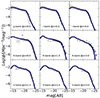 |
Fig. 1. Calibration set used for the CR-IGIMF run. The gray points represent the galaxy luminosity functions in different wavebands and at different redshifts, including the SDSS g, r, and i band, K, and V band (the same compilation of observational estimates used in F17 and F18a; see these papers for detailed references). In all panels, the blue line refers to the reference model predictions. |
Parameter calibration chart.
As discussed in the previous paragraph, the assumption of a variable IMF requires an additional layer in the analysis because it introduces a mismatch between the intrinsic stellar mass M⋆ predicted by the model and the observational datasets, which are usually derived assuming a universal IMF. Therefore, in order to provide a quantitative comparison between the predictions of our model and existing observational estimates, we defined an “apparent” stellar mass ( ), using the same approach as in F17 and F18a, which we summarize in the following. Since our synthetic photometry is derived self-consistently from SSP models that considered the correct IMF of each star formation event, we can use this information to robustly estimate the stellar mass an observer would derive using magnitudes in different bands and assuming an MW-like IMF. In particular, we employed a theoretically derived4 relation between the mass-to-light ratio in the i band and the g − i color,
 (11)
(11)
with υ = 0.9 and δ = 0.7 (Zibetti, priv. comm., based on an analysis similar to Zibetti et al. 2009). An additional factor ϵ = 0.13 was introduced in F17 to account for spatial resolution effects (see F17a for a complete discussion of the origin and a justification of this shift).
4. Results
We first considered model predictions against a set of observational results that were previously tested in F17 and F18a in order to check the consistency of the new IMF variability scheme with our previous findings (Sects. 4.1 and 4.2). We then explored additional spectroscopic constraints to validate our proposed variability scenario (Sects. 4.3 and 4.4).
4.1. Stellar mass assembly
The resulting GSMFs at different redshifts computed using the intrinsic M⋆ and the apparent  are shown in Fig. 2. As shown and discussed in F17, the photometrically derived GSMF in a variable IMF scenario exhibits systematic deviations from the intrinsic GSMF, in particular, at low redshift (z < 1), where the growth of massive structures is apparently slowed down considering
  . At higher redshift, the main differences between the intrinsic GSMF and the GSMF defined using
  are found around the knee and at the low-mass end.
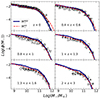 |
Fig. 2. Galaxy stellar mass function evolution as derived from different stellar mass estimates. The solid blue lines correspond to the estimate using the intrinsic stellar masses from the GAEA run. The dashed red lines show the predicted evolution using |

Intrinsic and apparent stellar masses for individual systems can be compared to assess the relevance of deviations from the MW-like IMF. In order to reproduce the same diagnostic as in observational samples, we considered bulge-dominated model galaxies, that is, a bulge-to-total stellar mass ratio (B/T) higher than 0.7. We tried to mimic the dynamical analysis of Cappellari et al. (2012) by considering the ratio of the true stellar mass-to-light ratio in the i band (M⋆/Li) and the apparent ratio (Eq. (11)) as a function of the proper M⋆/Li (right panel of Fig. 3). We also considered the M⋆/ ratio as a function of M⋆ (left panel of Fig. 3), which should correspond to Fig. 4 in Conroy et al. (2013). The predictions for the CR-IGIMF run (solid blue lines) agree qualitatively with observational results, showing an increase in the so-called α-excess with stellar mass and mass-to-light ratios. For reference, we also considered the predictions of the same quantities from our standard run (HDLF16; dashed black lines) adopting a universal MW-like IMF, which predicts flatter relations. These results confirm the conclusions of our previous work. As in F17, the positive α-excess at M⋆ > 1010 M⊙ (M⋆/Li > 0) is driven by variations in the IMF high-mass end (which is shallower than the Salpeter IMF in high-SFR events connected with the formation of massive ETGs). In particular, we do not interpret the α-excess in massive ETGs as a result of a typical IMF that is bottom-heavier than the MW-like, but instead as due to the mismatch between proper and synthetic mass-to-light ratios. Nonetheless, it is worth noting that the assumption that the low-mass end can vary as well (as in our CR-IGIMF scenario) does not increase the maximum predicted values for the α-excess (and/or the normalization of the relation). We discuss this point in detail in Sect. 4.3. The main difference with the standard IGIMF case is found at the low end of the mass-to-light ratio in the right panel. In the IGIMF scenario, the constancy of the low-mass end results in a flattening of the α-excess (see, i.e., Fig. 8 in F17), while the CR-IGIMF realization predicts an (almost) constant slope of the relation extending to negative α-excess values.
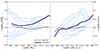 |
Fig. 3. α-excess as a function of stellar mass (left panel) and stellar mass-to-light ratio (right panel). In each panel, the solid blue and dashed black lines correspond to the predictions of the CR-IGIMF and the universal MW-like IMF runs, respectively; light blue contours mark galaxy number density levels (normalized to the maximum density) corresponding to 1%, 5%, 10%, and 25% in the CR-IGIMF run. |
4.2. Metallicities
We then considered the predicted evolution of the mass-metallicity relations (MZRs; both for for the gaseous component and the stellar component; see the left and right panels in Fig. 4, respectively). We compared the predictions from the CR-IGIMF run (solid blue line; the shaded area represents the 15−85th percentiles of the distributions) with the collection of observational estimates used in Fontanot et al. (2021, see that paper for a complete reference list). We also included predictions from our standard HDLF16 run (dashed black line). As discussed in Fontanot et al. (2021), we assumed a 0.1 dex shift downward of gas metallicities in order to obtain the correct normalization with respect to z ∼ 0 data and to better highlight the fact that our standard model is able to reproduce the redshift evolution of the gas MZR. It is worth noting that this assumed shift is still within the uncertainty in the normalization of the MZR (see, e.g., Kewley & Ellison 2008).
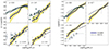 |
Fig. 4. Redshift evolution of the cold gas MZR (left panel – a downward 0.1 dex shift was applied to the predictions to match the overall normalization – see text for more details) and stellar MZR (right panel) relations. The lines and shaded areas refer to the CR-IGIMF and HDLF16 models as in Fig. 5. The data points correspond to the compilation used in Fontanot et al. (2021). |
The results shown in Fig. 4 clearly highlight that the CR-IGIMF run predicts an overall normalization of the MZR relations that agrees well with the observational estimates and with the universal IMF scenario. The main tensions are seen for gas metallicities of low-mass galaxies at z ∼ 0, and there is a clear overprediction of the stellar metallicities at z ∼ 3.5 (which is already present in the HDLF16 run). Nonetheless, the CR-IGIMF run systematically predicts steeper MZRs at z > 1 in the stellar and gaseous phases. The increase in metallicity is particularly relevant at M⋆ > 1010 M⊙, with model galaxies reaching (super-)solar metallicities even at considerable redshifts (z ∼ 2 − 3). These results for more massive galaxies differ from the observational estimates reported in Fig. 4. Nonetheless, some recent results suggest that at least a fraction of the most massive galaxies at z ∼ 3.4 already has supersolar metallicities (Saracco et al. 2020), which qualitatively agrees with the predictions of the CR-IGIMF scenario. Moreover, Saracco et al. (2023) recently reported no metallicity evolution for massive ETGs over the redshift range 0.0 < z < 1.4 (see also Vazdekis et al. 1997, and in particular, their Fig. 21).
We also verified that the CR-IGIMF run reproduced the [α/Fe]-stellar mass relation for ETGs reasonably well (which we selected in the model predictions by again applying the B/T > 0.7 criterion). In detail, we compared observational estimates for [α/Fe], calibrated using magnesium lines, against [O/Fe] theoretical predictions (since oxygen represents the most abundant α element). Figure 5 shows that the predictions for the CR-IGIMF run (solid blue line) are perfectly in line with our previous findings, showing that the IGIMF scenario naturally predicts an increase in [α/Fe] with stellar mass, at variance with the model assuming a universal MW-like IMF. In F17 (see their Fig. 7), we showed that the positive slope is a combination of (a) the increase in the α-enhancement for massive galaxies that is due to the shallower high-mass end slope (with respect to α2) associated with the high-SF events characterizing their early evolution, and (b) the predominance of IMFs that are bottom-heavier that the MW-like IMF in low-mass galaxies (leading to a decrease in the [α/Fe]).
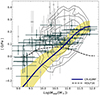 |
Fig. 5. [O/Fe] ratios in GAEA realization. The blue lines refer to the predictions of the CR-IGIMF, and the shaded area corresponds to the 15−85th percentiles. As reference, the dashed black lines show predictions from the HDLF16 model. Only model ETGs (i.e., B/T > 0.7) were considered. The observational constraints are taken from Thomas et al. (2010, contours), Arrigoni et al. (2010, dark gray circles), Spolaor et al. (2010, light gray squares). |
In this case, as for the α-excess, there is no relevant change in the results obtained within the CR-IGIMF framework with respect to the standard IGIMF scenario. We thus confirm all our previous conclusions about the impact of a variable IMF on the assembly of galaxy stellar masses and metallicities: Our interpretation still holds in the CR-IGIMF scenario. In the following, we consider additional spectroscopic constraints.
4.3. Dwarf-to-giant ratio
In order to determine whether the CR-IGIMF run can reproduce the observational finding of a bottom-heavy IMF in more massive galaxies at z ∼ 0, we computed for each model galaxy the IMF at z ∼ 0 and the corresponding dwarf-to-giant ratio, fdg. The fdg is defined as the ratio of the mass of stars below 0.6 M⊙ to that of stars below 1.0 M⊙ in the IMF. The reason for this normalization is that stars more massive than ∼1 M⊙ are already dead for old populations, and do not contribute to the integrated galaxy light (Martín-Navarro et al. 2019). The fdg was found to increase with galaxy velocity dispersion, reflecting the variation in the IMF slope La Barbera et al. (2013).
Figure 6 plots the relation between fdg and velocity dispersion, σ, for model galaxies in the CR-IGIMF run. As in Fig. 3 of F18b, σ was estimated using the relation between the velocity dispersion and stellar mass from Zahid et al. (2016). The green stars in the figure show the median in bins of σ. We note that in the CR-IGIMF framework, the MW-like IMF (i.e., UCR/UMW = 1 and SFR ∼ 1 M⊙ yr−1) has fdg = 0.718, slightly above the value for a Kroupa IMF (fdg = 0.713; see the figure). We find that fdg tends to increase (by 0.01 − 0.02) with σ, approaching the value for an MW IMF at σ ∼ 80 km s−1. The trend is consistent, although shallower, than that of F18b. Moreover, it is slightly clearer for in situ stars5, where fdg reaches a value as low as ∼0.72 at σ ∼ 80 km s−1 (in contrast to fdg ∼ 0.73, when all stars are considered). We stress that at variance with the preliminary analysis presented in F18b, we here analyzed a fully calibrated, self-consistent CR-IGIMF GAEA realization.
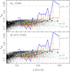 |
Fig. 6. Ratio of dwarf-to-giant stars in the IMF, fdg, plotted against the velocity dispersion of model galaxies, σ, for the CR-IGIMF run (black dots). The top and bottom panels are obtained by considering all stars in the model and those formed in situ, respectively. The green stars show the binned median trends, and the blue line corresponds to the IMF–σ relation from La Barbera et al. (2013). The orange circles with error bars show the latter relation corrected to an aperture of 1 Re, and the red line corresponds to an infinite aperture (see text). The expected fdg values for a Kroupa and Salpeter IMF are marked by dashed horizontal lines, and the dotted line marks the fdg for an MW-like IMF in the model. |
In order to compare the predicted fdg–σ trend with observations, we considered the relation obtained by La Barbera et al. (2013, see their Sect. 7) for the central regions of ETGs as observed by the SDSS (blue curve in Fig. 6). This evolves from a Kroupa-like distribution at σ ≲ 170 km s−1 to an fdg consistent or even steeper than that corresponding to a Salpeter IMF (fdg ∼ 0.84) at σ ∼ 300 km s−1. In order to perform a fair comparison with GAEA, we considered that the model predicts global quantities for each galaxy, while observations refer to the SDSS aperture. To perform an aperture correction, we assumed an IMF-radial profile as in La Barbera et al. (2017), where the IMF slope is bottom-heavy in the center and decreases to a Kroupa-like distribution at about the effective radius (Re). This trend is also consistent with the IMF radial profiles derived by van Dokkum et al. (2017). The IMF profile was normalized in each σ bin to match the IMF slope within the SDSS fiber aperture, and it was then used to recompute the IMF slope within a given aperture and the corresponding fdg value. The orange points and red lines in Fig. 6 show the fdg–σ relations corrected to 1 Re and an infinite aperture6, respectively. As expected, the relation flattens at a larger aperture. For an infinite aperture, the range of predicted values for fdg (green stars) is similar to the observed range. However, the model trend is still shallower than the observed trend. At high sigma (σ ∼ 300 km s−1), the model tends to underpredict fdg, while at 100 < σ < 220 km s−1, most model galaxies have fdg above the observed values. Therefore, our CR-IGIMF implementation appears to be unable to quantitatively reproduce the IMF–σ relation observed at z ∼ 0.
4.4. IMF-sensitive indices at z ∼ 0
In order to further compare predictions of the CR-IGIMF run with observations, we computed synthetic spectra and spectral indices for GAEA model galaxies. First, using the spectral synthesis code of Vazdekis et al. (2012), we computed a large library of SSP models with varying age, metallicity, and IMF. We only generated models in the optical spectral range, relying on the MILES stellar library (3540 < λ < 7410 Å; Sánchez-Blázquez et al. 2006) at a spectral resolution of 2.5 Å (FWHM; Falcón-Barroso et al. 2011). We note that the spectra used a different spectrophotometric synthesis code with respect to the code we used to calibrate the model (i.e., the updated version of BC03; see above). Nonetheless, since we used broadband photometry for the calibration, we do not expect significant differences between the two codes that might affect our conclusions. Generating synthetic spectra with the Vazdekis code allowed us to perform a more consistent comparison to results obtained from observed spectra using the same code (see, e.g., La Barbera et al. 2013). On the other hand, using BC03 for calibration, we can have a direct comparison with our previous results (F17 and F18a). We constructed SSPs based on Teramo isochrones, with ages in the range from 0.03 to 14 Gyr, and metallicities from [M/H] = −2.27 to +0.26 (see Vazdekis et al. 2015 for details). For each age and metallicity, SSPs were computed with the 42 different IMFs defined in Table 1, corresponding to seven (six) values of log(SFR) (UCR/UMW). For each model galaxy, we stored its full star formation history, consisting of the list of mass elements that form in all galaxy progenitors at different time steps of the simulation. In order to disentangle the effect of a variable IMF from that of the SFH in GAEA, we fixed for simplicity the age and metallicity of all elements to their mass-weighted values over the galaxy SFH. This should also allow us to perform a fairer comparison to observations, where the IMF is typically inferred by assuming a single SSP. For each element, we computed by linear interpolation the corresponding synthetic spectrum, given its age, metallicity, and IMF. The spectrum of each element was normalized to its stellar mass, and all elements were summed to produce the final synthetic spectrum of the galaxy.
Figure 7 (top panel) plots as an example the spectra of a high- (M⋆ = 11.3) and low- (M⋆ = 9) mass galaxy in the CR-IGIMF run, the former with an fdg of ∼0.75 (i.e., heavier than MW), and the latter with an MW-like IMF (fdg ∼ 0.71). The bottom panel of the figure shows the ratio of the two spectra to those obtained by assuming an MW IMF. For the low-mass galaxy, the ratio is close to one, as expected, while for the high-mass system, we see features typical of a more bottom-heavy IMF (see La Barbera et al. 2013), such as stronger NaD (λ ∼ 5900 Å) and TiO2SDSS (λ ∼ 6200 Å) absorptions and weaker CaH+K lines (λ ∼ 3900 Å). However, the effect is small, and the variations are below ∼1% for most of the spectrum. This is consistent with what was found in F18b based on a preliminary implementation of the CR-IGIMF framework.
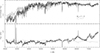 |
Fig. 7. Examples of synthetic MILES spectra (top panel) for two model galaxies in the CR-IGIMF run of GAEA. The black and gray curves correspond to a high- (M⋆ ∼ 11.3) and low-mass (M⋆ ∼ 9) galaxy, respectively. The bottom panel shows the ratio of each spectrum to that obtained for an MW IMF. Both spectra are at the nominal resolution of MILES (∼2.5 Å FWHM). |
In order to study the absorption features in more detail, we computed spectral indices from the synthetic spectra of all model galaxies. We focused on two prominent IMF-sensitive features in the optical spectral range, that is, TiO2SDSS and NaD, whose definitions, that is, central passband and pseudocontinua, were taken from La Barbera et al. (2013) and Trager et al. (1998), respectively. Figure 8 plots the difference of TiO2SDSS (top; δ(TiO2SDSS)) and NaD (bottom; δ(NaD)) with respect to the case of an MW IMF as a function of the galaxy velocity dispersion. Following the original definition of the Lick indices, NaD was computed in units of Å, while TiO2SDSS is given in magnitudes. The green stars represent median-binned trends for model galaxies, while red lines show the observed trends for the SDSS stacked spectra of La Barbera et al. (2013). The observed values of δ(TiO2SDSS) and δ(NaD) correspond to the case of an infinite aperture (see Fig. 6) and were obtained as follows. For a given stacked spectrum, we computed the TiO2SDSS and NaD indices for an SSP model with the age, metallicity, and IMF slope measured for the given spectrum (see La Barbera et al. 2013 for details). The IMF slope was corrected to an infinite aperture (see Sect. 4.3), while for the age and metallicity, we considered the values measured within the SDSS fiber aperture. Then we computed the difference of these line strengths with respect to the case where the IMF was set to an MW-like distribution, while age and metallicity were not varied. These differences give the red curves in Fig. 8. In the model, both NaD and TiO2SDSS tend to increase with σ, as expected from the behavior of fdg. However, the predicted variation is too small compared to the observations. For instance, at the highest σ (∼300 km s−1), the observed δ(NaD) is ∼0.12 Å, while for the model galaxies, it is only ∼0.02 Å on average. In order to understand this discrepancy, we recall that the strength of IMF-sensitive features in the optical is mostly driven by fdg, but to second order, it is also affected by the detailed shape of the IMF. For instance, using different IMF parameterizations (unimodal and low-mass tapered IMFs), LB13 showed that optical indices imply a similar trend of fdg with galaxy velocity dispersion, with small differences at fixed sigma between different parametrizations (see Fig. 19 of LB13). We found that the difference between the observed trends in Fig. 8 (red curves) and the model predictions (green stars) is twofold. At σ ∼ 300 km s−1, the average fdg of the CR-IGIMF run is ∼0.745, that is, lower than the observed value of ∼0.76 (for the case of an infinite aperture; see Fig. 6). However, assuming fdg = 0.745 and the same IMF parameterizations7 as in La Barbera et al. (2013), and following the same procedure adopted to derive the red curve in Fig. 8, we would infer a value of δ(NaD) ∼ 0.06 Å, which is lower than the estimate obtained from SDSS spectra, but still significantly higher than the value of ∼0.02 Å in the model (green stars in the figure). Therefore, we conclude that the discrepancy seen in Fig. 8 is due to the fact that the fdg–σ relation is too shallow in the models compared to the data and that the IMF shape in the CR-IGIMF framework is not able to produce a significant variation of the spectral features, as found in the data. We point out that the CR-IGIMF framework does not assume any direct scaling of the IMF with σ (or galaxy mass). As already discussed in F18b, the dependence on σ results from the competing effect of the increase in the SFR with galaxy mass (which leads to a higher fdg at fixed UCR; see, e.g., lines 4 to 7 or lines 11 to 14 in Table 1) and the UCR increase with galaxy mass (which favors lower fdg values; compare, e.g., lines 12, 19, and 26 in Table 1). The fact that the trends of δ(TiO2SDSS) and δ(NaD) with σ in Fig. 8 are too weak compared to the data implies that some further ingredient is still missing in the current implementation of the varying IMF framework. One possible solution would require an explicit scaling with σ, for instance, assuming a variation of the low-mass end of the IMF as a function of some physical parameter, such as metallicity (e.g., Jeřábková et al. 2018; Yan et al. 2024) and/or surface density (see Tanvir & Krumholz 2024), consistent with observational results (e.g., Martín-Navarro et al. 2015; La Barbera et al. 2019). Since more massive galaxies are also more metal rich and denser than their low-mass counterparts, we expect that this would produce a stronger increase in δ(TiO2SDSS) and δ(NaD) with σ by construction, as well as a stronger trend of fdg with galaxy mass. Nonetheless, an implementation like this is beyond the scope of the present work. We defer a more thorough investigation of the effect of these additional dependences to future work.
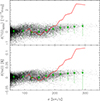 |
Fig. 8. Difference of the spectral indices between the case of variable and an MW-IMF for the model galaxies in the CR-IGIMF run (black dots). The top and bottom panel show the TiO2SDSS and NaD indices, respectively. The green stars show the binned trend, with error bars marking the 5th and 95th percentiles of the distribution in each bin. The red curves correspond to the observed trends from La Barbera et al. (2013), corrected to an infinite aperture (see text for more details). |
5. Conclusions
We have presented predictions for an updated version of the state-of-the-art semi-analytic model GAEA that implements our recently proposed variable IMF framework (CR-IGIMF). The CR-IGIMF scenario combines the integrated galaxy-wide IMF approach (see, e.g., Kroupa et al. 2013) with the results of high-resolution numerical simulations of star formation in giant molecular clouds (Papadopoulos et al. 2011). The main improvement with respect to the standard IGIMF approach lies in the fact that we allowed individual MCs to be characterized by different IMFs under the assumption that their characteristic Jeans mass depends on the cosmic-ray background in which they are embedded. As a result of our calculations, we showed in Fontanot et al. (2018b) that this approach is able to predict CR-IGIMF shapes that deviate from a universal MW-like IMF at the high- and low-mass ends at the same time. We deem this property very promising to explain several observational findings of a non-universal IMF in a self-consistent way, which are usually difficult to reconcile under a single top-heavy or a bottom-heavy IMF scenario. The coupling of the CR-IGIMF with GAEA allowed us to exploit the features of our galaxy formation model (and in particular, its improved modeling of chemical enrichment; De Lucia et al. 2014) to consider a variety of predictions for the physical, dynamical, chemical, and photometric properties of the model galaxies. For the purposes of this study, we also coupled GAEA with the spectral synthesis code by Vazdekis et al. (2010) in order to derive synthetic spectral energy distributions that self-consistently accounted for IMF variation. This allowed a direct comparison of synthetic spectral features with the observed ones.
We summarize our main conclusions below.
-
The CR-IGIMF scenario confirms our previous findings (F17 and F18a): The expected variability at the IMF high-mass end allows us to match the so-called α-excess, that is, the reported excess, with respect to expectations based on a universal IMF of the stellar mass and mass-to-light ratio derived from dynamical and spectroscopic studies. Moreover, our models are also able to correctly reproduce both the trend of increasing [α/Fe] with stellar mass and stellar mass-metallicity relations in the local Universe at the same time, which represents a long-standing problem for theoretical models (see, e.g., De Lucia et al. 2017).
-
At z ≳ 1, both the predicted stellar and cold-gas MZR are steeper than observational estimates. In particular, our model predicts substantial metallicities at the high-mass end (i.e., M⋆ > 1010 M⊙) already at intermediate redshift, in tension with the observed relations. Nonetheless, these predictions may explain recent findings of the supersolar metallicities for a sample of massive ETGs at z ≲ 3 (Saracco et al. 2023; D’Ago et al. 2023; Bevacqua et al. 2023).
-
The properties of synthetic spectral energy distributions for model ETG galaxies agree qualitatively with the results derived from observed spectra. In particular, our synthetic spectra show a similar increasing trend of the dwarf-to-giant ratio (fdg, i.e., the mass fraction in the IMF of stars with masses below 0.6 M⊙) as a function of galaxy velocity dispersion. Moreover, IMF-sensitive synthetic spectral features such as TiO2SDSS and NaD also show a slightly increasing trend with velocity dispersion. However, all these trends, despite showing the correct dependence on the velocity dispersion, are considerably weaker than observed, possibly demanding further developments of the CR-IGIMF framework.
Overall, our CR-IGIMF GAEA realization is able to reproduce at the same time a variety of observational findings based on dynamics, photometric and spectroscopic studies suggesting a time variability in the IMF of ETGs galaxies. This represents a fundamental step forward in our understanding of the overall impact of a variable IMF on galaxy properties and in constraining variability scenarios. The main problem of our current model lies in the fact that it is not able to reproduce the correct strength in the evolution of spectral features such as TiO2SDSS and NaD with velocity dispersion, although the predicted relations trend in the correct direction. It is important to stress that this is not a limitation of the IGIMF framework (and its extension, e.g., the CR-IGIMF), but is more tightly connected with the underlying assumptions. For example, our CR-IGIMF library is limited to low-mass end slopes that range between a Kroupa and a Salpeter IMF by construction, that is, we assumed that the IMFs associated with individual clouds cannot be steeper than a Salpeter IMF or shallower than a Kroupa IMF below 1 M⊙. Our results show that this might not be sufficient to reproduce the observed fdg trends as a function of velocity dispersion, although they typically range between these two extremes (see, e.g., Fig. 6). In order to obtain steeper slopes both for fdg and the spectral indices, we likely have to act at the level of IMF slopes in individual clouds. For example, more extreme IMF, super-Salpeter α1 ∼ −3 slopes have been suggested in La Barbera et al. (2016) to explain radial IMF trends in the innermost regions of local ETGs. The origin of these extreme IMF slopes depends on the physical conditions of star-forming regions (see, e.g., Chabrier et al. 2014), which may deviate largely from local counterparts in the MW environment, in particular, for molecular gas density and metallicity. We will explore the impact of a wider range of low-mass end slopes in future work.
Galaxy And Mass Assembly.
In Fontanot et al. (2018a) we assumed that the SFR surface density is a good tracer of the CR energy density.
The stellar feedback scheme assumes that gas reheating (and energy injection) follows the fitting formulae proposed by Muratov et al. (2015) and based on high-resolution hydro-simulations. The gas can be ejected from the halo following the same approach as in Guo et al. (2011). Finally, the gas can be reincorporated on a timescale that depends on halo mass, as in Henriques et al. (2013).
The relation was derived using a Monte Carlo library of 500 000 synthetic spectra based on the Bruzual & Charlot (2003) spectro-photometric code, assuming a Chabrier IMF and age-dependent dust attenuation (Zibetti et al. 2017).
We considered as stars formed in situ those that were formed in the main progenitor of the z ∼ 0 model galaxies, that is, that were not accreted from satellites in mergers.
In this case, we computed the luminosity-weighted value of the IMF slope within an infinite radius, assuming a Kroupa-like distribution outside one effective radius.
In particular, we adopted a low-mass tapered bimodal distribution, consisting of a single power law that was tapered at low mass through a spline, with the slope of the upper segment as the only free parameter.
Acknowledgments
We thank the anonymous referee for comments that helped us improve the quality of the presentation of our results. F.F. and F.L.B. acknowledge financial support from the INAF PRIN “ETGs12” (1.05.01.85.11). F.L.B. acknowledges support from the Institute for Fundamental Physics of the Universe (IFPU) for organizing a “Focus Week” where some of the work for this paper has been finalized. A.V. acknowledges support from grant PID2021-123313NA-I00 and PID2022-140869NB-I00 from the Spanish Ministry of Science, Innovation and Universities MCIU. We also acknowledge the computing centre of INAF-OATs, under the coordination of the CHIPP project (Taffoni et al. 2020), for the availability of computing resources and support. An introduction to GAEA, a list of our recent work, as well as datafile containing published model predictions, can be found at https://sites.google.com/inaf.it/gaea/home
References
- Arrigoni, M., Trager, S. C., Somerville, R. S., & Gibson, B. K. 2010, MNRAS, 402, 173 [NASA ADS] [CrossRef] [Google Scholar]
- Bevacqua, D., Saracco, P., La Barbera, F., et al. 2023, MNRAS, 525, 4219 [NASA ADS] [CrossRef] [Google Scholar]
- Bruzual, G., & Charlot, S. 2003, MNRAS, 344, 1000 [NASA ADS] [CrossRef] [Google Scholar]
- Cappellari, M., McDermid, R. M., Alatalo, K., et al. 2012, Nature, 484, 485 [Google Scholar]
- Chabrier, G. 2003, ApJ, 586, L133 [NASA ADS] [CrossRef] [Google Scholar]
- Chabrier, G., Hennebelle, P., & Charlot, S. 2014, ApJ, 796, 75 [Google Scholar]
- Conroy, C., & van Dokkum, P. G. 2012, ApJ, 760, 71 [Google Scholar]
- Conroy, C., Dutton, A. A., Graves, G. J., Mendel, J. T., & van Dokkum, P. G. 2013, ApJ, 776, L26 [NASA ADS] [CrossRef] [Google Scholar]
- D’Ago, G., Spiniello, C., Coccato, L., et al. 2023, A&A, 672, A17 [NASA ADS] [CrossRef] [EDP Sciences] [Google Scholar]
- De Lucia, G., & Blaizot, J. 2007, MNRAS, 375, 2 [Google Scholar]
- De Lucia, G., Tornatore, L., Frenk, C. S., et al. 2014, MNRAS, 445, 970 [Google Scholar]
- De Lucia, G., Fontanot, F., & Hirschmann, M. 2017, MNRAS, 466, L88 [NASA ADS] [CrossRef] [Google Scholar]
- De Lucia, G., Xie, L., Fontanot, F., & Hirschmann, M. 2020, MNRAS, 498, 3215 [NASA ADS] [CrossRef] [Google Scholar]
- Dib, S. 2023, ApJ, 959, 88 [NASA ADS] [CrossRef] [Google Scholar]
- Falcón-Barroso, J., Sánchez-Blázquez, P., Vazdekis, A., et al. 2011, A&A, 532, A95 [Google Scholar]
- Ferreras, I., La Barbera, F., de la Rosa, I. G., et al. 2013, MNRAS, 429, L15 [NASA ADS] [CrossRef] [Google Scholar]
- Ferreras, I., Weidner, C., Vazdekis, A., & La Barbera, F. 2015, MNRAS, 448, L82 [NASA ADS] [CrossRef] [Google Scholar]
- Fontanot, F., De Lucia, G., Monaco, P., Somerville, R. S., & Santini, P. 2009, MNRAS, 397, 1776 [NASA ADS] [CrossRef] [Google Scholar]
- Fontanot, F., De Lucia, G., Hirschmann, M., et al. 2017a, MNRAS, 464, 3812 [NASA ADS] [CrossRef] [Google Scholar]
- Fontanot, F., Hirschmann, M., & De Lucia, G. 2017b, ApJ, 842, L14 [Google Scholar]
- Fontanot, F., De Lucia, G., Xie, L., et al. 2018a, MNRAS, 475, 2467 [NASA ADS] [Google Scholar]
- Fontanot, F., La Barbera, F., De Lucia, G., Pasquali, A., & Vazdekis, A. 2018b, MNRAS, 479, 5678 [NASA ADS] [CrossRef] [Google Scholar]
- Fontanot, F., De Lucia, G., Hirschmann, M., et al. 2020, MNRAS, 496, 3943 [CrossRef] [Google Scholar]
- Fontanot, F., Calabrò, A., Talia, M., et al. 2021, MNRAS, 504, 4481 [CrossRef] [Google Scholar]
- Gunawardhana, M. L. P., Hopkins, A. M., Sharp, R. G., et al. 2011, MNRAS, 415, 1647 [NASA ADS] [CrossRef] [Google Scholar]
- Guo, Q., White, S., Boylan-Kolchin, M., et al. 2011, MNRAS, 413, 101 [Google Scholar]
- Guo, Q., White, S., Angulo, R. E., et al. 2013, MNRAS, 428, 1351 [NASA ADS] [CrossRef] [Google Scholar]
- Hennebelle, P., & Chabrier, G. 2008, ApJ, 684, 395 [Google Scholar]
- Henriques, B. M. B., White, S. D. M., Thomas, P. A., et al. 2013, MNRAS, 431, 3373 [NASA ADS] [CrossRef] [Google Scholar]
- Hirschmann, M., De Lucia, G., & Fontanot, F. 2016, MNRAS, 461, 1760 [Google Scholar]
- Jeřábková, T., Hasani Zonoozi, A., Kroupa, P., et al. 2018, A&A, 620, A39 [Google Scholar]
- Kewley, L. J., & Ellison, S. L. 2008, ApJ, 681, 1183 [Google Scholar]
- Klessen, R. S., Ballesteros-Paredes, J., Vázquez-Semadeni, E., & Durán-Rojas, C. 2005, ApJ, 620, 786 [NASA ADS] [CrossRef] [Google Scholar]
- Klessen, R. S., Spaans, M., & Jappsen, A.-K. 2007, MNRAS, 374, L29 [NASA ADS] [CrossRef] [Google Scholar]
- Kroupa, P. 2001, MNRAS, 322, 231 [NASA ADS] [CrossRef] [Google Scholar]
- Kroupa, P., & Bouvier, J. 2003, MNRAS, 346, 369 [NASA ADS] [CrossRef] [Google Scholar]
- Kroupa, P., Weidner, C., Pflamm-Altenburg, J., et al. 2013, Planets, Stars and Stellar Systems (Dordrecht: Springer Science+Business Media), 5, 115 [NASA ADS] [CrossRef] [Google Scholar]
- Krumholz, M. R. 2014, Phys. Rep., 539, 49 [Google Scholar]
- La Barbera, F., Ferreras, I., Vazdekis, A., et al. 2013, MNRAS, 433, 3017 [Google Scholar]
- La Barbera, F., Vazdekis, A., Ferreras, I., et al. 2016, MNRAS, 457, 1468 [Google Scholar]
- La Barbera, F., Vazdekis, A., Ferreras, I., et al. 2017, MNRAS, 464, 3597 [Google Scholar]
- La Barbera, F., Vazdekis, A., Ferreras, I., et al. 2019, MNRAS, 489, 4090 [Google Scholar]
- La Barbera, F., Vazdekis, A., Ferreras, I., & Pasquali, A. 2021, MNRAS, 505, 415 [NASA ADS] [CrossRef] [Google Scholar]
- Lada, C. J., & Lada, E. A. 2003, ARA&A, 41, 57 [Google Scholar]
- Marigo, P., Girardi, L., Bressan, A., et al. 2008, A&A, 482, 883 [NASA ADS] [CrossRef] [EDP Sciences] [Google Scholar]
- Marks, M., & Kroupa, P. 2012, A&A, 543, A8 [NASA ADS] [CrossRef] [EDP Sciences] [Google Scholar]
- Marks, M., Kroupa, P., Dabringhausen, J., & Pawlowski, M. S. 2012, MNRAS, 422, 2246 [NASA ADS] [CrossRef] [Google Scholar]
- Martín-Navarro, I., La Barbera, F., Vazdekis, A., Falcón-Barroso, J., & Ferreras, I. 2015, MNRAS, 447, 1033 [Google Scholar]
- Martín-Navarro, I., Lyubenova, M., van de Ven, G., et al. 2019, A&A, 626, A124 [Google Scholar]
- Muratov, A. L., Kereš, D., Faucher-Giguère, C.-A., et al. 2015, MNRAS, 454, 2691 [NASA ADS] [CrossRef] [Google Scholar]
- Narayanan, D., & Davé, R. 2013, MNRAS, 436, 2892 [NASA ADS] [CrossRef] [Google Scholar]
- Papadopoulos, P. P., Thi, W.-F., Miniati, F., & Viti, S. 2011, MNRAS, 414, 1705 [NASA ADS] [CrossRef] [Google Scholar]
- Pflamm-Altenburg, J., Weidner, C., & Kroupa, P. 2007, ApJ, 671, 1550 [NASA ADS] [CrossRef] [Google Scholar]
- Planck Collaboration XVI. 2014, A&A, 571, A16 [NASA ADS] [CrossRef] [EDP Sciences] [Google Scholar]
- Plat, A., Charlot, S., Bruzual, G., et al. 2019, MNRAS, 490, 978 [Google Scholar]
- Salpeter, E. E. 1955, ApJ, 121, 161 [Google Scholar]
- Sánchez, S. F., Barrera-Ballesteros, J. K., Lacerda, E., et al. 2022, ApJS, 262, 36 [CrossRef] [Google Scholar]
- Sánchez-Blázquez, P., Peletier, R. F., Jiménez-Vicente, J., et al. 2006, MNRAS, 371, 703 [Google Scholar]
- Saracco, P., Marchesini, D., La Barbera, F., et al. 2020, ApJ, 905, 40 [NASA ADS] [CrossRef] [Google Scholar]
- Saracco, P., La Barbera, F., De Propris, R., et al. 2023, MNRAS, 520, 3027 [NASA ADS] [CrossRef] [Google Scholar]
- Sarzi, M., Spiniello, C., La Barbera, F., Krajnović, D., & van den Bosch, R. 2018, MNRAS, 478, 4084 [Google Scholar]
- Spiniello, C., Trager, S., Koopmans, L. V. E., & Conroy, C. 2014, MNRAS, 438, 1483 [Google Scholar]
- Spolaor, M., Kobayashi, C., Forbes, D. A., Couch, W. J., & Hau, G. K. T. 2010, MNRAS, 408, 272 [Google Scholar]
- Springel, V., White, S. D. M., Jenkins, A., et al. 2005, Nature, 435, 629 [Google Scholar]
- Taffoni, G., Becciani, U., Garilli, B., et al. 2020, Astronomical Data Analysis Software and Systems XXIX, ASP Conf. Ser., 527, eds. R. Pizzo, E. R. Deul, J. D. Mol, Jelle. de Plaa & H. Verkouter (San Francisco: Astronomical Society of the Pacific), 307 [Google Scholar]
- Tanvir, T. S., & Krumholz, M. R. 2024, MNRAS, 527, 7306 [Google Scholar]
- Thomas, D., Maraston, C., Schawinski, K., Sarzi, M., & Silk, J. 2010, MNRAS, 404, 1775 [NASA ADS] [Google Scholar]
- Tortora, C., Romanowsky, A. J., & Napolitano, N. R. 2013, ApJ, 765, 8 [NASA ADS] [CrossRef] [Google Scholar]
- Trager, S. C., Worthey, G., Faber, S. M., Burstein, D., & González, J. J. 1998, ApJS, 116, 1 [Google Scholar]
- van Dokkum, P., Conroy, C., Villaume, A., Brodie, J., & Romanowsky, A. J. 2017, ApJ, 841, 68 [Google Scholar]
- Vazdekis, A., Peletier, R. F., Beckman, J. E., & Casuso, E. 1997, ApJS, 111, 203 [CrossRef] [Google Scholar]
- Vazdekis, A., Sánchez-Blázquez, P., Falcón-Barroso, J., et al. 2010, MNRAS, 404, 1639 [NASA ADS] [Google Scholar]
- Vazdekis, A., Ricciardelli, E., Cenarro, A. J., et al. 2012, MNRAS, 424, 157 [Google Scholar]
- Vazdekis, A., Coelho, P., Cassisi, S., et al. 2015, MNRAS, 449, 1177 [Google Scholar]
- Wang, J., De Lucia, G., Kitzbichler, M. G., & White, S. D. M. 2008, MNRAS, 384, 1301 [CrossRef] [Google Scholar]
- Weidner, C., & Kroupa, P. 2005, ApJ, 625, 754 [NASA ADS] [CrossRef] [Google Scholar]
- Weidner, C., Kroupa, P., & Larsen, S. S. 2004, MNRAS, 350, 1503 [CrossRef] [Google Scholar]
- Weidner, C., Kroupa, P., Pflamm-Altenburg, J., & Vazdekis, A. 2013, MNRAS, 436, 3309 [NASA ADS] [CrossRef] [Google Scholar]
- Xie, L., De Lucia, G., Hirschmann, M., Fontanot, F., & Zoldan, A. 2017, MNRAS, 469, 968 [Google Scholar]
- Xie, L., De Lucia, G., Hirschmann, M., & Fontanot, F. 2020, MNRAS, 498, 4327 [NASA ADS] [CrossRef] [Google Scholar]
- Yan, Z., Jerabkova, T., & Kroupa, P. 2017, A&A, 607, A126 [NASA ADS] [CrossRef] [EDP Sciences] [Google Scholar]
- Yan, Z., Jeřábková, T., & Kroupa, P. 2021, A&A, 655, A19 [NASA ADS] [CrossRef] [EDP Sciences] [Google Scholar]
- Yan, Z., Li, J., Kroupa, P., et al. 2024, arXiv e-prints [arXiv:2405.05308] [Google Scholar]
- Zahid, H. J., Geller, M. J., Fabricant, D. G., & Hwang, H. S. 2016, ApJ, 832, 203 [NASA ADS] [CrossRef] [Google Scholar]
- Zhang, Z.-Y., Romano, D., Ivison, R. J., Papadopoulos, P. P., & Matteucci, F. 2018, Nature, 558, 260 [Google Scholar]
- Zibetti, S., Charlot, S., & Rix, H. 2009, MNRAS, 400, 1181 [NASA ADS] [CrossRef] [Google Scholar]
- Zibetti, S., Gallazzi, A. R., Ascasibar, Y., et al. 2017, MNRAS, 468, 1902 [NASA ADS] [Google Scholar]
All Tables
All Figures
|
Fig. 1. Calibration set used for the CR-IGIMF run. The gray points represent the galaxy luminosity functions in different wavebands and at different redshifts, including the SDSS g, r, and i band, K, and V band (the same compilation of observational estimates used in F17 and F18a; see these papers for detailed references). In all panels, the blue line refers to the reference model predictions. |
| In the text | |
|
Fig. 2. Galaxy stellar mass function evolution as derived from different stellar mass estimates. The solid blue lines correspond to the estimate using the intrinsic stellar masses from the GAEA run. The dashed red lines show the predicted evolution using |
| In the text | |
|
Fig. 3. α-excess as a function of stellar mass (left panel) and stellar mass-to-light ratio (right panel). In each panel, the solid blue and dashed black lines correspond to the predictions of the CR-IGIMF and the universal MW-like IMF runs, respectively; light blue contours mark galaxy number density levels (normalized to the maximum density) corresponding to 1%, 5%, 10%, and 25% in the CR-IGIMF run. |
| In the text | |
|
Fig. 4. Redshift evolution of the cold gas MZR (left panel – a downward 0.1 dex shift was applied to the predictions to match the overall normalization – see text for more details) and stellar MZR (right panel) relations. The lines and shaded areas refer to the CR-IGIMF and HDLF16 models as in Fig. 5. The data points correspond to the compilation used in Fontanot et al. (2021). |
| In the text | |
|
Fig. 5. [O/Fe] ratios in GAEA realization. The blue lines refer to the predictions of the CR-IGIMF, and the shaded area corresponds to the 15−85th percentiles. As reference, the dashed black lines show predictions from the HDLF16 model. Only model ETGs (i.e., B/T > 0.7) were considered. The observational constraints are taken from Thomas et al. (2010, contours), Arrigoni et al. (2010, dark gray circles), Spolaor et al. (2010, light gray squares). |
| In the text | |
|
Fig. 6. Ratio of dwarf-to-giant stars in the IMF, fdg, plotted against the velocity dispersion of model galaxies, σ, for the CR-IGIMF run (black dots). The top and bottom panels are obtained by considering all stars in the model and those formed in situ, respectively. The green stars show the binned median trends, and the blue line corresponds to the IMF–σ relation from La Barbera et al. (2013). The orange circles with error bars show the latter relation corrected to an aperture of 1 Re, and the red line corresponds to an infinite aperture (see text). The expected fdg values for a Kroupa and Salpeter IMF are marked by dashed horizontal lines, and the dotted line marks the fdg for an MW-like IMF in the model. |
| In the text | |
|
Fig. 7. Examples of synthetic MILES spectra (top panel) for two model galaxies in the CR-IGIMF run of GAEA. The black and gray curves correspond to a high- (M⋆ ∼ 11.3) and low-mass (M⋆ ∼ 9) galaxy, respectively. The bottom panel shows the ratio of each spectrum to that obtained for an MW IMF. Both spectra are at the nominal resolution of MILES (∼2.5 Å FWHM). |
| In the text | |
|
Fig. 8. Difference of the spectral indices between the case of variable and an MW-IMF for the model galaxies in the CR-IGIMF run (black dots). The top and bottom panel show the TiO2SDSS and NaD indices, respectively. The green stars show the binned trend, with error bars marking the 5th and 95th percentiles of the distribution in each bin. The red curves correspond to the observed trends from La Barbera et al. (2013), corrected to an infinite aperture (see text for more details). |
| In the text | |
Current usage metrics show cumulative count of Article Views (full-text article views including HTML views, PDF and ePub downloads, according to the available data) and Abstracts Views on Vision4Press platform.
Data correspond to usage on the plateform after 2015. The current usage metrics is available 48-96 hours after online publication and is updated daily on week days.
Initial download of the metrics may take a while.