| Issue |
A&A
Volume 577, May 2015
|
|
|---|---|---|
| Article Number | A22 | |
| Number of page(s) | 16 | |
| Section | Interstellar and circumstellar matter | |
| DOI | https://doi.org/10.1051/0004-6361/201424550 | |
| Published online | 24 April 2015 | |
Testing protostellar disk formation models with ALMA observations
1
Leiden Observatory, Leiden University,
Niels Bohrweg 2,
2300 RA
Leiden,
The Netherlands
e-mail:
harsono@strw.leidenuniv.nl
2
SRON Netherlands Institute for Space Research,
PO Box 800, 9700 AV
Groningen, The
Netherlands
3
Max-Planck-Institut für extraterretrische Physik,
Giessenbachstrasse 1,
85748
Garching,
Germany
4
Astronomy Department, University of Virginia,
Charlottesville, VA, USA
5
Niels Bohr Institute, University of Copenhagen,
Juliane Maries Vej 30,
2100
Copenhagen Ø,
Denmark
6
Centre for Star and Planet Formation, Natural History Museum of
Denmark, University of Copenhagen, Øster Voldgade 5-7, 1350
Copenhagen K,
Denmark
Received: 7 July 2014
Accepted: 6 January 2015
Context. Recent simulations have explored different ways to form accretion disks around low-mass stars. However, it has been difficult to differentiate between the proposed mechanisms because of a lack of observable predictions from these numerical studies.
Aims. We aim to present observables that can differentiate a rotationally supported disk from an infalling rotating envelope toward deeply embedded young stellar objects (Menv>Mdisk) and infer their masses and sizes.
Methods. Two 3D magnetohydrodynamics (MHD) formation simulations are studied with a rotationally supported disk (RSD) forming in one but not the other (where a pseudo-disk is formed instead), together with the 2D semi-analytical model. We determine the dust temperature structure through continuum radiative transfer RADMC3D modeling. A simple temperature-dependent CO abundance structure is adopted and synthetic spectrally resolved submm rotational molecular lines up to Ju = 10 are compared with existing data to provide predictions for future ALMA observations.
Results. The 3D MHD simulations and 2D semi-analytical model predict similar compact components in continuum if observed at the spatial resolutions of 0.5–1″ (70–140 AU) typical of the observations to date. A spatial resolution of ~14 AU and high dynamic range (>1000) are required in order to differentiate between RSD and pseudo-disk formation scenarios in the continuum. The first moment maps of the molecular lines show a blue- to red-shifted velocity gradient along the major axis of the flattened structure in the case of RSD formation, as expected, whereas it is along the minor axis in the case of a pseudo-disk. The peak position-velocity diagrams indicate that the pseudo-disk shows a flatter velocity profile with radius than does an RSD. On larger scales, the CO isotopolog line profiles within large (>9″) beams are similar and are narrower than the observed line widths of low-J (2–1 and 3–2) lines, indicating significant turbulence in the large-scale envelopes. However a forming RSD can provide the observed line widths of high-J (6–5, 9–8, and 10–9) lines. Thus, either RSDs are common or a higher level of turbulence (b ~ 0.8 km s-1) is required in the inner envelope compared with the outer part (0.4 km s-1).
Conclusions. Multiple spatially and spectrally resolved molecular line observations can differentiate between the pseudo-disk and the RSD much better than continuum data. The continuum data give a better estimate of disk masses, whereas the disk sizes can be estimated from the spatially resolved molecular lines observations. The general observable trends are similar between the 2D semi-analytical models and 3D MHD RSD simulations.
Key words: stars: formation / accretion, accretion disks / radiative transfer / line: profiles / magnetohydrodynamics (MHD) / methods: numerical
© ESO, 2015
1. Introduction
The formation of stars and their planetary systems is linked through the formation and evolution of accretion disks. In the standard star formation picture, the infalling material forms an accretion disk simply from angular momentum conservation (e.g., Lin & Pringle 1990; Bodenheimer 1995; Belloche 2013). However, magnetic field strengths observed toward molecular cores (see Crutcher 2012, for a recent review) are expected theoretically to be sufficient in affecting the formation and evolution of disks around low-mass stars (e.g., Galli et al. 2006; Joos et al. 2012; Krumholz et al. 2013; Li et al. 2013, 2014a). Recent advances in both observational and theoretical studies give an opportunity to test the star formation process at small scales (<1000 AU).
It has been known for a long time that the presence of magnetic fields can drastically change the flow dynamics around low-mass stars (e.g., Galli & Shu 1993) and potentially suppresses disk formation (e.g., Galli et al. 2006). The latter is due to catastrophic magnetic braking where essentially all of the angular momentum of the accreting material is removed by twisted field lines. Recently, Li et al. (2011) investigated the collapse and disk formation from a uniform cloud, while Joos et al. (2012) and Machida & Matsumoto (2011) performed simulations starting with a steep density profile and a Bonnor-Ebert sphere, respectively. They found that rotationally supported disks (RSDs) do not form out of uniform and non-uniform cores under strong magnetic fields unless the field is misaligned with respect to the rotation axis (Hennebelle & Ciardi 2009). Turbulence has also been shown to help with disk formation (Santos-Lima et al. 2012; Seifried et al. 2012; Myers et al. 2013; Joos et al. 2013; Li et al. 2014b).
In spite of a number of disk formation and evolution simulations, only a few observables have been presented so far. The expected observables in the continuum (spectral energy distribution or SED) from 1D and 2D disk formation models have been presented in Young & Evans (2005) and Dunham et al. (2010). Continuum observables out of 2D hydrodynamics simulations with a thin disk approximation have been shown by Dunham & Vorobyov (2012) and Vorobyov et al. (2013). However, only a handful of synthetic observables from 3D magnetohydrodynamics (MHD) simulations have been presented in the literature (e.g., Commerçon et al. 2012a,b).
Continuum observations probe the dust thermal emission and the dust structure around the protostar. However, high spatial and spectral resolution molecular line observations are needed to probe the kinematical structure as the disk forms. The aim of this paper is to present high-spatial (down to 0.1″ or 14 AU at a typical distance of 140 pc) synthetic observations of continuum and molecular lines from two of the 3D MHD collapse simulations presented in Li et al. (2013). The two simulations differ in the initial magnetic field direction with respect to the rotation axis: aligned and strongly misaligned where the magnetic field vector is perpendicular to the rotation axis. The two cases represent the two extremes of the field orientation. The synthetic observations will be compared with those from a 2D semi-analytical disk formation model presented in Visser et al. (2009) to investigate whether the predicted observables differ. The 2D models allow us to simplify the different input parameters of the MHD simulations into two parameters: sound speed (cs) and rotation rate. Rotational transitions of CO are simulated to trace the observable kinematical signatures.
Another motivation in simulating CO molecular lines is the availability of high-quality spectrally and spatially resolved observational data toward embedded young stellar objects (YSOs) on larger scales (>1000 AU). Spectrally resolved lines have been obtained for low-excitation transitions Ju ≤ 7 (Eu = 155 K) using ground-based facilities (e.g., Jørgensen et al. 2002; van Kempen et al. 2009a,b) and higher excited lines up to Ju = 16 (Eu = 660 K) using Herschel-HIFI (de Graauw et al. 2010) in beams of 9–20″ (Yıldız et al. 2010, 2013; Kristensen et al. 2013). Interestingly, San Jose-Garcia et al. (2013) find that the C18O 9–8 lines are broader than the 3–2 lines for low-mass YSOs. The observed line widths are greater than expected from the thermal broadening, which indicates a significant contribution of microscopic turbulence or some other forms of motion, such as rotation and infall. Through the characterization of spectrally resolved molecular lines on such physical scales, we aim to test the kinematics predicted in various star and disk formation models.
Another key test of star formation models is to compare the predicted mass evolution from the envelope to the star with observations (e.g., Jørgensen et al. 2009; Li et al. 2014a). Inferring these properties toward embedded YSOs is not straightforward owing to the confusion between disk and envelope. The mass evolution of the disk and envelope can be deduced from millimeter surveys that combine both aperture synthesis and single-dish observations (Keene & Masson 1990; Terebey et al. 1993; Looney et al. 2003; Jørgensen et al. 2009; Enoch et al. 2011). However, precise determination of stellar masses requires spatially and spectrally resolved molecular line observations of the velocity gradient in the inner regions of embedded YSOs (Sargent & Beckwith 1987; Ohashi et al. 1997; Brinch et al. 2007; Lommen et al. 2008; Jørgensen et al. 2009; Takakuwa et al. 2012; Yen et al. 2013). Here we apply a similar analysis to the synthetic continuum and molecular line data as performed on the observations to test the reliability of the inferred masses.
This paper is structured as follows. Section 2 describes the simulations and the radiative transfer method that are used. The synthetic continuum images are presented in Sect. 3. Section 4 presents the synthetic CO moment maps and line profiles for the different simulations. The results are then discussed in Sect. 5 and summarized in Sect. 6.
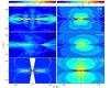 |
Fig. 1 Density and dust temperature structures in the inner 200 AU radius for all three simulations at t ~ 1.2 × 10⁵ years. Temperature contours at 25 K and 40 K are indicated in the right panels. Top: a vertical slice (R − z slice at φ = 0 where R denotes the cylindrical radial coordinate) of the 3D MHD simulation of RSD formation. Middle: a vertical slice of the 3D MHD simulation of a pseudo-disk (no RSD). Bottom: 2D semi-analytical disk formation model. The red lines highlight the region of the stable RSD. |
 |
Fig. 2 Velocity streamlines for the two MHD simulations in Li et al. (2013). The simulations are rendered with paraview (http://www.paraview.org). Left: 3D MHD simulation of a collapsing uniform sphere with the magnetic field vector perpendicular to the rotation axis. Right: The simulation with magnetic field vector aligned with the rotation axis. The color of the arrows indicate the azimuthal velocity vector, υφ, in km s-1. The solid black arrows indicate the general stream lines in the two simulations. The dark shaded colors indicate the density isocontours of nH2 = 107.5 cm-3 up to 1010.5 cm-3 (red). |
2. Numerical simulations and radiative transfer
2.1. Magnetohydrodynamical simulations
We utilize the 3D MHD simulations of the collapse of a 1 M⊙ uniform, spherical envelope as described in Li et al. (2013). The envelope initially has a density of ρ0 = 4.77 × 10⁻¹⁹ g cm-3, a solid-body rotation of Ω0 = 10-13 Hz, and a relatively weak, uniform magnetic field of B0 = 11 μG (λ = 10 where λ is the dimensionless mass-to-flux ratio). The details of the simulations can be found in Li et al. (2013).
A snapshot of two simulations at t = 3.9 × 10¹² s = 1.24 × 10⁵ years is used. This corresponds to near the end of the Stage 0 phase of star formation where almost one half of the initial core mass has collapsed onto the star (Robitaille et al. 2006; Dunham et al. 2014). The difference between the two simulations is the tilt angle between the rotation axis and the direction of initial magnetic field vector, θ0. One simulation starts with an initial tilt angle θ0 = 0° in which a pseudo-disk forms but not an RSD. The other simulation starts with an initial tilt angle of θ0 = 90° in which an RSD forms (see Fig. 1 and Fig. 1 in Li et al. 2013).
The RSD simulation (left) forms a flattened structure with number gas densities nH2> 106.5 cm-3 in the inner 300 AU radius. In the region r> 100 AU, the magnitude of the radial and azimuthal velocities are within a factor of 2 of each other. The radial velocities nearly vanish in the inner 70 AU radius (see Fig. 3). The streamlines in the RSD simulation show a coherent flattened rotating component (see Fig. 2). In the case of the pseudo-disk simulation, number densities of nH2> 106.5 cm-3 encompass r< 700 AU regions, which is a factor of 2 larger than the RSD simulation. An outflow cavity is present in this simulation with an expanding velocity field as shown in Fig. 1 (Left) of Li et al. (2013). The cavity is more evacuated compared with the one in the simulation simulation that forms a rotationally supported disk, although still not a canonical definition of a cavity. The magnitudes of the radial velocities are much greater than the azimuthal velocities in the inner r< 300 AU along most φ directions. In this simulation, the streamlines show infalling material straight from the large-scale envelope onto the forming star. Using these two simulations with very different outcomes, we can investigate the similarities and differences in both continuum and molecular line profiles for pseudo disk and RSD formation in 3D.
2.2. Semi-analytical model
For comparison, synthetic images from 2D semi-analytical axisymmetric models of collapsing rotating envelope and disk formation as described in Visser et al. (2009) with modifications introduced in Visser & Dullemond (2010) and Harsono et al. (2013) are also simulated. These models are based on the collapse and disk formation solutions of Terebey et al. (1984) and Cassen & Moosman (1981) including a prescription for an outflow cavity. The disk evolution follows the α-disk formalism as described in Shakura & Sunyaev (1973) and Lynden-Bell & Pringle (1974). The disk surface is defined by hydrostatic equilibrium as described in Visser & Dullemond (2010) and is assumed to be in Keplerian rotation. To compare with the MHD simulations, we consider the collapse of the 1 M⊙, cs = 0.26 km s-1, and Ω0 = 10-13 Hz core. The sound speed in this case is higher than the value used in Li et al. (2013), which affects the final disk properties at the end of the formation process. The synthetic observables are produced at t = 3.9 × 10¹² s. The bottom of Fig. 1 shows the physical structure of the 2D semi-analytical model at the time when a ~65 AU radius RSD is present.
A major difference between the 2D semi-analytical axisymmetric model and the 3D simulations is the outflow cavity. The photon propagation is still treated in 3D. Although outflowing gas is present in the pseudo-disk simulation (no RSD), the cavity remains filled with high number density (105 cm-3) gas, while lower density (102−3 cm-3) gas occupies the cavity in the 2D model. The outflowing gas generated from angular momentum conserving gas in the pseudo-disk model has relatively low velocities so that it does not clear out the cavity. As a result, the dust temperature along the cavity wall is higher in the 2D model owing to the direct illumination of the central star. This is readily seen in the 40 K contour in Fig. 1 where it is elongated in the z direction in the 2D case. However, we show in Sect. 4 that this difference does not affect the results of this paper.
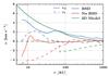 |
Fig. 3 Radial (solid) and azimuthal velocities (dashed) at the midplane (θ = π/ 2, φ = 0) for the three different models: 3D RSD MHD simulation (blue), 3D no RSD (red), and 2D model (green). |
Stellar (M⋆), envelope (Menv), and disk (Md) masses for the three simulations.
2.3. Rotationally supported disk sizes and masses
The extent of the RSD in the 2D semi-analytical model is defined by hydrostatic equilibrium. Using these properties, the RSD is defined by a region with densities >107.5 cm-3 and azimuthal velocities υφ> 1.2 km s-1. The disk evolution in 2D follows the alpha-disk formalism with α = 10-2, which in turns define the radial velocities as υr/υφ ~ α(H/R)2 ~ 10-3 where H is the disk’s scale height. Similar criteria are used to extract the extent of the RSD in the 3D simulation with the additional constraint of vφ>vr. We apply the criteria from the 2D model to define the RSD in the 3D simulation, thus it is is not necessarily in hydrostatic equilibrium. This can be clearly seen in Fig. 3 for the 3D simulation where υr/υθ does not satisfy the hydrostatic disk criterion along a few azimuthal angles. Using these criteria, an RSD up to 260 AU is found in the misaligned simulation. The extent of the 3D RSD is 300 AU if vφ> 1 km s-1 is used. With the former criterion, the disk masses contained within such a region are 0.06 M⊙ for the 3D RSD and 0.04 M⊙ for the 2D RSD surrounding 0.38 M⊙ and 0.35 M⊙ stars, respectively (see Table 1). As Fig. 3 shows, the radial velocity component of the pseudodisk is a significant fraction of the Keplerian velocity. Owing to such high radial velocities, the surface density of the pseudodisk remains low. However, the total mass of the high-density regions (nH2> 107.5 cm-3) is a factor of 2 higher than the RSD mass.
2.4. Observables and radiative transfer
The first step before producing observables is to calculate the dust temperature structure, which is critical for the molecular abundances since it controls the freeze-out from the gas onto the dust. The dust temperature is computed using the 3D continuum radiative transfer code RADMC3D1 with a central temperature of 5000 K, which is the typical central temperature in the 2D semi-analytical models near the end of Stage 0 phase. The central luminosity is fixed at 3.5 L⊙ for all models. The dust opacities used are those corresponding to a mix of silicates and graphite grains covered by ice mantles (Crapsi et al. 2008). The 3D MHD simulation from Li et al. (2013) has an inner radius of 1014 cm (6.7 AU), while the semi-analytical model has an inner radius of 0.1 AU. The simulated observables presented here are not sensitive to the physical and chemical structures in the inner 10 AU radius. Thus, these differences do not affect the conclusions of this paper. The same opacities and central temperature were adopted for all simulations in order to focus on the general features of the observables. The gas temperatures are assumed to be equal to the dust temperatures, which is valid for the optically thin lines simulated here that trace the bulk mass where Tgas ~ Tdust (Doty et al. 2002; Doty et al. 2004).
CO abundance.
In this paper, we concentrate on simulating CO molecular lines of J = 2–1, 3–2, 6–5, and 9–8. For simplicity, the 12CO abundance is set to a constant value of 10-4 with respect to H2 except in regions with Tdust< 25 K, where it is reduced by a factor of 20 to mimic freeze-out (Jørgensen et al. 2005; Yıldız et al. 2013). We adopt constant isotopic ratios of 12C/13C = 70, 16O/18O = 540, and 18O/17O = 3.6 (Wilson & Rood 1994) to compute the abundance structures of the isotopologs.
Synthetic images.
This paper presents synthetic continuum maps at 450, 850, 1100, and 1300 μm. The images are rendered using RADMC3D with an image size of 8000 AU on scales of 5 AU pixels. They are placed at a distance of 140 pc. Synthetic images at inclinations of 0° (face-on; down the z-axis), 45°, and 90° are produced. The last option is included because one of the claimed embedded disk sources is close to edge-on (i ~ 90°, L1527 in Tobin et al. 2012). For the synthetic molecular lines, the local thermal equilibrium (LTE) population levels are computed using the partition functions adopted from the HITRAN database (Rothman et al. 2009). LTE is a good assumption because the densities in the simulations are greater than the critical densities of the simulated transitions. Non-LTE effects may play a minor role for synthetic Ju ≥ 6 lines from the pseudo-disk simulation because of its lower densities relative to the other two simulations. The line optical depth (τL) is also not expected to play a role since the focus of this paper is on the minor isotopologs and on the kinematics dominated by the line wings where their line optical depths are lower than at the line center. The properties of the molecules (Eup and Aul) are taken from the LAMDA database (Schöier et al. 2005). Only thermal broadening is included in simulating the molecular lines without any additional microturbulence. The image cubes are rendered at a spectral resolution of 0.1 km s-1 covering velocities from −7.5 to 7.5 km s-1. To simulate observations, the synthetic images are then convolved with Gaussian beams between 0.1″ to 20″. The convolution is performed in the Fourier space with normalized Gaussian images.
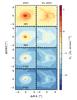 |
Fig. 4 Continuum intensity maps of 450, 850, 1100, and 1300 μm for the MHD disk formation simulation (left panels) and pseudo-disk (no RSD, right panels) at i = 45° at 5 AU pixels. Note the high dynamic range needed to see all of the structures. |
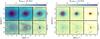 |
Fig. 5 Convolved continuum maps in the inner 5″ of 450 (left) and 1100 (right) μm at i = 45°. The images are convolved with 1″, 0.5″, and 0.1″ beams as indicated in each panel. For each panel, the top row shows synthetic image of RSD simulation and the pseudo-disk simulation is shown in the bottom row. The color scale presents the full range of the emission above 10-2 mJy/bm, not all of which may be detectable. Solid red contours are drawn from 3σ up to maximum at 6 logarithmic steps where 1σ is 0.01 × the maximum (dynamical range of 100) with a minimum at 0.5 mJy/bm for the 1″ and 0.5″ images. For the images convolved with a 0.1″ beam, the red contours are drawn with a minimum noise level of 0.5 mJy/bm for 450 μm and 0.05 mJy/bm at longer wavelengths with a dynamic range of 1000, as appropriate for the full ALMA. |
3. Continuum
3.1. Images and prospects for ALMA
Continuum images are rendered at four wavelengths and viewed at three different inclinations. Figure 4 presents the synthetic 450, 850, 1100, and 1300 μm continuum images at an inclination of 45° for the two 3D MHD simulations. The lefthand panels present the images from 3D RSD simulation, while the righthand ones show images from the pseudo-disk simulation (labeled as No RSD). The features produced during the collapse are clearly visible in the 450 μm map, with most of them two orders of magnitude fainter at 1300 μm. The spiral structure in the 450 μm image is due to magnetically channelled, supersonically collapsing material on its way to the RSD, rather than a feature of the RSD itself.
One of the aims of this paper is to investigate whether these features are observable with current observational limits and what is possible with future Atacama Large Millimeter/submillimeter Array (ALMA) data. With the full ALMA, a sensitivity of σ = 0.5 mJy bm-1 (bm = beam) at ~450 μm and 0.05 mJy bm-1 at 1100 μm can be achieved at spatial resolutions ≤0.1″ for 30 min of integration (1.8 GHz bandwidth). In addition, a high dynamic range of >1000 (σ = 0.001 × Speak) can also be achieved. Figure 5 presents the images convolved with a 0.1″ beam for the two 3D MHD simulations (rightmost panels). The color scale indicates the full range of emission, while the red solid lines show the region above 3σ where σ is either dynamically limited to 1000 or to the σ values listed above. This simply means that these lines indicate the detectable features. With a combination of high dynamic range and sensitivity, the features of the collapse are observable and distinguishable in both 450 μm and 1100 μm continuum maps. At a spatial resolution of 0.1″, most of the emission at 1100 μm is due to the rotationally supported disk with a small contribution from the surrounding envelope.
As Figs. 4 and 5 show, both the strength of the features and their extent change with wavelength, as indicated by the red line contours. With a resolution of 0.1″, the extent of the detectable emission decreases from 1.5″ at 450 μm to <1″ at 1100 μm for the RSD case. At long wavelengths, the dust emission is given by Iν ~ Tdustν2 × (1−e− τdust). Since the dust emission is optically thin at long wavelengths, the intensity is ∝Tdustν2τdust. The variables that depend on position are Tdust and τdust ∝ ρdustκν. The frequency dependence of the opacity is κν ∝ ν1.5 for the adopted opacity table. The extent of the detectable emission depends on these quantities. At one particular position, the ratio of the emission at the two wavelengths is simply I450 μm/I1100 μm ∝ ν3.5. Thus, the predicted difference in size at the two wavelengths is due to the frequency dependence of the emission.
For ALMA early science observations (cycles 0 and I), the capabilities provided a dynamic range only up to 100 at a spatial resolution of ~0.5″. Figure 5 presents synthetic 450 and 1100 μm images convolved with 1″ and 0.5″ beams, compared with the 0.1″ beam images. The color scale again indicates the full range of emission, while the red solid lines now show the region above 3σ where the noise level, σ, is dynamically limited to 100 with a minimum of 0.5 mJy/beam at both wavelengths. These lines again present the observable emission. The 450 μm images convolved with a 1″ beam show an elongated flattened structure for both RSD and pseudo-disk simulations and are therefore indistinguishable. Most of the emission at 1100 μm and longer wavelengths is not detectable at the assumed noise level of 0.5 mJy bm-1. A similar result is found after convolution with a 0.5″ beam. Although the synthetic observations from the pseudo-disk indicate a “cometary” structure, this may be affected by the presence of outflow cavity that is absent in the case of RSD. Thus, the full ALMA capabilities are needed to distinguish models based on continuum data alone.
3.2. Inclination effects
The images for a face-on system (i = 0°) are similar to those of the moderately inclined system (i = 45°) presented in Fig. 5. For low inclinations between 0 to 45°, the continuum images only change slightly in terms of absolute flux density and show a small elongation due to orientation.
In contrast, the two simulations rendered at edge-on (i ~ 90°) geometry exhibit similar compact components even at the highest angular resolution (Fig. 6). They both show an elongated flattened disk-like emission similar to the 2D semi-analytical model. This signature suggests an RSD, but it is due to the pseudo-disk produced in the 3D MHD simulation whose initial magnetic field vector is aligned with rotation axis. The peak continuum emission of the pseudo-disk is a factor of 10 lower than that of the other two models, while it is similar between the 3D RSD and the 2D semi-analytical models (difference of <10%). The main difference is the extent of the elongated emission where the 2D model predicts a very compact (~1″ radius) structure, and the pseudo-disk component shows an extended flattened structure (≤2″). This illustrates the difficulties in testing disk formation models for highly inclined systems based solely on continuum data.
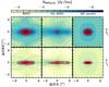 |
Fig. 6 Synthetic 850 μm continuum images convolved with 0.5″ (top) and 0.1″ (bottom) beams for the three simulations viewed at 90° (edge-on): RSD formation (left), pseudo-disk (center), and 2D semi-analytical model (right). The red solid lines are drawn at the same contours as in Fig. 5. |
4. Molecular lines
The continuum emission arises from thermal dust emission and does not contain kinematical information. As shown in the previous section, a compact flattened structure is expected in the continuum maps in the inner regions of all three models. Kinematical information as contained in spectrally resolved molecular lines is essential for distinguishing the models and deriving stellar masses. The rotational lines of CO isotopologs are used to investigate this.
The rotational lines of 13CO, C18O, and C17O were simulated. CO was chosen since its abundance is less affected by chemical evolution during disk formation. We did not investigate 12CO lines since they are dominated by the entrained outflow material and are optically thick. The isotopolog lines are more optically thin and are expected to probe the higher density region where the disk is forming. These predicted spatially resolved molecular line maps can be compared with ALMA data. Moreover, high-quality, spectrally resolved CO isotopolog lines probing the larger-scale envelope toward low-mass embedded YSOs have been obtained with single-dish telescopes (see Sect. 1). The characterization of these C18O and C17O line profiles test the kinematical and density structures of the collapsing protostellar envelope on larger scales (e.g., Hogerheijde et al. 1998; Jørgensen et al. 2002).
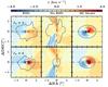 |
Fig. 7 First moment maps of C18O 2–1 (top) and 6–5 (bottom) for the three simulations viewed i = 45° convolved with a 0.1″ beam. The solid line shows the 20% intensity contour of the moment zero ( |

4.1. Moment maps: RSDs or not?
Observationally, the kinematical information of the infalling envelope and RSD is inferred through moment maps. Elongated zeroth moment (velocity integrated intensity) maps indicate the presence of a flattened structure that is associated with a disk. Meanwhile, coherent velocity gradients in the first moment (velocity weighted intensity) map may point to a rotating component. Analysis of synthetic moment maps of the simulations are presented and compared in this section. We focus on presenting the synthetic “interferometric” maps of optically thin C18O and C17O lines by convolving the image cubes with a 0.1″ Gaussian beam. The construction of moment maps only takes emission >1% of the peak emission into account. This translates into a noise level of 0.3% of the peak emission. Although ALMA can achieve a dynamic range of >500, it is more likely that the molecular lines of minor isotopologs from low-mass YSOs will be noise-limited at the line wings since they are weaker than the emission near the line center for typical observations with one to two hours integration time.
Figure 7 presents synthetic first moment (flux-weighted velocity) maps. The zeroth moment contours at 20% of peak intensity indicate the elongation direction. The flattened density structure is oriented in the east-west direction (horizontal) for all three models as seen in Fig. 1. Coherent velocity gradients from blue- to red-shifted velocity are seen in all three models but not necessarily in the same direction. The presence of an embedded RSD is revealed in the 3D RSD and 2D model by the coherent blue- to red-shifted velocity gradient in the east-west direction similar to the flattened disk structure. On the other hand, in the pseudo-disk simulation, the velocity gradient is in the north-south direction similar to the continuum image as shown in Fig. 5 (rightmost panels). Such velocity gradients can be mistaken as being along the major axis of the disk without higher spatial resolution and sensitivity data.
 |
Fig. 8 PV maps of C18O (left) and C17O (right) along the velocity gradients as seen in Fig. 7 for an inclination of 45° and 0.1″ beam. The top panels show the J = 2–1 line and the bottom panels show the 6–5 transition. The blue rectangle indicates the radii of RSDs. The dashed lines indicate the inclination corrected Keplerian curves associated to the stellar mass. The red color scales show emission from 10% to the peak intensity. |
A number of effects conspire to generate a velocity gradient along the minor axis of the flattened structure in the pseudo-disk simulation. First, since the magnetic braking is efficient in this case, the dominant motion of the material is in the radial direction (see Figs. 2 and 3). Second, the flattened structure in this particular simulation has lower density gas than the RSD simulation (see Sect. 2.1). The nH2> 106.5 cm-3 region extends up to 700 AU in size and at an angle with respect to the rotation axis (see Fig. 1). Thus, the north-south direction in the pseudo-disk model shows the infalling material along the streamlines connecting the large-scale envelope and the central star.
At moderate inclinations, the pseudo-disk simulation therefore shows a coherent velocity gradient in a more-or-less straight north-south line. The velocity gradient changes to an east-west direction at high inclinations. At high inclinations, the observer has a direct line of sight on the high-density region shown in Fig. 1, and therefore the line emissions pick up the rotational motions of the flattened structure similar to the RSD simulations. Furthermore, the skewness that is present in the first moment maps of RSD simulations largely disappears at high inclinations for the same reason. Thus, it is difficult to separate the envelope from the disk for high inclinations (almost edge on) from first moment map alone.
4.2. Velocity profiles
4.2.1. PV cuts
Observationally, the presence of embedded Keplerian disks is often established by constructing position-velocity (PV) diagrams along the major axis of the system as seen in zeroth moment maps. In theory, the PV analysis is straightforward. It is symmetric in both position and velocity space (4 quadrants are occupied) if the system is infall-dominated (e.g., Ohashi et al. 1997; Brinch et al. 2008). The symmetry is broken if rotation is present, and the emission peaks are shifted to larger offsets that correspond to the strength of the rotational velocities (2 quadrants are occupied).
Figure 8 presents synthetic PV diagrams along the major axis of the disk where it corresponds to the direction of the blue- to red-shifted velocity gradient. For the images in Fig. 7, an east-west slice (horizontal) is taken for the RSD simulations, while a north-south (vertical) slice is adopted for the case of the simulation without an RSD (no RSD). These slices are not exactly the major axis of the zeroth moment map, however these directions pick up most of the velocity gradient present in the inner 1″. Both C18O and C17O lines were simulated. Interestingly, the PV slices suggest that rotational motions are present regardless of whether an RSD is present or not. This is most readily seen in the C17O PV maps (right of Fig. 8) in which only two of the four quadrants are occupied by molecular emissions for all three models at i = 45°. This not only shows that C17O emission readily picks up the rotational motion on small scales but also that infalling motion can be confused with rotation if the wrong direction for the PV cut is chosen (no RSD model).
The C18O PV maps indicate contributions from the infalling envelope since the maps are more symmetric than those in C17O. The C18O PV slices of the pseudo-disk simulations indicate an infall-dominated structure in which the four quadrants are occupied. On the other hand, there is a clear indication of a rotating component for the two RSD simulations in which only two of the four quadrants are filled at small radii. This suggests that spatially and spectrally resolved C18O lines can distinguish between a pseudo-disk and an RSD.
Figures 8 compares the PV maps of the 2−1 and 6−5 transitions. Most of the emission in the 6–5 transition occupies only two of the four quadrants that indicate signatures of rotational motions, whereas the 2−1 lines also show some emission in the other two quadrants from larger scales. This is a clear indication that the 6−5 line is a better probe of the rotational motions in the inner 100 AU than the 2−1 line. Nevertheless, a combination of spatially and spectrally resolved molecular lines are needed to confirm the presence of an embedded rotationally supported disk.
4.2.2. Peak position-velocity diagrams
While it is clear that there is indeed a rotating component for some models, the question is whether the extent of the Keplerian structure can be extracted from such an analysis. A Keplerian rotating flattened structure exhibits a velocity profile υ ∝ r-0.5, where r is the distance from the central source. These positions are typically determined from fitting interferometric visibilities of each velocity channel (Lommen et al. 2008; Jørgensen et al. 2009) or determined from the peak positions in the image space (Tobin et al. 2012; Yen et al. 2013). We here determine the peak positions directly in the image space to assess whether a velocity profile is visible in the synthetic molecular lines.
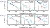 |
Fig. 9 Peak position-velocity (PPV) diagrams of C18O 6–5 (top) and C17O 2–1 (bottom) at i = 45° after convolution with a 0.1″ beam. The red and blue symbols correspond to the red- and blue-shifted velocity components, respectively. The different panels present the PPV for the different simulations. Vertical solid lines show the disk radii extracted for the three models, dashed lines show the steep velocity profile (υ ∝ r-1), and the solid cyan lines indicate the Keplerian curves. The stellar masses are indicated in the top right of each panel. The offset between blue- and red-shifted points are due to the limited spatial and spectral resolution at the high velocities. |
Peak positions are determined for each of the velocity channel maps for each molecular line for the red- and blue-shifted components separately taking channels into account whose peak flux density (Sν in Jy bm-1) is >1% of Smax. They are subsequently rotated according to the direction of the velocity gradient. If an RSD is present, the peak positions of both red- and blue-shifted velocities are expected to follow the Keplerian velocity profile (υ ∝ r-0.5). The combination of infalling rotating envelope and RSD, which exhibits a skewness in the moment one map, is expected to show a steeper velocity profile (υ ∝ r-1) (Yen et al. 2013). However, at high velocities, the peak positions of the red- and blue-shifted velocities can be misaligned on scales of 5 AU owing to the limited spatial resolution. The disk radius is determined by minimizing the difference (~10%) between the best-fit stellar mass inside and at the disk radius.
The peak position-velocity (PPVs) diagrams for C18O 6–5 and C17O 2–1 are shown in Fig. 9. These lines are chosen because they represent two observational extremes in terms of excitation and optical depth. There is a clear distinction between the RSD simulations and a pseudo-disk. The velocity profile of the pseudo-disk is much flatter than expected from an RSD. Thus, spatially and spectrally resolved molecular lines observations can clearly differentiate between an RSD and a pseudo-disk.
All three PPV diagrams indicate a velocity profile close to υ ∝ r-0.5 (for the pseudo-disk see C17O 2–1 PPV in the inner 20 AU). This reflects the fact that the inner 300 AU of the models is dominated by velocity structure that is proportional to r-0.5, which is both the radial velocity  and angular velocity
  (Brinch et al. 2008). From this characterization, the stellar masses can be calculated and indicated in the top righthand corner of Fig. 9. In general, the best-fit stellar masses in the case of RSD are within 30% of the true stellar masses tabulated in Table 1. This is not so for the 2D model in the C18O 6–5 and also C17O 6–5 (not shown) because the inner flattened envelope is warm (>40 K) and dense.
Another parameter that one would like to extract is the disk radius, Rd, which is indicated by the vertical solid line in Fig. 9. The break at Rd is readily seen in the 2D model at ~40 AU for both C18O 6–5 and C17O 2–1. For the case of the 3D MHD simulation (RSD), the best-fit radius varies between 100 and 300 AU. It also exhibits a steep velocity profile (υ ∝ r~−1) at radii >100 AU. The wide range of disk radii is due to the envelope emission dominating the molecular emission because CO is frozen out in the cold part of the disk at those large radii. The issue of disk versus envelope emission becomes apparent in the case of large embedded disk (Rd> 100 AU).
The comparison shows that there is a clear and distinct PPV profile associated with RSD formation from r-0.5 to r-1. A steep velocity profile (υ ∝ r-1) is absent in the pseudo-disk simulation. This seems to indicate that such a steep velocity profile describes ongoing RSD formation based on the given simulations. A pseudo-disk is characterized by a flat velocity profile in the inner regions. Furthermore, the PPV method can simultaneously derive the stellar mass and the extent of the RSD, while separating the infalling rotating envelope from it. For differentiating between RSD and non-RSD, a PPV diagram is a better tool than PV-diagrams.
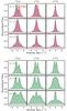 |
Fig. 10 Top: 13CO, C18O, and C17O 3–2 (top), 6–5 (middle), and 9–8 (bottom) spectra at i ~ 0° within a 9″ beam. The blue line shows the synthetic line from simulation with an RSD, while the red line is the simulation without an RSD. Bottom: spectral lines convolved with a 9″ beam simulated from 2D semi-analytical model viewed at face-on orientation. |
4.3. Single-dish line profiles
The previous sections focus on features on small scales, as expected from interferometric observations. The next assessment is to compare the synthetic molecular lines with single-dish observations that probe the physical structure of the large-scale envelope on scales up to a few thousand AU. The image cubes are convolved with three different beams: 9″, 15″, and 20″. These different beams are typical of single-dish CO observations using the JCMT (15″), Atacama Pathfinder EXperiment (APEX, 9″), and Herschel (20″). Figure 10 presents the synthetic CO lines (Ju = 3, 6, and 9) for the two MHD simulations viewed face-on (i ~ 0°) convolved with a 9″ beam. The face-on orientation is considered first to compare with the line profiles in Harsono et al. (2013) for the 2D simulation. The low-lying transitions (Ju = 3) probe the kinematics in the large-scale envelope.
Double-peaked line profiles are present in the 13CO and C18O 3–2 regardless of whether an RSD is present or not. For the 13CO line, an inverse P-Cygni line profile is seen owing to the coherent infalling material onto the disk, while a P-Cygni profile is associated to the pseudo-disk, which is tracing the expanding material due to outflowing material present in the pseudo-disk simulation. Self-absorption causes the double peak in the 13CO 3–2 line due to optical depth (typically, τL> 5) at line center, whereas it is weakly affecting the C18O 3–2 line.
It is interesting to note that there is no significant difference in the J = 6−5 lines between a simulation that forms an RSD as opposed to a pseudo-disk. This transition (Eu ~ 110 K) traces the dense warm gas where a large fraction of the emission comes from ≥40 K gas (Yıldız et al. 2010). The P-Cygni line profile is still visible in the 13CO line, but it is not significant in the C18O line. The lines are also not Gaussian since there are significant wing emission extending up to ± 2 km s-1.
The line profiles for the semi-analytical models within a 9″ beam are shown in the bottom of Fig. 10. They are significantly different from the 3D MHD models, which arises from the prescribed velocity structure. In Harsono et al. (2013), an additional microturbulent broadening of 0.8 km s-1 was added, which results in Gaussian line profiles consistent with the observed single-dish CO line profiles. However, in this paper, we have not included the additional broadening term in order to investigate the emission arising from the true kinematical information. The peaks are more prominent than those in the 3D MHD simulations owing to a jump between the velocity structures of the RSD component and the infalling envelope. In general, the 2D semi-analytical models produce significantly broader lines and significant variations between the CO isotopologs and transitions compared with 3D simulations because of a warmer disk and outflow cavity wall (see Sect. 2.2), which both allow for stronger wing emissions.
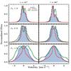 |
Fig. 11 C18O line profiles for the different simulations viewed at i = 45° and i = 90° in the 15″ beam. |
4.3.1. Inclination effects
The simulated lines viewed face-on may not pick up all of the dynamics of the system. Figure 11 shows how the line profiles change with inclination for the three different simulations within a 15″ beam. The lines become broader with increasing inclination because they readily pick up the different velocity components. The Ju = 3 lines exhibit inverse P-Cygni line profiles that are associated with infalling gas. Meanwhile, the higher J transitions show more structured line profiles than do the systems viewed face-on. The C18O 6–5 lines are double-peaked in both cases of RSD formation, while it is single-peaked for the pseudo-disk model. On the other hand, the 9–8 line is significantly broader than the low-J lines reflecting the complexity of the dynamics of the warm dense gas.
4.3.2. Origin of the line broadening
To investigate the source of the line broadening, a set of molecular lines are simulated with zero radial velocity (υr = 0 km s-1) and another with zero azimuthal velocity (υφ = 0 km s-1). For the MHD simulation with RSD, the FWHM value of the C18O 9−8 line decreases to <0.5 km s-1 at all inclinations without any azimuthal velocity component. Such a decrease is not dramatic for face-on orientation; however, it is more than a factor of 3 for intermediate (i ~ 45°) and high inclination (i> 75°) cases. On the other hand, in the case of pseudo-disk formation, both radial and azimuthal velocities are equally important. The origin of the line broadening therefore depends on whether an RSD is forming. If that is indeed the case, the C18O 9–8 is broadened by rotational motions at moderate and high inclinations; at low inclinations, infall dominates the broadening.
FWHM (FWZI as defined at 10% of the peak emission) in km s-1 of the 13CO and C18O lines within a 20″ beam for the MHD simulations viewed at i = 45°.
4.3.3. Line widths and comparison with observation
Molecular line observations are typically characterized by their peak flux densities (or intensities), FWHM, and integrated line flux densities. While the peak flux densities and integrated line fluxes depend on the adopted physical and chemical structure, their FWHM should reflect the general kinematics that are present in the system. In this paper, we focus on the comparison of FWHM and full-width at zero intensity (FWZI) determined at 10% of the peak with observations. A 10% cut-off is chosen since most single-dish observations do not reach higher signal-to-noise, especially for the higher J lines.
These values are calculated for 13CO and C18O lines of the different models from the convolved image cubes. The FWHM and FWZI within a 20″ beam are listed in Table 2 at moderate inclination (i = 45°) to compare the two 3D MHD simulations. Within such a large beam, their values for 13CO and C18O are similar. The FWHM values do not necessarily increase between Ju = 3 and 6, in contrast to the FWZI values (see Fig. 12). This is expected since the wing emissions are much lower than the peak because the emitting region is much smaller than the beam (beam dilution).
Considering all inclinations (0°, 45°, and 90°), the FWHM values of the low-J CO lines are similar between the 3D simulations and 2D semi-analytical models. On the other hand, the line widths of the high-J lines differ significantly. This is expected since most of the 2–1 and 3–2 emission originates in the large-scale envelope, which is similar in terms of kinematics in the three simulations. However, the high-J lines originate in the warm inner regions in which the three simulations show different velocity structures.
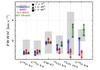 |
Fig. 12 FWHM values of the observed (gray-shaded region) and simulated (symbols) rotational lines of 13CO and C18O as indicated in a 20″ beam. The observed values are taken from Jørgensen et al. (2002), van Kempen et al. (2009a), and San Jose-Garcia et al. (2013). The FWHM of synthetic lines are indicated at specific inclinations as indicated by the symbols: circles for 0°, triangles for 45°, and squares for 90°. The comparison of the FWZI values are specifically for the C18O 3–2 line. The different colors represent the different types of simulations: 3D RSD (RSD), 3D pseudo-disk (no RSD), and 2D semi-analytical model (2D Model). |
Figure 12 presents the comparison between the simulated and observed lines. The observed line widths toward a sample of Class 0 low-mass YSOs are taken from Jørgensen et al. (2002), van Kempen et al. (2009a), and San Jose-Garcia et al. (2013, FWHMN. Sources with known confusion in their line profiles from other nearby sources have been excluded. It is clear that the observed line widths of the low-J lines (Ju = 2 and 3) are significantly greater than the model simulations by a factor of 2. Since these lines probe the large-scale quiescent envelope, the discrepancy between the predicted and observed line widths suggests that the large-scale envelope is turbulent with FWHM ≈ 1 km s-1 or a Doppler b of ~0.4 km s-1, i.e., more than what is included in the current simulations that could be due to an interaction with fast outflow, at least in part. The comparison of the FWZI values also supports this conclusion.
For the dense and warm gas probed by the higher Ju ≥ 6 lines, the predicted line widths are within the observed range for the models that do form an RSD. Moreover, the pseudo-disk (no RSD) simulations predict much smaller line widths than those observed. This line originates in the inner warm parts that are rotationally supported. Our treatment of the inner radius does not affect this since an evacuated cavity is absent in the case of RSD formation. In fact, if an outflow cavity is allowed to form, the 3D RSD predicted line widths would shift upward. Thus, the line width of this particular line reflects the true kinematics in the inner regions. This comparison may suggest that the large observed line widths of C18O 9−8 line indicate that the kinematics of the warm inner envelope are similar to those of a model that forms an RSD. Alternatively, a turbulence with FWHM = 2 km s-1 would be required in the inner parts if RSDs are absent.
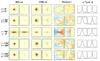 |
Fig. 13 Comparison of synthetic 850 μm, 1100 μm, C18O 2–1 first moment maps and normalized C18O 9–8 spectra for the 3D RSD (left) and pseudo-disk (right) MHD simulations viewed at a few orientations. The images and image cubes are convolved with a 0.1″ beam. The maps sizes are 5″ across similar to Fig. 5. The color scales and line contours are defined in Figs. 5 and 7. The normalized C18O 9–8 spectra refer to a 15″ beam on the same scale as Fig. 11. The inclination (i) and azimuthal angle (φ, rotation angle of the observer around the z axis) are representative only and not exact. |
5. Discussion
5.1. Variations with viewing angles
This paper presents synthetic continuum maps and CO isotopolog lines from 3D MHD simulations and 2D semi-analytical disk formation models out of collapsing rotating envelopes. The aim is to present signatures that can differentiate between embedded rotationally supported disks (RSDs) and a pseudo-disk. Thus far, we have analyzed the continuum and synthetic molecular lines with respect to one viewing angle in the azimuthal direction with φ = 0°. As shown previously by Smith et al. (2012), the line profiles may change with different viewing angles since the collapse process is not spherically symmetric.
To look at the general trend with viewing angles, synthetic images at four different inclinations (i) from 15° to 150° and eight azimuthal angles from 8° to 315° are generated. We have concentrated the analysis on 850 μm, 1100 μm, C18O, and C17O images. Figure 13 presents the continuum and molecular lines at a few viewing angles for the two 3D MHD simulations. The 3D RSD formation predicts an observable spiral feature at near face-on (i ≈ 0°) with high dynamic range (1000). As mentioned earlier, this is due to the infalling material on its way to the disk.
In terms of kinematical signatures, the first moment maps of the C18O 2–1 line are compared for the two cases. Both the RSD and pseudo-disk simulations predict a coherent velocity gradient in the inner 300 AU. However, the velocity gradient is more robust if an RSD is forming. The pseudo-disk simulation shows a velocity gradient in the first moment map that does not necessarily correspond to rotation (see Fig. 1 and Sect. 4.1). Such a direction corresponds to the streamlines of the infalling material from the large-scale envelope to the central star. At high inclinations (i> 75°), this direction of the velocity gradient shifts to east-west direction similar to the RSD simulation, because the first moment map is dominated by the rotational motions that are in the east-west direction.
To assess the general predictions for the large-scale envelope, C18O 9–8 spectra within a 15″ beam are compared. The low-J lines (Ju = 2 and 3) exhibit inverse P-Cygni profiles indicating infalling material in both RSD and pseudo-disk simulations. For the high-J lines, the 3D RSD simulation predicts a broader line than the pseudo-disk simulation in most orientations that are consistent with Fig. 12.
In summary, the results that are presented in previous sections are robust and do not depend on the viewing angles. A pseudo-disk shows more distinct features in the kinematics in the first moment maps that are different from an RSD. A coherent blue- to red-shifted velocity gradient in the inner 1 arcsec aligned with the major axis is most likely a signature of an RSD or of ongoing RSD formation. Although these lines are simulated assuming LTE conditions, non-LTE effects generally decrease the strength of the emission but do not alter the results of the kinematics derived from the molecular limes.
5.2. Masses and sizes
5.2.1. Analysis with continuum
To test models of star and disk formation (e.g., Hueso & Guillot 2005), the flow of mass from envelope to disk to star with time needs to be known. In practice, this means that the masses of the central (proto-)star and of its envelope-disk system need to be inferred from observations and models at different evolutionary stages. A pragmatic way to “extract” the envelope and disk masses is to compare the continuum fluxes within a large beam with those found on “small” scales. Here, the 5″ area is taken because the “small” scale corresponds to 50 kλ at a distance of 140 pc as probed previously with the SMA. Specifically, Jørgensen et al. (2009)2 gives the following formulae:  where fenv is the envelope contribution on “small” scales, S5″ the flux within a 5″ area, S15″ the flux within a 15″ beam, Senv the total envelope flux, and Sdisk the total disk flux. The set of equations above roughly separates the envelope from the disk in terms of continuum flux contribution. There are two issues that need to be addressed in utilizing the equations above: the envelope fraction (fenv) and the “small” scale flux.
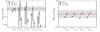 |
Fig. 14 Left: mean deviation of disk masses (gas + dust) derived from 1100 μm continuum and molecular lines fluxes from the true disk mass extracted from the simulations. The gray bars indicate the full range of values for the different orientations. Right: mean deviation of stellar masses measured from molecular lines from the true stellar mass. The colors indicate the different simulations: 3D MHD simulations in blue, 3D MHD pseudo-disk simulation in red, and 2D semi-analytical model in green. The error bars indicate the standard error of the mean. The shaded region shows the area within a factor of 2. |
The first is presented in Sect. 4.1 of Jørgensen et al. (2009). They calculated the envelope contribution as determined from ρdust ∝ r-1.5 spherical envelopes. This yields a maximum contribution of 8% at 850 μm within a scale of 5″ compared with that at 15″. The contribution increases with increasing power-law exponent (16% for ρ ∝ r-1.8). Jørgensen et al. (2009) computed the relative contribution between S50 kλ at 1.1 mm and 15″ in 850 μm. To compute the contributions within the same wavelengths, these values are scaled assuming Fν ∝ ν2.5. In addition, for a given 2D embedded disk model, the projected spherical envelope model is one with an increasing exponent with inclination (i.e., ρ ∝ r-1.8 as i → 90°). In other words, for an embedded YSO viewed at face-on, the best representative spherical model is one with a rather flat density profile. As a result, the envelope contribution from an embedded YSO on small scales changes with inclination.
Another issue is the “small” scale flux at which to determine the envelope contribution. If the size is too small (i.e., 1″), the envelope contribution is naturally negligible, and it is easy to extract the disk flux. However, the disk flux can be underestimated on such a small scale. Furthermore, the flux that is measured at each pixel is always a combination of the envelope and the disk. Thus, it is more intuitive to calculate the envelope’s contribution on scales larger than the disk (~5″, 700 AU at 140 pc) in order to obtain all of the disk’s flux.
For this purpose, following the method in the literature, the envelope and disk masses are determined from comparing the fluxes within a 15″ beam and a 5″ area. This procedure is performed on the images rendered at the 32 different viewing angles, as described in the previous paragraphs. A typical constant envelope fraction of 8% at 850 μm (2% at 1100 μm) is adopted to see how well such a simple estimation based on spherically symmetric envelope model can extract the disk properties of the 2D and 3D simulations.
Once the disk and envelope fluxes at 850 μm have been obtained, the conversion to dust mass follows Jørgensen et al. (2009), Eq. (1), which considers that there is a distribution of temperatures in the envelope set by the luminosity of the protostar. The envelope mass therefore scales both with distance and bolometric luminosity (Lbol). The bolometric luminosities are calculated by constructing the spectral energy distribution at the same viewing angles as the synthetic images. For the disk, a dust temperature of 30 K is adopted to calculate its mass as done in observations. These values are compared to the masses of different components in the simulations (Table 1). The disk mass in the simulation is defined by the velocity structure as described in Sect. 2.3. The leftover material within the computational box is the envelope mass.
Figure 14 presents the ratio of disk masses derived from synthetic continuum observations to the true masses tabulated in Table 1. In the case of the pseudo-disk, the disk mass is taken to be the mass of the region with number densities nH2> 107.5 cm-3. The masses inferred from the continuum fluxes are within a factor of 2 of the true disk mass. There is a small difference in the disk mass between 1100 μm and 850 μm for both 3D RSD and 2D semi-analytical model. Envelope masses agree if scaled to the same 15″ beam.
The spread in the inferred disk masses is greater in the 2D model than in the 3D simulation. The lower end of the spread is occupied by simulations at high inclinations (i> 75°). In such an orientation, the continuum optical depth even at 1100 μm is high since the disk is viewed edge-on and, consequently, a large part of the disk does not contribute to the observable emission. The high end of the spread is when the system is viewed almost face-on where the flattened inner envelope deviates from the spherically symmetric assumption. Finally, the equations above underestimate the disk mass from the 3D simulations because a Tdust = 30 K was assumed to obtain the disk mass, whereas the temperature within the disk is <30 K at large radii. A lower temperature ~10 K would be best for the 3D RSD simulation, while it depends on inclination for the 2D model case.
The results suggest that disk masses can be estimated well from the continuum flux even for the pseudo-disk. However, there is a clear difference in how the disk is defined in all three cases. In the 3D and 2D RSD, the disk mass is defined by its velocity structure such that it is indeed rotationally supported, while the pseudodisk is defined by density. In the latter case, therefore, the difference between the disk and the infalling envelope is not well defined.
In summary, we find that the disk masses as inferred from continuum emission in the 3D simulations and 2D semi-analytical model are within a factor of 2 of the true value. This factor of 2 is due to the viewing angle, and the dust temperature within the disk is lower than the assumed 30 K. However, we find that the pseudo-disk also indicates similar emission on these scales (see also, Chiang et al. 2008). In this case, the disk does not correspond to a Keplerian disk.
5.2.2. Disk radii and stellar masses
Continuum analysis of a large sample of sources yields disk and envelope masses. To fully test the evolutionary models, the stellar masses need to be derived from the kinematics of molecular lines. In addition, the disk radii can be determined from the velocity profiles (see Sect. 4.2) and can also serve as tests for the evolutionary models since disk radius is expected to increase with evolutionary state but to also depend on the initial angular momentum of the core (see Fig. 13 in Harsono et al. 2014). The extent of the RSD is determined from the break in the PPV diagrams (see Fig. 9) for the simulated C18O 2–1, C18O 6–5, C17O 2–1, and C17O 6–5 lines. For the 2D semi-analytical models, the average radius from the four lines is 64 ± 8 AU as derived from the break. For the 3D MHD RSD simulation, the average radius is 230 ± 100 AU. Thus, the inferred drop-off gives a good estimate of the extent of small disks, while a larger disk has a larger error bar associated to it.
Disk masses can also be calculated from the integrated flux densities ( in Jy km s-1) of molecular lines. In this method, the integrated flux densities are extracted within the region defined by the radius in the previous paragraph. The mass calculation is given by (Scoville et al. 1986; Momose et al. 1998; Hogerheijde et al. 1998):
 ![\begin{eqnarray} M_{\rm gas} & = & 5.9 \times 10^{6} \frac{Q(T_{\rm ex})}{ g_{\rm u} A_{\rm ul} \exp{\left (-E_{\rm u} / k_{\rm B} T_{\rm ex} \right ) } } \frac{\mu_{\rm H_2} m_{\rm H_2} }{[X/{\rm H_2}]} \\ \nonumber & & \times \frac{\tau_{\rm L}}{1 - \exp^{-\tau_{\rm L}}} \left ( \frac{d}{\rm 140~pc} \right )^2 \int S_{\upsilon}{\rm d}\upsilon \ M_{\odot}, \end{eqnarray}](/articles/aa/full_html/2015/05/aa24550-14/aa24550-14-eq188.png) (3)where Aul is the Einstein A coefficient of the transition, gu is the degeneracy of the upper level, Eu the upper level energy, Q(Tex) the partition function at an excitation temperature Tex = 40 K, μH2 the mean weight of the gas, [ X/ H2 ] the abundance of molecule X with respect to H2, τL the line optical depth, and kB the Boltzmann constant. A higher excitation temperature for the gas is adopted with respect to the dust temperature following the rotational temperature derived from the observed C18O lines (Yıldız et al. 2013). The derived masses do not depend strongly on the adopted excitation temperature. A constant line optical depth of 0.5 for the C18O and 0.3 for the C17O lines is used, which characterizes the average optical depth over all velocities. The crucial assumption here is the CO abundance, [ X/ H2 ], which is taken to be 10-4, similar to the one in Sect. 2.4. Since the CO abundance will be affected by freeze-out in the cooler parts of the disk, this assumption provides a lower limit to the disk mass.
(3)where Aul is the Einstein A coefficient of the transition, gu is the degeneracy of the upper level, Eu the upper level energy, Q(Tex) the partition function at an excitation temperature Tex = 40 K, μH2 the mean weight of the gas, [ X/ H2 ] the abundance of molecule X with respect to H2, τL the line optical depth, and kB the Boltzmann constant. A higher excitation temperature for the gas is adopted with respect to the dust temperature following the rotational temperature derived from the observed C18O lines (Yıldız et al. 2013). The derived masses do not depend strongly on the adopted excitation temperature. A constant line optical depth of 0.5 for the C18O and 0.3 for the C17O lines is used, which characterizes the average optical depth over all velocities. The crucial assumption here is the CO abundance, [ X/ H2 ], which is taken to be 10-4, similar to the one in Sect. 2.4. Since the CO abundance will be affected by freeze-out in the cooler parts of the disk, this assumption provides a lower limit to the disk mass.
Figure 14 presents the masses obtained from the integrated line-flux densities. They show a much larger scatter than the masses obtained from the dust continuum flux. The symbols indicate the values appropriate for masses derived at moderate inclinations. For the case of RSD formation, the low-end of the spread is due to near face-on orientation (30°>i> 150°) in which the obtained disk sizes are half of the true RSD, and consequently, the disk mass is lower than average. In the 2D semi-analytical model case, the physical structure of the inner envelope plays a role. The conversion between integrated flux to mass also assumes that the emission at all velocities is dominated by the disk, which is only true for emission at the wings (high velocities ≳1 km s-1). However, in the 2D semi-analytical model, the inner envelope is highly flattened compared to that of the 3D MHD simulation such that high density gas (nH2> 106 cm-3) surrounds the RSD (see Fig. 1). The disk therefore does not dominate the integrated flux density at this particular time (see Fig. 8 of Harsono et al. 2013), so that the integrated flux density is not correlated to its mass. As a result, a good estimate of the disk’s molecular mass can only be obtained if the system is oriented at moderate inclinations and the RSD is assumed to dominate the molecular emission at all velocities.
The disk masses derived from the 2–1 line are generally higher than that from the 6–5 line. Since the RSD obtained from the 6–5 emission is smaller than for the 2–1 line (e.g., 200 vs. 100 AU), the integrated line flux density is extracted from a smaller region, which results in a much lower mass. The size of the RSD revealed by the 6–5 line is generally smaller than the size revealed by the 2–1 line. This is because the 6–5 line emission arises from the dense warm regions in the vicinity of the protostar. As a result of the smaller size, the mass is also lower than the one derived from the 2–1 line. The masses obtained from the integrated 2–1 line are better estimates of the true disk mass.
The 3D MHD and 2D semi-analytical RSD formation predict the same behavior in terms of disk masses in both C17O and C18O lines. The difference of the masses obtained in the 2–1 and the 6–5 lines are also similar for the two isotopologs. The 2D semi-analytical model predicts a smaller spread than the 3D RSD model in the disk masses obtained from the C17O 2−1 line since the high-density region is more compact in the 2D case, and therefore, the C17O 2–1 integrated flux density obtained in the 2D model does not vary as much as in the 3D simulation. The comparison between the 2D semi-analytical model and 3D MHD shows that the reliability of the observables for tracing the true masses depends on the physical structure of the inner envelope.
The stellar masses obtained from the PPV method are shown in Fig. 14. They are typically within a factor of 2 of the true stellar masses. The best-fit values for synthetic molecular lines viewed at i< 15° tend to be more than twice the true stellar mass. This is due to the difficulties obtaining the peak positions at high velocities since they are most likely to be below the noise level. The 2D semi-analytical model indicates better agreement with true stellar masses than those of the 3D model because their velocity structures are different. The kinematics of the envelope is the same at all viewing angles in 2D. However, there are lines of sight that pick up significant sub-Keplerian gas infalling onto the disk in 3D as shown in Fig. 3. Therefore, stellar masses as obtained from spatially and spectrally resolved molecular observations are good estimates of the true stellar mass within a factor of 2, which is less than the uncertainty in the inclination.
From the analysis of the synthetic observations, spatially (≲0.1″ at 140 pc) and spectrally (≤0.1 km s-1) resolved optically thin molecular lines at two energy levels (e.g., 2–1 and 6–5) are required to understand the physical structure of the inner envelope. The disk masses obtained from the two lines are similar in the pseudodisk case, while they can differ by an order of magnitude in RSD case. The simple PPV analysis directly from the data can already differentiate between the RSD and a pseudo-disk. However, sophisticated modeling tools are needed to infer the physical structure of the disk.
6. Summary and conclusions
We have presented the observables in continuum and molecular lines for the two 3D MHD simulations of Li et al. (2013) and 2D semi-analytical models of collapse and disk formation. Snapshots of two different MHD simulations of a relatively weakly magnetized core (B0 = 11μG) at the same time after the onset of collapse are used. One simulation has an initial magnetic field axis aligned with the rotation axis in which a rotational supported disk (RSD) does not form, but a pseudo-disk and outflowing gas are present. The other MHD simulation starts with the magnetic field axis oriented perpendicular to the rotation axis, which results in the formation of an RSD (see Figs. 1 and 3). These simulations explore the two extremes of the magnetic field orientation. The synthetic observables are then compared to a 2D semi-analytical model without magnetic field (Visser et al. 2009) with similar initial conditions (1 M⊙ and Ω0 = 10-13 Hz). Accurate dust temperatures are calculated using the 3D continuum radiative transfer tool RADMC3D with the same dust opacities and central temperature for all three models. Continuum images and thermalized CO molecular lines are produced using the same radiative transfer code and method. Freeze-out of CO onto dust grains is included. This paper focuses on presenting similarities and differences in the predicted observables. The main results and conclusions are as follows.
-
Synthetic continuum images of the two MHD simulations and 2D semi-analytical model indicate that a spatial resolution of 14 AU and high dynamic range (1000) are required to differentiate between disk formation scenarios. Furthermore, the features that are present during the collapse are more easily observed in the 450 μm continuum images than at longer wavelengths. It is difficult to test disk formation models toward highly inclined systems using continuum data since both RSD and pseudo-disk formation show similar elongated features.
-
The kinematical structures as revealed by the first moment maps of the synthetic molecular lines show a coherent blue- to red-shifted velocity gradient for both RSD models and for the pseudo-disk in the inner ~300 AU. However, the pseudo-disk shows a velocity gradient in the north-south direction, while the RSD shows an east-west gradient similar to the orientation of the flattened structure in the model. Moreover, the RSD formation in both 3D and 2D exhibits skewness in their first moment maps caused by the infalling rotating envelope component on larger scales, which is absent in the case of the pseudo-disk. The velocity gradient in the case of the pseudo-disk is a nearly straight line from the star to the large-scale structure, since it is tracing the streams of material directly from the envelope onto the star. Thus, one can readily mistake a pseudo-disk for an RSD unless one performs additional analysis, such as the peak position diagrams.
-
Position-velocity (PV) diagrams constructed from C18O and C17O image cubes predict rotational signatures in both pseudo-disk and RSD formation, which is seen most prominently in C17O data. This is due to the strength of rotation in the inner regions for both simulations. A combination of C18O and C17O lines is required to disentangle the RSD from a pseudo-disk. The signatures of infalling material in the pseudo-disk simulation are stronger in the C18O lines. The velocity structure constructed from the peak position-velocity (PPV) diagrams are used to differentiate between the pseudo-disk and the RSD. Velocity structures described by υ ∝ r-0.5 and υ ∝ r-1 are present in both cases of RSD formation, whereas a flatter velocity profile is seen in the pseudo-disk case. We find that this conclusion is robust for different inclinations and rotations.
-
The image cubes are convolved with large beams (≥9″) to simulate single-dish observations probing the large-scale envelope. The C18O 2–1 and 3–2 line widths are similar between the three simulations with FWHM ~ 1 km s-1or Doppler b of 0.4 km s-1. This is because the emitting regions in the large-scale envelopes are similar. The observed FWHM values are higher than in those predicted from the simulations by a factor of 2. This suggests that the large-scale envelopes of low-mass embedded YSOs are significantly more turbulent than these models, which may be due to an interaction with a fast outflow (San Jose-Garcia et al. 2013).
-
The comparison of the high-J lines (13CO 6–5, 13CO 10−9, and C18O 9–8) indicates that the current simulations with RSD formation can reproduce the observed line widths solely due to the rotation + infall motions. On the other hand, the predicted line widths from the pseudo-disk are significantly smaller than the observed values. The mechanism(s) that are responsible for broadening the 6–5 and 9–8 lines thus depend on the whether or not an RSD is present. If no RSD is present, the observations would imply an increasing level of turbulence with decreasing radii; if an RSD is present, turbulence would not be needed, although it can still be present in the disk at some level.
-
Masses derived from continuum and molecular lines from simulations and analyzed in the same way as observations depend on the physical structure on small scales. The disk masses obtained from the continuum flux in small beams (a few ″) generally agree with the true disk mass. Disk masses obtained from the integrated molecular line flux depend strongly on the physical structure. If the disk is small and cold compared to the flattened inner envelope, inferred masses can be lower by an order of magnitude from the true disk mass since the disk does not contribute to the integrated line flux density. However, if the disk is large and warm enough to prevent significant freeze-out, the mass obtained from the low-J lines can give a good estimate of the true RSD mass provided that the system is inclined toward us. Both the stellar masses and disk-to-envelope mass ratios are within a factor of 2 of the true masses. The presence of the RSD cannot be determined solely from continuum data alone, however the continuum flux provides a good estimate of the mass on small scales. Multiple spectrally and spatially resolved molecular line observations are needed to confirm the presence of RSD.

Acknowledgments
We thank Atilla Juhász for providing scripts for generating and analyzing RADMC3D input and output files. We also thank Kees Dullemond for providing RADMC3D. We are grateful to Michiel Hogerheijde, Floris van der Tak, and Lee Hartmann for commenting on the manuscript. We thank the anonymous referee for the useful comments that have improved this manuscript. This work is supported by The Netherlands Research School for Astronomy (NOVA). Astrochemistry in Leiden is supported by the Netherlands Research School for Astronomy (NOVA), by a Royal Netherlands Academy of Arts and Sciences (KNAW) professor prize, and by the European Union A-ERC grant 291141 CHEMPLAN. Z.Y.L. is supported in part by NASA 10AH30G, NNX14B38G, and NSF AST1313083.
References
- Belloche, A. 2013, in EAS Pub. Ser., 62, 25 [Google Scholar]
- Bodenheimer, P. 1995, ARA&A, 33, 199 [NASA ADS] [CrossRef] [Google Scholar]
- Brinch, C., Crapsi, A., Hogerheijde, M. R., & Jørgensen, J. K. 2007, A&A, 461, 1037 [NASA ADS] [CrossRef] [EDP Sciences] [Google Scholar]
- Brinch, C., Hogerheijde, M. R., & Richling, S. 2008, A&A, 489, 607 [NASA ADS] [CrossRef] [EDP Sciences] [Google Scholar]
- Cassen, P., & Moosman, A. 1981, Icarus, 48, 353 [NASA ADS] [CrossRef] [Google Scholar]
- Chiang, H.-F., Looney, L. W., Tassis, K., Mundy, L. G., & Mouschovias, T. C. 2008, ApJ, 680, 474 [NASA ADS] [CrossRef] [Google Scholar]
- Commerçon, B., Launhardt, R., Dullemond, C., & Henning, T. 2012a, A&A, 545, A98 [NASA ADS] [CrossRef] [EDP Sciences] [Google Scholar]
- Commerçon, B., Levrier, F., Maury, A. J., Henning, T., & Launhardt, R. 2012b, A&A, 548, A39 [NASA ADS] [CrossRef] [EDP Sciences] [Google Scholar]
- Crapsi, A., van Dishoeck, E. F., Hogerheijde, M. R., Pontoppidan, K. M., & Dullemond, C. P. 2008, A&A, 486, 245 [NASA ADS] [CrossRef] [EDP Sciences] [Google Scholar]
- Crutcher, R. M. 2012, ARA&A, 50, 29 [NASA ADS] [CrossRef] [Google Scholar]
- de Graauw, T., Helmich, F. P., Phillips, T. G., et al. 2010, A&A, 518, L6 [NASA ADS] [CrossRef] [EDP Sciences] [Google Scholar]
- Doty, S. D., van Dishoeck, E. F., van der Tak, F. F. S., & Boonman, A. M. S. 2002, A&A, 389, 446 [NASA ADS] [CrossRef] [EDP Sciences] [Google Scholar]
- Doty, S. D., Schöier, F. L., & van Dishoeck, E. F. 2004, A&A, 418, 1021 [NASA ADS] [CrossRef] [EDP Sciences] [Google Scholar]
- Dunham, M. M., & Vorobyov, E. I. 2012, ApJ, 747, 52 [NASA ADS] [CrossRef] [Google Scholar]
- Dunham, M. M., Evans, II, N. J., Terebey, S., Dullemond, C. P., & Young, C. H. 2010, ApJ, 710, 470 [NASA ADS] [CrossRef] [Google Scholar]
- Dunham, M. M., Stutz, A. M., Allen, L. E., et al. 2014, in Protostars and Planets VI, eds. H. Beuther, C. Dullemond, & T. Henning (Tucson: Univ. of Arizona Press), 195 [Google Scholar]
- Enoch, M. L., Corder, S., Duchêne, G., et al. 2011, ApJS, 195, 21 [NASA ADS] [CrossRef] [Google Scholar]
- Galli, D., & Shu, F. H. 1993, ApJ, 417, 220 [NASA ADS] [CrossRef] [Google Scholar]
- Galli, D., Lizano, S., Shu, F. H., & Allen, A. 2006, ApJ, 647, 374 [NASA ADS] [CrossRef] [Google Scholar]
- Harsono, D., Visser, R., Bruderer, S., van Dishoeck, E. F., & Kristensen, L. E. 2013, A&A, 555, A45 [NASA ADS] [CrossRef] [EDP Sciences] [Google Scholar]
- Harsono, D., Jørgensen, J. K., van Dishoeck, E. F., et al. 2014, A&A, 562, A77 [NASA ADS] [CrossRef] [EDP Sciences] [Google Scholar]
- Hennebelle, P., & Ciardi, A. 2009, A&A, 506, L29 [NASA ADS] [CrossRef] [EDP Sciences] [Google Scholar]
- Hogerheijde, M. R., van Dishoeck, E. F., Blake, G. A., & van Langevelde, H. J. 1998, ApJ, 502, 315 [NASA ADS] [CrossRef] [PubMed] [Google Scholar]
- Hueso, R., & Guillot, T. 2005, A&A, 442, 703 [NASA ADS] [CrossRef] [EDP Sciences] [Google Scholar]
- Joos, M., Hennebelle, P., & Ciardi, A. 2012, A&A, 543, A128 [NASA ADS] [CrossRef] [EDP Sciences] [Google Scholar]
- Joos, M., Hennebelle, P., Ciardi, A., & Fromang, S. 2013, A&A, 554, A17 [NASA ADS] [CrossRef] [EDP Sciences] [Google Scholar]
- Jørgensen, J. K., Schöier, F. L., & van Dishoeck, E. F. 2002, A&A, 389, 908 [NASA ADS] [CrossRef] [EDP Sciences] [Google Scholar]
- Jørgensen, J. K., Schöier, F. L., & van Dishoeck, E. F. 2005, A&A, 435, 177 [NASA ADS] [CrossRef] [EDP Sciences] [Google Scholar]
- Jørgensen, J. K., van Dishoeck, E. F., Visser, R., et al. 2009, A&A, 507, 861 [NASA ADS] [CrossRef] [EDP Sciences] [Google Scholar]
- Keene, J., & Masson, C. R. 1990, ApJ, 355, 635 [NASA ADS] [CrossRef] [Google Scholar]
- Kristensen, L. E., van Dishoeck, E. F., Benz, A. O., et al. 2013, A&A, 557, A23 [NASA ADS] [CrossRef] [EDP Sciences] [Google Scholar]
- Krumholz, M. R., Crutcher, R. M., & Hull, C. L. H. 2013, ApJ, 767, L11 [NASA ADS] [CrossRef] [Google Scholar]
- Li, Z.-Y., Krasnopolsky, R., & Shang, H. 2011, ApJ, 738, 180 [NASA ADS] [CrossRef] [Google Scholar]
- Li, Z.-Y., Krasnopolsky, R., & Shang, H. 2013, ApJ, 774, 82 [NASA ADS] [CrossRef] [Google Scholar]
- Li, Z.-Y., Banerjee, R., Pudritz, R. E., et al. 2014a, in Protostars and Planets VI, eds. H. Beuther, C. Dullemond, & T. Henning (Tucson: Univ. of Arizona Press), 173 [Google Scholar]
- Li, Z.-Y., Krasnopolsky, R., Shang, H., & Zhao, B. 2014b, ApJ, in press [Google Scholar]
- Lin, D. N. C., & Pringle, J. E. 1990, ApJ, 358, 515 [NASA ADS] [CrossRef] [Google Scholar]
- Lommen, D., Jørgensen, J. K., van Dishoeck, E. F., & Crapsi, A. 2008, A&A, 481, 141 [NASA ADS] [CrossRef] [EDP Sciences] [Google Scholar]
- Looney, L. W., Mundy, L. G., & Welch, W. J. 2003, ApJ, 592, 255 [NASA ADS] [CrossRef] [Google Scholar]
- Lynden-Bell, D., & Pringle, J. E. 1974, MNRAS, 168, 603 [NASA ADS] [CrossRef] [Google Scholar]
- Machida, M. N., & Matsumoto, T. 2011, MNRAS, 413, 2767 [NASA ADS] [CrossRef] [Google Scholar]
- Momose, M., Ohashi, N., Kawabe, R., Nakano, T., & Hayashi, M. 1998, ApJ, 504, 314 [NASA ADS] [CrossRef] [Google Scholar]
- Myers, A. T., McKee, C. F., Cunningham, A. J., Klein, R. I., & Krumholz, M. R. 2013, ApJ, 766, 97 [NASA ADS] [CrossRef] [Google Scholar]
- Ohashi, N., Hayashi, M., Ho, P. T. P., & Momose, M. 1997, ApJ, 475, 211 [Google Scholar]
- Robitaille, T. P., Whitney, B. A., Indebetouw, R., Wood, K., & Denzmore, P. 2006, ApJS, 167, 256 [NASA ADS] [CrossRef] [Google Scholar]
- Rothman, L., Gordon, I., Barbe, A., et al. 2009, J. Quant. Spectr. Rad. Transf., 110, 533 [NASA ADS] [CrossRef] [Google Scholar]
- San Jose-Garcia, I., Mottram, J. C., Kristensen, L. E., & van Dishoeck, E. F., et al. 2013, A&A, 553, A125 [NASA ADS] [CrossRef] [EDP Sciences] [Google Scholar]
- Santos-Lima, R., de Gouveia Dal Pino, E. M., & Lazarian, A. 2012, ApJ, 747, 21 [NASA ADS] [CrossRef] [Google Scholar]
- Sargent, A. I., & Beckwith, S. 1987, ApJ, 323, 294 [NASA ADS] [CrossRef] [Google Scholar]
- Schöier, F. L., van der Tak, F. F. S., van Dishoeck, E. F., & Black, J. H. 2005, A&A, 432, 369 [NASA ADS] [CrossRef] [EDP Sciences] [Google Scholar]
- Scoville, N. Z., Sargent, A. I., Sanders, D. B., et al. 1986, ApJ, 303, 416 [NASA ADS] [CrossRef] [Google Scholar]
- Seifried, D., Banerjee, R., Pudritz, R. E., & Klessen, R. S. 2012, MNRAS, 423, L40 [Google Scholar]
- Shakura, N. I., & Sunyaev, R. A. 1973, A&A, 24, 337 [NASA ADS] [Google Scholar]
- Smith, R. J., Shetty, R., Stutz, A. M., & Klessen, R. S. 2012, ApJ, 750, 64 [NASA ADS] [CrossRef] [Google Scholar]
- Takakuwa, S., Saito, M., Lim, J., et al. 2012, ApJ, 754, 52 [NASA ADS] [CrossRef] [Google Scholar]
- Terebey, S., Shu, F. H., & Cassen, P. 1984, ApJ, 286, 529 [NASA ADS] [CrossRef] [Google Scholar]
- Terebey, S., Chandler, C. J., & Andre, P. 1993, ApJ, 414, 759 [NASA ADS] [CrossRef] [Google Scholar]
- Tobin, J. J., Hartmann, L., Chiang, H.-F., et al. 2012, Nature, 492, 83 [NASA ADS] [CrossRef] [PubMed] [Google Scholar]
- van Kempen, T. A., van Dishoeck, E. F., Güsten, R., et al. 2009a, A&A, 507, 1425 [NASA ADS] [CrossRef] [EDP Sciences] [Google Scholar]
- van Kempen, T. A., van Dishoeck, E. F., Hogerheijde, M. R., & Güsten, R. 2009b, A&A, 508, 259 [Google Scholar]
- Visser, R., & Dullemond, C. P. 2010, A&A, 519, A28 [NASA ADS] [CrossRef] [EDP Sciences] [Google Scholar]
- Visser, R., van Dishoeck, E. F., Doty, S. D., & Dullemond, C. P. 2009, A&A, 495, 881 [NASA ADS] [CrossRef] [EDP Sciences] [Google Scholar]
- Vorobyov, E. I., Zakhozhay, O. V., & Dunham, M. M. 2013, MNRAS, 433, 3256 [NASA ADS] [CrossRef] [Google Scholar]
- Wilson, T. L., & Rood, R. 1994, ARA&A, 32, 191 [NASA ADS] [CrossRef] [Google Scholar]
- Yen, H.-W., Takakuwa, S., Ohashi, N., & Ho, P. T. P. 2013, ApJ, 772, 22 [NASA ADS] [CrossRef] [Google Scholar]
- Yıldız, U. A., van Dishoeck, E. F., Kristensen, L. E., et al. 2010, A&A, 521, L40 [Google Scholar]
- Yıldız, U. A., Kristensen, L. E., van Dishoeck, E. F., et al. 2013, A&A, 556, A89 [NASA ADS] [CrossRef] [EDP Sciences] [Google Scholar]
- Young, C. H., & Evans, II, N. J. 2005, ApJ, 627, 293 [NASA ADS] [CrossRef] [Google Scholar]
All Tables
FWHM (FWZI as defined at 10% of the peak emission) in km s-1 of the 13CO and C18O lines within a 20″ beam for the MHD simulations viewed at i = 45°.
All Figures
|
Fig. 1 Density and dust temperature structures in the inner 200 AU radius for all three simulations at t ~ 1.2 × 10⁵ years. Temperature contours at 25 K and 40 K are indicated in the right panels. Top: a vertical slice (R − z slice at φ = 0 where R denotes the cylindrical radial coordinate) of the 3D MHD simulation of RSD formation. Middle: a vertical slice of the 3D MHD simulation of a pseudo-disk (no RSD). Bottom: 2D semi-analytical disk formation model. The red lines highlight the region of the stable RSD. |
| In the text | |
|
Fig. 2 Velocity streamlines for the two MHD simulations in Li et al. (2013). The simulations are rendered with paraview (http://www.paraview.org). Left: 3D MHD simulation of a collapsing uniform sphere with the magnetic field vector perpendicular to the rotation axis. Right: The simulation with magnetic field vector aligned with the rotation axis. The color of the arrows indicate the azimuthal velocity vector, υφ, in km s-1. The solid black arrows indicate the general stream lines in the two simulations. The dark shaded colors indicate the density isocontours of nH2 = 107.5 cm-3 up to 1010.5 cm-3 (red). |
| In the text | |
|
Fig. 3 Radial (solid) and azimuthal velocities (dashed) at the midplane (θ = π/ 2, φ = 0) for the three different models: 3D RSD MHD simulation (blue), 3D no RSD (red), and 2D model (green). |
| In the text | |
|
Fig. 4 Continuum intensity maps of 450, 850, 1100, and 1300 μm for the MHD disk formation simulation (left panels) and pseudo-disk (no RSD, right panels) at i = 45° at 5 AU pixels. Note the high dynamic range needed to see all of the structures. |
| In the text | |
|
Fig. 5 Convolved continuum maps in the inner 5″ of 450 (left) and 1100 (right) μm at i = 45°. The images are convolved with 1″, 0.5″, and 0.1″ beams as indicated in each panel. For each panel, the top row shows synthetic image of RSD simulation and the pseudo-disk simulation is shown in the bottom row. The color scale presents the full range of the emission above 10-2 mJy/bm, not all of which may be detectable. Solid red contours are drawn from 3σ up to maximum at 6 logarithmic steps where 1σ is 0.01 × the maximum (dynamical range of 100) with a minimum at 0.5 mJy/bm for the 1″ and 0.5″ images. For the images convolved with a 0.1″ beam, the red contours are drawn with a minimum noise level of 0.5 mJy/bm for 450 μm and 0.05 mJy/bm at longer wavelengths with a dynamic range of 1000, as appropriate for the full ALMA. |
| In the text | |
|
Fig. 6 Synthetic 850 μm continuum images convolved with 0.5″ (top) and 0.1″ (bottom) beams for the three simulations viewed at 90° (edge-on): RSD formation (left), pseudo-disk (center), and 2D semi-analytical model (right). The red solid lines are drawn at the same contours as in Fig. 5. |
| In the text | |
|
Fig. 7 First moment maps of C18O 2–1 (top) and 6–5 (bottom) for the three simulations viewed i = 45° convolved with a 0.1″ beam. The solid line shows the 20% intensity contour of the moment zero ( |
| In the text | |
|
Fig. 8 PV maps of C18O (left) and C17O (right) along the velocity gradients as seen in Fig. 7 for an inclination of 45° and 0.1″ beam. The top panels show the J = 2–1 line and the bottom panels show the 6–5 transition. The blue rectangle indicates the radii of RSDs. The dashed lines indicate the inclination corrected Keplerian curves associated to the stellar mass. The red color scales show emission from 10% to the peak intensity. |
| In the text | |
|
Fig. 9 Peak position-velocity (PPV) diagrams of C18O 6–5 (top) and C17O 2–1 (bottom) at i = 45° after convolution with a 0.1″ beam. The red and blue symbols correspond to the red- and blue-shifted velocity components, respectively. The different panels present the PPV for the different simulations. Vertical solid lines show the disk radii extracted for the three models, dashed lines show the steep velocity profile (υ ∝ r-1), and the solid cyan lines indicate the Keplerian curves. The stellar masses are indicated in the top right of each panel. The offset between blue- and red-shifted points are due to the limited spatial and spectral resolution at the high velocities. |
| In the text | |
|
Fig. 10 Top: 13CO, C18O, and C17O 3–2 (top), 6–5 (middle), and 9–8 (bottom) spectra at i ~ 0° within a 9″ beam. The blue line shows the synthetic line from simulation with an RSD, while the red line is the simulation without an RSD. Bottom: spectral lines convolved with a 9″ beam simulated from 2D semi-analytical model viewed at face-on orientation. |
| In the text | |
|
Fig. 11 C18O line profiles for the different simulations viewed at i = 45° and i = 90° in the 15″ beam. |
| In the text | |
|
Fig. 12 FWHM values of the observed (gray-shaded region) and simulated (symbols) rotational lines of 13CO and C18O as indicated in a 20″ beam. The observed values are taken from Jørgensen et al. (2002), van Kempen et al. (2009a), and San Jose-Garcia et al. (2013). The FWHM of synthetic lines are indicated at specific inclinations as indicated by the symbols: circles for 0°, triangles for 45°, and squares for 90°. The comparison of the FWZI values are specifically for the C18O 3–2 line. The different colors represent the different types of simulations: 3D RSD (RSD), 3D pseudo-disk (no RSD), and 2D semi-analytical model (2D Model). |
| In the text | |
|
Fig. 13 Comparison of synthetic 850 μm, 1100 μm, C18O 2–1 first moment maps and normalized C18O 9–8 spectra for the 3D RSD (left) and pseudo-disk (right) MHD simulations viewed at a few orientations. The images and image cubes are convolved with a 0.1″ beam. The maps sizes are 5″ across similar to Fig. 5. The color scales and line contours are defined in Figs. 5 and 7. The normalized C18O 9–8 spectra refer to a 15″ beam on the same scale as Fig. 11. The inclination (i) and azimuthal angle (φ, rotation angle of the observer around the z axis) are representative only and not exact. |
| In the text | |
|
Fig. 14 Left: mean deviation of disk masses (gas + dust) derived from 1100 μm continuum and molecular lines fluxes from the true disk mass extracted from the simulations. The gray bars indicate the full range of values for the different orientations. Right: mean deviation of stellar masses measured from molecular lines from the true stellar mass. The colors indicate the different simulations: 3D MHD simulations in blue, 3D MHD pseudo-disk simulation in red, and 2D semi-analytical model in green. The error bars indicate the standard error of the mean. The shaded region shows the area within a factor of 2. |
| In the text | |
Current usage metrics show cumulative count of Article Views (full-text article views including HTML views, PDF and ePub downloads, according to the available data) and Abstracts Views on Vision4Press platform.
Data correspond to usage on the plateform after 2015. The current usage metrics is available 48-96 hours after online publication and is updated daily on week days.
Initial download of the metrics may take a while.