| Issue |
A&A
Volume 576, April 2015
|
|
|---|---|---|
| Article Number | A107 | |
| Number of page(s) | 25 | |
| Section | Interstellar and circumstellar matter | |
| DOI | https://doi.org/10.1051/0004-6361/201424088 | |
| Published online | 13 April 2015 | |
Planck intermediate results. XXII. Frequency dependence of thermal emission from Galactic dust in intensity and polarization⋆
1
APC, AstroParticule et Cosmologie, Université Paris Diderot,
CNRS/IN2P3, CEA/lrfu, Observatoire de Paris, Sorbonne Paris Cité,
10 rue Alice Domon et Léonie
Duquet, 75205
Paris Cedex 13,
France
2
African Institute for Mathematical Sciences,
6–8 Melrose Road, Muizenberg,
Cape Town, South
Africa
3
Agenzia Spaziale Italiana Science Data Center,
via del Politecnico snc,
00133, Roma, Italy
4
Agenzia Spaziale Italiana, Viale Liegi 26, Roma, Italy
5
Astrophysics Group, Cavendish Laboratory, University of
Cambridge, J J Thomson
Avenue, Cambridge
CB3 0HE,
UK
6
Astrophysics & Cosmology Research Unit, School of Mathematics,
Statistics & Computer Science, University of KwaZulu-Natal,
Westville Campus, Private Bag
X54001, 4000
Durban, South
Africa
7
Atacama Large Millimeter/submillimeter Array, ALMA Santiago
Central Offices, Alonso de Cordova
3107, Vitacura, Casilla
763 0355
Santiago,
Chile
8
CITA, University of Toronto, 60 St. George St., Toronto, ON
M5S 3H8,
Canada
9
CNR – ISTI, Area della Ricerca, via G. Moruzzi 1, Pisa, Italy
10
CNRS, IRAP, 9
Av. colonel Roche, BP
44346, 31028
Toulouse Cedex 4,
France
11
California Institute of Technology, Pasadena, California, USA
12
Centro de Estudios de Física del Cosmos de Aragón
(CEFCA), Plaza San Juan, 1, planta
2, 44001
Teruel,
Spain
13
Computational Cosmology Center, Lawrence Berkeley National
Laboratory, Berkeley,
California,
USA
14
DSM/Irfu/SPP, CEA-Saclay, 91191
Gif-sur-Yvette Cedex,
France
15
DTU Space, National Space Institute, Technical University of
Denmark, Elektrovej
327, 2800
Kgs. Lyngby,
Denmark
16
Département de Physique Théorique, Université de
Genève, 24 quai E.
Ansermet, 1211
Genève 4,
Switzerland
17
Departamento de Física Fundamental, Facultad de Ciencias,
Universidad de Salamanca, 37008
Salamanca,
Spain
18 Departamento de Física, Universidad
de Oviedo, Avda. Calvo Sotelo
s/n, Oviedo,
Spain
19
Department of Astronomy and Astrophysics, University of
Toronto, 50 Saint George Street,
Toronto, Ontario,
Canada
20
Department of Astrophysics/IMAPP, Radboud University
Nijmegen, PO Box
9010, 6500 GL
Nijmegen, The
Netherlands
21
Department of Physics & Astronomy, University of British
Columbia, 6224 Agricultural Road,
Vancouver, British
Columbia, Canada
22
Department of Physics and Astronomy, Dana and David Dornsife
College of Letter, Arts and Sciences, University of Southern California,
Los Angeles, CA
90089,
USA
23
Department of Physics and Astronomy, University College
London, London
WC1E 6BT,
UK
24
Department of Physics, Gustaf Hällströmin katu 2a, University of
Helsinki, Helsinki,
Finland
25
Department of Physics, Princeton University,
Princeton, New Jersey, USA
26
Department of Physics, University of California,
Santa Barbara, California, USA
27
Department of Physics, University of Illinois at
Urbana-Champaign, 1110 West Green
Street, Urbana,
Illinois,
USA
28
Dipartimento di Fisica e Astronomia G. Galilei, Università degli
Studi di Padova, via Marzolo
8, 35131
Padova,
Italy
29
Dipartimento di Fisica e Scienze della Terra, Università di
Ferrara, via Saragat
1, 44122
Ferrara,
Italy
30
Dipartimento di Fisica, Università La Sapienza,
P. le A. Moro 2, Roma, Italy
31
Dipartimento di Fisica, Università degli Studi di
Milano, via Celoria,
16, Milano,
Italy
32
Dipartimento di Fisica, Università degli Studi di
Trieste, via A. Valerio
2, Trieste,
Italy
33
Dipartimento di Fisica, Università di Roma Tor
Vergata, via della Ricerca
Scientifica, 1
Roma,
Italy
34
Discovery Center, Niels Bohr Institute,
Blegdamsvej 17, Copenhagen, Denmark
35
Dpto. Astrofísica, Universidad de La Laguna (ULL),
38206, La Laguna, Tenerife,
Spain
36
European Southern Observatory, ESO Vitacura, Alonso de Cordova
3107, Vitacura,
Casilla
19001
Santiago,
Chile
37
European Space Agency, ESAC, Planck Science Office, Camino bajo
del Castillo, s/n, Urbanización
Villafranca del Castillo, Villanueva de la Cañada, Madrid, Spain
38
European Space Agency, ESTEC, Keplerlaan 1, 2201 AZ
Noordwijk, The
Netherlands
39
Helsinki Institute of Physics, Gustaf Hällströmin katu 2,
University of Helsinki, Helsinki, Finland
40
INAF–Osservatorio Astronomico di Padova,
Vicolo dell’Osservatorio 5,
Padova,
Italy
41
INAF–Osservatorio Astronomico di Roma,
via di Frascati 33,
Monte Porzio Catone,
Italy
42
INAF–Osservatorio Astronomico di Trieste,
via G.B. Tiepolo 11,
Trieste,
Italy
43
INAF/IASF Bologna, via Gobetti, 101, Bologna, Italy
44
INAF/IASF Milano, via E. Bassini 15, Milano, Italy
45
INFN, Sezione di Bologna, via Irnerio 46, 40126
Bologna,
Italy
46
INFN, Sezione di Roma 1, Università di Roma
Sapienza, P.le Aldo Moro
2, 00185,
Roma,
Italy
47
INFN/National Institute for Nuclear Physics,
via Valerio 2, 34127
Trieste,
Italy
48
IPAG: Institut de Planétologie et d’Astrophysique de Grenoble,
Université Joseph Fourier, Grenoble 1/CNRS-INSU, UMR 5274,
38041
Grenoble,
France
49
Imperial College London, Astrophysics group, Blackett
Laboratory, Prince Consort
Road, London,
SW7 2AZ,
UK
50
Infrared Processing and Analysis Center, California Institute of
Technology, Pasadena,
CA
91125,
USA
51
Institut d’Astrophysique Spatiale, CNRS (UMR 8617) Université
Paris-Sud 11, Bâtiment
121, Orsay,
France
52
Institut d’Astrophysique de Paris, CNRS (UMR 7095),
98bis Bd Arago, 75014
Paris,
France
53
Institute for Space Sciences, Bucharest-Magurale,
Romania
54
Institute of Astronomy, University of Cambridge,
Madingley Road, Cambridge
CB3 0HA,
UK
55 Institute of Theoretical
Astrophysics, University of Oslo, Blindern, Oslo,
Norway
56
Instituto de Astrofísica de Canarias, C/Vía Láctea s/n, La Laguna, Tenerife, Spain
57
Instituto de Astronomia, Geofísica e Ciências Atmosféricas,
Universidade de São Paulo, SP
05508-090
São Paulo,
Brazil
58
Instituto de Física de Cantabria (CSIC-Universidad de
Cantabria), Avda. de los Castros
s/n, Santander,
Spain
59
Jet Propulsion Laboratory, California Institute of
Technology, 4800 Oak Grove
Drive, Pasadena,
California,
USA
60
Jodrell Bank Centre for Astrophysics, Alan Turing Building, School
of Physics and Astronomy, The University of Manchester, Oxford Road, Manchester, M13
9PL, UK
61
Kavli Institute for Cosmology Cambridge,
Madingley Road, Cambridge, CB3 0HA, UK
62
LAL, Université Paris-Sud, CNRS/IN2P3, Orsay, France
63
LERMA,CNRS, Observatoire de Paris, 61 avenue de l’Observatoire, Paris, France
64
Laboratoire AIM, IRFU/Service d’Astrophysique – CEA/DSM – CNRS –
Université Paris Diderot, Bât. 709,
CEA-Saclay, 91191
Gif-sur-Yvette Cedex,
France
65
Laboratoire Traitement et Communication de l’Information, CNRS
(UMR 5141) and Télécom ParisTech, 46 rue Barrault, 75634
Paris Cedex 13,
France
66
Laboratoire de Physique Subatomique et de Cosmologie, Université
Joseph Fourier Grenoble I, CNRS/IN2P3, Institut National Polytechnique de
Grenoble, 53 rue des
Martyrs, 38026
Grenoble Cedex,
France
67
Laboratoire de Physique Théorique, Université Paris-Sud 11 &
CNRS, Bâtiment 210,
91405
Orsay,
France
68
Lawrence Berkeley National Laboratory,
Berkeley, California, USA
69
Max-Planck-Institut für Astrophysik, Karl-Schwarzschild-Str. 1, 85741
Garching,
Germany
70
National University of Ireland, Department of Experimental
Physics, Maynooth,
Co. Kildare,
Ireland
71
Niels Bohr Institute, Blegdamsvej 17, Copenhagen, Denmark
72
Observational Cosmology, Mail Stop 367-17, California Institute of
Technology, Pasadena,
CA, 91125, USA
73
Optical Science Laboratory, University College
London, Gower
Street, London,
UK
74
SISSA, Astrophysics Sector, via Bonomea 265, 34136
Trieste,
Italy
75
School of Physics and Astronomy, Cardiff University,
Queens Buildings, The Parade,
Cardiff, CF24 3AA, UK
76
Space Sciences Laboratory, University of California,
Berkeley, California, USA
77
Special Astrophysical Observatory, Russian Academy of
Sciences, Nizhnij Arkhyz,
Zelenchukskiy region, 369167
Karachai-Cherkessian Republic,
Russia
78
Sub-Department of Astrophysics, University of
Oxford, Keble Road,
Oxford
OX1 3RH,
UK
79
UPMC Univ. Paris 06, UMR 7095, 98bis boulevard Arago, 75014
Paris,
France
80
Université de Toulouse, UPS-OMP, IRAP,
31028
Toulouse Cedex 4,
France
81
Universities Space Research Association, Stratospheric Observatory
for Infrared Astronomy, MS
232-11, Moffett
Field, CA
94035,
USA
82
University of Granada, Departamento de Física Teórica y del
Cosmos, Facultad de Ciencias, Granada, Spain
83
University of Granada, Instituto Carlos I de Física Teórica y
Computacional, Granada, Spain
84
Warsaw University Observatory, Aleje Ujazdowskie 4, 00-478
Warszawa,
Poland
Received: 28 April 2014
Accepted: 9 December 2014
Abstract
Planck has mapped the intensity and polarization of the sky at microwave frequencies with unprecedented sensitivity. We use these data to characterize the frequency dependence of dust emission. We make use of the Planck 353 GHz I, Q, and U Stokes maps as dust templates, and cross-correlate them with the Planck and WMAP data at 12 frequencies from 23 to 353 GHz, over circular patches with 10° radius. The cross-correlation analysis is performed for both intensity and polarization data in a consistent manner. The results are corrected for the chance correlation between the templates and the anisotropies of the cosmic microwave background. We use a mask that focuses our analysis on the diffuse interstellar medium at intermediate Galactic latitudes. We determine the spectral indices of dust emission in intensity and polarization between 100 and 353 GHz, for each sky patch. Both indices are found to be remarkably constant over the sky. The mean values, 1.59 ± 0.02 for polarization and 1.51 ± 0.01 for intensity, for a mean dust temperature of 19.6 K, are close, but significantly different (3.6σ). We determine the mean spectral energy distribution (SED) of the microwave emission, correlated with the 353 GHz dust templates, by averaging the results of the correlation over all sky patches. We find that the mean SED increases for decreasing frequencies at ν< 60 GHz for both intensity and polarization. The rise of the polarization SED towards low frequencies may be accounted for by a synchrotron component correlated with dust, with no need for any polarization of the anomalous microwave emission. We use a spectral model to separate the synchrotron and dust polarization and to characterize the spectral dependence of the dust polarization fraction. The polarization fraction (p) of the dust emission decreases by (21 ± 6)% from 353 to 70 GHz. We discuss this result within the context of existing dust models. The decrease in p could indicate differences in polarization efficiency among components of interstellar dust (e.g., carbon versus silicate grains). Our observational results provide inputs to quantify and optimize the separation between Galactic and cosmological polarization.
Key words: polarization / ISM: general / Galaxy: general / radiation mechanisms: general / submillimeter: ISM / infrared: ISM
Appendices are available in electronic form at http://www.aanda.org
T. Ghosh, This email address is being protected from spambots. You need JavaScript enabled to view it.
© ESO, 2015
1. Introduction
Planck1 (Tauber et al. 2010; Planck Collaboration I 2011) has mapped the polarization of the sky emission in seven channels at microwave frequencies from 30 to 353 GHz. The data open new opportunities for investigating the astrophysics of Galactic polarization. In this paper, we use these data to characterize the frequency dependence of dust polarization from the diffuse interstellar medium (ISM).
At microwave frequencies, dust emission components include the long-wavelength tail of thermal dust emission (Draine & Li 2007; Meny et al. 2007; Compiègne et al. 2011; Jones et al. 2013), the anomalous microwave emission (AME, Kogut et al. 1996; Leitch et al. 1997; de Oliveira-Costa et al. 1999; Banday et al. 2003; Lagache 2003; Davies et al. 2006; Dobler & Finkbeiner 2008; Miville-Deschênes et al. 2008; Ysard et al. 2010; Planck Collaboration XX 2011), and possibly dipolar magnetic emission of ferromagnetic particles (Draine & Lazarian 1999; Draine & Hensley 2013).
Thermal dust emission is known to be polarized, but to a different degree for each dust component, owing to differences in the shape and alignment efficiency of grains (Hildebrand et al. 1999; Martin 2007; Draine & Fraisse 2009). The polarization of the 9.7 μm absorption feature from silicates is direct evidence that silicate grains are aligned (Smith et al. 2000). The lack of polarization of the 3.4 μm absorption feature from aliphatic hydrocarbons (along lines of sight towards the Galactic centre with strong polarization in the 9.7 μm silicate absorption) indicates that dust comprises carbon grains that are much less efficient at producing interstellar polarization than silicates (Chiar et al. 2006). Observational signatures of these differences in polarization efficiency among components of interstellar dust are expected to be found in the polarization fraction (p) of the far infrared (FIR) and sub-mm dust emission. Spectral variations of polarization fraction have been reported from observations of star-forming molecular clouds (Hildebrand et al. 1999; Vaillancourt 2002; Vaillancourt et al. 2008; Vaillancourt & Matthews 2012). However, these data cannot be unambiguously interpreted as differences in the intrinsic polarization of dust components (Vaillancourt 2002); they can also be interpreted as correlated changes in grain temperature and alignment efficiency across the clouds. The sensitivity of Planck to low-brightness extended-emission allows us to carry out this investigation for the diffuse ISM, where the heating and alignment efficiency of grains are far more homogeneous than in star-forming regions.
AME is widely interpreted as dipole radiation from small carbon dust particles. This interpretation, first proposed by Erickson (1957) and modelled by Draine & Lazarian (1998), has been developed into detailed models (Ali-Haïmoud et al. 2009; Silsbee et al. 2011; Hoang et al. 2011) that provide a good spectral fit to the data (Planck Collaboration XX 2011; Planck Collaboration Int. XV 2014). The intrinsic polarization of this emission must be low, owing to the weakness or absence of polarization of the 220 nm bump in the UV extinction curve (Wolff et al. 1997), which is evidence of the poor alignment of small carbon particles. The polarization fraction of the AME could be up to a few percentage (Lazarian & Draine 2000; Hoang et al. 2013). The Wilkinson Microwave Anisotropy Probe (WMAP) data have been used to search for polarization in a few sources with bright AME, for example the ρ Ophichus and Perseus molecular clouds (Dickinson et al. 2011; López-Caraballo et al. 2011), yielding upper limits in the range of 1.5% to a few percent on polarization fraction (Rubiño-Martín et al. 2012).
Magnetic dipolar emission (MDE) from magnetic grains was first proposed by Draine & Lazarian (1999) as a possible interpretation of the AME. Draine & Hensley (2013) have recently revived this idea with a new model where the MDE could be a significant component of dust emission at frequencies from 50 to a few hundred GHz (Planck Collaboration Int. XIV 2014) and Planck Collaboration Int. XVII (2014), relevant to cosmic microwave background (CMB) studies. Recently, Liu et al. (2014) have argued that MDE may be contributing to the microwave emission of Galactic radio loops, in particular Loop I. This hypothesis may be tested with the Planck polarization observations. The polarization fraction of MDE is expected to be high for magnetic grains. If the magnetic particles are inclusions within silicates, the polarization directions of the dipolar magnetic and electric emissions are orthogonal. In this case the models predict a significant decrease in the polarization fraction of dust emission at frequencies below 350 GHz.
Summary of Planck, WMAP and ancillary data used in this paper for both intensity and polarization.
WMAP provided the first all-sky survey of microwave polarization. Galactic polarization was detected on large angular scales at all frequencies from 23 to 94 GHz. The data have been shown to be consistent with a combination of synchrotron and dust contributions (Kogut et al. 2007; Page et al. 2007; Miville-Deschênes et al. 2008; Macellari et al. 2011), but they do not constrain the spectral dependence of dust polarization.
The spectral dependence of the dust emission at Planck frequencies has been determined in the Galactic plane and at high Galactic latitudes by Planck Collaboration Int. XIV (2014) and Planck Collaboration Int. XVII (2014). In this paper, we use the high signal-to-noise 353 GHz Planck Stokes I, Q, U maps as templates to characterize the spectral dependence of dust emission in both intensity and polarization. Our analysis also includes the separation of dust emission from CMB anisotropies. We extract the dust-correlated emission in intensity (I) and polarization (P) by cross-correlating the 353 GHz maps with both the Planck and WMAP data. For the intensity, we also use the Hα and 408 MHz maps as templates of the free-free and synchrotron emission. The P and I spectra are compared and discussed in light of the present understanding and questions about microwave dust emission components introduced in Planck Collaboration Int. XVII (2014). We aim to characterize the spectral shape and the relative amplitude of Galactic emission components in polarization. In doing so we test theoretical predictions about the nature of the dust emission in intensity and polarization. We also provide information that is key to designing and optimizing the separation of the polarized CMB signal from the polarized Galactic dust emission.
The paper is organised as follows. In Sect. 2, we introduce the data sets used in this paper. Our methodology for the data analysis is described in the following three sections. We define the part of the sky we analyse in Sect. 3. We describe how we apply the cross-correlation (CC) analysis to the intensity and polarization data in Sect. 4. Section 5 explains the separation of the dust and CMB emission after data correlation. The scientific results are presented in Sects. 6 and 7 for intensity, and Sects. 8 and 9 for polarization. The dust SEDs, I and P, are compared and discussed with relation to models of dust emission in Sect. 10. Section 11 summarizes the main results of our work. We detail the derivation of the correlation coefficients in Appendix A. Appendix B describes the Monte Carlo simulations we have performed to show that our data analysis is unbiased. Appendix C describes the dependence of the dust I SED on the correction of the Hα map, used as template of the free-free emission, for dust extinction and scattering. The power spectra of the maps used as templates of dust, free-free and synchrotron emission are presented in Appendix D for a set of Galactic masks.
2. Data sets used
Here we discuss the Planck, WMAP, and ancillary data used in the paper and listed in Table 1.
2.1. Planck data
2.1.1. Sky maps
Planck is the third generation space mission to characterize the anisotropies of the CMB. It observed the sky in seven frequency bands from 30 to 353 GHz for polarization, and in two additional bands at 545 and 857 GHz for intensity, with an angular resolution from 31′ to 5′ (Planck Collaboration I 2014). The in-flight performance of the two focal plane instruments, the HFI (High Frequency Instrument) and the LFI (Low Frequency Instrument), are given in Planck HFI Core Team (2011) and Mennella et al. (2011), respectively. The data processing and calibration of the HFI and LFI data used here are described in Planck Collaboration VIII (2014) and Planck Collaboration II (2014), respectively. The data processing specific to polarization is given in Planck Collaboration VI (2014) and Planck Collaboration III (2014).
For intensity, we use the full Planck mission (five full-sky surveys for HFI and eight full-sky surveys for LFI) data sets between 30 and 857 GHz. The LFI and HFI frequency maps are provided in HEALPix2 format (Górski et al. 2005) with resolution parameters Nside = 1024 and 2048, respectively. The Planck sky maps between 30 and 353 GHz are calibrated in CMB temperature units, KCMB, so that the CMB anisotropies have a constant spectrum across frequencies. The two high frequency maps of Planck, 545 and 857 GHz, are expressed in MJy sr-1, calibrated for a power-law spectrum with a spectral index of − 1, following the IRAS convention. We use Planck maps with the zodiacal light emission (ZLE) subtracted (Planck Collaboration XIV 2014) at frequencies ν ≥ 353 GHz, but maps not corrected for ZLE at lower frequencies because the extrapolation of the ZLE model is uncertain at microwave frequencies. Further it has not been estimated at frequencies smaller than 100 GHz. We do not correct for the zero offset, nor for the residual dipole identified by Planck Collaboration XI (2014) at HFI frequencies because it is not necessary for our analysis based on local correlations of data sets.
For polarization, we use the same full Planck mission data sets, as used for intensity, between 30 and 353 GHz. The Planck polarization that we use in this have been generated in exactly the same manner as the data publicly released in March 2013, described in Planck Collaboration I (2014) and associated papers. Note, however, that the publicly available data includes data include only temperature maps based on the first two surveys. Planck Collaboration XVI (2014) shows the very good consistency of cosmological models derived from intensity only with polarization data at small scale scales (high CMB multipoles). However, as detailed in Planck Collaboration VI (2014, see their Fig. 27), the 2013 polarization data are known to be affected by systematic effects at low multipoles which were not yet fully corrected, and thus these data were not used for cosmology. In this paper, we use the latest Planck polarization maps (internal data release “DX11d”), which are corrected from known systematics. The full mission maps for intensity as well as for polarization will be described and made publicly available in early 2015.
2.1.2. Systematic effects in polarization
Current Planck polarization data are contaminated by a small amount of leakage from intensity to polarization, mainly due to bandpass mismatch (BPM) and calibration mismatch between detectors (Planck Collaboration Int. XIX 2015; Planck Collaboration VI 2014; Planck Collaboration III 2014). The BPM results from slight differences in the spectral response to Galactic emission of the polarization sensitive bolometers (PSB; Planck Collaboration VI 2014). In addition, the signal differences leak into polarization. The calibration uncertainties translate into a small mismatch in the response of the detectors, which produces a signal leakage from intensity to polarization. As the microwave sky is dominated by the large scale emission from the Galaxy and the CMB dipole, systematics affect the polarization maps mainly on large angular scales. We were only able to correct the maps for leakage of Galactic emission due to bandpass mismatch.
The observed Stokes  and
and
 maps at a given frequency
ν can be
written as,
maps at a given frequency
ν can be
written as, 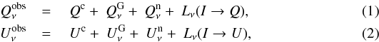 where the term L corresponds to the BPM
leakage map for Galactic emission, offset, and residual dipole. All of them are computed
using the coupling coefficient of each detector to the sky emission spectrum together
with the actual sky scanning strategy. The superscript c represents the CMB polarization,
n represents the noise and
the index G incorporates all
the Galactic emission components in intensity at Planck frequencies. We
restrict our analysis to intermediate Galactic latitudes where the dominant Galactic
emission at HFI frequencies is dust emission. The polarized HFI maps we used are
corrected for the dust, CO, offset and residual dipole, to a first approximation, using
sky measurements of the spectral transmission of each bolometer (Planck Collaboration IX 2014). At LFI frequencies, we correct for BPM
coming from the low frequency Galactic components, i.e., the AME, synchrotron and
free-free emission (Planck Collaboration III
2014), using sky measurements of the spectral transmission of each bolometer.
where the term L corresponds to the BPM
leakage map for Galactic emission, offset, and residual dipole. All of them are computed
using the coupling coefficient of each detector to the sky emission spectrum together
with the actual sky scanning strategy. The superscript c represents the CMB polarization,
n represents the noise and
the index G incorporates all
the Galactic emission components in intensity at Planck frequencies. We
restrict our analysis to intermediate Galactic latitudes where the dominant Galactic
emission at HFI frequencies is dust emission. The polarized HFI maps we used are
corrected for the dust, CO, offset and residual dipole, to a first approximation, using
sky measurements of the spectral transmission of each bolometer (Planck Collaboration IX 2014). At LFI frequencies, we correct for BPM
coming from the low frequency Galactic components, i.e., the AME, synchrotron and
free-free emission (Planck Collaboration III
2014), using sky measurements of the spectral transmission of each bolometer.
To test the results presented in this paper for systematic effects, we use multiple data sets that include the maps made with two independent groups of four PSBs (detector sets “DS1” and “DS2”, see Table 3 in Planck Collaboration VI 2014), the half-ring maps (using the first or second halves of the data from each stable pointing period, “HR1” and “HR2”) and maps made with yearly surveys (“YR1”,“YR2”, etc.). The HR1 and HR2 maps are useful to assess the impact on our data analysis of the noise and systematic effects on scales smaller than 20′. The YR1 map is a combination of first two surveys S1 and S2, and YR2 is a combination of surveys S3 and S4, and so on. The maps made with individual sky surveys are useful to quantify the impact of systematic effects on larger angular scales, particularly from beam ellipticity and far sidelobes (Planck Collaboration III 2014; Planck Collaboration VI 2014). For the intensity and polarization HFI data, we use the two yearly maps YR1 and YR2, whereas for LFI data, we use the four yearly maps grouped into odd (YR1+YR3) and even (YR2+YR4) pairs because they share the same scanning strategy.
The different data sets are independent observations of the same sky that capture noise and systematic effects. They provide means to assess the validity and self-consistency of our analysis of the Planck data. The different map combinations highlight different systematic effects on various timescales and across different dimensions.
-
Half-ring maps share the same scanning strategy and detectors so they have the same leakage from intensity to polarization. The difference between these two maps shows the noise that is not correlated. The removal of glitches induce some noise correlation between the two half-ring maps that affects the data at all multipoles.
-
The differences between two yearly maps is used to check the consistency of the data over the full duration of the Planck mission.
-
Detector set maps have the same combination of scans. The difference between detector set maps show all systematic effects associated with specific detectors.
2.2. WMAP data
We use the WMAP nine year data (Bennett et al. 2013) from the Legacy Archive for Microwave Background Data Analysis (LAMBDA)3 provided in the HEALPix pixelization scheme with a resolution Nside = 512. WMAP observed the sky in five frequency bands, denoted K, Ka, Q, V, and W, centred at the frequencies 23, 33, 41, 61, and 94 GHz, respectively. WMAP has ten differencing assemblies (DAs), one for both K and Ka bands, two for Q band, two for V band, and four for W band. WMAP has frequency-dependent resolution, ranging from 52′ (K band) to 12′ (W band). Multiple DAs at each frequency for Q, V and W bands are combined using simple average to generate a single map per frequency band.
2.3. Ancillary data
We complement the Planck and WMAP data with several ancillary sky maps. We use the 408 MHz map from Haslam et al. (1982), and Hα map from Dickinson et al. (2003, DDD) as tracers of synchrotron and free-free emission, respectively. No dust extinction correction (fd = 0.0) has been applied to the DDD Hα map, which is expressed in units of Rayleigh (R). For our simulations we use the Leiden/Argentine/Bonn (LAB) survey of Galactic Hi column density (Kalberla et al. 2005) as a tracer of dust emission (Planck Collaboration XXIV 2011; Planck Collaboration Int. XVII 2014). Finally, we use the DIRBE 100 μm sky map to determine the dust temperature, like in Planck Collaboration XI (2014).
The 408 MHz, LAB Hi, and DIRBE 100 μm data are downloaded from LAMBDA. We use the DIRBE data corrected for ZLE. We project the DIRBE 100 μm map on a HEALPix grid at Nside = 512 with a Gaussian interpolation kernel that reduces the angular resolution to 50′. Both the 408 MHz and the DDD Hα maps are provided at 1° resolution. The LAB Hi survey and DIRBE 100 μm data have angular resolutions of 36′ and 50′, respectively.
3. Global mask
In the data analysis we use a global mask, shown in Fig. 1, which selects regions of dust emission from the ISM at intermediate Galactic latitudes. We only want to study polarization in regions where thermal dust emission dominates. This means that we need to remove the area around the Galactic plane, where other Galactic contributions are significant, and remove the high latitude regions, where the anisotropies of the cosmic infrared background (CIB) are important with respect to dust emission. The global mask combines thresholds on several sky emission components (in intensity): carbon monoxide (CO) line emission; free-free; synchrotron; the CIB anisotropies; and point sources. We now detail how the global mask is defined.
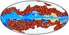 |
Fig. 1 Global mask used in the cross-correlation (CC) analysis (Mollweide projection in Galactic coordinates). It comprises the CIB mask (white region), the CO mask (light-blue), the free-free mask (beige), the Galactic mask (deep-blue), and the mask of point sources (turquoise). We use the red regions of the sky. We refer readers to Sect. 3 for a detailed description of how the global mask is defined. |
In the regions of lowest dust column density at high Galactic latitudes, brightness
fluctuations from the CIB are significant. To define the CIB mask, we apply a threshold on
the ratio between the root mean square (rms) of the total Galactic emission and of the CIB
at 353 GHz:
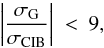 (3)where σG and
σCIB are defined as
(3)where σG and
σCIB are defined as
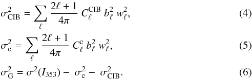 For this threshold, the CIB contribution to the
CC coefficients in Sect. 4.2 is smaller than about 1%
(1 / 92) of that of
the total Galactic emission at 353 GHz. The summation is over the multipole range 15 <ℓ< 300
(corresponding to an effective range of angular scales from 1° to 10°).
For this threshold, the CIB contribution to the
CC coefficients in Sect. 4.2 is smaller than about 1%
(1 / 92) of that of
the total Galactic emission at 353 GHz. The summation is over the multipole range 15 <ℓ< 300
(corresponding to an effective range of angular scales from 1° to 10°).  is the best-fit CIB power spectrum at
353 GHz (Planck Collaboration XXX 2014),
is the best-fit CIB power spectrum at
353 GHz (Planck Collaboration XXX 2014),  is the best-fit CMB power spectrum (Planck Collaboration XV 2014), I353 represents
the Planck353 GHz map, bℓ is the beam function
and wℓ is the HEALPix pixel window function. We measure the
Galactic to CIB emission ratio over patches with 10° radius centred on HEALPix pixels at a resolution Nside = 32.
is the best-fit CMB power spectrum (Planck Collaboration XV 2014), I353 represents
the Planck353 GHz map, bℓ is the beam function
and wℓ is the HEALPix pixel window function. We measure the
Galactic to CIB emission ratio over patches with 10° radius centred on HEALPix pixels at a resolution Nside = 32.
The CO, free-free, and synchrotron emission are more important close to the Galactic plane. The first three CO line transitions J = 1 → 0, J = 2 → 1, and J = 3 → 2 at 115, 230, and 345 GHz, respectively, are significant emission components in the Planck intensity maps (Planck Collaboration XIII 2014). The CO mask is defined by applying a threshold of 0.5 K km s-1 on the “Type 2” CO J = 1 → 0, which is extracted using the Planck data between 70 and 353 GHz (Planck Collaboration XIII 2014). The free-free emission is weak compared to the CO line emission at 100 GHz for most molecular clouds. In massive star-forming regions and for the diffuse Galactic plane emission, free-free emission is significant (Planck Collaboration Int. XIV 2014). We take the WMAP maximum entropy method free-free map (Bennett et al. 2013) at 94 GHz and apply a threshold of 10 μKRJ (in Rayleigh-Jeans temperature units) to define the free-free mask. In addition, we use the Galactic mask (CS-CR75) from the Planck component separation results (Planck Collaboration XII 2014) to exclude the synchrotron emission from the Galactic plane and the Galactic “haze” (Planck Collaboration Int. IX 2013). We also apply the Planck point source mask (Planck Collaboration XV 2014).
Our mask focuses on the part of the sky where dust is the dominant emission component at HFI frequencies. This choice makes the spectral leakage from free-free and CO line emissions to polarization maps negligible. After masking we are left with 39% of the sky at intermediate Galactic latitudes (10° < | b | < 60°). The same global mask is used for both intensity and polarization correlation analysis to compare results over the same sky.
4. Cross-correlation method
We use the CC analysis adopted in many studies (Banday et al. 1996; Gorski et al. 1996; Davies et al. 2006; Page et al. 2007; Ghosh et al. 2012; Planck Collaboration Int. XII 2013) to extract the signal correlated with the 353 GHz template in intensity and polarization. The only underlying assumption is that the spatial structure in the 353 GHz template and in the map under analysis are locally correlated. To reduce this assumption, we apply the CC analysis locally over patches of sky of 10° radius (Sect. 4.4). Our choice for the dust template is presented in Sect. 4.1. The methodology is introduced for intensity in Sect. 4.2 and for polarization in Sect. 4.3. The practical implementation of the method is outlined in Sect. 4.4.
4.1. 353 GHz template
We perform the CC analysis locally in the pixel domain using the Planck353 GHz maps of Stokes parameters as representative internal templates for dust emission in intensity (I with the ZLE subtracted) and polarization (Q and U). Our choice of a Planck map as a dust template addresses some of the issues plaguing alternative choices. First, unlike the Hi map, the 353 GHz map traces the dust in both Hi and H2 gas (Reach et al. 1998; Planck Collaboration XXIV 2011; Planck Collaboration Int. XVII 2014). Second, unlike the full-sky Finkbeiner et al. (1999, hereafter FDS) 94 GHz map, the 353 GHz map does not rely on an extrapolation over a large frequency range, from 100 μm to the Planck bands. The main drawback of the 353 GHz template is that it includes CMB and CIB anisotropies. By introducing the global mask, we work with the sky region where the CIB anisotropies are small compared to dust emission. However, the contribution of the CMB to the CC coefficients, most significant at microwave frequencies, needs to be subtracted.
4.2. Intensity
4.2.1. Correlation with the 353 GHz template
For the intensity data, the CC coefficient ( ) is obtained by minimizing the
 expression given by,
 ![Mathematical equation: \begin{equation} \chisquare_{\rm I}\ = \ \sum_{k\,=\,1}^{N_{\rm pix}} \left [ \nI (k) \ - \ \left [\alphaInu\right]_{353}^{\rm 1T} \ \tI (k) - \ a \right ]^2 , \label{eq:4.1} \end{equation}](/articles/aa/full_html/2015/04/aa24088-14/aa24088-14-eq73.png) (7)where Iν and I353 denote
the data and the 353 GHz
template maps, respectively. This is a linear fit and the solution is computed
analytically. Here the CC coefficient is a number in KCMBKCMB-1, as both Iν and I353 are
expressed in KCMB
units. The constant offset, a, takes into account the local mean present in
the template as well as in the data. The sum is over the unmasked pixels,
k, within
a given sky patch. We are insensitive to the residual dipole present at
Planck frequencies because we perform local correlation over
10° radius patches. The
index “1T” represents the
353 GHz correlated
coefficient at a given frequency ν that we obtained using one template only.
(7)where Iν and I353 denote
the data and the 353 GHz
template maps, respectively. This is a linear fit and the solution is computed
analytically. Here the CC coefficient is a number in KCMBKCMB-1, as both Iν and I353 are
expressed in KCMB
units. The constant offset, a, takes into account the local mean present in
the template as well as in the data. The sum is over the unmasked pixels,
k, within
a given sky patch. We are insensitive to the residual dipole present at
Planck frequencies because we perform local correlation over
10° radius patches. The
index “1T” represents the
353 GHz correlated
coefficient at a given frequency ν that we obtained using one template only.
The CC coefficient at a given frequency includes the contribution from all the emission
components that are correlated with the 353 GHz template (Appendix A).
It can be decomposed into the following terms: ![Mathematical equation: \begin{eqnarray} \left[\alphaInu\right]_{353}^{\rm 1T} &=& \alphaI \left(c^1_{353}\right) + \ \alphaInu \left(d_{353}\right) + \ \alphaInu \left(s_{353}\right) \nonumber \\ && + \ \alphaInu \left(f_{353}\right) + \ \alphaInu \left(a_{353}\right) , \label{eq:4.2} \end{eqnarray}](/articles/aa/full_html/2015/04/aa24088-14/aa24088-14-eq78.png) (8)where
(8)where
 , d353,
s353, f353, and
a353 refer to the CMB, dust,
synchrotron, free-free, and AME signals that are correlated with the 353 GHz template, respectively. The CMB CC
coefficient term is achromatic because Eq. (8) is expressed in KCMB units. We neglect the contributions of the three CO
lines, point sources, and the CIB anisotropies, since these are subdominant within our
global mask (Sect. 3). We also neglect the
cross-correlation of the ZLE with the dust template. The chance correlations between the
emission components we neglect and the dust template contribute to the statistical
uncertainties on the dust SED, but do not bias it. We checked this with Monte Carlo
simulations (Appendix B) and repeated our analysis
on HFI maps with the ZLE subtracted. The correlation terms of the synchrotron and AME
components are negligible at ν ≥ 100 GHz, as synchrotron and AME both have a
steep spectrum that falls off fast at high frequencies. The free-free emission is weak
outside the Galactic plane at high frequencies and does not contribute significantly to
the CC coefficients. The synchrotron, AME and free-free terms only become significant at
ν<
100 GHz inside our global mask.
, d353,
s353, f353, and
a353 refer to the CMB, dust,
synchrotron, free-free, and AME signals that are correlated with the 353 GHz template, respectively. The CMB CC
coefficient term is achromatic because Eq. (8) is expressed in KCMB units. We neglect the contributions of the three CO
lines, point sources, and the CIB anisotropies, since these are subdominant within our
global mask (Sect. 3). We also neglect the
cross-correlation of the ZLE with the dust template. The chance correlations between the
emission components we neglect and the dust template contribute to the statistical
uncertainties on the dust SED, but do not bias it. We checked this with Monte Carlo
simulations (Appendix B) and repeated our analysis
on HFI maps with the ZLE subtracted. The correlation terms of the synchrotron and AME
components are negligible at ν ≥ 100 GHz, as synchrotron and AME both have a
steep spectrum that falls off fast at high frequencies. The free-free emission is weak
outside the Galactic plane at high frequencies and does not contribute significantly to
the CC coefficients. The synchrotron, AME and free-free terms only become significant at
ν<
100 GHz inside our global mask.
4.2.2. Correlation with two and three templates
To remove  and
and
 in Eq. (8), we cross-correlate the Planck and WMAP data with
either two or three templates (including the dust template). We use the 353 GHz and the 408 MHz maps for the fit with two
templates, and add the DDD Hα map for the three-template fit. The
expressions that we minimize for these
two cases are
in Eq. (8), we cross-correlate the Planck and WMAP data with
either two or three templates (including the dust template). We use the 353 GHz and the 408 MHz maps for the fit with two
templates, and add the DDD Hα map for the three-template fit. The
expressions that we minimize for these
two cases are ![Mathematical equation: \begin{eqnarray} \chisquare_{\rm I}&=& \sum_{k=1}^{N_{\rm pix}} \left[ \nI (k) - \left[\alphaInu\right]_{353}^{\rm 2T} \ \tI (k) - \left[\alphaInu\right]_{0.408}^{\rm 2T} \ \hI (k) - a \right]^2,\!\! \\ \chisquare_{\rm I}&=& \ \sum_{k=1}^{N_{\rm pix}} \left[ \nI (k) - \ \left[\alphaInu\right]_{353}^{\rm 3T} \ \tI (k) - \ \left[\alphaInu\right]_{0.408}^{\rm 3T} \ \hI (k) \right. \nonumber\\ && \left. - \ \left[\alphaInu\right]_{\halpha}^{\rm 3T} \ \fI (k) - \ a \right]^2 , \end{eqnarray}](/articles/aa/full_html/2015/04/aa24088-14/aa24088-14-eq88.png) where Iν, I353,
I0.408, and IHα denote the data at
a frequency ν, the Planck353 GHz, Haslam 408 MHz, and DDD
Hα maps,
respectively. For these multiple template fits, the CC coefficients are given by
where Iν, I353,
I0.408, and IHα denote the data at
a frequency ν, the Planck353 GHz, Haslam 408 MHz, and DDD
Hα maps,
respectively. For these multiple template fits, the CC coefficients are given by
![Mathematical equation: \begin{eqnarray} \left[\alphaInu\right]_{353}^{\rm 2T}&=& \ \alphaI \left(c^2_{353}\right) + \ \alphaInu \left(d_{353}\right) + \ \alphaInu (f_{353}) + \ \alphaInu (a_{353}) \label{eq:4.3} \\ \left[\alphaInu\right]_{353}^{\rm 3T}&=& \ \alphaI \left(c^3_{353}\right) + \ \alphaInu \left(d_{353}\right) + \ \alphaInu (a_{353}) . \label{eq:4.4} \end{eqnarray}](/articles/aa/full_html/2015/04/aa24088-14/aa24088-14-eq91.png) The indices “2T” and “3T” are used here to distinguish the CC
coefficients for the fit with two and three templates, respectively. The use of
additional templates removes the corresponding terms from the right hand side of these
equations. Equation (12) is used to
derive the mean dust SED in intensity. Equations (8), (11), and (12) may be combined to derive
and
.
The indices “2T” and “3T” are used here to distinguish the CC
coefficients for the fit with two and three templates, respectively. The use of
additional templates removes the corresponding terms from the right hand side of these
equations. Equation (12) is used to
derive the mean dust SED in intensity. Equations (8), (11), and (12) may be combined to derive
and
.
4.3. Polarization
For the polarization data, we cross-correlate both the Stokes Q and U353 GHz templates with the Q and U maps for all Planck and WMAP frequencies. Ideally in CC analysis, the template is free from noise, but the Planck353 GHz polarization templates do contain noise, which may bias the CC coefficients. To circumvent this problem, we use two independent Q and U maps made with the two detector sets DS1 and DS2 at 353 GHz as templates (Sect. 2.1.2). The maps made with each of the two detector sets have independent noise and dust BPM. Using two polarization detector sets at 353 GHz with independent noise realizations reduces the noise bias in the determination of the 353 GHz CC coefficients. We use the detector set maps rather than the half-ring maps because the removal of glitches induces some noise correlation between the two half-ring maps that affects the data at all multipoles (Planck Collaboration VI 2014; Planck Collaboration X 2014).
The polarization CC coefficient (  ) is derived by minimizing the
  expression given by
 ![Mathematical equation: \begin{eqnarray} \chisquare_{\rm P}&=& \sum_{i=1}^2 \sum_{k=1}^{N_{\rm pix}}\ \left[ \StokesQ_{\nu} (k) - \ \left[\alphaPnu\right]_{353}^{\rm 1T} \ \StokesQ_{353}^i (k)- \ a \right]^2 \nonumber \\ && + \ \left [ \StokesU_{\nu} (k) - \ \left[\alphaPnu\right]_{353}^{\rm 1T} \ \StokesU_{353}^i (k) - \ b \right ]^2 , \label{eq:4.5} \end{eqnarray}](/articles/aa/full_html/2015/04/aa24088-14/aa24088-14-eq96.png) (13)where the index i takes the values 1 and 2,
which correspond to the DS1 and DS2 maps at 353 GHz. The summation k is over the unmasked pixels within a given sky
patch. The constant offsets a and b take into account the local mean present in the
template as well as in the data Stokes Q and U maps, respectively. At 353 GHz, we cross-correlate the DS1 and DS2
maps of Q and
U among
themselves, minimizing
(13)where the index i takes the values 1 and 2,
which correspond to the DS1 and DS2 maps at 353 GHz. The summation k is over the unmasked pixels within a given sky
patch. The constant offsets a and b take into account the local mean present in the
template as well as in the data Stokes Q and U maps, respectively. At 353 GHz, we cross-correlate the DS1 and DS2
maps of Q and
U among
themselves, minimizing ![Mathematical equation: \begin{eqnarray} \chisquare_{\rm P}&=& \sum_{\substack{i=1\\ i \neq j}}^2 \sum_{k=1}^{N_{\rm pix}} \ \left[ \StokesQ_{353}^j (k) - \ \left[\alphaPt\right]_{353}^{\rm 1T} \ \StokesQ_{353}^i (k) - \ a\right]^2 \nonumber \\ && + \ \left [ \StokesU_{353}^j (k) - \ \left[\alphaPt\right]_{353}^{\rm 1T} \ \StokesU_{353}^i (k) - \ b \right ]^2 . \end{eqnarray}](/articles/aa/full_html/2015/04/aa24088-14/aa24088-14-eq99.png) (14)The CC coefficients, , comprise the contributions of CMB, dust,
synchrotron and possibly AME polarization. The free-free polarization is expected to be
negligible theoretically (Rybicki & Lightman
1979) and has been constrained to a few percent observationally (Macellari et al. 2011). The polarization decomposition
is given by
(14)The CC coefficients, , comprise the contributions of CMB, dust,
synchrotron and possibly AME polarization. The free-free polarization is expected to be
negligible theoretically (Rybicki & Lightman
1979) and has been constrained to a few percent observationally (Macellari et al. 2011). The polarization decomposition
is given by ![Mathematical equation: \begin{equation} \left[\alphaPnu\right]^{\rm 1T}_{353} = \ \alphaP \left(c^1_{353}\right) + \ \alphaPnu \left(d_{353}\right) + \ \alphaPnu \left(s_{353}\right) + \ \alphaPnu \left(a_{353}\right) . \label{eq:4.6} \end{equation}](/articles/aa/full_html/2015/04/aa24088-14/aa24088-14-eq100.png) (15)The polarized CMB CC coefficient,
(15)The polarized CMB CC coefficient,
 , is achromatic because Eq. (15) is expressed in KCMB units. Unlike for intensity,
due to the absence of any polarized synchrotron template free from Faraday rotation (Gardner & Whiteoak 1966), we cannot perform a fit
with two templates to remove
, is achromatic because Eq. (15) is expressed in KCMB units. Unlike for intensity,
due to the absence of any polarized synchrotron template free from Faraday rotation (Gardner & Whiteoak 1966), we cannot perform a fit
with two templates to remove  in Eq. (15).
We have performed Monte Carlo simulations at the HFI frequencies in order to estimate the uncertainty on the CC coefficient induced by the noise and other Galactic emission present in the data (see Appendix B).
4.4. Implementation
Here we describe how we implement the CC method. The Planck, WMAP, Hi and DIRBE sky maps are smoothed to a common resolution of 1°, taking into account the effective beam response of each map, and reduced to a HEALPix resolution Nside = 128. For the Planck and WMAP maps, we use the effective beams defined in multipole space that are provided in the Planck Legacy Archive4 (PLA) and LAMBDA website (Planck Collaboration VII 2014; Planck Collaboration IV 2014; Bennett et al. 2013). The Gaussian approximation of the average beam widths for Planck and WMAP maps are quoted in Table 1. For the Hi and DIRBE maps, we also use Gaussian beams with the widths given in Table 1. For the polarization data, we use the “ismoothing” routine of HEALPix that decomposes the Q and U maps into E and Baℓms, applies Gaussian smoothing of 1° in harmonic space (after deconvolving the effective azimuthally symmetric beam response for each map), and transforms the smoothed E and Baℓms back into Q and U maps at Nside = 128 resolution.
We divide the intermediate Galactic latitudes into sky patches with 10° radius centred on HEALPix pixels for Nside = 8. For a
much smaller radius we would have too few independent sky pixels within a given sky patch
to measure the mean dust SED. For a much larger radius we would have too few sky patches
to estimate the statistical uncertainty on the computation of the mean dust SED. Each sky
patch contains roughly 1500 pixels at Nside = 128 resolution. We only consider
400 sky patches (Nbins), which have 500 or more unmasked
pixels. We then cross-correlate the 353 GHz Planck internal template with the WMAP and
Planck maps between 23 and 353 GHz, locally in each sky patch to extract the 353 GHz correlated emission in intensity,
along with its polarization counterpart. The sky patches used are not strictly
independent. Each sky pixel is part of a few sky patches, which is required to sample
properly the spatial variations of the CC coefficients. The mean number of times each
pixel is used in CC coefficients (Nvisit) is estimated with the following
formula:  (16)where
  is the total number of pixels at
1° resolution, 0.39 is the
fraction of the sky used in our analysis and ⟨
Npixels ⟩ = 1000 is the average number of
pixels per sky patch after masking.
is the total number of pixels at
1° resolution, 0.39 is the
fraction of the sky used in our analysis and ⟨
Npixels ⟩ = 1000 is the average number of
pixels per sky patch after masking.
5. Component separation methodology
At the highest frequencies (ν ≥ 100 GHz) within our mask, the two main contributors to the CC coefficient are the CMB and dust emission. In this section, we detail how we separate them and estimate the spectral index of the dust emission (βd) in intensity and polarization.
5.1. Separation of dust emission for intensity
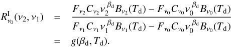
The CC coefficients at ν
≥ 100 GHz can be written as ![Mathematical equation: \begin{equation} \left[\alphaInu\right]_{353}^{\rm 3T} = \ \alphaI \left(c^3_{353}\right) + \ \alphaInu\left(d_{353}\right) , \label{eq:5.1} \end{equation}](/articles/aa/full_html/2015/04/aa24088-14/aa24088-14-eq114.png) (17)where
(17)where  and d353 are the
353 GHz correlated CMB and
dust emission, respectively. The CMB CC coefficient is achromatic in KCMB units, i.e., in temperature
units relative to the CMB blackbody spectrum. To remove the CMB contribution, we work with
the differences of CC coefficients between two given frequencies. To measure the dust
spectral index both in intensity and polarization, we choose to work with colour ratios
defined between two given frequencies ν2 and ν1 as
and d353 are the
353 GHz correlated CMB and
dust emission, respectively. The CMB CC coefficient is achromatic in KCMB units, i.e., in temperature
units relative to the CMB blackbody spectrum. To remove the CMB contribution, we work with
the differences of CC coefficients between two given frequencies. To measure the dust
spectral index both in intensity and polarization, we choose to work with colour ratios
defined between two given frequencies ν2 and ν1 as
![Mathematical equation: \begin{eqnarray} R_{\nu_0}^{\rm I}(\nu_2,\nu_1)&=& \dfrac{\left[\alpha_{\nu_2}^{\rm I}\right]_{353}^{\rm 3T} -\left[\alpha_{\nu_0}^{\rm I}\right]_{353}^{\rm 3T} }{\left[\alpha_{\nu_1}^{\rm I}\right]_{353}^{\rm 3T} -\left[\alpha_{\nu_0}^{\rm I}\right]_{353}^{\rm 3T} } = \dfrac{\alpha_{\nu_2}^{\rm I}\left(d_{353}\right)-\alpha_{\nu_0}^{\rm I}\left(d_{353}\right)}{\alpha_{\nu_1}^{\rm I}\left(d_{353}\right)-\alpha_{\nu_0}^{\rm I}\left(d_{353}\right)} , \label{eq:5.2} \end{eqnarray}](/articles/aa/full_html/2015/04/aa24088-14/aa24088-14-eq118.png) (18)where ν0 represents
the reference CMB frequency which is chosen to be 100 GHz in the present analysis. To
convert the measured colour ratio into βd we follow earlier studies (Planck Collaboration Int. XVII 2014; Planck Collaboration XI 2014) by approximating the SED
of the dust emission with a modified blackbody (MBB) spectrum (Planck Collaboration XXV 2011; Planck
Collaboration XXIV 2011; Planck Collaboration XI
2014) given by
(18)where ν0 represents
the reference CMB frequency which is chosen to be 100 GHz in the present analysis. To
convert the measured colour ratio into βd we follow earlier studies (Planck Collaboration Int. XVII 2014; Planck Collaboration XI 2014) by approximating the SED
of the dust emission with a modified blackbody (MBB) spectrum (Planck Collaboration XXV 2011; Planck
Collaboration XXIV 2011; Planck Collaboration XI
2014) given by  (19)where Td is the colour
temperature and βd is the spectral index of the dust
emission. The factor Fν takes into account
the conversion from MJy sr-1 (with the photometric convention νIν =
constant) to KCMB
units, while Cν is the colour
correction that depends on the value of βd and Td. The colour
correction is computed knowing the bandpass filters at the HFI frequencies (Planck Collaboration IX 2014) and the spectrum of the
dust emission. Using Eq. (19), the colour
ratio can be written as a function of βd and Td:
(19)where Td is the colour
temperature and βd is the spectral index of the dust
emission. The factor Fν takes into account
the conversion from MJy sr-1 (with the photometric convention νIν =
constant) to KCMB
units, while Cν is the colour
correction that depends on the value of βd and Td. The colour
correction is computed knowing the bandpass filters at the HFI frequencies (Planck Collaboration IX 2014) and the spectrum of the
dust emission. Using Eq. (19), the colour
ratio can be written as a function of βd and Td:
 (20)In Sect. 6.1, we use the three Planck maps, at 100, 217, and 353 GHz, to compute
 and measure the dust spectral index
(
and measure the dust spectral index
( ) at microwave frequencies (or mm
wavelengths), for each sky patch. In the next section, we explain how we determine
Td.
) at microwave frequencies (or mm
wavelengths), for each sky patch. In the next section, we explain how we determine
Td.
5.2. Measuring colour temperatures in intensity
The dust temperatures inferred from an MBB fit of the Planck at
ν ≥ 353 GHz
and the IRAS 100 μm sky maps at 5′ resolution (Planck Collaboration XI 2014) cannot be used to compute mean
temperatures within each sky patch because the fits are nonlinear. The two frequencies,
Planck 857 GHz and DIRBE 100 μm (3000 GHz), which are close to the dust emission
peak, are well suited to measure Td for each sky patch. We use the
Planck353 GHz map as a template to compute the colour ratio RI(3000,857)
over each sky patch, as described in Eq. (18). The superscript I on the colour ratio and βd denote intensity. As the CMB signal
is negligible at these frequencies, we work directly with the ratio RI(3000,857),
without subtracting the 100 GHz CC measure. We assume a mean dust spectral index at submm
frequencies,  , of 1.50. The choice of
value is based on the MBB fit to the dust
emissivities at 100 μm and the Planck 353, 545 and 857
GHz frequencies, for each sky patch. Due to the – Td
anti-correlation, the variations of the values just increases the scatter of the
Td values by about 20% as compared to
Td values derived using fixed
. However, the Td values from
the MBB fits are closely correlated with Td values determined using the ratio
RI(3000,857) and a fixed spectral index.
We use the colour ratio RI(3000,857) and mean
, of 1.50. The choice of
value is based on the MBB fit to the dust
emissivities at 100 μm and the Planck 353, 545 and 857
GHz frequencies, for each sky patch. Due to the – Td
anti-correlation, the variations of the values just increases the scatter of the
Td values by about 20% as compared to
Td values derived using fixed
. However, the Td values from
the MBB fits are closely correlated with Td values determined using the ratio
RI(3000,857) and a fixed spectral index.
We use the colour ratio RI(3000,857) and mean
 to estimate Td values for
each sky patch by inverting the relation given in Eq. (20).
to estimate Td values for
each sky patch by inverting the relation given in Eq. (20).
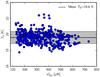 |
Fig. 2 Dust colour temperatures, Td, computed from RI(3000,857), are plotted versus the
local dispersion of the 353 GHz intensity template,
|
In Fig. 2, we plot the derived Td versus the
local brightness dispersion of the Planck353 GHz template in intensity
( ). We point out that
is not an uncertainty in the
353 GHz intensity template.
The mean value of Td over our mask at intermediate
Galactic latitudes is 19.6 K.
The 1σ
dispersion of Td over the 400 sky patches is
0.8 K. This value is
slightly smaller that the mean value at high Galactic latitudes, 20.4 ± 1.1 K for
). We point out that
is not an uncertainty in the
353 GHz intensity template.
The mean value of Td over our mask at intermediate
Galactic latitudes is 19.6 K.
The 1σ
dispersion of Td over the 400 sky patches is
0.8 K. This value is
slightly smaller that the mean value at high Galactic latitudes, 20.4 ± 1.1 K for
 5, we
obtained repeating the dust-Hi correlation analysis of Planck Collaboration Int. XVII (2014) on the same full-mission
Planck data.
5, we
obtained repeating the dust-Hi correlation analysis of Planck Collaboration Int. XVII (2014) on the same full-mission
Planck data.
The choice of used in this paper is different from the
one derived from the analysis of high Galactic latitude data (Planck Collaboration Int. XVII 2014) and the analysis of the whole sky
(Planck Collaboration XI 2014) using public
release Planck 2013 data. This difference results from a change in the
photometric calibration by 1.9%, −
2.2%, − 3.5%,
at 353, 545 and 857 GHz,
between the DX11d and the Planck 2013 data. The new calibration factors
make the mean slightly smaller and Td slightly
higher. To estimate uncertainties on , we run a set of Monte-Carlo simulations
that take into account the absolute and relative calibration uncertainties present in the
DIRBE and the Planck full-mission HFI data at ν ≥ 353 GHz. We assume that
the MBB spectrum is a good fit to the data and apply 1σ photometric
uncertainties of 1%, 7%, 7%, and 13% at 353, 545, 857, and 3000 GHz respectively. To get
multiple SED realizations, we vary the MBB spectrum within the photometric uncertainty at
each frequency used for the fit, independently of others. Then we perform the MBB SED fit
and find that the 1σ dispersion on the mean value of
is 0.16 (syst.). The new value
of is well within the range of values and
systematic uncertainties quoted in Table 3 of Planck
Collaboration XI (2014, using 2013
Planck data) for the same region of the sky.
5.3. Separation of CMB emission in intensity
The CC coefficient, derived in Eq. (8),
contains the CMB contribution that is achromatic in KCMB units. We determine this CMB
contribution assuming that the dust emission is well approximated by a MBB spectrum from
100 to 353 GHz. For each sky
patch, we use the values of and Td from Sects.
6.1 and 5.2.
We solve for two parameters, the CMB contribution,  , and the dust amplitude,
 , by minimizing
![Mathematical equation: \begin{equation} \chi_{\rm s}^2 = \sum_{\nu}\ \left ( \frac{\left[\alphaInu\right]_{353}^{\rm 3T} - \alpha^{\rm I} \left(c^3_{353}\right) - F_{\nu}\ C_{\nu} \ A_{\rm d}^{\rm \StokesI} \ \nu^{\ \beta_{\rm d,mm}^{\rm I}} \ B_{\nu} \left(\Td\right) }{\sigma_{\alphaInu}} \right )^2 , \end{equation}](/articles/aa/full_html/2015/04/aa24088-14/aa24088-14-eq144.png) (21)where
(21)where  is the uncertainty on the CC coefficient,
determined using the Monte Carlo simulations (Appendix B). The joint spectral fit of , , Td, and
leads to a degeneracy between the fitted
parameters. To avoid this problem, we fix the values of
and Td for each sky
patch based on the colour ratios, independent of the value of
. The CMB contributions are subtracted from
the CC coefficients at all frequencies, including the LFI and WMAP data not used in the
fit. After CMB subtraction, the CC coefficient (
is the uncertainty on the CC coefficient,
determined using the Monte Carlo simulations (Appendix B). The joint spectral fit of , , Td, and
leads to a degeneracy between the fitted
parameters. To avoid this problem, we fix the values of
and Td for each sky
patch based on the colour ratios, independent of the value of
. The CMB contributions are subtracted from
the CC coefficients at all frequencies, including the LFI and WMAP data not used in the
fit. After CMB subtraction, the CC coefficient ( ) for the 353 GHz template is
 ![Mathematical equation: \begin{equation} \left[\tildealphaInu\right]_{353}^{\rm 3T} = \left[\alphaInu\right]_{353}^{\rm 3T} - \alpha^{\rm I} \left(c^3_{353}\right) = \ \alphaInu \left(d_{353}\right) .\label{eq:6.1} \end{equation}](/articles/aa/full_html/2015/04/aa24088-14/aa24088-14-eq147.png) (22)We perform the same exercise on the one- and
two-template fits to derive the CMB subtracted CC coefficients.
(22)We perform the same exercise on the one- and
two-template fits to derive the CMB subtracted CC coefficients.
5.4. Separation of dust emission for polarization
As for our analysis of the intensity data, we write the 353 GHz correlated polarized CC
coefficients at ν ≥
100 GHz as ![Mathematical equation: \begin{equation} \left[\alphaPnu\right]_{353}^{\rm 1T} = \ \alphaP \left(c^1_{353}\right) + \ \alphaPnu\left(d_{353}\right) , \label{eq:5.4.1} \end{equation}](/articles/aa/full_html/2015/04/aa24088-14/aa24088-14-eq148.png) (23)where and d353 are the CMB
and dust polarized emission correlated with the 353 polarization templates. The contributions from synchrotron and AME
to the polarized CC coefficients are assumed to be negligible at HFI frequencies. Like for
intensity in Eq. (20), we compute
(23)where and d353 are the CMB
and dust polarized emission correlated with the 353 polarization templates. The contributions from synchrotron and AME
to the polarized CC coefficients are assumed to be negligible at HFI frequencies. Like for
intensity in Eq. (20), we compute
 combining the three polarized CC
coefficients at 100, 217 and 353
GHz. We assume that the temperature of the dust grains contributing to
the polarization is the same as that determined for the dust emission in intensity (Sect.
5.2), and derive
combining the three polarized CC
coefficients at 100, 217 and 353
GHz. We assume that the temperature of the dust grains contributing to
the polarization is the same as that determined for the dust emission in intensity (Sect.
5.2), and derive
 at microwave frequencies.
To separate the contribution of dust and the CMB to the polarized CC coefficients, we follow the method described in Sect. 5.3, and rely on the Monte Carlo simulations described in Appendix B to estimate uncertainties. The CMB contribution is subtracted at all frequencies, including the LFI and WMAP data.
6. Dust spectral index for intensity
Here we estimate the dust spectral index at microwave frequencies (ν ≤ 353 GHz) and mm
wavelengths. We present the results of the data analysis and estimate the uncertainties,
including possible systematic effects.
6.1. Measuring 
 |
Fig. 3 Top: colour ratio |
We use the three full mission Planck maps, at 100, 217, and 353 GHz, to derive a mean
using the three-template fit, assuming an
MBB spectrum for the dust emission (Sect. 5.1). The
217 and 353 GHz maps have the
highest signal-to-noise ratio for dust emission at microwave frequencies, whereas the
100 GHz map is used as a
reference frequency to subtract the CMB contribution at the CC level. We estimate
for each sky patch using the relation
given by Eq. (18). The values of
are plotted in top panel of Fig. 3 as a function of
, which allows us to identify the
statistical noise and systematic effects due to uncertainties on the CC coefficients. Our
Monte Carlo simulations (Appendix B) show that the
uncertainties on scale approximately as the inverse
square-root of , and that the scatter in the measured
for sky patches with low
is due to data noise.
For each sky patch, we derive from
by inverting Eq. (20) for the values of Td derived in
Sect. 5.2. The histogram of
for all sky patches is presented in the
bottom panel of Fig. 3. The mean value of
from the 400 sky patches is 1.514
(round-off to 1.51) with 1σ dispersion of 0.065 (round-off to 0.07). The
statistical uncertainty on the mean is 0.01, which is computed from the
1σ
deviation divided by the square root of the number of independent sky patches
(400/Nvisit) used. This estimate of the
statistical error bar on takes into account the uncertainties
associated with the chance correlation between the dust template and emission components
(CO lines, point sources, the CIB anisotropies and the ZLE) not fitted with templates. It
also includes uncertainties on the subtraction of the CMB contribution.
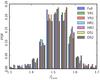 |
Fig. 4 Same plot as in the bottom panel of Fig. 3,
including our results for the subsets of the Planck data listed in
Table 2. The bin per bin measurements of
|
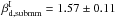
6.2. Uncertainties on
We use the full mission Planck intensity maps as a reference data for
the mean dust spectral index value. To assess the systematic uncertainties on the mean
spectral index, we repeat our CC analysis on maps made with subsets of the
Planck data (Sect. 2.1.2), keeping
the same ZLE-subtracted Planck353 GHz map as a template. For each set of maps, we compute the mean
from
values. Table 2 lists the values derived from the three-template fit
applied to each data sub-set. The six measurements of
from various data splits are within the
1σ
statistical uncertainties on the mean intensity dust spectral index. We find a mean dust
spectral index 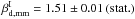 . This spectral index is very close to the
mean index of 1.50 at sub-mm wavelengths we derived from MBB fits to the
Planck data at ν ≥ 353 GHz in Sect. 5.2.
. This spectral index is very close to the
mean index of 1.50 at sub-mm wavelengths we derived from MBB fits to the
Planck data at ν ≥ 353 GHz in Sect. 5.2.
6.3. Dependence of on the choice of

In Fig. 5 we plot
as a function of
and Td. The central
black line corresponds to the median value of obtained using the CC analysis. Figure
5 shows that varying Td by
±2 K, a ±2.5σ deviation from the mean
value, changes by ±0.05. To estimate
, we use Td, which in
turn depends on . We repeat our analysis with two different
starting values of , which are within 1σ systematics uncertainties
derived in Sect. 5.2. For the values of
 and 1.66, we find
 and 1.53, respectively. This is due to the
fact that in Rayleigh-Jeans limit, the effect of Td is low, and
the shape of the spectrum is dominated by . Our determination of mean
is robust and independent of the initial
choice of used for the analysis.
and 1.53, respectively. This is due to the
fact that in Rayleigh-Jeans limit, the effect of Td is low, and
the shape of the spectrum is dominated by . Our determination of mean
is robust and independent of the initial
choice of used for the analysis.
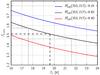 |
Fig. 5 Variation of |

6.4. Alternative approach of measuring
To derive the dust spectral index from , we assume an MBB spectrum for the dust
emission between 100 and 353 GHz (Sect. 5.1). To validate
this assumption, we repeat our CC analysis with Planck maps corrected for
CMB anisotropies using the CMB map from the spectral matching independent component
analysis (SMICA, Planck Collaboration XII 2014). We infer
(SMICA) directly from the ratio between the
353 and 217 GHz CC
coefficients without subtracting the 100 GHz CC coefficient, i.e., ![Mathematical equation: \begin{equation} R^{\rm I}_{\smica} (353,217) = \dfrac{\left[\alpha'_{353}\right]_{(353-\smica)}^{\rm 1T} }{\left[\alpha'_{217}\right]_{(353-\smica)}^{\rm 1T} } \label{eq:smica} , \end{equation}](/articles/aa/full_html/2015/04/aa24088-14/aa24088-14-eq163.png) (24)where α′ refers to the CC
coefficients computed with maps corrected for CMB anisotropies using the SMICA map. The histogram of the difference
between the two sets of spectral indices and
(SMICA) is presented in Fig. 6. The mean difference between the two estimates is zero.
(24)where α′ refers to the CC
coefficients computed with maps corrected for CMB anisotropies using the SMICA map. The histogram of the difference
between the two sets of spectral indices and
(SMICA) is presented in Fig. 6. The mean difference between the two estimates is zero.
 |
Fig. 6 Histogram of the difference between the spectral indices
|
6.5. Comparison with other studies
Our determination of the spectral index of the dust emission in intensity at
intermediate Galactic latitudes may be compared with the results from similar analyses of
the Planck data. In Planck Collaboration
Int. XVII (2014), the CC analysis has been applied to the Planck
data at high Galactic latitudes (b< −30°) using an Hi map as a dust template free from CIB and CMB
anisotropies. This is a suitable template to derive the spectral dependence of dust
emission at high Galactic latitudes. The same methodology of colour ratios has been used
in that work. The mean dust spectral index,  , from Planck Collaboration Int. XVII (2014) agrees with the mean value we find in this
paper. In an analysis of the diffuse emission in the Galactic plane, the spectral index of
dust at millimetre wavelengths is found to increase from
, from Planck Collaboration Int. XVII (2014) agrees with the mean value we find in this
paper. In an analysis of the diffuse emission in the Galactic plane, the spectral index of
dust at millimetre wavelengths is found to increase from
 , for lines of sight where the medium is
mostly atomic, to
, for lines of sight where the medium is
mostly atomic, to  , where the medium is predominantly
molecular (Planck Collaboration Int. XIV 2014). The
three studies indicate that the spectral index is remarkably similar over the diffuse ISM
observed at high and intermediate Galactic latitudes, and in the Galactic plane.
, where the medium is predominantly
molecular (Planck Collaboration Int. XIV 2014). The
three studies indicate that the spectral index is remarkably similar over the diffuse ISM
observed at high and intermediate Galactic latitudes, and in the Galactic plane.
7. Spectral energy distribution of dust intensity
In this section, we derive the mean SED of dust emission for intensity with its uncertainties from our CC analysis. The detailed spectral modelling of the dust SED is discussed in Sect. 7.2.
7.1. Mean dust SED
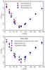 |
Fig. 7 Top: the three SEDs in KRJ units, normalized to 1 at 353 GHz, obtained by averaging, CMB corrected, CC coefficients from the fits with one (cyan circles), two (blue circles) and three templates (red circles). The uncertainties at each frequency are estimated using the subsets of Planck and WMAP data. Bottom: our SED from the three-template fit (red circles) is compared with the dust SED in Planck Collaboration Int. XII (2013) for the Gould Belt system (squares) and that at high latitude sky (inverted triangles) obtained applying the dust-Hi correlation analysis in Planck Collaboration Int. XVII (2014) to the full Planck mission data. |
We use the full mission Planck maps for the spectral modelling of the dust SED in intensity. The mean SED is obtained by averaging the CC coefficients after CMB subtraction (see Sect. 5.3) over all sky patches. The mean SED is expressed in KRJ units, normalized to 1 at 353 GHz. The three SEDs obtained from the fits with one, two, and three templates are shown in Fig. 7. The SED values obtained with the three templates fit are listed in Table 3. The three SEDs are identical at the highest frequencies. They differ at ν< 100 GHz due to the non-zero correlation between the 353 GHz dust template with synchrotron and free-free emission. At 23 GHz, after CMB correction the CC coefficient from the fit with three templates is lower by 9 and 35% from those derived from the fits with two and one template, respectively. The 9% difference accounts for the free-free emission correlated with dust and the 35% difference for the combination of both synchrotron and free-free emission correlated with dust. At these low frequencies, the fit with three templates provides the best separation of the dust from the synchrotron and free-free emission. It is this SED that we call the dust SED hereafter.
Our dust SED is similar to that measured for the Gould Belt system (Planck Collaboration Int. XII 2013) and at high Galactic latitudes (Planck Collaboration Int. XVII 2014). It shows the thermal dust emission at ν ≥ 70 GHz and is dominated by AME at lower frequencies. At WMAP frequencies, our dust SED is similar to that obtained using the FDS 94 GHz map as a dust template in Davies et al. (2006) and Ghosh et al. (2012). The mean dust SED derived using the three-template fit depends on the correction of the DDD Hα map for dust scattering and extinction (Dickinson et al. 2003; Witt et al. 2010; Brandt & Draine 2012; Bennett et al. 2013). In Appendix C, we study the impact of both assumptions on the mean dust SED, which are within a few percent at frequencies below 70 GHz and have no impact on frequencies above 100 GHz.
The total uncertainty on the dust SED includes the inter-calibration uncertainties on the
data, the statistical uncertainties estimated from the variations of the CC coefficients
across the sky patches, and the uncertainties due to the CMB subtraction, as discussed for
in Sect. 6.1. The inter-calibration uncertainties (cν) for
Planck and WMAP data are given in Table 3. The statistical uncertainties are computed from the 1σ dispersion of the CC
coefficients over the 400 sky patches divided by the square root of the number of
independent sky patches (400/Nvisit). All three types of uncertainty,
listed in Table 3, are added together in quadrature
to compute the total uncertainty on the mean dust SED. They are shown in Fig. 7, but most do not appear because they are smaller than
the size of the symbols.
Mean microwave SEDs obtained from the fit with one, two, and three templates using the CC analysis.
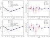 |
Fig. 8 Mean dust SED in KRJ units, normalized to 1 at 353 GHz, with different spectral fits and the respective residuals. The two parametric model fits are DI+AI (top left), and DI+AII (bottom left), as presented in Sect. 7.2. Right: residuals after removing the best fit model listed in Table 4, from the mean dust SED. The two spectral models provide good fit to the data, with residuals compatible with zero. |
7.2. Parametric modelling for intensity dust SED
A spectral fit of the dust SED is required to separate the thermal dust emission from the AME. We continue to use an MBB spectrum for the thermal dust emission, and consider two models with different spectra for the AME.
-
Model DI+AI: in this first approach, we use the analytical model of the AME (AI) introduced by Bonaldi et al. (2007), which is a parabola in the log Iν – log ν plane, parameterized by the peak frequency (νp) and the slope − m60 at 60 GHz. The AME model (Ma) normalized at 23 GHz (in KRJ units) is given by:
![Mathematical equation: \begin{eqnarray} && \log~M_{\rm a} = - \left(\frac{m_{60}\log~\nu_{\rm p}}{\log(\nu_{\rm p}/60\,{\rm GHz})} + 2 \right)\log\left(\frac{\nu}{23\,{\rm GHz}}\right) \nonumber \\ && + \frac{m_{60}}{2\log(\nu_{\rm p}/60\,{\rm GHz})} \left [ \left (\log(\nu/1\,{\rm GHz})\right)^2 - (\log~23)^2 \right ] . \end{eqnarray}](/articles/aa/full_html/2015/04/aa24088-14/aa24088-14-eq196.png) (25)This model is a good fit to spectra of
dipole emission from small spinning dust particles computed with the SPDUST code (Ali-Haïmoud et al. 2009; Silsbee
et al. 2011). The second component is the MBB spectrum of the thermal dust
emission (DI) with free parameter . The total model is written in
KRJ units
normalized to 1 at the frequency νref = 353 GHz:
(25)This model is a good fit to spectra of
dipole emission from small spinning dust particles computed with the SPDUST code (Ali-Haïmoud et al. 2009; Silsbee
et al. 2011). The second component is the MBB spectrum of the thermal dust
emission (DI) with free parameter . The total model is written in
KRJ units
normalized to 1 at the frequency νref = 353 GHz: ![Mathematical equation: \begin{equation} \left\langle\left[\tildealphaInu\right]_{353}^{\rm 3T}\right\rangle = \ A_{\rm a}^{\rm I}\ M_{\rm a} +\ \left(\frac{\nu}{\nuref}\right)^{\beta_{\rm d,mm}^{\rm I} - 2} \frac{B_{\nu} (\Td)}{B_{\nuref} (\Td)} \label{eq:7.2} , \end{equation}](/articles/aa/full_html/2015/04/aa24088-14/aa24088-14-eq198.png) (26)where
(26)where
 is the amplitude of AME and
is the spectral index of thermal
dust emission at microwave frequencies. We fix Td =
19.6 K from Sect. 5.2. The
four free parameters of the model are , m60,
νp and
.
is the amplitude of AME and
is the spectral index of thermal
dust emission at microwave frequencies. We fix Td =
19.6 K from Sect. 5.2. The
four free parameters of the model are , m60,
νp and
. -
Model DI+AII: in this second approach, the AME component (AII) is a linear combination of two spinning dust components arising from the typical cold neutral medium (CNM) and warm neutral medium (WNM). In our analysis, we use the predicted SPDUST (v2) spectra (Ali-Haïmoud et al. 2009; Silsbee et al. 2011) of the CNM and WNM spinning dust components. Following the work of Hoang et al. (2011) and Ghosh et al. (2012), we shift both the WNM and CNM spectra in frequency space to fit the observed dust SED. The same DI model of the thermal dust emission is considered for this model. In this case, the spectral model is given in KRJ units, normalized to 1 at the frequency νref, by:
![Mathematical equation: \begin{eqnarray} \left\langle\left[\tildealphaInu\right]_{353}^{\rm 3T}\right\rangle &=& \ A_{\rm WNM}^{\rm I} \ D_{\rm WNM} \left(\nu - \Delta \nu_{\rm WNM}\right) \nonumber \\[2mm] && + \ A_{\rm CNM}^{\rm I} \ D_{\rm CNM} \left(\nu - \Delta \nu_{\rm CNM}\right) \nonumber \\[2mm] \label{eq:7.3}&& + \ \left(\frac{\nu}{\nuref}\right)^{\beta_{\rm d,mm}^{\rm I} - 2} \frac{B_{\nu} (\Td)}{B_{\nuref} (\Td)} , \end{eqnarray}](/articles/aa/full_html/2015/04/aa24088-14/aa24088-14-eq202.png) (27)where
(27)where
 is the amplitude of WNM spectrum
normalized at 23 GHz,
is the amplitude of WNM spectrum
normalized at 23 GHz,  is the amplitude of CNM spectrum
normalized at 41 GHz, DWNM is the SPDUST WNM spectrum, DCNM is
the SPDUST CNM spectrum,
ΔνWNM is the shift in the WNM
spectrum, ΔνCNM is the shift in the CNM
spectrum, νref = 353 GHz is the reference
frequency, is the spectral index of the thermal
dust emission. We fix
is the amplitude of CNM spectrum
normalized at 41 GHz, DWNM is the SPDUST WNM spectrum, DCNM is
the SPDUST CNM spectrum,
ΔνWNM is the shift in the WNM
spectrum, ΔνCNM is the shift in the CNM
spectrum, νref = 353 GHz is the reference
frequency, is the spectral index of the thermal
dust emission. We fix  from Sect. 6.2 and Td = 19.6 K from Sect. 5.2. The four free parameters of the model are the
WNM amplitude, the WNM frequency shift, the CNM amplitude and the CNM frequency
shift.
from Sect. 6.2 and Td = 19.6 K from Sect. 5.2. The four free parameters of the model are the
WNM amplitude, the WNM frequency shift, the CNM amplitude and the CNM frequency
shift.
The fits of the dust SED with models DI+AI and DI+AII are shown in Fig. 8. The best fit model parameters are listed in Table 4.
Results of the spectral fits to the mean dust SED in intensity using Planck and WMAP maps.
8. Dust spectral index for polarization
We now move to the analysis of the polarization data. Like in Sect. 6, we estimate the polarized dust spectral index
() at microwave frequencies (ν ≤ 353 GHz). We present the
results of our data analysis and tests of its robustness against systematic uncertainties.
8.1. Measuring 
Here we use the full mission Planck polarization maps, keeping the
polarized detector set maps (DS1 and DS2) at 353 GHz as fixed templates, to derive a mean
using the one-template fit. Using the
polarization CC coefficients, ![Mathematical equation: \hbox{$[\alphaPnu]_{353}^{\rm 1T}$}](/articles/aa/full_html/2015/04/aa24088-14/aa24088-14-eq221.png) , we compute
for each sky patch using Eq. (18). Figure 9 shows the values of versus the local dispersion of the
polarized map at 353 GHz
(
, we compute
for each sky patch using Eq. (18). Figure 9 shows the values of versus the local dispersion of the
polarized map at 353 GHz
( ) for all the sky patches. To compute
, we use a 1° smoothed map of P353 derived in
Planck Collaboration Int. XIX (2015). We derive
for each sky patch from
, taking into account the local estimate of
Td derived from RI(3000,857)
(Sect. 5.2). We assume that the temperature of the
dust grains contributing to the polarization is the same as that determined for the dust
emission in intensity. This is not necessarily true if the polarization is associated with
specific dust grains, e.g., the silicates versus carbon dust (Martin 2007; Draine & Fraisse
2009). This should be kept in mind in thinking of physical interpretations. Here
we use the spectral indices and
as a mathematical way to quantify the
difference between the dust SED for intensity and polarization.
) for all the sky patches. To compute
, we use a 1° smoothed map of P353 derived in
Planck Collaboration Int. XIX (2015). We derive
for each sky patch from
, taking into account the local estimate of
Td derived from RI(3000,857)
(Sect. 5.2). We assume that the temperature of the
dust grains contributing to the polarization is the same as that determined for the dust
emission in intensity. This is not necessarily true if the polarization is associated with
specific dust grains, e.g., the silicates versus carbon dust (Martin 2007; Draine & Fraisse
2009). This should be kept in mind in thinking of physical interpretations. Here
we use the spectral indices and
as a mathematical way to quantify the
difference between the dust SED for intensity and polarization.
The scatter on the values increases for
 K due to data noise. The histogram of
from the 400 sky patches is presented in
Fig. 9. The distribution of
has a mean value of 1.592 (round-off to
1.59), with a 1σ dispersion of 0.174 (round-off to 0.17). This
dispersion is the same if we use the mean dust temperature of 19.6 K for all sky patches. The statistical
uncertainty on the mean is computed from the 1σ dispersion divided by
the square root of the number of independent sky patches (400 /Nvisit)
used, which is 0.02.
K due to data noise. The histogram of
from the 400 sky patches is presented in
Fig. 9. The distribution of
has a mean value of 1.592 (round-off to
1.59), with a 1σ dispersion of 0.174 (round-off to 0.17). This
dispersion is the same if we use the mean dust temperature of 19.6 K for all sky patches. The statistical
uncertainty on the mean is computed from the 1σ dispersion divided by
the square root of the number of independent sky patches (400 /Nvisit)
used, which is 0.02.
The mean value of the dust spectral index for polarization is different from that for intensity, 1.51 ± 0.01 (Sect. 6) over the same sky area. In the next section, we check whether the difference of spectral indices in intensity and polarization is a robust result against systematics present in the polarization data.
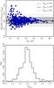 |
Fig. 9 Top: colour ratio |
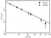 |
Fig. 10 Spectral energy distribution of the dust-correlated synchrotron emission in
intensity. The SED is the ratio between the synchrotron emission at frequency
ν and
the dust emission at 353 GHz emission in units of KRJ. The mean spectral
index for the intensity is |
Polarized dust spectral indices derived using multiple subsets and templates of the Planck data.
8.2. Uncertainties in
For the mean polarized dust spectral index, we use the results from full mission
Planck polarization maps with the two detector set maps as fixed
templates (Sect. 8.1). To estimate the systematic
uncertainty for the mean , we apply the CC analysis on multiple
subsets of the Planck data, including the combination of yearly maps (YR1
and YR2), the full mission half-ring maps (HR1 and HR2), the combination of odd surveys
(S1+S3) and even surveys (S2+S4), and the detector set maps (DS1 and DS2; see Sect. 2.1.2 for more details). We use these subsets of the data
as maps and templates at 353 GHz. Table 5 lists the
derived mean , for all the sky patches from each
combination of the data subsets. The dispersion of the
values in Table 5, 0.02, is consistent with the 1σ dispersion on the mean
polarization spectra index from statistical uncertainties estimated in Sect. 8.1, making it difficult to separate the contributions
from the statistical noise and the data systematics. Therefore, we use the 1σ dispersion from the
subsets of the Planck data, as listed in Table 5, as a combine statistical and systematic uncertainties on the mean
value of . Thus, we find
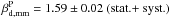 . The small difference, 0.08, between
and
has a 3.6σ significance, taking
into account the total uncertainty on both and
.
. The small difference, 0.08, between
and
has a 3.6σ significance, taking
into account the total uncertainty on both and
.
9. Spectral energy distribution of dust polarization
We now derive the mean SED for the dust polarization and extend to polarization the parametric modelling already made on the dust SED in intensity (Sect. 7.2).
Mean microwave SED for polarization computed using the CC analysis.
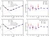 |
Fig. 11 Mean polarized SED in KRJ units, normalized to 1 at 353 GHz correlated with the Stokes
Q and
U353 GHz maps. The polarized spectral model with and without the
constraint on |
9.1. Mean polarized SED
We use the full mission Planck maps for the spectral modelling of the dust SED in polarization. Like in Sect. 7.1 for dust emission in intensity, the mean SED for polarization is obtained by averaging the polarization CC coefficients after CMB subtraction (see Sect. 5.3) over all sky patches and is expressed in KRJ units. The polarization SED is derived from the one-template fit, keeping the templates fixed to the polarized detector set maps (DS1 and DS2) at 353 GHz (see Sect. 4.3 for more details). We compute the mean polarization SED and its uncertainties in a similar manner to that discussed in Sect. 7. The mean polarized SED and associated uncertainties are listed in Table 6, and is shown in Fig. 11.
The polarization SED first decreases with decreasing frequency, then turns up below 60 GHz. This is the first time that such a behavior has been observed for polarized emission correlated with dust polarization, though it has been seen before for the total sky polarization (Bennett et al. 2013).
9.2. Low frequency rise of the polarization SED
In this section, we show that a synchrotron component correlated with dust is the most likely interpretation for the low frequency rise of the polarization SED.
9.2.1. Synchrotron polarization correlated with dust
The polarized dust and synchrotron emissions may be written as
![Mathematical equation: \begin{eqnarray} &&\left[\StokesQ^{\rm s}_{\nu},\StokesU^{\rm s}_{\nu}\right]= \ \polfrac_{\rm s} \ \StokesI^{\rm s}_{\nu} \ \left[\cos 2\polang_{\rm s},\sin 2\polang_{\rm s}\right] , \\ &&\left[\StokesQ^{\rm d}_{353},\StokesU^{\rm d}_{353}\right] = \ \polfrac_{\rm d} \ \StokesI^{\rm d}_{353} \ \left[\cos 2\polang_{\rm d},\sin 2\polang_{\rm d}\right] , \end{eqnarray}](/articles/aa/full_html/2015/04/aa24088-14/aa24088-14-eq235.png) where ps and
pd are the polarization fractions, and
ψs and ψd are the
polarization angles, for synchrotron and dust, respectively. After correlation with the
353 GHz I, Q and U templates, we have
where ps and
pd are the polarization fractions, and
ψs and ψd are the
polarization angles, for synchrotron and dust, respectively. After correlation with the
353 GHz I, Q and U templates, we have
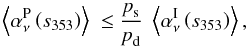 (30)where
 and
and
 are the mean SEDs of the synchrotron
emission correlated with dust in intensity and polarization. The upper limit in Eq.
(30) is obtained when the synchrotron
and dust polarization angles are identical, which is not what is observed comparing the
Planck353 GHz and WMAP 23 GHz polarization data (Planck
Collaboration Int. XIX 2015). Both emission processes trace the same
large-scale Galactic magnetic field (GMF), but they give different weights to different
parts of the line of sight. The CC analysis only keeps the synchrotron emission that
arises from the same volume of interstellar space as the dust emission. For example, it
is expected to filter out the synchrotron emission from the Galactic halo, where there
is little dust. Thus, to validate our interpretation of the low frequency rise of the
polarization SED with synchrotron and no AME polarization, we need to show that the
upper limit in Eq. (30) holds.
are the mean SEDs of the synchrotron
emission correlated with dust in intensity and polarization. The upper limit in Eq.
(30) is obtained when the synchrotron
and dust polarization angles are identical, which is not what is observed comparing the
Planck353 GHz and WMAP 23 GHz polarization data (Planck
Collaboration Int. XIX 2015). Both emission processes trace the same
large-scale Galactic magnetic field (GMF), but they give different weights to different
parts of the line of sight. The CC analysis only keeps the synchrotron emission that
arises from the same volume of interstellar space as the dust emission. For example, it
is expected to filter out the synchrotron emission from the Galactic halo, where there
is little dust. Thus, to validate our interpretation of the low frequency rise of the
polarization SED with synchrotron and no AME polarization, we need to show that the
upper limit in Eq. (30) holds.
The intrinsic polarization of synchrotron emission is about 75% for typical
relativistic electron spectra (Rybicki & Lightman
1979; Longair 1994), whereas the
analysis of Planck polarization maps indicates that the intrinsic
polarization of dust at 353 GHz can reach about 20% (Planck
Collaboration Int. XIX 2015; Planck
Collaboration Int. XX 2015). To compute the synchrotron SED in intensity,
, we combine the 353 GHz correlated CC coefficients,
corrected for the CMB (Sect. 5.3), obtained from
the fits with one and two templates (Sect. 4.2).
The SED of the synchrotron emission correlated with dust is then obtained by taking the
difference between the CC coefficients in Eqs. (8) and (11), and averaging over
all sky patches. It is shown in Fig. 10. We fit
this synchrotron SED with a power-law (PL) model. The normalized amplitude of
synchrotron emission at 23 GHz is  . This is the ratio between the 23 and
353 GHz emission in units of KRJ. The mean synchrotron spectral index derived from the
fit is
. This is the ratio between the 23 and
353 GHz emission in units of KRJ. The mean synchrotron spectral index derived from the
fit is  . The uncertainty on βs is
overestimated as the uncertainties on the synchrotron SED are highly correlated across
all WMAP and Planck frequencies. However, this is not critical for our
study because we do not use the uncertainty on βs in the
paper. The derived mean
. The uncertainty on βs is
overestimated as the uncertainties on the synchrotron SED are highly correlated across
all WMAP and Planck frequencies. However, this is not critical for our
study because we do not use the uncertainty on βs in the
paper. The derived mean  of the dust-correlated synchrotron
emission is consistent with the spectral index of 408-MHz-correlated synchrotron
emission obtained using WMAP data (Miville-Deschênes et
al. 2008; Dickinson et al. 2009; Gold et al. 2011; Ghosh et al. 2012), and the spectral index of the polarized synchrotron
emission (Fuskeland et al. 2014).
of the dust-correlated synchrotron
emission is consistent with the spectral index of 408-MHz-correlated synchrotron
emission obtained using WMAP data (Miville-Deschênes et
al. 2008; Dickinson et al. 2009; Gold et al. 2011; Ghosh et al. 2012), and the spectral index of the polarized synchrotron
emission (Fuskeland et al. 2014).
Using  , we find the theoretical upper limit on
 to be
to be
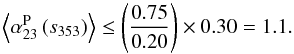 (31)The measured value of
![Mathematical equation: \hbox{$\langle[\tildealphaPnu]_{353}^{\rm 1T}\rangle$}](/articles/aa/full_html/2015/04/aa24088-14/aa24088-14-eq230.png) is 0.95 (shown in Fig. 11), which is within the upper limit. The difference
between the measured and theoretical upper limit in Eq. (30) can be explained by the fact that polarization angles traced by
synchrotron and dust emission are not perfectly aligned. We point out that that this
statement refers to the synchrotron emission correlated with the dust template in
intensity, which is not one to one correlated with dust in polarization.
is 0.95 (shown in Fig. 11), which is within the upper limit. The difference
between the measured and theoretical upper limit in Eq. (30) can be explained by the fact that polarization angles traced by
synchrotron and dust emission are not perfectly aligned. We point out that that this
statement refers to the synchrotron emission correlated with the dust template in
intensity, which is not one to one correlated with dust in polarization.
9.2.2. Upper limit on AME polarization
We can set an upper limit on the polarization fraction of AME by assuming that the synchrotron and dust polarization are totally uncorrelated. Within this hypothesis, the low frequency rise of the polarization SED is entirely due to polarized AME. Since both AME and thermal dust emission are associated with interstellar matter, it is reasonable to assume that the polarization angles are the same for AME and dust. We obtain the 353 GHz correlated AME polarization at 23 GHz as,
![Mathematical equation: \begin{eqnarray} &&\left\langle \left[\tilde{\alpha}_{23}^{\rm P}\right]_{353}^{\rm 1T}\right\rangle = \left\langle \alpha_{23}^{\rm P}\left(a_{353}\right) \right\rangle = \frac{\polfrac_{\rm a}}{\polfrac_{\rm d}} \left\langle \alpha_{23}^{\rm I}\left(a_{353}\right) \right\rangle , \nonumber \\ &&\text{i.e.,} \ \ 0.95 = \frac{\polfrac_{\rm a}}{\polfrac_{\rm d}} \left\langle \alpha_{23}^{\rm I}\left(a_{353}\right) \right\rangle , \nonumber\\ && \text{so} \ \ \polfrac_{\rm a}= \frac{\polfrac_{\rm d} \times 0.95} {\left\langle \alpha_{23}^{\rm I}\left(a_{353}\right) \right\rangle} \nonumber \\ &&\qquad = \frac{\polfrac_{\rm d} \times 0.95} {A_{\rm a}^{\rm I}} \cdot \hspace{0.4cm} \end{eqnarray}](/articles/aa/full_html/2015/04/aa24088-14/aa24088-14-eq249.png) (32)We use the mean AME amplitude,
(32)We use the mean AME amplitude,
 , from model DI+AI and Table 4, together with pd = 20%
(Planck Collaboration Int. XIX 2015; Planck Collaboration Int. XX 2015), to derive an
upper limit on the intrinsic polarization fraction of AME of about 16%. This is much higher than upper limits
reported from the analysis of compact sources (Dickinson
et al. 2011; López-Caraballo et al.
2011; Rubiño-Martín et al. 2012) and
theoretical predictions (Lazarian & Draine
2000; Hoang et al. 2013). Thus AME is
unlikely to be the sole explanation for the low frequency rise of the polarization SED,
even if we cannot exclude some contribution from AME.
, from model DI+AI and Table 4, together with pd = 20%
(Planck Collaboration Int. XIX 2015; Planck Collaboration Int. XX 2015), to derive an
upper limit on the intrinsic polarization fraction of AME of about 16%. This is much higher than upper limits
reported from the analysis of compact sources (Dickinson
et al. 2011; López-Caraballo et al.
2011; Rubiño-Martín et al. 2012) and
theoretical predictions (Lazarian & Draine
2000; Hoang et al. 2013). Thus AME is
unlikely to be the sole explanation for the low frequency rise of the polarization SED,
even if we cannot exclude some contribution from AME.
9.3. Parametric modelling for polarized dust SED
In this section we present a spectral model that fits the observed polarization SED. We
model the polarization SED with a combination of polarized synchrotron and dust
components. This model does not include AME. We account for the rise of the SED towards
the lowest frequencies with the synchrotron component. For the synchrotron component we
use the PL model with two parameters: the amplitude; and the spectral index. The PL model
of synchrotron emission is related to the power-law energy distribution of the cosmic-ray
electron spectrum (Abdo et al. 2009; Ackermann et al. 2010, 2012). The model is the superposition of a power-law synchrotron spectrum and
the MBB for the thermal dust emission. We refer to this model as PSI+PDI. It is described
by the equation: ![Mathematical equation: \begin{eqnarray} \left\langle \left[\tildealphaPnu\right]_{353}^{\rm 1T}\right\rangle& =& \ \AsP\ \left( \frac{\nu}{\nub}\right)^{\beta_{\rm s}^{\rm P}} + \left(\frac{\nu}{\nuref}\right)^{\beta_{\rm d,mm}^{\rm P} - 2} \frac{B_{\nu} (\Td)}{B_{\nuref} (\Td)} , \label{eq:9.3} \end{eqnarray}](/articles/aa/full_html/2015/04/aa24088-14/aa24088-14-eq253.png) (33)where
(33)where  is the amplitude of polarized synchrotron
components in KRJ
units, and is the polarized dust spectral index. The
polarized dust SED, expressed in KRJ units, is normalized to 1 at 353 GHz. Like for the two
intensity models, we fix Td = 19.6 K. We fit three parameters:
the synchrotron amplitude, the synchrotron and dust spectral index. We also fit this model
with an additional constraint that the spectral index of 353 GHz correlated synchrotron component is
the same for intensity and polarization. By doing so we have one less parameter to fit and
increase the number of degrees of freedom by one.
is the amplitude of polarized synchrotron
components in KRJ
units, and is the polarized dust spectral index. The
polarized dust SED, expressed in KRJ units, is normalized to 1 at 353 GHz. Like for the two
intensity models, we fix Td = 19.6 K. We fit three parameters:
the synchrotron amplitude, the synchrotron and dust spectral index. We also fit this model
with an additional constraint that the spectral index of 353 GHz correlated synchrotron component is
the same for intensity and polarization. By doing so we have one less parameter to fit and
increase the number of degrees of freedom by one.
The fits to the polarization SED for model with and without the constraint on
 are shown in Fig. 11. The parameters for the best-fit models are listed in Table 7. The two models provide very similar fits to the
observed polarized SED. If we force the spectral indices of the synchrotron for intensity
and polarization to be equal, we find an equally good fit to the polarization SED. These
results are further discussed in the next section.
are shown in Fig. 11. The parameters for the best-fit models are listed in Table 7. The two models provide very similar fits to the
observed polarized SED. If we force the spectral indices of the synchrotron for intensity
and polarization to be equal, we find an equally good fit to the polarization SED. These
results are further discussed in the next section.
Results of the spectral fits to the mean polarized dust SED obtained using Planck and WMAP data.
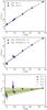 |
Fig. 12 Frequency dependence of the dust SED in intensity without AME (top), in polarization without synchrotron (middle), and the polarization fraction (bottom) for the four different combinations of dust models. The SEDs are plotted in units of KRJ and normalized to 1 at 353 GHz. The shaded areas represent 1σ (green), 2σ (yellow), and 3σ (grey) statistical uncertainty on the mean normalized polarization fraction. We used the mean spectra from the same 400 sky patches for both the intensity and polarization analysis. |
10. Comparison of the dust SEDs for intensity and polarization
We now compare the dust SEDs for intensity and polarization and discuss the frequency dependence of the polarization fraction within the context of existing dust models.
10.1. Spectral dependence of the polarization fraction
Figure 12 presents the dust SEDs for intensity and polarization derived from the spectral decomposition in emission components (Sects. 7.2 and 9.3). The SED for intensity, obtained after AME subtraction, is shown in the top panel of Fig. 12 from 70 to 353 GHz. The two sets of data points computed for each of the two AME models are very close to each other. The dust SED for polarization, obtained after subtraction of the synchrotron component, is shown in the middle panel of Fig. 12. The data points are plotted for the two spectral indices in Table 7, which differ by 0.4. The small difference between the corresponding points shows that the subtraction of the synchrotron component has a very small impact on the dust polarization SED even at 70 GHz. This indicates that our dust polarization SED is robust with respect to uncertainties on the spectral index of polarized synchrotron, including a possible steepening of the spectrum with increasing frequencies as discussed in Gold et al. (2011). The polarization fraction, shown in the bottom panel of Fig. 12, is normalized with respect to the data point at 353 GHz. The uncertainties on p include the uncertainties from both P and I. The data suggest that there is a small decrease in p by 21 ± 6% from 353 to 70 GHz.
10.2. The contribution of carbon dust and silicates to polarization
The results of this work set new observational constraints on dust models including silicate and carbon grains with possibly different polarization properties (Hildebrand et al. 1999; Martin 2007). We discuss the spectral dependence of p using the models from Draine & Li (2007), Compiègne et al. (2011), and Jones et al. (2013). In these three models, the thermal dust emission is the electric dipole emission from two types of grains, silicates and carbon grains, with distinct optical properties and thereby temperatures. The first two models use the same optical properties for silicates, but distinct properties for carbon grains; Draine & Li (2007) use the optical properties of graphite, while Compiègne et al. (2011) use results from laboratory measurements of amorphous carbon. The spectral index for carbon grains is 2 in the Draine & Li (2007) model and 1.6 in Compiègne et al. (2011). Over microwave frequencies, the opacity of silicates scales as ν1.6 in both models. Jones et al. (2013) use optical properties of amorphous carbon grains, which depend on the hydrogen fraction and degree of aromatization (Jones 2012). The spectral index of the carbon dust at 353 GHz varies between 1.2 and 2.3, depending on the nature of the carbon grains (see Fig. 14 of Jones et al. 2013, for more details).
SEDs from the first two models have been compared to the Planck dust SED in intensity in Planck Collaboration Int. XVII (2014) and Planck Collaboration Int. XXIX (2014). The differences between the model and the data are within 5–15% at ν< 353 GHz. Draine & Fraisse (2009) have used the Draine & Li (2007) dust model to compute spectra for dust polarization. They predict a systematic increase of the polarization fraction p at microwave frequencies when only silicates contribute to dust polarization. This prediction is not what we report in this paper. However, model predictions for the spectral dependency of p are related to the difference in spectral index between carbon and silicate grains, which is not known. Thus, a difference between carbon and silicate polarization may be the correct physical interpretation of the spectral dependence of p, even if the data do not match the Draine & Fraisse (2009) model.
Calculations of the polarized SED for the Compiègne et al. (2011) and Jones et al. (2013) models are needed to assess quantitatively this interpretation. In the Compiègne et al. (2011) model, the spectra from silicates and carbon grains are very similar at long wavelengths and we do not expect p to depend on wavelength when only silicates contribute to the polarization. In the Jones et al. (2013) model the contribution from carbon dust grains could be dominant at ν< 353 GHz.
10.3. Microwave dust emission
The dust SED in polarization and the spectral dependence of p allows us to discuss two possible interpretations of the dust microwave emission.
Meny et al. (2007) introduced a physical
description of FIR/microwave dust emission, where the microwave dust opacity of amorphous
grains is dominated by low energy transitions associated with disorder in the structure of
the solids on atomic scales. This contribution is modelled by transitions in two-level
systems (TLS). The TLS model is supported by experimental results on silicates (Agladze et al. 1996; Boudet et al. 2005; Coupeaud et al.
2011), which indicate that the opacity of amorphous silicate grains flattens
towards long wavelengths. The TLS model has been used to model dust emission spectra by
Paradis et al. (2011). It was also proposed as a
possible interpretation of the flattening of the dust SED in intensity from FIR to mm
wavelengths, which was reported in two earlier Planck papers on the diffuse dust emission
in the Galactic plane in Planck Collaboration Int. XIV
(2014) and at high Galactic latitudes in Planck
Collaboration Int. XVII (2014). Our analysis based on new Planck
data does not confirm this flattening, but does not dismiss it either because the
error-bars on the submm spectral index from calibration uncertainties remain significant:
0.16 (1σ)
from Sect. 5.2. Within the TLS model, a flattening
of the dust SED in intensity would be due to a decrease in the spectral index of silicate
grains at long wavelengths. Since silicate grains are polarized, the flattening of the
dust SED should also be seen in polarization. This expectation is not supported by the
results of our data analysis, namely the difference in spectral indices of the thermal
dust emission in intensity and polarization ( and
) reported in Sect. 8.2.
MDE has been introduced by Draine & Hensley (2012) to explain the flattening of the dust SED at sub-mm wavelengths in the Small Magellanic Cloud (Planck Collaboration XVII 2011). MDE could also contribute to the long wavelength emission of Galactic dust. Model spectra of MDE are presented in Draine & Hensley (2013) for Galactic dust. The contribution of MDE could be significant at frequencies smaller than a few hundred GHz and increasing towards smaller frequencies. If the magnetic particles are inclusions randomly-oriented within interstellar grains, their emission is polarized in a direction perpendicular to that of the dipolar electric emission (Draine & Hensley 2013). In this case, we expect this emission component to reduce the polarization of the dust emission. This could possibly account for the observed decrease in p from 353 to 70 GHz.
A fit of the SEDs in polarization and intensity with the models of Paradis et al. (2011) and Draine & Hensley (2013) would be necessary to test these two interpretations quantitatively.
11. Conclusion
We have characterized the frequency dependence of dust emission in intensity and polarization by analysing Planck data over 39% of the sky at intermediate Galactic latitudes. We use the Planck353 GHz I, Q, and U maps as templates for dust emission in intensity and polarization. We cross-correlate them with the Planck and WMAP data, at 12 frequencies from 23 to 353 GHz. The main results of the data analysis are as follows.
-
The mean spectral index of the dust emission measured between 100 and 353 GHz is
 . This value agrees with that reported
by Planck Collaboration Int. XVII (2014) for
the high Galactic latitude sky and Planck
Collaboration Int. XIV (2014) for diffuse emission in the Galactic plane. The
microwave spectral index is close to that at submm wavelengths,
which is derived from fits to the Planck data at ν ≥ 353 GHz with the
full-mission Planck data.
. This value agrees with that reported
by Planck Collaboration Int. XVII (2014) for
the high Galactic latitude sky and Planck
Collaboration Int. XIV (2014) for diffuse emission in the Galactic plane. The
microwave spectral index is close to that at submm wavelengths,
which is derived from fits to the Planck data at ν ≥ 353 GHz with the
full-mission Planck data. -
We determine the mean dust SED in intensity from 23 to 353 GHz. We separate the dust and AME contributions to the SED. The dust contribution is well fit by combining the modified blackbody spectrum with a spectral index of 1.51 with the mean temperature of 19.6 K. The two parametric models we use for the AME yield the same SED for the dust for frequencies ν ≥ 70 GHz.
-
The mean spectral index for dust polarization, measured between 100 and 353 GHz, is
 , assuming the temperature of aligned
dust grains contributing to the polarization is the same as that determined from the
dust emission in intensity. We show that the small difference with
, assuming the temperature of aligned
dust grains contributing to the polarization is the same as that determined from the
dust emission in intensity. We show that the small difference with
 , the spectral index measured in a
similar way for dust intensity, is a robust result against systematic uncertainties
estimated comparing results of our data analysis obtained on various subsets of the
Planck data.
, the spectral index measured in a
similar way for dust intensity, is a robust result against systematic uncertainties
estimated comparing results of our data analysis obtained on various subsets of the
Planck data. -
We determine the SED of the dust-correlated polarized emission from 23 to 353 GHz. This SED decreases with decreasing frequency and turns up below 60 GHz, very much like the dust SED in intensity due to AME. We show that the low frequency rise of the polarization SED may be explained by synchrotron polarization correlated with dust.
-
We use a parametric model to separate the synchrotron and dust polarization and to characterize the spectral dependence of the dust polarization fraction. The polarization fraction p of the dust emission decreases by (21 ± 6)% from 353 to 70 GHz. We discuss this result within the context of existing dust models. It could indicate differences in polarization efficiency among components of interstellar dust (e.g., carbon and silicate grains).
Our observational results provide inputs to quantify and optimize the separation between Galactic and CMB polarization (Planck Collaboration Int. XXX 2015). Our CC analysis yields a spectral decomposition of the diffuse emission into its main components: thermal emission from dust; free-free; synchrotron; and AME. This spectral decomposition may be combined with power spectra of the templates, as discussed in Appendix D, to quantify the Galactic emission in intensity as a function of the observed frequency and multipole (see Figs. 27 and 28 in Planck Collaboration I 2014). For polarization, we are currently missing a synchrotron polarization template that is free from Faraday rotation. Polarized synchrotron templates, which are expected from C-BASS (King et al. 2010) at 5 GHz and QUIJOTE (Hoyland et al. 2012) between 10 and 20 GHz, will be important for future correlation analyses.
Online material
Appendix A: Derivation of the CC coefficients
This appendix details how we compute the dust SED using the CC analysis in Sect. 4.2. For simplicity, we present the simplest case for intensity from the fit with one template.
We minimize the between the data and the 353 GHz template maps, as expressed in Eq.
(7). The CC coefficient is then given
as ![Mathematical equation: \appendix \setcounter{section}{1} \begin{equation} \left[\alphaInu\right]_{353}^{\rm 1T} = \frac{\sum_{k=1}^{N_{\rm pix}} \hat{\nI}(k) \ . \ \hatI_{353}(k)}{ \sum_{k=1}^{N_{\rm pix}} \ \hatI_{353}(k)^2} , \label{eq:a1.2} \end{equation}](/articles/aa/full_html/2015/04/aa24088-14/aa24088-14-eq270.png) (A.1)where
(A.1)where
 and Î353 are the
data and 353 GHz template
with mean values (computed over the Npix) subtracted. The observed
Planck map at a given frequency is written as the sum of the CMB
signal, the Galactic signals (synchrotron, free-free, dust and AME) and noise as
and Î353 are the
data and 353 GHz template
with mean values (computed over the Npix) subtracted. The observed
Planck map at a given frequency is written as the sum of the CMB
signal, the Galactic signals (synchrotron, free-free, dust and AME) and noise as
 (A.2)where the superscripts c, d, s, f, e, and n
represent the CMB, dust, synchrotron, free-free, AME, and noise, respectively. Combining
Eqs. (A.1) and (A.2) we find
(A.2)where the superscripts c, d, s, f, e, and n
represent the CMB, dust, synchrotron, free-free, AME, and noise, respectively. Combining
Eqs. (A.1) and (A.2) we find ![Mathematical equation: \appendix \setcounter{section}{1} \begin{eqnarray} &&\left[\alphaInu\right]_{353}^{\rm 1T} = N \sum_{k=1}^{N_{\rm pix}} \left[ \hatI^{\rm c} (k) + \hatI^{\rm d}_{\nu} (k) + \hatI^{\rm s}_{\nu} (k) + \hatI^{\rm f}_{\nu} (k) + \hatI^{\rm e}_{\nu} (k) + \hatI^{\rm n}_{\nu} (k) \right] \nonumber \\ && \times \left[ \hatI^{\rm c} (k) + \hatI^{\rm d}_{353} (k) + \hatI^{\rm s}_{353} (k) + \hatI^{\rm f}_{353} (k) + \hatI^{\rm e}_{353} (k) + \hatI^{\rm n}_{353} (k) \right] \label{eq:a1.4} , \end{eqnarray}](/articles/aa/full_html/2015/04/aa24088-14/aa24088-14-eq275.png) (A.3)where
(A.3)where
 is the normalization factor. At HFI
frequencies, we can neglect the contribution of the synchrotron, free-free, AME, and
noise within our global mask. This reduces Eq. (A.3) to
is the normalization factor. At HFI
frequencies, we can neglect the contribution of the synchrotron, free-free, AME, and
noise within our global mask. This reduces Eq. (A.3) to ![Mathematical equation: \appendix \setcounter{section}{1} \begin{eqnarray} \left[\alphaInu\right]_{353}^{\rm 1T}& = &N \sum_{k=1}^{N_{\rm pix}} \ \left ( \hatI^{\rm c} (k) + \hatI^{\rm d}_{\nu} (k) \right ) \ \times \ \left( \hatI^{\rm c} (k) + \hatI^{\rm d}_{353} (k) \right ) \nonumber \\ & =& N \ \sum_{k=1}^{N_{\rm pix}} \left [ \ \hatI^{\rm c} (k) \left ( \hatI^{\rm c} (k) + \hatI^{\rm d}_{353} (k) \right ) + \ \hatI^{\rm d}_{\nu} (k) \left ( \hatI^{\rm c} (k) + \hatI^{\rm d}_{353} (k) \right ) \right ] \nonumber \\ & = &\alpha\left(c_{353}\right ) + N \sum_{k=1}^{N_{\rm pix}} \hatI^{\rm d}_{\nu} (k) \left ( \hatI^{\rm c} (k) + \hatI^{\rm d}_{353} (k) \right ) . \end{eqnarray}](/articles/aa/full_html/2015/04/aa24088-14/aa24088-14-eq277.png) (A.4)The CMB contribution, α(c353), is the CC
coefficient obtained by correlating the CMB signal map with the 353 GHz template, which is independent of
frequency. The dust emission at a given frequency is a scaled version of 353 GHz dust emission,
(A.4)The CMB contribution, α(c353), is the CC
coefficient obtained by correlating the CMB signal map with the 353 GHz template, which is independent of
frequency. The dust emission at a given frequency is a scaled version of 353 GHz dust emission,
 , where
 is the mean dust SED over the given sky
patch. The CC coefficient is then
is the mean dust SED over the given sky
patch. The CC coefficient is then ![Mathematical equation: \appendix \setcounter{section}{1} \begin{eqnarray} \left[\alphaInu\right]_{353}^{\rm 1T}& = &\alpha\left(c_{353}\right) + \alpha^{\rm d}_{\nu} \ N \sum_{k=1}^{N_{\rm pix}} \hatI^{\rm d}_{353} (k) \left ( \hatI^{\rm c} (k) + \hatI^{\rm d}_{353} (k) \right ) \nonumber \\ & = &\alpha(c_{353}) + \alphaInu \left(d_{353}\right) . \label{eq:a1.5} \end{eqnarray}](/articles/aa/full_html/2015/04/aa24088-14/aa24088-14-eq281.png) (A.5)where
(A.5)where
 is proportional to the mean dust SED.
The colour ratio is then given by
is proportional to the mean dust SED.
The colour ratio is then given by ![Mathematical equation: \appendix \setcounter{section}{1} \begin{eqnarray} \label{eq:a1.6} R^{\rm I}_{100}(353,217)& = &\dfrac{\left[\alpha^{\rm I}_{353}\right]_{353}^{\rm 1T} -\left[\alpha^{\rm I}_{100}\right]_{353}^{\rm 1T} }{\left[\alpha^{\rm I}_{217}\right]_{353}^{\rm 1T} -\left[\alpha^{\rm I}_{100}\right]_{353}^{\rm 1T} } = \dfrac{\alpha^{\rm d}_{353} - \alpha^{\rm d}_{100} }{\alpha^{\rm d}_{217} - \alpha^{\rm d}_{100}} \cdot \end{eqnarray}](/articles/aa/full_html/2015/04/aa24088-14/aa24088-14-eq283.png) (A.6)In the ratio the scaling between the
and
goes away. The colour ratio only depends
on the dust spectral properties and not on the CMB signal. The extension of Eq. (A.5) in the presence of AME, synchrotron,
and free-free emission at the WMAP and LFI frequencies is given by Eq. (8).
(A.6)In the ratio the scaling between the
and
goes away. The colour ratio only depends
on the dust spectral properties and not on the CMB signal. The extension of Eq. (A.5) in the presence of AME, synchrotron,
and free-free emission at the WMAP and LFI frequencies is given by Eq. (8).
The CMB contribution, α(c353), in the
presence of inverse noise-weighting can be written as
 (A.7)where wν is a weighting
factor given by
(A.7)where wν is a weighting
factor given by  . If the weighting factor depends on the
frequency, the CMB contribution is not strictly constant in KCMB units. This effect can
reach up to 2%, as the weighting factors for the WMAP and Planck maps
are quite different. This is not negligible compared to the dust emission at microwave
frequencies. That is the reason why we do not use inverse noise-weighting in our
minimization.
. If the weighting factor depends on the
frequency, the CMB contribution is not strictly constant in KCMB units. This effect can
reach up to 2%, as the weighting factors for the WMAP and Planck maps
are quite different. This is not negligible compared to the dust emission at microwave
frequencies. That is the reason why we do not use inverse noise-weighting in our
minimization.
In Sect. 9.2.1 we compute the frequency
dependence of synchrotron emission correlated with dust. The mean spectrum of this
component is given by  (A.8)assuming the CMB chance correlation term
with synchrotron emission is zero over all the sky patches. We detect
with high-significance in our analysis
(Sect. 9.2.1), which cannot be just a chance
correlation term. One would expect such a correlation, since synchrotron emission arises
from the same ISM as dust emission.
(A.8)assuming the CMB chance correlation term
with synchrotron emission is zero over all the sky patches. We detect
with high-significance in our analysis
(Sect. 9.2.1), which cannot be just a chance
correlation term. One would expect such a correlation, since synchrotron emission arises
from the same ISM as dust emission.
Similarly for polarization, we minimize between the data and 353 GHz Stokes Q and U maps, as given by Eq.
(13). The polarization CC coefficient
is then given by ![Mathematical equation: \appendix \setcounter{section}{1} \begin{equation} \left[\alphaPnu\right]_{353}^{\rm 1T} = N_{\rm P} \sum_{i=1}^2 \ \sum_{k=1}^{N_{\rm pix}} \left [ \hatQ_{\nu}(k) \ . \ \hatQ^i_{353}(k) + \hatU_{\nu}(k) \ . \ \hatU^i_{353}(k) \right ] , \label{eq:a1.7} \end{equation}](/articles/aa/full_html/2015/04/aa24088-14/aa24088-14-eq288.png) (A.9)where NP is the
normalization factor for polarization. Following the same logic as described for
intensity, the polarization CC coefficient at the HFI frequencies can be written as
(A.9)where NP is the
normalization factor for polarization. Following the same logic as described for
intensity, the polarization CC coefficient at the HFI frequencies can be written as
![Mathematical equation: \appendix \setcounter{section}{1} \begin{eqnarray} \left[\alphaPnu\right]_{353}^{\rm 1T} &=& \alpha^{\rm P}(c_{353}) \nonumber \\ & &+ \ N_{\rm P} \sum_{i=1}^2 \ \sum_{k=1}^{N_{\rm pix}} \left [ \hatQ^{\rm d}_{\nu}(k) \ \left ( \hatQ^{\rm c} (k) + \hatQ^{\rm d}_{353}(k) + \hatQ_{353}^{\rm {n}_i} (k) \right ) \right ] \nonumber \\ \label{eq:a.1.8} && +\ N_{\rm P} \sum_{i=1}^2 \ \sum_{k=1}^{N_{\rm pix}} \left [ \hatU^{\rm d}_{\nu}(k) \ \left ( \hatU^{\rm c} (k) + \hatU^{\rm d}_{353}(k) + \hatU_{353}^{\rm {n}_i} (k) \right ) \right ]. \end{eqnarray}](/articles/aa/full_html/2015/04/aa24088-14/aa24088-14-eq290.png) (A.10)
(A.10)
Assuming the dust polarization at a given frequency is a scaled version of
353 GHz dust polarization
yields  and
and
 . Putting this back to into Eq. (A.10) gives
![Mathematical equation: \appendix \setcounter{section}{1} \begin{equation} \left[\alphaPnu\right]_{353}^{\rm 1T} =\alpha^{\rm P}\left(c_{353}\right) + \alphaPnu\left(d_{353}\right) . \end{equation}](/articles/aa/full_html/2015/04/aa24088-14/aa24088-14-eq293.png) (A.11)The polarized colour ratio does not depend
on the CMB like Eq. (A.5). The polarized
CMB contribution αP(c353)
is strictly constant in KCMB units if we do not apply any noise weighting,
similar to the intensity analysis. To deal with the noise, we first smooth all the maps
to 1° resolution and then
perform correlation over local patches on the sky. To compute the uncertainty on the CC
coefficients, we rely on Monte Carlo simulations, as discussed in Appendix B.
(A.11)The polarized colour ratio does not depend
on the CMB like Eq. (A.5). The polarized
CMB contribution αP(c353)
is strictly constant in KCMB units if we do not apply any noise weighting,
similar to the intensity analysis. To deal with the noise, we first smooth all the maps
to 1° resolution and then
perform correlation over local patches on the sky. To compute the uncertainty on the CC
coefficients, we rely on Monte Carlo simulations, as discussed in Appendix B.
Appendix B: Simulations
This appendix presents the simulations of the sky emission in intensity and polarization at HFI frequencies that we use to test the CC analysis. The intensity and polarization emission components are listed in Table B.1. The simulations use a simplified model of dust emission in intensity and polarization that is good enough to provide a realistic framework to test the CC analysis. They are computed on HEALPix pixels at Nside = 128 with a 1° Gaussian beam. The Monte Carlo simulations serve two specific purposes. First, we use them to check that the CC analysis does not introduce any bias on our estimations of the mean dust spectral indices in intensity and polarization. Second, they provide realistic uncertainties on the CC coefficients, which we use in the spectral fit to separate out the dust and the CMB emission (Sect. 5.3).
The ancillary data sets and models used in the Monte Carlo simulations.
Appendix B.1: Intensity
At HFI frequencies, the main diffuse emission components are the thermal dust, free-free, CMB, and CIB emission. The simulations also include instrumental noise. We now describe how we simulate each of these components.
The Hi column density from the LAB survey (Kalberla et al. 2005) is taken as a proxy for thermal dust emission. We
normalize the Hi data to a suitable amplitude to match the observed
Planck data at 353 GHz and extrapolate to the other HFI frequencies using an MBB
spectrum with a fixed spectral index βd = 1.5 and temperature
Td =
19.6 K over the whole sky. The Hi data provide only a
partial description of the thermal dust emission, as quoted in Planck Collaboration Int. XVII (2014). We include an additional
dust component, spatially uncorrelated with the Hi data, to mimic the
residuals present after adopting the IR-Hi correlation at 857 GHz. The
additional dust-like emission is assumed to have an ℓ-3 power
spectrum, with a normalized amplitude of  for ℓ = 2, where
σ857 is the residual at 857 GHz after
applying the IR-Hi correlation and removing the CIB contribution (Planck Collaboration Int. XVII 2014). The amplitude
of the uncorrelated Hi emission is normalized at 857 GHz, taken from Planck Collaboration Int. XVII (2014), and scaled
to the HFI frequencies assuming βR = 2.0 for a dust temperature of
TR =
19.6 K. We use the DDD Hα map as a proxy for free-free emission, which
we compute at HFI frequencies for a spectral index βf = −2.14
(in KRJ units;
Planck Collaboration Int. XIV 2014) and an
electron temperature Te = 7000 K (Dickinson et al. 2003). No dust extinction correction is applied to
the DDD Hα map.
for ℓ = 2, where
σ857 is the residual at 857 GHz after
applying the IR-Hi correlation and removing the CIB contribution (Planck Collaboration Int. XVII 2014). The amplitude
of the uncorrelated Hi emission is normalized at 857 GHz, taken from Planck Collaboration Int. XVII (2014), and scaled
to the HFI frequencies assuming βR = 2.0 for a dust temperature of
TR =
19.6 K. We use the DDD Hα map as a proxy for free-free emission, which
we compute at HFI frequencies for a spectral index βf = −2.14
(in KRJ units;
Planck Collaboration Int. XIV 2014) and an
electron temperature Te = 7000 K (Dickinson et al. 2003). No dust extinction correction is applied to
the DDD Hα map.
For the CMB, we compute Gaussian realizations of the CMB sky from the theoretical power spectrum of the Planck best-fit model (Planck Collaboration XV 2014). The CIB emission is generated using the best-fit model of CIB anisotropies at 353 GHz obtained directly from the Planck data (Planck Collaboration XXX 2014). We assume 100% correlated CIB across all the HFI frequencies, assuming an MBB spectrum with βCIB = 1.3 and TCIB = 18.4 K. The Gaussian realizations of the instrumental noise are obtained at each frequency, using the noise variance maps (Planck Collaboration VI 2014). The noise realizations are simulated at the full resolution of the Planck data, before smoothing to 1° resolution and reducing the pixelization from Nside = 2048 to 128.
We compute 1000 realizations of sky maps of the additional dust component, together with the CMB and CIB anisotropies. Independent realizations of the instrumental noise are generated for each sky simulation at a given frequency. The dust component computed from the Hi map and the free-free emission traced by the Hα map are kept fixed.
We analyse the 1000 simulated maps with the CC method applied to the
Planck intensity data. We compute the mean and standard deviation
of the values for each sky patch. Both are
plotted in Fig. B.1 versus the local dispersion
of the 353 GHz template,
. There is no bias on the estimation of
the mean dust spectral index . We recover a mean value equal to the
index of 1.5 we used for the main Hi-correlated dust component. The
uncertainties on , and hence on
, are associated with noise, CIB
anisotropies, free-free emission, and the additional dust component. The
1σ
dispersion of across sky patches for a given Monte
Carlo realization is 0.02. This is smaller than the scatter of 0.07 measured for the
Planck data. We interpret the difference as evidence for a small
intrinsic dispersion in the spectral index of the dust emission.
Appendix B.2: Polarization
The simulations of the polarized sky at HFI frequencies include polarized CMB, thermal dust emission, and noise. We compute 1000 realizations of the CMB Stokes Q and U maps using the best-fit Planck model (Planck Collaboration XV 2014), smoothed to 1° resolution at HEALPix resolution Nside = 128. Random realizations of Gaussian noise Q and U maps are generated at each pixel using the 3 × 3 noise covariance matrix defined at Nside = 2048. The noise maps are then smoothed to 1° resolution and projected on to a HEALPix map at Nside = 128. We generate independent realizations of the instrumental noise to mimic the detector sets at 353 GHz (Sect. 2.1.2).
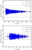 |
Fig. B.1 R100(353,217) colour ratios from the Monte Carlo simulations for intensity (top) and polarization (bottom). The two plots show that the CC analysis does not introduce any bias on the estimation of βd,mm. |
For polarized thermal dust emission, we use the following model:
![Mathematical equation: \appendix \setcounter{section}{2} \begin{equation} \left[\StokesQ^{\rm d}_{\nu} , \StokesU^{\rm d}_{\nu}\right] = \polfrac_{\rm d} \left( \frac{\nu}{\nuref} \right)^{\beta_{\rm d,mm}^{\rm P}} \frac{B_{\nu}(\Td)}{B_{\nuref}(\Td)}\ I_{\nuref}^{\rm d} \ \left[\cos 2\polang_{\rm d} , \sin 2\polang_{\rm d}\right]. \end{equation}](/articles/aa/full_html/2015/04/aa24088-14/aa24088-14-eq319.png) (B.1)Here pd,
(B.1)Here pd,
 , and ψd are the
polarization fraction, the dust intensity at reference frequency, and the polarization
angle, respectively. The reference frequency is νref =
353 GHz. We fix pd to a constant value of 10% over
the whole sky. The map is that obtained by Planck Collaboration XI (2014) from the spectral
fit to the high frequency Planck and IRAS 100 μm data, with an
MBB model. For the dust polarization, we use an MBB spectrum with
, and ψd are the
polarization fraction, the dust intensity at reference frequency, and the polarization
angle, respectively. The reference frequency is νref =
353 GHz. We fix pd to a constant value of 10% over
the whole sky. The map is that obtained by Planck Collaboration XI (2014) from the spectral
fit to the high frequency Planck and IRAS 100 μm data, with an
MBB model. For the dust polarization, we use an MBB spectrum with
 and Td = 19.6 K,
constant over the whole sky. We derive ψd from the 1° smoothed Planck
Stokes maps using the relation
and Td = 19.6 K,
constant over the whole sky. We derive ψd from the 1° smoothed Planck
Stokes maps using the relation
 (B.2)We choose ν1 and
ν2 as the 143 and 353 GHz, respectively. The difference
between the two frequencies removes the CMB contribution.
(B.2)We choose ν1 and
ν2 as the 143 and 353 GHz, respectively. The difference
between the two frequencies removes the CMB contribution.
We analyse 1000 polarized simulated maps using the CC analysis as applied to the
Planck data. We compute the mean and the standard deviation of the
for each sky patch. The plot of
versus
is shown in Fig. B.1. We find no bias in the estimation of
and hence in the measurement of
. The 1σ dispersion of
across sky patches for a given
simulation is 0.07. The 1σ dispersion of
from the simulations is smaller
compared than that measured from the Planck data, because we use a
simplified white noise model. However, some of the dispersion may come from the
intrinsic dispersion of the polarized dust spectral index, and also additional
Galactic polarized emission components, which we neglect in the simulations.
Appendix C: Mean dust SED with dust extinction and scattering correction on the Hα template
The mean dust SED for intensity presented in this paper is obtained using the three-template fit with no extinction and dust scattering correction from the DDD Hα template. The effect of dust extinction (fd) on the Hα template is described in Eq. (3) of Dickinson et al. (2003), whereas the effect of dust scattering (sd) on the Hα template is described in Eq. (26) of Bennett et al. (2013). The mean measured value of sd is 0.11 R( MJy sr-1)-1 in high Galactic latitude regions (Lehtinen et al. 2010; Witt et al. 2010; Seon & Witt 2012; Brandt & Draine 2012; Bennett et al. 2013). To check the impact of the fd and sd corrected Hα template on the mean dust SED, we repeat the analysis with different combinations of fd and sd. The three different combinations of fd and sd corrected Hα templates we choose are: fd = 0.3 and sd = 0.0 R( MJy sr-1)-1; fd = 0.0 and sd = 0.11 R( MJy sr-1)-1; and fd = 0.3 and sd = 0.11 R( MJy sr-1)-1. The fractional change in the mean dust SED with respect to the reference dust SED (fd = 0.0 and sd = 0.0 R( MJy sr-1)-1) is presented in Fig. C.1. At higher frequencies (ν ≥ 100 GHz), the impact of both dust extinction and scattering is negligible. However at frequencies ν ≤ 50 GHz, the fractional change on the mean SED can go as high as ±4%. The fd and sd parameters are degenerate, although their effect on the derived best-fit parameter of models DI+AI and DI+AII, listed in Table 4, is very small.
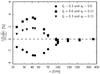 |
Fig. C.1 Fractional change in the mean dust SED with respect to the reference dust SED presented in this paper, for different combinations of fd and sd corrections on the DDD Hα template. |
Appendix D: Power spectra of the templates
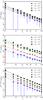 |
Fig. D.1 Power spectra of the 408 MHz, DDD Hα, and SMICAsubtracted 353 GHz templates, smoothed to 1° resolution for different Galactic masks (or fsky). |
In this section, we compute the temperature power spectra of the three templates at 1° resolution: 408 MHz; DDD Hα; and 353 GHz dust template. The Planck353 GHz map contains a significant component of CMB anisotropies. Taking the SMICA map (Planck Collaboration XII 2014) as a proxy for the CMB map, we remove its contribution from the 353 GHz total map. These spectra are combined with the SEDs from this paper to compute the contributions of each emission component to the microwave sky emission as a function of angular scales in Planck Collaboration I (2014, see their Figs. 27 and 28).
For the computation of the power spectra, we consider the four diffuse Galactic masks based on the percentage of the sky retained (fsky), i.e., G40, G60, G70 and G80 (Planck Collaboration XV 2014). The same set of masks have been used in the likelihood analysis of the 2013 Planck data release (Planck Collaboration XV 2014). The power spectra are computed only at low multipoles (ℓ< 100) with PolSpice v2.9.0 (Chon et al. 2004), corrected for the masking, beam, and pixel window effect. Figure D.1 presents binned power spectra of the three templates: 408 MHz, DDD Hα, and SMICA-subtracted 353 GHz maps as a function of the Galactic masks. The uncertainties on the binned power spectra include only the statistical variance and not the cosmic variance.
At low multipoles, ℓ< 100, the three power spectra are well-fit with a power-law model. Using this assumption, the measured power spectra are written as Cℓ = A × (ℓ/ 100)α. Here A represents the normalized amplitude at ℓ = 100 and α represents the slope of the power-law for a given template. We fix α based on the measured spectra and only fit for the amplitudes as a function of the Galactic masks. We find that the slope of the 408 MHz spectra over all the Galactic masks is consistent with − 2.5. In case of DDD Hα template is − 2.2 over the masks and the same for the SMICA-subtracted 353 GHz template is − 2.4. The results of the power-law fit for the three templates and different Galactic masks are shown as a dashed lines in Fig. D.1. The amplitudes of each of the templates as a function of the Galactic masks (or fsky) are listed in Table D.1.
Amplitudes of the power spectra, normalized at ℓ = 100, as a function of fsky.
The amplitudes of the given templates vary nonlinearly as a function of fsky. They can
be fitted with a second-order polynomial in a log A – log fsky plane.
Combining the ν, ℓ, and fsky dependence, we analytically model
the power spectra of the diffuse synchrotron, free-free, and dust emission components
for intensity. For amplitude normalization, we made an assumption on the nature of the
synchrotron and free-free emission. We assume a single power-law model for the
synchrotron emission from 408 MHz to microwave frequencies, ν ≤ 353 GHz. For
free-free emission, we assume a single power-law model at microwave frequencies, with a
mean electron temperature of 7000 K (Dickinson et al.
2003). The power spectra of the three diffuse emission components, in
 units, are
![Mathematical equation: \begin{eqnarray} \Cl^{\rm f} & =& \ 0.068 \times \left ( \frac{f_{\rm sky}}{0.6} \right)^{\left [6.10 \ + 3.90 \ln \left ({f_{\rm sky}/0.6} \right) \right ]} \nonumber \\[0.5mm] &&\times~ \left( \frac{\ell}{100}\right)^{-2.2} \times \left(\frac{\nu}{\nub}\right)^{-4.28}, \\[0.5mm] \Cl^{\rm s} & =& \ 2.96 \times 10^{9} \times \left ( \frac{f_{\rm sky}}{0.6} \right)^{\left [2.12 \ + 2.67 \ln \left ({f_{\rm sky}/0.6} \right) \right ]}\nonumber \\[0.5mm] &&\times~ \left( \frac{\ell}{100}\right)^{-2.5} \times \left( \frac{\nu}{\nuc}\right)^{-6.0}, \\[0.5mm] \Cl^{\rm d} & =& 0.086 \times \left ( \frac{f_{\rm sky}}{0.6} \right)^{\left [4.60 \ + 7.11 \ln \left ({f_{\rm sky}/0.6} \right) \right ]} \times \left( \frac{\ell}{100}\right)^{-2.4} \times \mathcal{D_{\nu}},\quad\quad\quad \end{eqnarray}](/articles/aa/full_html/2015/04/aa24088-14/aa24088-14-eq272.png) where νb = 23 GHz,
νc =
0.408 GHz,
where νb = 23 GHz,
νc =
0.408 GHz,  is a spectral model of the dust emission given by one of the two models presented in
Eqs. (26), and (27). The derived analytical model of these
power spectra are valid in the frequency range 20 to 353 GHz, and for fsky between
0.4 and 0.8.
is a spectral model of the dust emission given by one of the two models presented in
Eqs. (26), and (27). The derived analytical model of these
power spectra are valid in the frequency range 20 to 353 GHz, and for fsky between
0.4 and 0.8.
Planck (http://www.esa.int/Planck) is a project of the European Space Agency (ESA) with instruments provided by two scientific consortia funded by ESA member states (in particular the lead countries France and Italy), with contributions from NASA (USA) and telescope reflectors provided by a collaboration between ESA and a scientific consortium led and funded by Denmark.
These values are derived from a grey-body fit of dust SED at ν ≥ 353 GHz. The error-bar on the dust temperature is associated with that on the spectral index.
Acknowledgments
The Planck Collaboration acknowledges the support of: ESA; CNES and CNRS/INSU-IN2P3-INP (France); ASI, CNR, and INAF (Italy); NASA and DoE (USA); STFC and UKSA (UK); CSIC, MICINN and J.A. (Spain); Tekes, AoF and CSC (Finland); DLR and MPG (Germany); CSA (Canada); DTU Space (Denmark); SER/SSO (Switzerland); RCN (Norway); SFI (Ireland); FCT/MCTES (Portugal); and DEISA (EU). A detailed description of the Planck Collaboration and a list of its members can be found at http://www.rssd.esa.int/index.php?project=PLANCK&page=Planck_Collaboration. The research leading to these results has received funding from the European Research Council under the European Union’s Seventh Framework Programme (FP7/2007-2013)/ERC grant agreement No. 267934. We acknowledge the use of the Legacy Archive for Microwave Background Data Analysis (LAMBDA), part of the High Energy Astrophysics Science Archive Center (HEASARC). HEASARC/LAMBDA is a service of the Astrophysics Science Division at the NASA Goddard Space Flight Center. Some of the results in this paper have been derived using the HEALPix package.
References
- Abdo, A. A., Ackermann, M., Ajello, M., et al. 2009, Phys. Rev. Lett., 102, 181101 [NASA ADS] [CrossRef] [PubMed] [Google Scholar]
- Ackermann, M., Ajello, M., Atwood, W. B., et al. 2010, Phys. Rev. D, 82, 092004 [NASA ADS] [CrossRef] [Google Scholar]
- Ackermann, M., Ajello, M., Allafort, A., et al. 2012, Phys. Rev. Lett., 108, 011103 [NASA ADS] [CrossRef] [PubMed] [Google Scholar]
- Agladze, N. I., Sievers, A. J., Jones, S. A., Burlitch, J. M., & Beckwith, S. V. W. 1996, ApJ, 462, 1026 [NASA ADS] [CrossRef] [Google Scholar]
- Ali-Haïmoud, Y., Hirata, C. M., & Dickinson, C. 2009, MNRAS, 395, 1055 [NASA ADS] [CrossRef] [Google Scholar]
- Banday, A. J., Gorski, K. M., Bennett, C. L., et al. 1996, ApJ, 468, L85 [NASA ADS] [CrossRef] [Google Scholar]
- Banday, A. J., Dickinson, C., Davies, R. D., Davis, R. J., & Górski, K. M. 2003, MNRAS, 345, 897 [NASA ADS] [CrossRef] [Google Scholar]
- Bennett, C. L., Larson, D., Weiland, J. L., et al. 2013, ApJS, 208, 20 [Google Scholar]
- Bonaldi, A., Ricciardi, S., Leach, S., et al. 2007, MNRAS, 382, 1791 [NASA ADS] [Google Scholar]
- Boudet, N., Mutschke, H., Nayral, C., et al. 2005, ApJ, 633, 272 [NASA ADS] [CrossRef] [Google Scholar]
- Brandt, T. D., & Draine, B. T. 2012, ApJ, 744, 129 [NASA ADS] [CrossRef] [Google Scholar]
- Chiar, J. E., Adamson, A. J., Whittet, D. C. B., et al. 2006, ApJ, 651, 268 [CrossRef] [Google Scholar]
- Chon, G., Challinor, A., Prunet, S., Hivon, E., & Szapudi, I. 2004, MNRAS, 350, 914 [NASA ADS] [CrossRef] [Google Scholar]
- Compiègne, M., Verstraete, L., Jones, A., et al. 2011, A&A, 525, A103 [NASA ADS] [CrossRef] [EDP Sciences] [Google Scholar]
- Coupeaud, A., Demyk, K., Meny, C., et al. 2011, A&A, 535, A124 [NASA ADS] [CrossRef] [EDP Sciences] [Google Scholar]
- Davies, R. D., Dickinson, C., Banday, A. J., et al. 2006, MNRAS, 370, 1125 [NASA ADS] [CrossRef] [Google Scholar]
- de Oliveira-Costa, A., Tegmark, M., Gutierrez, C. M., et al. 1999, ApJ, 527, L9 [NASA ADS] [CrossRef] [PubMed] [Google Scholar]
- Dickinson, C., Davies, R. D., & Davis, R. J. 2003, MNRAS, 341, 369 [Google Scholar]
- Dickinson, C., Eriksen, H. K., Banday, A. J., et al. 2009, ApJ, 705, 1607 [NASA ADS] [CrossRef] [Google Scholar]
- Dickinson, C., Peel, M., & Vidal, M. 2011, MNRAS, 418, L35 [NASA ADS] [CrossRef] [Google Scholar]
- Dobler, G., & Finkbeiner, D. P. 2008, ApJ, 680, 1222 [NASA ADS] [CrossRef] [Google Scholar]
- Draine, B. T., & Fraisse, A. A. 2009, ApJ, 696, 1 [NASA ADS] [CrossRef] [Google Scholar]
- Draine, B. T., & Hensley, B. 2012, ApJ, 757, 103 [CrossRef] [Google Scholar]
- Draine, B. T., & Hensley, B. 2013, ApJ, 765, 159 [NASA ADS] [CrossRef] [Google Scholar]
- Draine, B. T., & Lazarian, A. 1998, ApJ, 508, 157 [NASA ADS] [CrossRef] [Google Scholar]
- Draine, B. T., & Lazarian, A. 1999, in BAAS, 31, 890 [Google Scholar]
- Draine, B. T., & Li, A. 2007, ApJ, 657, 810 [NASA ADS] [CrossRef] [Google Scholar]
- Erickson, W. C. 1957, ApJ, 126, 480 [NASA ADS] [CrossRef] [Google Scholar]
- Finkbeiner, D. P., Davis, M., & Schlegel, D. J. 1999, ApJ, 524, 867 [NASA ADS] [CrossRef] [Google Scholar]
- Fuskeland, U., Wehus, I. K., Eriksen, H. K., & Næss, S. K. 2014, ApJ, 790, 104 [NASA ADS] [CrossRef] [Google Scholar]
- Gardner, F. F., & Whiteoak, J. B. 1966, ARA&A, 4, 245 [NASA ADS] [CrossRef] [Google Scholar]
- Ghosh, T., Banday, A. J., Jaffe, T., et al. 2012, MNRAS, 422, 3617 [NASA ADS] [CrossRef] [Google Scholar]
- Gold, B., Odegard, N., Weiland, J. L., et al. 2011, ApJS, 192, 15 [Google Scholar]
- Gorski, K. M., Banday, A. J., Bennett, C. L., et al. 1996, ApJ, 464, L11 [NASA ADS] [CrossRef] [Google Scholar]
- Górski, K. M., Hivon, E., Banday, A. J., et al. 2005, ApJ, 622, 759 [NASA ADS] [CrossRef] [Google Scholar]
- Haslam, C. G. T., Salter, C. J., Stoffel, H., & Wilson, W. E. 1982, A&AS, 47, 1 [NASA ADS] [Google Scholar]
- Hauser, M. G., Arendt, R. G., Kelsall, T., et al. 1998, ApJ, 508, 25 [NASA ADS] [CrossRef] [Google Scholar]
- Hildebrand, R. H., Dotson, J. L., Dowell, C. D., Schleuning, D. A., & Vaillancourt, J. E. 1999, ApJ, 516, 834 [NASA ADS] [CrossRef] [Google Scholar]
- Hoang, T., Lazarian, A., & Draine, B. T. 2011, ApJ, 741, 87 [NASA ADS] [CrossRef] [Google Scholar]
- Hoang, T., Lazarian, A., & Martin, P. G. 2013, ApJ, 779, 152 [NASA ADS] [CrossRef] [Google Scholar]
- Hoyland, R. J., Aguiar-González, M., Aja, B., et al. 2012, in SPIE Conf. Ser., 8452 [Google Scholar]
- Jones, A. P. 2012, A&A, 542, A98 [NASA ADS] [CrossRef] [EDP Sciences] [Google Scholar]
- Jones, A. P., Fanciullo, L., Köhler, M., et al. 2013, A&A, 558, A62 [NASA ADS] [CrossRef] [EDP Sciences] [Google Scholar]
- Kalberla, P. M. W., Burton, W. B., Hartmann, D., et al. 2005, A&A, 440, 775 [NASA ADS] [CrossRef] [EDP Sciences] [Google Scholar]
- King, O. G., Copley, C., Davies, R., et al. 2010, in SPIE Conf. Ser., 7741 [Google Scholar]
- Kogut, A., Banday, A. J., Bennett, C. L., et al. 1996, ApJ, 464, L5 [NASA ADS] [CrossRef] [Google Scholar]
- Kogut, A., Dunkley, J., Bennett, C. L., et al. 2007, ApJ, 665, 355 [NASA ADS] [CrossRef] [Google Scholar]
- Lagache, G. 2003, A&A, 405, 813 [NASA ADS] [CrossRef] [EDP Sciences] [Google Scholar]
- Lazarian, A., & Draine, B. T. 2000, ApJ, 536, L15 [NASA ADS] [CrossRef] [PubMed] [Google Scholar]
- Lehtinen, K., Juvela, M., & Mattila, K. 2010, A&A, 517, A79 [NASA ADS] [CrossRef] [EDP Sciences] [Google Scholar]
- Leitch, E. M., Readhead, A. C. S., Pearson, T. J., & Myers, S. T. 1997, ApJ, 486, L23 [NASA ADS] [CrossRef] [Google Scholar]
- Liu, H., Mertsch, P., & Sarkar, S. 2014, ApJ, 789, L29 [NASA ADS] [CrossRef] [Google Scholar]
- Longair, M. S. 1994, High energy astrophysics, Vol. 2, Stars, the Galaxy and the interstellar medium (Cambridge University Press) [Google Scholar]
- López-Caraballo, C. H., Rubiño-Martín, J. A., Rebolo, R., & Génova-Santos, R. 2011, ApJ, 729, 25 [NASA ADS] [CrossRef] [Google Scholar]
- Macellari, N., Pierpaoli, E., Dickinson, C., & Vaillancourt, J. E. 2011, MNRAS, 418, 888 [NASA ADS] [CrossRef] [Google Scholar]
- Martin, P. G. 2007, in EAS Pub. Ser. 23, eds. M.-A. Miville-Deschênes, & F. Boulanger, 165 [Google Scholar]
- Mennella, A., Butler, R. C., Curto, A., et al. 2011, A&A, 536, A3 [NASA ADS] [CrossRef] [EDP Sciences] [Google Scholar]
- Meny, C., Gromov, V., Boudet, N., et al. 2007, A&A, 468, 171 [Google Scholar]
- Miville-Deschênes, M.-A., Ysard, N., Lavabre, A., et al. 2008, A&A, 490, 1093 [NASA ADS] [CrossRef] [EDP Sciences] [Google Scholar]
- Page, L., Hinshaw, G., Komatsu, E., et al. 2007, ApJS, 170, 335 [NASA ADS] [CrossRef] [Google Scholar]
- Paradis, D., Bernard, J.-P., Mény, C., & Gromov, V. 2011, A&A, 534, A118 [NASA ADS] [CrossRef] [EDP Sciences] [Google Scholar]
- Planck Collaboration I. 2011, A&A, 536, A1 [NASA ADS] [CrossRef] [EDP Sciences] [Google Scholar]
- Planck Collaboration XVII. 2011, A&A, 536, A17 [NASA ADS] [CrossRef] [EDP Sciences] [Google Scholar]
- Planck Collaboration XX. 2011, A&A, 536, A20 [NASA ADS] [CrossRef] [EDP Sciences] [Google Scholar]
- Planck Collaboration XXIV. 2011, A&A, 536, A24 [Google Scholar]
- Planck Collaboration XXV. 2011, A&A, 536, A25 [NASA ADS] [CrossRef] [EDP Sciences] [Google Scholar]
- Planck Collaboration I. 2014, A&A, 571, A1 [NASA ADS] [CrossRef] [EDP Sciences] [Google Scholar]
- Planck Collaboration II. 2014, A&A, 571, A2 [NASA ADS] [CrossRef] [EDP Sciences] [Google Scholar]
- Planck Collaboration III. 2014, A&A, 571, A3 [NASA ADS] [CrossRef] [EDP Sciences] [Google Scholar]
- Planck Collaboration IV. 2014, A&A, 571, A4 [NASA ADS] [CrossRef] [EDP Sciences] [Google Scholar]
- Planck Collaboration VI. 2014, A&A, 571, A6 [NASA ADS] [CrossRef] [EDP Sciences] [Google Scholar]
- Planck Collaboration VII. 2014, A&A, 571, A7 [NASA ADS] [CrossRef] [EDP Sciences] [Google Scholar]
- Planck Collaboration VIII. 2014, A&A, 571, A8 [NASA ADS] [CrossRef] [EDP Sciences] [Google Scholar]
- Planck Collaboration IX. 2014, A&A, 571, A9 [NASA ADS] [CrossRef] [EDP Sciences] [Google Scholar]
- Planck Collaboration X. 2014, A&A, 571, A10 [NASA ADS] [CrossRef] [EDP Sciences] [Google Scholar]
- Planck Collaboration XI. 2014, A&A, 571, A11 [NASA ADS] [CrossRef] [EDP Sciences] [Google Scholar]
- Planck Collaboration XII. 2014, A&A, 571, A12 [NASA ADS] [CrossRef] [EDP Sciences] [Google Scholar]
- Planck Collaboration XIII. 2014, A&A, 571, A13 [NASA ADS] [CrossRef] [EDP Sciences] [Google Scholar]
- Planck Collaboration XIV. 2014, A&A, 571, A14 [NASA ADS] [CrossRef] [EDP Sciences] [Google Scholar]
- Planck Collaboration XV. 2014, A&A, 571, A15 [NASA ADS] [CrossRef] [EDP Sciences] [Google Scholar]
- Planck Collaboration XVI. 2014, A&A, 571, A16 [NASA ADS] [CrossRef] [EDP Sciences] [Google Scholar]
- Planck Collaboration XXX. 2014, A&A, 571, A30 [NASA ADS] [CrossRef] [EDP Sciences] [Google Scholar]
- Planck Collaboration Int. IX. 2013, A&A, 554, A139 [NASA ADS] [CrossRef] [EDP Sciences] [Google Scholar]
- Planck Collaboration Int. XII. 2013, A&A, 557, A53 [NASA ADS] [CrossRef] [EDP Sciences] [Google Scholar]
- Planck Collaboration Int. XIV. 2014, A&A, 564, A45 [NASA ADS] [CrossRef] [EDP Sciences] [Google Scholar]
- Planck Collaboration Int. XV. 2014, A&A, 565, A103 [NASA ADS] [CrossRef] [EDP Sciences] [Google Scholar]
- Planck Collaboration Int. XVII. 2014, A&A, 566, A55 [NASA ADS] [CrossRef] [EDP Sciences] [Google Scholar]
- Planck Collaboration Int. XIX. 2015, A&A, 576, A104 [NASA ADS] [CrossRef] [EDP Sciences] [Google Scholar]
- Planck Collaboration Int. XX. 2015, A&A, 576, A105 [NASA ADS] [CrossRef] [EDP Sciences] [Google Scholar]
- Planck Collaboration Int. XXIX. 2014, A&A, submitted [arXiv:1409.2495] [Google Scholar]
- Planck Collaboration Int. XXX. 2015, A&A, in press, DOI: 10.1051/0004-6361/201425034 [Google Scholar]
- Planck HFI Core Team 2011, A&A, 536, A4 [NASA ADS] [CrossRef] [EDP Sciences] [Google Scholar]
- Reach, W. T., Wall, W. F., & Odegard, N. 1998, ApJ, 507, 507 [NASA ADS] [CrossRef] [Google Scholar]
- Rubiño-Martín, J. A., López-Caraballo, C. H., Génova-Santos, R., & Rebolo, R. 2012, Adv. Astron., 2012, 351836 [Google Scholar]
- Rybicki, G. B., & Lightman, A. P. 1979, Radiative processes in astrophysics (Wiley-Interscience) [Google Scholar]
- Seon, K.-I., & Witt, A. N. 2012, ApJ, 758, 109 [NASA ADS] [CrossRef] [Google Scholar]
- Silsbee, K., Ali-Haïmoud, Y., & Hirata, C. M. 2011, MNRAS, 411, 2750 [NASA ADS] [CrossRef] [Google Scholar]
- Smith, C. H., Wright, C. M., Aitken, D. K., Roche, P. F., & Hough, J. H. 2000, MNRAS, 312, 327 [NASA ADS] [CrossRef] [Google Scholar]
- Tauber, J. A., Mandolesi, N., Puget, J.-L., et al. 2010, A&A, 520, A1 [NASA ADS] [CrossRef] [EDP Sciences] [Google Scholar]
- Vaillancourt, J. E. 2002, ApJS, 142, 53 [NASA ADS] [CrossRef] [Google Scholar]
- Vaillancourt, J. E., & Matthews, B. C. 2012, ApJS, 201, 13 [NASA ADS] [CrossRef] [Google Scholar]
- Vaillancourt, J. E., Dowell, C. D., Hildebrand, R. H., et al. 2008, ApJ, 679, L25 [NASA ADS] [CrossRef] [Google Scholar]
- Witt, A. N., Gold, B., Barnes, III, F. S., et al. 2010, ApJ, 724, 1551 [NASA ADS] [CrossRef] [Google Scholar]
- Wolff, M. J., Clayton, G. C., Kim, S.-H., Martin, P. G., & Anderson, C. M. 1997, ApJ, 478, 395 [NASA ADS] [CrossRef] [Google Scholar]
- Ysard, N., Miville-Deschênes, M. A., & Verstraete, L. 2010, A&A, 509, L1 [NASA ADS] [CrossRef] [EDP Sciences] [Google Scholar]
All Tables
Summary of Planck, WMAP and ancillary data used in this paper for both intensity and polarization.
Mean microwave SEDs obtained from the fit with one, two, and three templates using the CC analysis.
Results of the spectral fits to the mean dust SED in intensity using Planck and WMAP maps.
Polarized dust spectral indices derived using multiple subsets and templates of the Planck data.
Results of the spectral fits to the mean polarized dust SED obtained using Planck and WMAP data.
Amplitudes of the power spectra, normalized at ℓ = 100, as a function of fsky.
All Figures
|
Fig. 1 Global mask used in the cross-correlation (CC) analysis (Mollweide projection in Galactic coordinates). It comprises the CIB mask (white region), the CO mask (light-blue), the free-free mask (beige), the Galactic mask (deep-blue), and the mask of point sources (turquoise). We use the red regions of the sky. We refer readers to Sect. 3 for a detailed description of how the global mask is defined. |
| In the text | |
|
Fig. 2 Dust colour temperatures, Td, computed from RI(3000,857), are plotted versus the
local dispersion of the 353 GHz intensity template,
|
| In the text | |
|
Fig. 3 Top: colour ratio |
| In the text | |
|
Fig. 4 Same plot as in the bottom panel of Fig. 3,
including our results for the subsets of the Planck data listed in
Table 2. The bin per bin measurements of
|
| In the text | |
|
Fig. 5 Variation of |
| In the text | |
|
Fig. 6 Histogram of the difference between the spectral indices
|
| In the text | |
|
Fig. 7 Top: the three SEDs in KRJ units, normalized to 1 at 353 GHz, obtained by averaging, CMB corrected, CC coefficients from the fits with one (cyan circles), two (blue circles) and three templates (red circles). The uncertainties at each frequency are estimated using the subsets of Planck and WMAP data. Bottom: our SED from the three-template fit (red circles) is compared with the dust SED in Planck Collaboration Int. XII (2013) for the Gould Belt system (squares) and that at high latitude sky (inverted triangles) obtained applying the dust-Hi correlation analysis in Planck Collaboration Int. XVII (2014) to the full Planck mission data. |
| In the text | |
|
Fig. 8 Mean dust SED in KRJ units, normalized to 1 at 353 GHz, with different spectral fits and the respective residuals. The two parametric model fits are DI+AI (top left), and DI+AII (bottom left), as presented in Sect. 7.2. Right: residuals after removing the best fit model listed in Table 4, from the mean dust SED. The two spectral models provide good fit to the data, with residuals compatible with zero. |
| In the text | |
|
Fig. 9 Top: colour ratio |
| In the text | |
|
Fig. 10 Spectral energy distribution of the dust-correlated synchrotron emission in
intensity. The SED is the ratio between the synchrotron emission at frequency
ν and
the dust emission at 353 GHz emission in units of KRJ. The mean spectral
index for the intensity is |
| In the text | |
|
Fig. 11 Mean polarized SED in KRJ units, normalized to 1 at 353 GHz correlated with the Stokes
Q and
U353 GHz maps. The polarized spectral model with and without the
constraint on |
| In the text | |
|
Fig. 12 Frequency dependence of the dust SED in intensity without AME (top), in polarization without synchrotron (middle), and the polarization fraction (bottom) for the four different combinations of dust models. The SEDs are plotted in units of KRJ and normalized to 1 at 353 GHz. The shaded areas represent 1σ (green), 2σ (yellow), and 3σ (grey) statistical uncertainty on the mean normalized polarization fraction. We used the mean spectra from the same 400 sky patches for both the intensity and polarization analysis. |
| In the text | |
|
Fig. B.1 R100(353,217) colour ratios from the Monte Carlo simulations for intensity (top) and polarization (bottom). The two plots show that the CC analysis does not introduce any bias on the estimation of βd,mm. |
| In the text | |
|
Fig. C.1 Fractional change in the mean dust SED with respect to the reference dust SED presented in this paper, for different combinations of fd and sd corrections on the DDD Hα template. |
| In the text | |
|
Fig. D.1 Power spectra of the 408 MHz, DDD Hα, and SMICAsubtracted 353 GHz templates, smoothed to 1° resolution for different Galactic masks (or fsky). |
| In the text | |
Current usage metrics show cumulative count of Article Views (full-text article views including HTML views, PDF and ePub downloads, according to the available data) and Abstracts Views on Vision4Press platform.
Data correspond to usage on the plateform after 2015. The current usage metrics is available 48-96 hours after online publication and is updated daily on week days.
Initial download of the metrics may take a while.