| Issue |
A&A
Volume 573, January 2015
|
|
|---|---|---|
| Article Number | A95 | |
| Number of page(s) | 33 | |
| Section | Galactic structure, stellar clusters and populations | |
| DOI | https://doi.org/10.1051/0004-6361/201424388 | |
| Published online | 24 December 2014 | |
Young open clusters in the Galactic star forming region NGC 6357⋆,⋆⋆,⋆⋆⋆
1 INAF – Osservatorio Astrofisico di Arcetri, Largo E. Fermi 5, 50125 Firenze, Italy
e-mail: fmassi,This email address is being protected from spambots. You need JavaScript enabled to view it.
2 INAF – Istituto di Radioastronomia, via Gobetti 101, 40129 Bologna, Italy
e-mail: This email address is being protected from spambots. You need JavaScript enabled to view it.
, This email address is being protected from spambots. You need JavaScript enabled to view it.
3 INAF – Osservatorio Astronomico di Collurania-Teramo, via M. Maggini, 64100 Teramo, Italy
e-mail: This email address is being protected from spambots. You need JavaScript enabled to view it.
4 ESO, 3107 Alónso de Córdova, Vitacura, Santiago de Chile, Chile
e-mail: This email address is being protected from spambots. You need JavaScript enabled to view it.
5 Italian ALMA Regional Centre, via Gobetti 101, 40129 Bologna, Italy
Received: 12 June 2014
Accepted: 6 October 2014
Abstract
Context. NGC 6357 is an active star forming region with very young massive open clusters. These clusters contain some of the most massive stars in the Galaxy and strongly interact with nearby giant molecular clouds.
Aims. We study the young stellar populations of the region and of the open cluster Pismis 24, focusing on their relationship with the nearby giant molecular clouds. We seek evidence of triggered star formation “propagating” from the clusters.
Methods. We used new deep JHKs photometry, along with unpublished deep Spitzer/IRAC mid-infrared photometry, complemented with optical HST/WFPC2 high spatial resolution photometry and X-ray Chandra observations, to constrain age, initial mass function, and star formation modes in progress. We carefully examine and discuss all sources of bias (saturation, confusion, different sensitivities, extinction).
Results. NGC 6357 hosts three large young stellar clusters, of which Pismis 24 is the most prominent. We found that Pismis 24 is a very young (~1–3 Myr) open cluster with a Salpeter-like initial mass function and a few thousand members. A comparison between optical and infrared photometry indicates that the fraction of members with a near-infrared excess (i.e., with a circumstellar disk) is in the range 0.3–0.6, consistent with its photometrically derived age. We also find that Pismis 24 is likely subdivided into a few different subclusters, one of which contains almost all the massive members. There are indications of current star formation triggered by these massive stars, but clear age trends could not be derived (although the fraction of stars with a near-infrared excess does increase towards the Hii region associated with the cluster). The gas out of which Pismis 24 formed must have been distributed in dense clumps within a cloud of less dense gas ~1 pc in radius.
Conclusions. Our findings provide some new insight into how young stellar populations and massive stars emerge, and evolve in the first few Myr after birth, from a giant molecular cloud complex.
Key words: stars: formation / stars: massive / open clusters and associations: individual: Pismis 24 / HII regions / ISM: individual objects: NGC 6357
Based on observations made with ESO telescopes at the La Silla Paranal Observatory under programme ID 63.L–0717.
Tables 1 and 2 are only available at the CDS via anonymous ftp to cdsarc.u-strasbg.fr (130.79.128.5) or via http://cdsarc.u-strasbg.fr/viz-bin/qcat?J/A+A/573/A95
Appendices are available in electronic form at http://www.aanda.org
© ESO, 2014
1. Introduction
It is becoming clear that even stellar systems that are smaller than galaxies exhibit complex patterns of star formation during their evolution. The most notable example is that of some globular clusters, for which recent observations have shown that they can no longer be considered as made up of single stellar populations, i.e., ensembles of stars of the same age and chemical composition. Rather, it has been found that globular clusters host multiple stellar populations with different chemical signatures (for an updated review on the subject, see Gratton et al. 2012), with age differences of ~108 yrs.
In the context of the much younger star forming regions and open clusters populating the Galactic disk, ≲10 Myr in age, the concept of multiple stellar populations with different chemical compositions, as envisaged for globular clusters, cannot be applied (e.g. De Silva et al. 2009). Nevertheless, observations are accumulating of young clusters and star forming regions that underwent several episodes of star formation during their early evolution, i.e., various generations of stars formed in different bursts (maybe ~1 Myr or less apart) inside different nearby gaseous clumps, which may or may not have been triggered by a previous nearby episode. Examples of star formation activity occurring in several bursts or lasting for quite a long time can be found in the literature. Both an age spread and co-existing younger (~1 Myr) and older (~10 Myr) stellar populations were found in NGC 3603 (Beccari et al. 2010). Two generations of pre-main sequence (PMS) stars, one ~1 Myr and one ~10 Myr old, were found towards NGC 346 (De Marchi et al. 2011b). De Marchi et al. (2013) found a bimodal age distribution in NGC 602, with stars younger than 5 Myr and stars older than 30 Myr. A younger (~4 Myr) and an older (>12 Myr) PMS star population were also found in 30 Doradus, although with different spatial distributions (De Marchi et al. 2011a). Jeffries et al. (2014) found two kinematically distinct young stellar populations around the Wolf-Rayet binary system γ2 Velorum, with this binary system at least a few Myr younger than most of the surrounding stars. The observations therefore would point to multiple and/or lasting star formation episodes occurring in a single region, on timescales ranging from 1–10 Myr in the smallest systems (e.g., open clusters) and up to 100 Myr in the largest ones (i.e., globular clusters).
Focusing on the shortest timescales (~10 Myr), however, at least some of the observational results are still debated. How long star formation goes on in a particular region before it runs out of dense gas and whether it occurs in a single burst or in multiple episodes, or rather continuously, are often difficult questions to tackle observationally. For example, the most commonly used method for age determination consists of comparing Hertzsprung-Russel or colour-magnitude diagrams with theoretical evolutionary tracks (e.g., Hillenbrand 1997). Nevertheless, current theoretical modelling of PMS stars is not reliable enough in the first few Myr of life to pinpoint differences ≲1 Myr. In this respect, young “multiple” populations are therefore much more difficult to identify than in evolved structures. As a result, age dispersions in young star clusters have been interpreted either as real and indicating “long” time-scales for star formation by some authors (e.g., Palla & Stahler 1999, 2000), or as only apparent, due to observational errors and variability, episodic accretion, and/or other physical effects unaccounted for by PMS evolutionary tracks (Hartmann 2001; Baraffe et al. 2009; Preibisch 2012; Jeffries et al. 2011).
Triggered star formation, i.e., the sequential birth of generations of stars, each originated by feedback from the previous generation, is one of the ways which may naturally lead to different but nearby bursts of star formation in the same region. The physical mechanisms proposed for triggering star formation are summarised in Deharveng et al. (2005). On the other hand, numerical simulations of turbulent molecular clouds (e.g., Bonnell et al. 2011; Dale & Bonnel 2011) predict that large molecular clouds can host several clusters of roughly the same age in different sites, without invoking triggered star formation. Thus, sequential star groups and stellar populations in a turbulent cloud cannot easily be observationally recognised unless very accurate age measurements are possible. Nevertheless, the observational evidence for ongoing triggered star formation near massive stars has been growing recently (for an updated list, see Deharveng & Zavagno 2011). Numerical simulations as well (e.g., Dale et al. 2012b) have shown that triggered star formation does occur in giant molecular clouds as a result of ionising feedback (and molecular outflows) from massive stars, although this feedback also tends to result in a globally lower star-formation efficiency.
In the present paper, we test several widely-used observational tools based on multi-wavelength (from the near-infrared to the X-ray) observations to try and identify any young stellar generation in the star forming complex NGC 6357, to derive the star formation history of the whole region. NGC 6357 is a massive star forming region containing young (~1 Myr) open star clusters interacting with the parental gas, bubble-like structures, and pillars, one of which with a young stellar objects (YSOs) at its apex. The young open cluster Pismis 24 is the most prominent of the young stellar clusters in the complex. Both NGC 6357 and Pismis 24 are described in Sect. 1.1. We also study the effects of feedback UV radiation from massive stars on the currently forming generation of stars, looking for any evidence of triggered star formation both on the large and on the small scale. Finally, we apply a method based on the K luminosity function to derive the initial mass function (IMF) of Pismis 24.
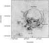 |
Fig. 1 Large scale DSS red image (north up, east left) of the star forming region NGC 6357. The main structures described in the text are marked and labelled. The white stars mark the positions of known star clusters. The length scale is drawn for an assumed distance of 1.7 kpc. |
This paper is organised as follows. In Sect. 2 we describe observations and data reduction. In Sect. 3, we present large-scale, deep Spitzer/IRAC photometry of NGC 6357, and briefly examine how YSOs are distributed in the region. In the same section, we then focus on Pismis 24 by using optical and infrared photometry, complemented with X-ray high-angular resolution observations from the literature. We carefully address many critical issues (such as crowding effects on the photometric completeness, contamination of cluster members by background stars, the reddening law, and infrared excess from young objects), some of which are especially important for studying regions lying in the Galactic plane and close in projection to the Galactic centre, but which have not been fully considered so far. We will also assess the limitations of the available YSO diagnostics, and their effects on data interpretation. The IMF of Pismis 24 is derived in Sect. 3.8. The stellar populations in the other clusters will be studied in forthcoming papers using recently obtained near-infrared (NIR) observations. A tentative scenario for star formation in the region is however discussed in Sect. 4. Finally, our conclusions are summarised in Sect. 5.
1.1. NGC 6357 and the open cluster Pismis 24
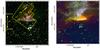 |
Fig. 2 Left. Three-colour image (J blue, H green, Ks red) of Pismis 24 and G353.2+0.9, obtained from the reduced SofI frames. Outlined, the HST/WFPC2 field. The border between the two sub-fields and the massive star N78 36 are also indicated. Right. For comparison, three-colour image of the same area obtained by combining the Spitzer/IRAC (short integration) frames at 3.6 μm (blue), 4.5 μm (green) and 8.0 μm (red). A colour version of this figure is available in the on-line edition. |
NGC 6357 is a complex composed of giant molecular clouds, Hii regions and open clusters, located at l ~ 353°, b ~ 1°, at a distance of 1.7 kpc (see Sect. 1.2). The large scale structure has been studied in a number of papers and its most prominent components are highlighted in Fig. 1. The gas distribution is outlined by a large optical shell opened to the north (named big shell by Cappa et al. 2011) and three smaller cavities (namely CWP2007 CS 59, CWP2007 CS 61, and CWP2007 CS 63; Churchwell et al. 2007). Lortet et al. (1984) noted that the big shell is in low-excitation conditions and ionisation-bounded, and suggested it is in fact a wind-driven bubble. Following Felli et al. (1990), we will refer to the big shell as the ring. Three Hii regions are associated with the cavities: G353.2+0.9 (inside CS 61), G353.1+0.6 (inside CS 63), and G353.2+0.7 (inside CS 59).
The big shell is ~60′ in diameter (~30 pc at 1.7 kpc) and is bordered by an outer shell of giant molecular clouds with LSR velocities in the range − 12.5 to 0 km s-1 (Cappa et al. 2011), The total estimated gas mass of the outer shell amounts to 1.4 × 10⁵M⊙. If the whole molecular gas structure is part of a large bubble, then the gas velocity range suggests an expansion rate of the order of ~10 km s-1. Given a radius of ~15 pc, the dynamical age of this large shell would be ~1.5 Myr.
CS 61 is situated inside the southern half of the big shell, enclosed in an elliptical ring of NIR emission (see Fig. 3) whose most prominent feature is the Hii region G353.2+0.9 in the northern part. A few molecular clouds border the NIR emission, with LSR velocities between − 7.5 and 0 km s-1 (Cappa et al. 2011), arranged in another shell structure (shell A, labelled in Fig. 1). The total estimated mass of shell A is 1.2 × 10⁵M⊙.
Pismis 24 (see Fig. 2) is a young open cluster inside CS 61, off-centred northward (as marked in Fig. 1). Several optical spectroscopic and photometric observations have unveiled a number of coeval (~1 Myr) O-type stars among its members (Moffat & Vogt 1973; Neckel 1978; Lortet et al. 1984; Massey et al. 2001; Russeil et al. 2012). The two brightest stars were identified as an O3 If (Pismis 24 1, a.k.a. HD 319718) and an O3 III (Pismis 24 17) star (Massey et al. 2001), respectively. Pismis 24 1 was then resolved by HST imaging into two components, Pismis 24 1SW and Pismis 24 1NE (the latter being a spectroscopic binary), of ≲100 M⊙ each (for a distance of ~2.56 kpc, larger than that assumed in the present work; Maíz Apellániz et al. 2007). We note that not necessarily these stars have already ended their main-sequence phase. Recent simulations of a non-rotating 60 M⊙ star have shown that this would display a supergiant appearance (i.e., luminosity class I) already on the zero age main sequence (ZAMS; Groh et al. 2014).
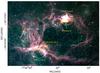 |
Fig. 3 Three-colour image (3.6 μm blue, 4.5 μm green, 8.0 μm red) of NGC 6357, obtained from the short-exposure IRAC frames. The large circles mark the locations of the most prominent Hii regions. The clusters Pismis 24 and AH03J1725–34.4 are also labelled. A colour version of this figure is available in the on-line edition. |
Wang et al. (2007) obtained deep X-ray Chandra/ACIS observations of Pismis 24, finding ~800 X-ray sources that cluster around Pismis 24 1 and Pismis 24 17, mostly intermediate- and low-mass PMS cluster members. The radial distribution of X-ray source surface density is characterised by a core ~2′ in radius superimposed on a halo with a radius of at least 8′. Optical (RI) photometry and spectroscopy (of a smaller sub-sample) with VIMOS at the VLT (Fang et al. 2012) confirmed that these are PMS stars with a median age of 1 Myr and an age spread in the range ≲0.1 to ≳10 Myr. In addition, the IMF is consistent with that of the Orion Nebula Cluster (ONC). Wang et al. (2007) estimated a number of members of ~10 000 if the distance is 2.56 kpc. By combining 2MASS and Spitzer/IRAC photometry, Fang et al. (2012) derived a very low fraction (~0.2) of stars with a circumstellar disk within ~0.6 pc from Pismis 24 1. This is quite low for such a young cluster, thus they suggested that this is observational evidence of the effect of massive stars on the disk evolution around nearby, less massive stars. The O-type stars in Pismis 24 are the ionising sources of G353.2+0.9 (Bohigas et al. 2004; Giannetti et al. 2012). They are also responsible for the ionisation of the inner edge of shell A, originating a ring of Hii regions collectively referred to as G353.12+0.86 by Cappa et al. (2011).
Spitzer/IRAC photometry showed three large clusters of Class I and Class II sources in NGC 6357 (Fang et al. 2012): one coinciding with Pismis 24, another coinciding with the open cluster AH03J1725-34.4 towards CS 63 (Dias et al. 2002; Gvaramadze et al. 2011), and a third one towards CS 59. The most massive members of AH03J1725–34.4 are N78 49, N78 50 and N78 51, that were classified as O5 to O9.5 (Neckel 1978; Lortet 1984), although Damke et al. (2006) recently reported a new spectral classification, namely O4III for N78 49 and O3.5V for N78 51, which suggests that AH03J1725–34.4 is roughly coeval with Pismis 24. N78 49 is the main ionising source of the Hii region G353.1+0.6 (Massi et al. 1997), located on the northern edge of CS 63, where a few giant molecular clouds lie between CS 63 and CS 61 (Massi et al. 1997; Cappa et al. 2011). Fang et al. (2012) also found two arcs of Class I and Class II sources, one encompassing CS 59 and CS 61, and the other in a symmetrically located position with respect to Pismis 24, which may be connected with the cluster.
A few authors have also suggested that an older population of stars may exist in NGC 6357. Wang et al. (2007), by noting the off-centred position of Pismis 24 inside CS 61, which might be inconsistent with a bubble originated by the energetic input from the stars of the cluster, and Gvaramadze et al. (2011), by noting the age discrepancy between the very massive members of Pismis 24 and the nearby (~4′ from Pismis 24) older WR93.
1.2. Distance to Pismis 24 and extinction
There is little doubt that the two most prominent Hii regions in NGC 6357, (namely. G353.2+0.9 and G353.1+0.6) are at the same distance. The gas velocity either from radio recombination lines or from mm molecular lines does not change appreciably from one to the other (Massi et al. 1997). In particular, large-scale 12CO(1–0) emission (Cappa et al. 2011) from the region displayed in Fig. 3 confirms the visual impression that we are merely observing parts of a larger complex. Remarkably, the nearby region NGC 6334 also exhibits similar gas velocities and stellar photometry yields a similar distance (Russeil et al. 2012). Therefore, NGC 6357 as a whole could be part of an even larger galactic complex.
The distance to NGC 6357, and to Pismis 24 in particular, is still debated. As explained in Massi et al. (1997), the kinematical distance (~1 kpc) based on the radial velocity of the associated gas is uncertain and it is now clear that it underestimates the actual distance. Neckel (1978) found 1.74 ± 0.31 kpc for NGC 6334 and NGC 6357 based on optical photometry of stars. Lortet et al. (1984) found the same value from spectroscopic observations of the most luminous stars in NGC 6357. Based on a spectral analysis of the most massive members of Pismis 24, Massey et al. (2001) found a distance of ~2.56 kpc (distance modulus DM = 12 mag), larger than the previous values. On the other hand, all the most recent determinations point to a distance ~1.7–1.8 kpc (Fang et al. 2012; Russeil et al. 2012; Gvaramadze et al. 2011; Lima et al. 2014). Reid et al. (2014) found an even lower distance to NGC 6334 (1.34 kpc) from trigonometric parallaxes of masers. In the present work, we will assume a distance 1.7 kpc (DM = 11.15 mag) following the most recent literature.
Part of the discrepancy in the distance determination may arise due to an anomalous reddening. Chini & Krügel (1983) had already noted that the region is seen through a dark cloud and derived RV = 3.7 ± 0.2. Bohigas et al. (2004) found RV = 3.5, which agrees with RV = 3.53 ± 0.08 obtained by Russeil et al. ([?]). However, Maíz Apellániz et al. (2007) found RV = 2.9 − 3.1 for the two most massive stars of Pismis 24 through HST optical and 2MASS NIR photometry.
Contrary to the distance, the average extinction towards Pismis 24 appears to be well constrained. Neckel (1978) and Lortet et al. (1984) found that the brightest members are affected by AV in the range 5–6 mag. Massey et al. (2001) found E(B − V) between 1.6–1.9 (i.e., the same AV range as above if RV = 3.1) and a median E(B − V) = 1.73 for the most massive stars. Maíz Apellániz et al. (2007) obtained AV = 5.5 mag for Pismis 24 1 and AV = 5.9 mag for Pismis 24 17, using HST optical photometry (values increasing to AV = 5.87 mag and AV = 6.34 mag, respectively, when including 2MASS photometry). Russeil et al. ([?]) found AV in the range 5.01–6.39 mag using multi-band photometry, and values in agreement with those of Maíz Apellániz et al. (2007) for the 2 most massive stars. Fang et al. (2012) used optical spectroscopy and RI photometry for a large number of low-mass counterparts of X-ray sources (hence, mostly cluster members) deriving an extinction range 3.2 <AV< 7.8. Lima et al. (2014) obtained an average E(J − Ks) = 1.01, i.e., E(B − V) = 1.75, for the cluster stars.
2. Observations and data reduction
2.1. Near-infrared imaging
The field towards G353.2+0.9 was imaged in the JHKs bands with SofI (Moorwood et al. 1998) at the ESO-NTT telescope (La Silla, Chile), during the night between 13 and 14 May, 1999. The plate scale is ~0.282′′/pixel, yielding an instantaneous field of view of ~5′ × 5′. For each band five pairs of on-source/off-source images were taken, dithered according to a pattern of positions randomly selected in a box of side length 20″. Each image consists of an average of 40 (80 at Ks) sub-exposures of 1.182 s, resulting in a total on-source integration time of ~4 min. (~8 min. at Ks). The raw images were crosstalk corrected, flat fielded (using dome-flats), sky subtracted, bad-pixel corrected, registered and mosaicked using the special procedures developed for SofI and standard routines in the IRAF1 package. The seeing in the final combined images is ~ . A three-colour image (J blue, H green, Ks red) from the reduced set of frames is shown in Fig. 2. The field covered is ~5′ × 5′ in size, approximately centred at RA(2000) = 17h24m45.4s, Dec(2000) = −34°11′25″. The Ks image was already used by Giannetti et al. (2012) in their Fig. 2, where the structures visible in the image are labelled. To calibrate the photometry, the standard star S279-F (Persson et al. 1998) was observed in the same night.
Photometry was carried out on the final images by using DAOPHOT routines in IRAF. We selected a ~1 (PSF-)FWHM aperture and sky annuli ~2 FWHM both in radius and width, with the modal value as a background estimator. From this, PSF-fit photometry was then performed with ALLSTAR. The results in the three bands were matched together by using a radius of 3 pixels (~1 FWHM). The obtained limiting magnitudes (at a signal to noise ratio of 3) are J ~ 19.7, H ~ 19 and Ks ~ 18.5. In total, we found 6500 NIR sources detected at least in the Ks band.
We compared our photometry with that from 2MASS, which is both less sensitive and less resolved than ours. By computing Δm = mag(SofI) − mag(2MASS) we found averages 0.05 ± 0.32 mag at Ks (0.03 ± 0.17 mag for Ks< 12), 0.09 ± 0.23 mag at H (0.05 ± 0.09 mag for H< 12), and 0.04 ± 0.30 mag at J (0.02 ± 0.09 mag for J< 12). The sources appear slightly fainter in the SofI photometry, as expected due to its better angular resolution. Such large dispersions in Δm are usually found in young, crowded stellar fields when comparing photometry of very different sensitivity and resolution. However, we note that Δm exhibits a similar spread as that of the 2MASS photometric uncertainties in the same band. Therefore, we can conclude that our SofI photometry is consistent with that from 2MASS within errors. We exploited this to add 9 2MASS sources (including Pismis 24 1, Pismis 24 17, and N78 36) to our photometry list, which are saturated in at least one of the SofI bands.
To estimate the completeness limits, we examined the histograms of number of sources as a function of magnitude. This was complemented with experiments of synthetic stars added to the images. To account for the different levels of extinction in the imaged field, this has been divided into two sub-fields: a northern one (encompassing the molecular gas region, thus more extincted) and a southern one (much less extincted, containing Pismis 24). For the sake of simplicity, the two sub-fields have been separated by a line of constant declination (Dec[2000] = −34°11′14″, see Fig. 2) bordering the southern edge of the structure named “bar” (see Fig. 2 of Giannetti et al. 2012). As expected, we found different completeness limits in the northern field, dominated by diffuse emission, and in the southern one, dominated by source crowding. We were able to retrieve ~80% of the artificial stars at Ks ~ 16.5 in the northern field, and at Ks ~ 15.8 in the southern field. We only carried out the test in the Ks band, However, we estimate that the completeness limits in the other bands can be obtained by adding the following value to the Ks completeness limit: 0.5 − 1 mag at H and 1 − 1.5 mag at J.
2.2. HST/WFPC2 optical data
We searched the HST archive for images of Pismis 24 suitable for photometry. We retrieved WFPC22 observations in the bands F547M and F814W from programme 9091 (P.I. Jeff Hester). These filters can be easily transformed to the Johnson-Cousins VI standard. Pismis 24 was observed on April 11, 2002. The images we used had an integration time of 500 s. To check the transformations to the VI standard, we also searched for WFPC2 images of clusters through the same bands with in addition VI photometry from the ground in the literature. We found observations of the open cluster NGC 6611 from the same programme (9091) meeting this requirement, carried out on August 8, 2002. As known, the WFPC2 field of view is covered by four cameras, each of which 800 × 800 pixels in size. Three of them (WFC) are arranged in an L-shaped field and operate at a pixel scale of ~ , the fourth one (PC) operates at a pixel scale of ~
 .
.
Removal of cosmic rays and photometry was performed using HSTphot v1.1 (Dolphin 2000), a software package specifically developed for HST/WFPC2 images. Quite a few stars in the two fields (i.e., Pismis 24 and NGC 6611) were rejected because saturated. HSTphot transformed the photometry to the Johnson-Cousins standard by using the relations provided by Holtzman et al. (1995). Thus, stars without simultaneous detections in both bands were also discarded. Since the detection limit is V ~ 25, and V − I> 4 for most of the stars, these generally have I< 21. In total, we obtained VI photometry for 158 stars in Pismis 24 and 397 stars in NGC 6611, from all four chip fields (PC and WF). The HST/WFPC2 field of view is outlined in Fig. 2. Almost all the stars have photometric errors <0.05 in I and <0.1 mag in V, although a few stars with V> 24 have photometric errors in V up to ~0.2 mag.
We compared our results with the ground-based photometry in the same bands. Unfortunately, no ground-based photometry is available for Pismis 24 in the V band, although we were able to use that from Fang et al. (2012), obtained from VIMOS observations, in the I band. However, ground-based photometry in the VI bands is available for NGC 6611, obtained from WFI (at the 2.2 m telescope of ESO) observations (Guarcello et al. 2007). Thus, we discovered an offset (0.28 ± 0.38 mag) between our V photometry of NGC 6611 and that from Guarcello et al. (2007), with no apparent colour effects. Nevertheless, a clear colour effect was found on our I photometry of both clusters (after correction, the r.m.s. of the difference in I magnitudes is ~0.25 mag). This is hardly surprising: Holtzman et al. (1995) caution about their transformations being accurate only in the range − 0.2 <V − I< 1.2, whereas most of the sources towards Pismis 24 are well above V − I = 1. Thus, we derived a more accurate transformation for I through a linear fit. Then, we corrected our VI photometry to match the corresponding ground-based photometry.
2.3. Spitzer/IRAC data
The InfraRed Camera (IRAC, Fazio et al. 2004) on board the Spitzer Space Telescope, is equipped with four detectors operating at 3.6, 4.5, 5.8 and 8.0μm, respectively. Each detector is composed of 256 × 256 pixels with a mean pixel scale of  , yielding a field of view of
  . We retrieved all Spitzer/IRAC observations towards NGC 6357 from the Spitzer archive. After a close examination of the available data, we decided to use those from Program ID 20726 (P.I. Jeff Hester). The IRAC observations were carried out in 2006, September 28, during the cryogenic mission. The high dynamic range (HDR) mode was used, meaning that two images per pointing were taken, a short exposure one (0.4 s) and a long exposure one (10.4 s). This allows one to obtain unsaturated photometry of bright sources from the short-exposure image and deeper photometry of faint sources from the long-exposure one.
Data reduction is detailed in Appendix A and yielded two mosaicked images (short- and long-exposure) per band, with a pixel size  (about half the native pixel size). We cropped each of them to a final field of view of ~38′ × 26′ encompassing shell A and the three clusters in NGC 6357, fully covered at all bands. A three-colour (3.6 μm blue, 4.5 μm green, 8.0 μm red) image of the field, obtained from the final short-exposure IRAC frames, is shown in Fig. 3.
We performed aperture photometry on the final IRAC mosaics (both long- and short-exposure) by using DAOPHOT routines in IRAF. We adopted an aperture radius of 4 pixels and a sky annulus 4 through 12 pixels from the aperture centre (i.e., 2 and 2–6 native pixels, respectively), with the median value as a background estimator. These radii were chosen as small as possible to account for the variable diffuse emission in many areas of the region. We used the corresponding aperture corrections given in Table 4.7 of the IRAC instrument handbook (version 2.0.1). Short-exposure and long-exposure photometry were matched in each band, adding the brightest sources from the former to the faintest sources from the latter. The photometry is further detailed in Appendix B, where we also show that GLIMPSE II photometry and ours are consistent with each other, and that the detection limits are similar, although GLIMPSE II photometry is much less deep and should consequently be less sensitive. We attribute this to source crowding causing our photometry to be confusion-limited (NGC 6357 is in the Galactic plane, few degrees from the Galactic centre).
After combining long- and short-exposure photometry, there remained 65 875 sources in the 3.6 μm band, 59 160 in the 4.5 μm band, 47 398 in the 5.8 μm band, and 13 763 in the 8.0 μm band. We further merged the 4 lists of objects by adopting a matching radius of 3 pixels ( ). This is about equal to the FWHM of the Spitzer PSF (Fazio et al. 2004) at those wavelengths.
Contamination due to PAH emission (and its cleaning) is discussed in Appendix B. To reduce any remaining effects from artefacts or false detections, in the following we will only consider sources detected in at least the first two bands (i.e., 3.6 and 4.5 μm), and with photometric errors <0.3 mag. In addition, we will always discard detections with photometric errors ≥0.3 mag when adding other bands, unless otherwise stated. This means that multiple-band detections will be discarded if the photometric error is ≥0.3 in any of the bands. Nevertheless, we show in Appendix C that the effect on source statistics is negligible.
The photometric completeness limit is highly variable, decreasing in magnitude according to the number of bands where simultaneous detection is required, and depending on the position in the image. In addition, the long exposure images are mostly saturated over the areas of intense diffuse emission, particularly in the two upper wavelength IRAC bands (i.e., 5.8 and 8.0 μm), and only the short exposure ones were suitable for photometry there. The completeness limits are derived in Appendix C and listed in Table C.1. In summary, we found that sources detected in at least the first two bands should be almost complete down to [3.6] = [4.5] = 12.25 in areas with at most faint diffuse emission, and [3.6] = [4.5] = 10.75 in areas with intense diffuse emission.
2.4. Matching of optical, NIR, MIR, and X-ray detections
We complemented the optical, NIR, and mid-infrared (MIR) observations with Chandra/ACIS-I X-ray observations from Wang et al. (2007). These cover a field of view of 17′ × 17′ centred at RA(2000) = 17h24m42s, Dec(2000) = −34°12′30″, with sub-arcsec angular resolution at the centre. Since we only use the detections in the area covered by SofI, which lies at the centre of the ACIS field of view, no significant degradation of the X-ray PSF is expected. The total integration time is ~38 ks.
Estimated [3.6] completeness limits and corresponding stellar masses for given extinction values.
First, we merged our NIR source list with that from the X-ray observations by using IRAF routines and a matching radius of ~1 arcsec. The optical, NIR-X and IRAC databases were then merged again with the same matching radius. We constructed a larger catalogue (without optical data) with the sources falling in the whole SofI field (see Table 1), and a smaller one with all the sources falling in the HST/WFPC2 field (see Table 2).
Out of the 665 X-ray sources and 114 X-ray tentative sources found by Wang et al. (2007), 337 sources and 52 tentative sources fall in our SofI field. Of these, 303 sources and 33 tentative sources match a detection in at least the Ks band. As for the unmatched X-ray sources, 15 (plus 2 tentative) fall towards either of the two most massive cluster members, where some SofI sources are saturated and others may well be hidden inside the high-count wings of the O stars.
Out of the 6500 Ks sources in our larger catalogue, 3308 were also detected at J and H, 2322 only at H, and 1660 match a source of the IRAC catalogue. Only 88 IRAC sources do not have a match with a NIR source in the Sofi field. The smaller catalogue (HST field) contains 1140 NIR sources with at least a detection in the Ks band, 36 sources only detected in the X-ray, and 11 sources only detected in VI. The optical sources with a NIR counterpart are 147 (for conciseness, by NIR counterpart we will mean a source at least detected in the Ks band). Of these, 62 have also been detected in the X-ray. Finally, 29 X-ray sources have infrared counterparts but not an optical one. In the following sections we will always discard NIR detections with photometric errors >0.3 mag in any of the bands, as done for IRAC data, unless otherwise stated.
3. Results
3.1. IRAC selection of young stellar objects
Robust criteria to identify YSOs have become available in the literature based on IRAC colours. We first removed contaminants from our catalogue of IRAC sources by following Gutermuth et al. (2009). As shown in Appendix D, the major source of contamination is PAH emission at 5.8 and 8.0 μm, which can be associated with faint 3.6 and 4.5 μm sources located in areas with strong diffuse emission. We removed these PAH contaminants from the list of all IRAC sources detected in at least the first three IRAC bands.
Then, we used the criteria of Gutermuth et al. (2009) to also remove PAH galaxies, broad-line AGNs, and unresolved knots of shock emission from the sources detected in all 4 bands. Since only shock emission can be identified based on the first three bands, (all other contaminants also requiring a measurement at 8.0 μm), extragalactic sources could not be filtered out of the sample of objects only detected in the first three bands. However, extragalactic contaminants are probably less of a problem since we are observing through the galactic plane. The very high reddening behind NGC 6357 should efficiently extinct most of the background galaxies to below our detection limits.
More critical contamination may arise due to evolved background stars (i.e., AGB stars) whose infrared colours can mimic those of YSOs (Robitaille et al. 2008). But these, unlike YSOs, should exhibit a more homogeneous spatial distribution inside our field like any other type of background stars, although still patchy due to extinction variations.
Finally, after contaminant cleaning we identified the Class I and Class II sources following the colour criteria of Gutermuth et al. (2009). We show in Appendix C and Sect. 3.2 (see also Table 3) that only the brightest and most massive Class II sources can be simultaneously detected in all IRAC bands, particularly in the areas with intense diffuse emission. The sample can be enlarged to include less massive young stars by requiring detections in the first three IRAC bands only, but the stellar mass corresponding to the completeness limit still remains quite high towards the areas of intense diffuse emission. Altogether, we found 50 Class I sources and 482 Class II sources out of 4560 sources with detections in all bands, and a further 14 Class I sources and 729 Class II sources out of 9114 sources with detections in the three lower-wavelength bands only. Their colours are shown in Fig. D.4. The number of YSOs classified from their colours in all four bands can be compared with those found by Fang et al. (2012) in a similar area, who used IRAC photometry in all four bands with a sensitivity comparable to that of our photometry. They retrieved 64 Class I/flat sources and 244 Class II sources. While the numbers of Class I sources found are consistent, we found twice as many Class II sources as they did. This is not only due to the different colour classification criteria adopted: by their criteria (and using their cuts in photometric errors as well), we still found 438 YSOs. It is likely that the much longer integration of our images yields more accurate measurements of faint objects allowing more sources to get through the photometric error cuts.
3.2. Spatial (large-scale) distribution of IRAC sources
The completeness limits listed in Table C.1 can be converted into mass completeness limits if distance, mean age and average extinction of the stellar population are known. We will assume that Pismis 24 is roughly representative of the stellar populations in most of the clusters of NGC 6357, which is confirmed by the results of Getman et al. (2014) and Lima et al. (2014). Thus, we adopt a distance modulus of 11.15 mag, and an extinction AV ~ 5.5 mag (see Sect. 1.2). Using the reddening laws of Rieke & Lebofski (1985) and Indebetouw et al. (2005), this translates into A3.6 ~ 0.34, mag and A4.5 ~ 0.26 mag. We also assume that the IRAC 3.6 μm band measurements are consistent with L-band measurements, so that stellar masses can be derived from theoretical L values. The latter were obtained by using the PMS evolutionary tracks (1 Myr old) of Palla & Stahler (1999) and Siess et al. (2000), complemented with the colours of Kenyon & Hartman (1995). In the evolutionary models of Palla & Stahler (1999), their birthline coincides with the ZAMS for stars ≳8–10 M⊙, so we also used the colours of Koornneef (1983), and the spectral types from Habets & Heinze (1981) to convert the brightest [3.6] values into masses. The estimated mass completeness limits are listed in Table 3.
Towards areas with intense diffuse emission (e.g., G353.2+0.9 north of Pismis 24), coinciding with local molecular clouds, both the reduced sensitivity and the higher extinction must also be taken into account. Table 3 lists mass completeness limits, as well, for AV = 10 − 20 mag. Clearly, these areas may suffer from heavy incompleteness.
Due to their infrared excess, the mass completeness limit is bound to be lower for Class II sources. One can obtain very crude estimates of this as follows. First, we assume a spectral index dlog λFλ/ dlog λ = −1 (representative of Class II sources). Then, we derive the flux in the J band from the completeness [3.6] value and the spectral index. Since the flux in the J band is less affected by the excess, we use the J-band magnitudes obtained and the same evolutionary tracks as above to derive the corresponding stellar masses. The values yielded are listed in Table 3, as well. For Class I sources, estimates are much more difficult to make. As an example, the model in Whitney et al. (2003) of a Class I source with a 0.5M⊙ central star is always fainter than our faintest completeness limit (i.e., [3.6] = 12.25), whereas the one in Whitney et al. (2004) with M∗ = 0.5 M⊙ and T∗ = 4000 K would be brighter unless it is seen with the disk edge-on.
To map the surface density of young stars in the whole NGC 6357 region, we counted the IRAC sources in squares 1′ in size, displaced by  from each other both in right ascension and in declination (i.e., a Nyquist sampling interval). We included all sources with simultaneous detection in at least the 3.6 and 4.5 μm bands up to [3.6] = 12.25. As shown in Table 3, this limit should allow us to retrieve most of the young stars down to 2–3 M⊙ outside the areas of the image with intense diffuse emission (e.g., away from G353.2+0.9 and G353.1+0.6). We also tried a 2D binned kernel density estimate as done in Sect. 3.3, which gave similar results although yielding a slightly smoother distribution. In this case, the routine dpik returns 33″ − 46″ as optimal bandwidths, which justifies our choice of a 1′ sampling size.
The area imaged is large enough to enable us to derive a meaningful average for the source surface density of background stars. The count statistics is shown as a histogram in Fig. 4, obtained by sorting all 1′ size squares. It resembles a Poisson statistics but exhibits an excess frequency towards high counts, produced by non-random clustering. The peak is roughly fitted by a Poisson curve with mean equal to 14 stars/arcmin2, also shown in Fig. 4, that we assume to be the mean surface density of field stars (~14 ± 4 stars/arcmin2).
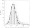 |
Fig. 4 Histogram of the statistics of the surface distribution of IRAC sources detected at least in the two lower-wavelength bands, counted in squares 1′ in size, displaced each other by |
The surface density distribution of IRAC sources obtained is shown in Fig. 5. The lowest contour is equal to the mean field star density (14 stars/arcmin2) plus a 3σ of the fitted Poisson distribution (11 stars/arcmin2), and the contour step is 3σ. The three larger clusters (Pismis 24, AH03J1725–34.4, hereafter A, and the one roughly located towards G353.2+0.7, hereafter B) stand out well above a 3σ fluctuation of the field star statistics. They are associated with the three cavities identified by Churchwell et al (2007; see Sect. 1.1 for details), close in projection to high density gas clumps where Hii regions (G353.2+0.9, G353.1+0.6, and G353.2+0.7) are produced by ionisation from their massive members. Thus, the three clusters are situated towards the brightest parts of (or outside) the ring-like structure (i.e., in the north and east) surrounding CS 61, as evident in Fig. 3
Each cluster appears further subdivided in several subclusters at the 1′ resolution scale. We provide a tentative list of their properties in Table 4, including approximate positions based on those of the local peaks of surface density. Number of sources and size are computed with respect to the 3σ level above the average field star surface density.
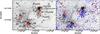 |
Fig. 5 Left. Contour map of the surface density of IRAC sources, computed as explained in the text. Only sources detected in at least the first two Spitzer/IRAC bands, with photometric errors <0.3 mag, and up to [3.6] = 12.25 are considered. The contours are: 25 stars/arcmin2, 36 stars/arcmin2 (red line), 47 stars/arcmin2, ranging in steps of 3σ (11 stars/arcmin2) from the estimated average surface density (14 stars/arcmin2) of field stars plus 3σ, overlaid on the image at 3.6 μm (grey-scale). Also labelled, the tentatively identified subclusters (A is also known as AH03J1725–34.4). Right. Same as left, but with the positions of identified Class II sources (full blue squares) and Class I sources (open red triangles) superimposed. Other YSO concentrations are enclosed in dashed-line circles. A colour version of this figure is available in the on-line edition. |
We named “cores” the maxima of surface density towards the three clusters. As shown in Fig. 5 and Table 4, both Pismis 24 and AH03J1725-34.4 stretch to the edge of the bright diffuse emission areas (where most of the molecular gas is also located). Checking the effects of contamination, we found that by removing from the counts all sources with detections in 3 and 4 bands identified as contaminants, lower surface densities are obtained towards the areas with diffuse emission. Consequently, none of the contours in the modified map cross these regions, and subclusters Pis24 E, Pis24 N, BS, and AW almost disappear. Both contamination and decreased sensitivity make it difficult to identify clustering towards these bright areas. However, the remaining subclusters can still be retrieved in the modified map suggesting they are real local structures. This is further confirmed by the distribution of the YSOs, i.e., all Class I and Class II sources identified using at least the first three IRAC bands (shown in Fig. 5, as well). In fact, Kuhn et al. (2014), using the MYStIX database, essentially retrieved our subclusters Pis24 core (their NGC 6357 A), Pis24 S (NGC 6357 B), Acore (NGC 6357 C), AS (NGC 6357 D), and AE (NGC 6357 E). In addition, Lima et al. (2014), using VVV NIR photometry, also noted our subcluster Pis24 W (VVV CL164), but suggested that it is a much older cluster (~5 Gyr) unrelated with NGC 6357. Out of the clusters studied by Lima et al. (2014), our Acore and AS roughly coincide with their BSD 101 and ESO 392-SC 11, respectively.
Main parameters of the clusters of IRAC sources.
Clearly, the YSOs concentrate towards the three clusters. An underlying diffuse population of Class II sources is also visible, although this could be contaminated by background evolved stars displaying the same colours. The arc-like distributions of YSOs claimed by Fang et al. (2012), symmetrical to the centre of the largest bubble, show up south-east of Pismis 24 (roughly overlapping both our cluster A and our cluster B) and north-west of it (four circled areas in Fig. 5). The Class I sources appear to avoid the largest peaks of IRAC source surface density in the area; rather they tend to be found towards the molecular clouds (compare with Fig. 5); for example, east of Pis24 core, north of Acore, and north of BN. The four encircled areas showing small YSO concentrations also lie towards molecular gas clumps. Only few Class I and Class II sources are found towards the Hii regions G353.2+0.9 and G353.1+0.6, but this is probably due to the incompleteness. We can therefore conclude that star formation appears to be in progress in the molecular gas associated with the clusters.
3.3. NIR stellar population of Pismis 24 and reddening law
The members of Pismis 24 can be clearly isolated in the NIR colour–colour diagrams (CCD) shown in Figs. 6a,b of the sources found with SofI. Only sources with Ks< 16 (roughly the completeness limit in the southern field, as discussed in Sect. 2.1) have been selected. We have overplotted both the main sequence locus (thick solid lines, Koornneef 1983) and the reddening band of the main sequence (dashed lines) according to the extinction law derived by Rieke & Lebofsky (1985). The latter usually fits well the reddening of NIR sources whose photometry is obtained in the SofI filters (e.g., Massi et al. 2006).
A smoothing of the datapoints (contours in Fig. 6) unveils two different stellar populations in the CCD. To this purpose, we computed a 2D binned kernel density estimate using the routine bkde2D from the library KernSmooth in the package R (R core team 2014). The bandwidth was estimated using the routine dpik, which is based on a direct plug-in methodology (see Wand & Jones 1995). Two different datapoint concentrations can be distinguished along the main sequence reddening band, roughly separated by H − Ks = 1 and J − H = 2. The less reddened concentration is roughly centred at AV ~ 5 mag from the main sequence and extends up to AV ~ 10–15 mag, i.e., it lies in the reddening interval of the cluster (see Sect. 1.2). The two features are easily recognised in the magnitude–colour diagrams (Ks vs. H − Ks, hereafter CMD) of Figs. 6c,d. The smoothed distribution using a 2D binned kernel density estimate is also shown. Here, the less reddened concentration appears as a branch extending from the massive stars Pismis 24 1 and Pismis 24 17 down to the completeness limit, displaying a larger colour spread in the northern field.
The two concentrations are clearly separated in the CCD by a sort of gap, which is more evident in the northern field. This suggests that the gap is caused by the molecular gas associated with NGC 6357 and allows one to discriminate between background stars (the more reddened concentration) and a nearby population of mostly cluster members (the less reddened concentration). The foreground extinction can be easily estimated from the distance between the ZAMS and the outer envelope of sources facing the ZAMS in Fig. 6d, ranging from AV ~ 5.7 mag to AV ~ 7.6 mag. This is consistent with the average reddening measured for Pismis 24 (e.g., Massey et al. 2001; Fang et al. 2012).
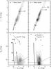 |
Fig. 6 a) SofI J − H vs. H − Ks diagram for the northern field. b) SofI J − H vs. H − Ks diagram for the southern field. c) SofI Ks vs. H − Ks diagram for the northern field. d) SofI Ks vs. H − Ks diagram for the southern field. Only sources with Ks< 16 and photometric errors <0.3 mag have been selected for the colour–colour diagrams, whereas all sources with photometric errors <0.3 mag in H and Ks have been selected for the colour-magnitude diagrams. The datapoint density after smoothing is shown with contours in all panels. The grey triangles mark the sources whose colours have been taken from 2MASS. A few of these sources, associated with Pismis 24, are also indicated, although those labelled G1, G2, and G3 are the candidate background giant stars discussed in the text. The main sequence locus is drawn in all panels with a thick solid line (using the colours from Koornneef 1983, complemented with the absolute magnitudes from Allen 1976 for panels c), d)). Spectral types are labelled next to the ZAMS in panel c). The dashed lines in panels a), b) are reddening paths with crosses every AV = 10 mag (from AV = 0 mag), according to Rieke & Lebofsky (1985), while the thin solid lines are the reddening paths according to the extinction law derived by Straiz˘ys & Laugalys (2008). The dashed line in panels c), d) marks the completeness limit. The arrow in panel c) spans a reddening of AV = 20 mag. Also shown as a full line parallel to the ZAMS in panel c) is the sequence of PMS stars 1 Myr old from the evolutionary tracks of Palla & Stahler (1999), for AV = 10 mag, and masses in the 0.1–6 M⊙ range. A distance of 1.7 kpc is assumed for ZAMS and isochrones. |
Interestingly, the more reddened datapoint concentration extends above the extincted main sequence band in the CCD. This is also evident using less deep 2MASS photometry and the extinction law of Indebetouw et al. (2005), which is based on large-scale 2MASS photometry. A possible explanation is that the extinction law in the area has a higher E(H − Ks) /E(J − H) ratio than 1.72, derived by Rieke & Lebofsky (1985). In fact, as shown in Figs. 6a,b (thin solid lines), the steeper law found by Straiz˘ys & Laugalys (2008), with E(H − Ks) /E(J − H) = 2, would make the main sequence reddening band encompass the more reddened source concentration. This would also imply a larger fraction of sources with a NIR excess (YSOs) associated with the cluster. Given the many claims of an anomalous RV in the region (see Sect. 1.2), we have also tried the extinction laws tabulated in Fitzpatrick (1999) as a function of RV. However, our conclusion is that there is no need for an extinction law significantly steeper than that of Rieke & Lebofsky (1985), which we conservatively adopt in this work. The shift of the redder clump is mostly due to a predominance of background giant and supergiant stars, whose locus lies slightly above that of the main sequence in the CCD, whereas main sequence stars become too faint to be detected and this somewhat depopulates the main sequence reddening band (e.g., a G0 V star would be fainter than Ks = 16 for AV = 15 mag even at the distance of Pismis 24). This is confirmed by three stars which are bright enough to be saturated, despite being very reddened (AV ~ 20 mag). They are labelled in Fig. 6 as G1, G2, and G3, among the sources whose NIR magnitudes have been taken from 2MASS. We checked that they lie far from the brightest stars of Pismis 24, two of them being at opposite sides in the images. Their reddening identifies them as background stars, and their intense brightness points towards them being giant or supergiant stars. As such, their correct location in the CCD is above the extincted main sequence band, which is more consistent with the extinction law by Rieke & Lebofsky (1985).
Figures 6c,d also show how deep our observations are. The completeness limit Ks = 16 can be converted into a mass limit by using the adopted distance modulus 11.15 mag and assuming a PMS stellar population 1 Myr old. From the evolutionary tracks of Palla & Stahler (1999), the corresponding mass completeness limit is 0.2 M⊙ for AV = 10 mag (appropriate for Pismis 24). We showed in Sect. 2.1 that the completeness limit in the northern field is Ks = 16.5; by adopting this value we find masses of 0.4M⊙ for AV = 20 mag (appropriate for young stars embedded in the molecular clouds). In a scenario of sequential star formation, one may expect a population of younger stars in the molecular gas than the (triggering) cluster members, hence intrinsically brighter and less massive at the completeness limit. On the other hand, if the region were farther away then the mass at the completeness limit would be accordingly larger (e.g., at ~2.56 kpc, Ks = 16 and AV = 10 mag would correspond to a ~0.4 M⊙ star).
3.4. X-ray source population of Pismis 24
It has long been known that X-ray surveys are very efficient in revealing populations of weak-line T Tauri stars (or Class III sources), given that these PMS stars are much brighter in X-rays than their main sequence counterparts (see e.g., Feigelson & Montmerle 1999). Classical T Tauri stars (or Class II sources) are also strong X-ray emitters, but these can be efficiently recognised based on their infrared excess, as well. So, the distribution of X-ray sources in star forming regions usually reflects that of PMS stars with and without a prominent circumstellar disk.
The high spatial resolution X-ray survey of NGC 6357 by Wang et al. (2007) provides a clear view of how Class II/III sources are distributed inside Pismis 24. The JHKs colours of the NIR counterparts of the X-ray sources (see Sect. 2.4) can be used to check their nature as PMS stars. The J − H vs. H − Ks diagram in Fig. 7 confirms this and is consistent with Fig. 6 of Wang et al. (2007), although we retrieve many more NIR counterparts from our deeper SofI photometry. In particular, 278 (out of 303) Ks counterparts (plus 25 out of 33 Ks counterparts of tentative X-ray sources) were also detected in the J and H bands with photometric errors <0.3 mag. Most datapoints populate the reddened main sequence region (which occurs for Class III source, as well), between AV ~ 5 and 10 mag, and some extend below it, exhibiting a NIR excess. This is consistent with a population of PMS stars. We note that the reddening law of Rieke & Lebofsky (1985) fully accounts for the colours of this population, further supporting its adoption (Sect. 3.3).
To estimate the fraction of X-ray emitting sources with a NIR excess, we counted all datapoints more than 1σ (where σ is the photometric error of each source) below the line defined by the reddening path from a main sequence M8 star (according to the colours from Koornneef 1983). Such MS stars (at the distance of the cluster) are too faint to be detected in our SofI image, so most of the objects below this line must be young stars with a colour excess. Out of the 303 X-ray emitting sources with detections in JHKs, 47 (~15%) exhibit a colour excess and can be classified as Class II sources. However, we will show in Sect. 3.7 that the fraction of NIR counterparts with a colour excess is actually higher than that derived from the colour–colour diagram of Fig. 7. Wang et al. (2007) estimate that the contamination from extragalactic sources is less than 2–4% and that from foreground stars less than 1–2%. We can therefore confirm that the X-ray sources from Wang et al. (2007) falling in our SofI field mostly represent a population of Class II/Class III sources belonging to the cluster.
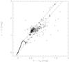 |
Fig. 7 SofI J − H vs. H − Ks diagram for the NIR counterparts of the X-ray sources detected towards Pismis 24. Only sources with photometric errors <0.3 mag have been selected. The thick solid line is the main sequence locus (using the colours from Koornneef 1983). The dotted lines are reddening paths with crosses every AV = 10 mag, following Rieke & Lebofsky (1985). |
The sensitivity of the X-ray observations can also be estimated following Wang et al. (2007). They quote an on-axis detection limit of 3 counts (0.5 − 8 keV) and derived a corresponding absorption corrected luminosity in the 0.5 − 8 keV band log (LX/ [erg s-1] ) ~ 30.2 at d = 2.56 kpc, which scales to log (LX/ [erg s-1] ) ~ 29.9 at 1.7 kpc. These can be converted into stellar masses using the empirical relationship found by Preibisch & Zinnecker (2002) for a ~1 Myr old PMS star population, obtaining M ~ 0.7 M⊙ (at 1.7 kpc). We note that from the best fit of Flaccomio et al. (2012) to CTTSs we obtained similar results. This is what one can expect in the southern field. To assess the effects of reddening in the northern field, we repeated their calculations using PIMMS3, but assuming an extinction AV = 20 mag. In this case, we obtained log (LX/ [erg s-1] ) ~ 30.6 and M ~ 1.8 M⊙ (d = 1.7 kpc).
The completeness of the NIR counterparts of the X-ray sources has been estimated in Appendix E to be at Ks ~ 13in the southern field. Assuming a distance of 1.7 kpc and adopting the evolutionary tracks of Palla & Stahler (1999) for 1 Myr old PMS stars, this corresponds to a mass completeness limit of ~2 M⊙ for AV between 5–10 mag, which is consistent with what was found by Wang et al. (2007).
3.5. Spatial distribution of young stars and YSOs towards Pismis 24
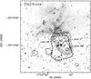 |
Fig. 8 Contour map of the surface density of NIR sources from the SofI data, overlaid with the Ks image of Pismis 24 and G353.2+0.9. Contours range from 240 stars arcmin-2 (the average for field stars plus 2σ, using the values found in the southern field) in steps of 30 stars arcmin-2 (~1σ). Also overlaid: (dashed contour) the surface density of IRAC sources (level 36 stars arcmin-2 of Fig. 5) delineating Pis24 core; (open circles) the location of sources with a NIR excess (see the text for the selection criteria). All data used in figure have Ks< 16 and photometric errors <0.3 mag both in Ks (surface density) and in all JHKs bands (NIR excess). |
Main parameters of the core of Pismis 24 (Pis24 core).
To derive the surface density of NIR sources from the SofI data towards Pismis 24 and G353.2+0.9, we followed the same method as in Sect. 3.2. We used squares of side ~29″ (100 pixels), i.e., half the size of the squares used for the IRAC sources, and counted sources up to Ks = 16 over the whole Ks image. To estimate the average surface density of field stars, we constructed the histograms of number of squares as a function of counts per square separately for the northern and the southern fields. In both cases, we obtained quasi-Poissonian distributions with an excess frequency of high counts. There is actually a slightly higher frequency of lower counts, as well, particularly in the northern field, which is probably caused by varying extinction. The average field star surface density was estimated from the peaks of the distributions and is ~180 stars arcmin-2 in the southern field, and ~80 stars arcmin-2 in the northern one. The standard deviation in the southern field is ~30 stars arcmin-2. In Fig. 8, a contour map of the surface density of NIR sources is overlaid on the Ks image, starting from 240 stars arcmin-2 (i.e., the average of field stars plus 2σ, using the values found in the southern field). Clearly, we retrieve the Pis24 core found from the IRAC data and discussed in Sect. 3.2, although it appears slightly smaller in Ks. This is not unexpected, given that the IRAC field is much larger and hence allows a better determination of the average surface density of field stars. Conversely, even the outer parts of the SofI field do probably include cluster members and all bins are therefore biased. However, this will mostly affect the statistics of cluster members rather than the peak locations. Heavy reddening could distort the surface density of NIR sources, as well. This may well occur north of the bar (i.e., in the northern field) where most of the associated molecular gas is distributed (Massi et al. 1997; Giannetti et al. 2012), but the southern field is expected to be much less affected and the most prominent surface density peaks are expected to outline real structures there.
The core of Pismis 24 appears elongated in a NE-SW direction, with three smaller subclusters: a central one (core C) including the massive stars Pismis 24 1 and Pismis 24 17 (although they are a bit off-centre, there is a local peak of density towards Pismis 24 1, not shown in the figure), a small compact concentration of stars between core C and the elephant trunk (core NE), and the highest peak of surface density, which lies in the south-west (core SW). Lima et al. (2014) suggest that core NE (their VVV CL 164) is a subcluster of Pismis 24, as well. They also indicate a further subcluster (their VVV CL 166), roughly located towards one of the regions in our image with counts 2σ above the average field star density.
The sources with a NIR excess are marked by small circles in Fig. 8. These have been selected as all sources with Ks< 16 lying in the colour–colour diagram on the right of the reddening line passing through the colours of main sequence late M stars (roughly coincident with the lower of the pair of lines drawn in Figs. 6a,b as dashed lines). These NIR-excess objects are distributed all over the field, but their number decreases in the northern field and they tend to concentrate towards both the Pis24 core and the Hii region. Background AGB stars can mimic the colours of YSOs and may then contaminate the field (Robitaille et al. 2008), but they are not expected to exhibit strong clustering, although they would as well tend to avoid the heavily extincted areas. Most of the sources with a NIR excess then represent real YSOs.
We estimated the number of cluster members in the core by counting the sources (up to Ks = 16) within the contour corresponding to 240 stars arcmin-2. We subdivided this area in three parts roughly coinciding with the subclusters. The results are listed in Table 5. The average density of field stars has been subtracted and the errors given are obtained by just propagating the Poissonian ones. The total number of members is larger than that found by counting IRAC sources (see Table 4). Although this is obvious, due to the differences in the mass completeness limits and resolutions between the two datasets, we would have expected to retrieve much more core members from the Ks image. This will be discussed in Sect. 4.2.
More specifically, various samples of different indicators can be used to derive the spatial distribution of YSOs in Pismis 24. In fact, given the nature of the region and the many connected effects already discussed, and the different completeness limits in the various bands, different indicators trace different types of sources with inhomogeneous results. For example, as discussed in Sect. 3.4, X-ray sources trace T Tauri stars, whereas in principle, we can use the IRAC colours to discriminate Class I and Class II sources following Gutermuth et al. (2009).
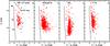 |
Fig. 9 Ks vs. H − Ks for the NIR counterparts of the YSOs towards Pismis 24 identified according to four different indicators, as explained in the text. Open symbols always refer to sources in the northern field, whereas full symbols refer to sources in the southern field. a) YSOs identified on the basis of their IRAC colours (triangles: Class I; squares: Class II); b) YSOs identified on the basis of their combined JH(HKs) [4.5] colours; c) YSOs identified on the basis of their JHKs colours; d) NIR counterparts of X-ray sources. The thick solid vertical line marks the main sequence locus (using absolute magnitudes from Allen 1976 and colours from Koornneef 1983) for a distance modulus of 11.15 mag (d = 1.7 kpc). The arrow in a) shows a reddening of AV = 20 mag according to Rieke & Lebofsky (1985). Spectral types are labelled on the ZAMS. A colour version of this figure is available in the on-line edition. |
NIR photometry can be used to identify stars with colour excess typical of circumstellar disks. For this purpose we used the criterion discussed in Sect. 3.4, based on the J − H vs. H − Ks diagram. Our SofI photometry is much deeper than the IRAC one, but it has been known that stars with circumstellar disks may not exhibit a colour excess in JHKs CCDs (Haisch et al. 2001) and a fraction of YSOs is likely to be missed. To make the most out of NIR and IRAC photometry, we combined the NIR fluxes with that in the IRAC 4.5 μm band. The first two IRAC bands are the most sensitive of the four and are much less affected by problems of saturation than the two longer wavelength bands. We adopted the criteria of Winston et al. (2007) to identify YSOs by using J − H vs. H − [4.5] or, when J is not available, H − Ks vs. Ks − [4.5] diagrams (not shown). These will be referred to as sources with a JH(HKs) [4.5] excess.
We checked that the YSOs identified either through IRAC colours alone or through combined IRAC-JHKs colours fall in the expected regions of a J − H vs. H − Ks diagram, i.e., either in the band of the reddened main sequence or to the right of it. As a whole, we identified in the SofI field: 5 Class I sources and 99 Class II sources (from IRAC colours only), 514 sources with a JH(HKs) [4.5] excess, and 390 sources with a JHKs excess.
The completeness degree of each of the four indicator samples obtained is assessed in Appendix E. We show not only that it is different in the southern and northern fields, as expected, but that it is also very different depending on the chosen indicator. This might bias any conclusion if not taken into account properly. All things considered, X-ray sources seems to be the less biased tracer of YSOs, displaying a fair trade-off between sensitivity and background contamination.
The different properties of the four indicator samples used can be demonstrated by plotting their HKs counterparts in a Ks vs. H − Ks diagram (Fig. 9). The first thing to note is that some sources spread to redder colours in the northern field. Then, we note that the various samples exhibit different sensitivity limits at Ks. In particular, the IRAC photometry misses a large fraction of sources, especially the fainter ones. On the other hand, the SofI photometry yields the largest number of faint sources, but misses a fraction of the reddest sources compared to the combined JH(HKs) [4.5] selection, due to the extinction affecting the J band. Most of the X-ray selected sources have H − Ks ≲ 1, whereas both JHKs- and JH(HKs) [4.5]-selected YSOs spread to H − Ks> 1. We note that 100 out of the 303 X-ray sources with a JHKs counterpart in the SofI field (see Sect. 2.4) exhibit an excess in the JH(HKs) [4.5] CCDs, whereas we only retrieved 47 X-ray emitting sources with a NIR excess through the JHKs CCD.
By comparing VI and JHKs photometry as well (see Sect. 3.7), one finds that the number of X-ray sources displaying a NIR excess must be higher than that. By plotting the position of the JH(HKs) [4.5]-selected YSOs with H − Ks> 1.2 (i.e., the colours of the background group of sources in the CCDs diagrams of Fig. 6) one also finds that they are anti-correlated both with the cluster and the Hii region, confirming they are mostly background evolved stars with a NIR excess.
In Fig. 10 we plot the spatial distribution of the Ks counterparts of the YSOs identified through the four indicators discussed above. To avoid biases due to the different sensitivity limits and completeness levels, only sources with Ks ≤ 13.5 are plotted, so that all groups of objects are as homogeneously complete as possible (see Appendix E and Fig. 9). A sample selection based on Ks is prone to contamination from sources with an infrared excess, so using a band where excess emission is fainter, such as J, would be more suitable. Unfortunately, J would miss a significant fraction of YSOs. IRAC-selected Class I and Class II sources are mostly distributed in the southern field, avoiding the more extincted and brighter areas due to the sensitivity problem, unlike sources with a NIR excess in at least one of the JHKs and JH(HKs) [4.5] colours. More YSOs are retrieved when adding the IRAC 4.5 μm band to the SofI JHKs bands, as expected. Many more sources with a NIR excess are detected in the northern field compared to IRAC-selected YSOs, particularly towards the Hii region. Generally, these spread all over the SofI field, although they tend to concentrate south of the Pis24 core. A slight increase in source surface density occurs towards the core. On the other hand, X-ray sources show clear and distinct surface density increases towards core NE, core SW, core C and the Hii region. Core C appears to be further composed of two parts aligned south-east to north-west.
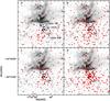 |
Fig. 10 Spatial distribution of the NIR counterparts of the YSOs identified according to four different indicators, as explained in the text, overlaid with the Ks image. Also drawn, a contour of the surface density of Ks sources. Only objects with Ks ≤ 13.5 (unlike Fig. 8, where Ks ≤ 16 has been used) have been selected. a) YSOs identified on the basis of their IRAC colours: red symbols for Class II sources, a large blue triangle marks the only Class I source; b) YSOs identified on the basis of their combined JH(HKs) [4.5] colours; c)JHKs sources exhibiting a colour excess; d) X-ray sources. A colour version of this figure is available in the on-line edition. |
3.6. Ks luminosity function of Pismis 24
K luminosity functions (KLFs) are valuable tools in constraining the IMF of young star clusters (Lada & Lada 2003, and references therein). Our SofI field is large enough to contain most of the cluster core members, so in principle it allows us to construct a KLF representative of the cluster. Unfortunately, nearby control field images are not available to correct for field star contamination as usually done. It would even be difficult to find a suitable field, given that we are nearly looking towards the Galaxy centre. Hence, we must resort to an alternative method in order to minimise contamination from field stars. This means using either colour intervals or the NIR counterparts of the X-ray sources to select the cluster population.
We followed Massi et al. (2006) to produce a dereddened KLF from sources with detections in the H and Ks bands. Each datapoint is shifted along the reverse reddening direction in the (H − Ks, Ks) space to a locus representative of the magnitudes and colours of young unextincted PMS stars. We adopted the locus they proposed without NIR excess correction (hereafter the pseudo-sequence) and shifted it to account for a distance of 1.7 kpc. We have also modified the upper part of the locus by adding one more segment (essentially a vertical line with H − Ks = −0.05 coinciding with the ZAMS; Koornneef 1983) to account for the most massive cluster members. Given that the cluster age is rather well constrained to ≲3 Myr (see Sect. 3.7) the method is particularly suited to obtain a reliable dereddened cluster KLF (as shown by Massi et al. 2006).
A few different selection criteria can be chosen to identify the cluster members. We showed in Sect. 3.3 that H − Ks ≲ 1 and J − H ≲ 2 enclose the cluster population in the NIR CCDs of Pismis 24. Alternatively, one can use the pseudo-sequence as a reference and pick all the sources inside a well-defined extinction interval from it. In principle one could choose the extinction range found in the visible, 3.2 <AV< 7.8 (Fang et al. 2012). However, Figs. 6c,d suggests that the cluster population may span a wider range in AV. Therefore, we will use the NIR counterparts of the X-ray sources to refine the extinction cuts.
Nevertheless, the reddening interval 3.2 <AV< 7.8 sets up an extinction-limited sample whose contamination from field stars is expected to be negligible, and we used it to perform a few statistical tests. In Fig. 11 we show four dereddened KLFs obtained by changing the most critical parameters (sampling field sub-region, distance, extinction interval). A simple χ2 test confirms the visual impression from Fig. 11 that the KLFs obtained are not statistically different if sources are selected from the whole SofI field or the southern field only, and proves that the dereddened KLFs do not change if the selected sources are further required to also have a valid J detection. By fitting a linear relation to the logarithmic KLFs between Ks = 6.5 and Ks = 13, one obtains a slope of 0.21 ± 0.05 (χ2 = 1.25), if the sources are picked from the southern field only, and 0.20 ± 0.09 (χ2 = 0.80), if a pseudo-sequence shifted to 2.56 kpc is used. Thus, even a large systematic error in distance do not change the shape of the KLF. Finally, the χ2 test indicates only a marginal difference between the KLFs obtained from sources in the 3.2 <AV< 7.8 and that obtained from sources in the AV> 7.8 mag extinction range; i.e., the effect of contamination of the KLF by field stars cannot be derived in a clear-cut, statistical way.
A rough estimate of the completeness limit for the KLF is (dereddened magnitude) Ks = 15. This can be derived from the Ks vs. H − Ks diagram as the dereddened magnitude of the point of intersection of the completeness limit locus (dashed line in Figs. 6c,d) with a pseudo-sequence extincted by a value equal to the upper limit in the sampling AV range. It can be seen in Fig. 11 that the limiting magnitude obtained lies roughly 1–2 mag below the KLF peak.
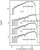 |
Fig. 11 Dereddened KLFs (see text) for sources in the H − Ks colour interval corresponding to a reddening interval 3.2 <AV< 7.8 (see text) from the mean locus (pseudo-sequence) of young stars. From bottom up: sample selected from the southern field only (pseudo-sequence at 1.7 kpc), from the whole SofI field (pseudo-sequence at 1.7 kpc), and from the whole SofI field (using a pseudo-sequence shifted to a distance of 2.56 kpc). The KLF at the top has been obtained for sources with AV> 7.8 mag picked from the whole field (pseudo-sequence at 1.7 kpc). The two vertical dotted lines mark the completeness limit for the KLF at the top (Ks = 13) and that for the other three KLFs (Ks = 15). |
The most critical issue in selecting a representative sample of cluster members by using a reddening interval is finding a suitable upper limit that allows including most of the population with only small contamination. As discussed in Sect. 3.4, the X-ray sources are mostly cluster members and their NIR counterparts can be used to construct a KLF completely independent of any assumption of a reddening interval. A comparison between the dereddened X-ray counterpart KLF and that from sources with 3.2 <AV< 7.8 is shown in Fig. 12 (pseudo-sequence at 1.7 kpc, data from the whole field). They are clearly different and a χ2 test on the segment from Ks = 6.5 to to 11.5 yields a significance level of 0.35, confirming they are only marginally consistent with each other. On the other hand, Fig. 12 shows that the dereddened KLF obtained from sources in the wider range 3.2 <AV< 15 looks more consistent with that from X-ray counterparts, which is confirmed by a χ2 test on the rising part of the distributions. The stars in the extinction range 3.2 <AV< 15 from the pseudo-sequence fall inside the less extincted datapoint concentration in the CCDs of Figs. 6a,b that mostly features cluster members. Thus, they make up a natural extension of the sample of X-ray counterparts, picking sources down to a fainter completeness limit in Ks.
As a final remark, we caution against the effects of the NIR excess of a fraction of cluster members. The selected extinction interval does not account for the NIR excess exhibited by a number of YSO. These YSOs are both brighter in Ks and look as if they were more extincted than their central stars actually are, hence they look more massive than they are. As discussed by Massi et al. (2006), this will result in a steeper KLF.
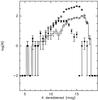 |
Fig. 12 Dereddened KLF (see text) for sources in the H − Ks colour interval corresponding to a reddening interval 3.2 <AV< 7.8 (see text) from the mean locus (pseudo-sequence) of young stars (histogram), for Ks counterparts of X-ray sources (full squares), and for sources in the reddening interval 3.2 <AV< 15 (open squares). All are obtained with the pseudo-sequence at 1.7 kpc and from the whole field. Error-bars are derived from Poisson statistics. |
3.7. Age of Pismis 24 and masses of stars from the optical HST data
Following Massi et al. (2006), if the age and star formation history of Pismis 24 are known then its KLF can be converted into an IMF. So far, the age of Pismis 24 has been estimated in two ways: from the age of the most massive stars and from the age of the intermediate to low-mass stars. Massey et al. (2001) compared the most massive cluster stars with isochrones in a Hertzsprung-Russell diagram finding a median age of 1.7 Myr and a very likely coevality. A similar exercise was done by Fang et al. (2012), who found that the age of the 6 most massive stars is between 1–2.7 Myr if they are assumed to be coeval. On the other hand, Fang et al. (2012) obtained optical spectra and RI photometry for 151 stars with an X-ray counterpart, deriving their spectral type and extinction. As expected, once dereddened these stars spread out well above the ZAMS locus in an R vs. R − I diagram, confirming their PMS nature. By comparing their location with PMS isochrones from Dotter et al. (2008), Fang et al. (2012) showed that their age distribution peaks at 1 Myr. Finally, Lima et al. (2014) obtained an older age of 5 Myr by fitting Padova isochrones in a J vs. J − Ks diagram.
We used our VI photometry from the HST/WFPC2 images to check the age derived by the other authors. The results are shown in the V vs. V − I diagram of Fig. 13a, along with the ZAMS locus and isochrones for PMS stars 1, 3, and 10 Myr old (for a reddening AV = 5.5 mag and a distance of 1.7 kpc). For the ZAMS, we have adopted V − I colours from Ducati et al. (2001) for B stars (transformed to the Johnson-Cousins standard), and from Bessell (1979, 1991) for later than B stars. We note that V − I colours from Ducati et al. (2001) and Bessell (1979) show a discrepancy of ~0.1 mag for B7 stars, although they are in good agreement for A0 stars. The PMS sequence of the cluster is easily identified above the ZAMS, and the stars fall in the age interval 1–10 Myr with an average of about 3 Myr. The 11 optical sources without a NIR counterpart (and an X-ray detection, either) mostly lie to the left of the ZAMS, as expected for field stars.
To further investigate the age dispersion, we show in Fig. 13b the Ks vs. H − Ks diagram for the NIR counterparts of the optical stars, along with the isochrones for PMS stars 1 and 3 Myr old (same reddening and distance as above). The NIR counterparts of the PMS stars with X-ray emission are shown as full triangles. By comparing the data with the isochrones, the PMS stars appear more massive in the NIR than at optical wavelengths. This discrepancy already appears if one compares the masses found by Fang et al. (2012) and by Wang et al. (2007). The latter authors found more massive counterparts for the X-ray sources from 2MASS NIR data. We tried estimating the PMS star extinction by shifting their datapoints along the reddening vector to the 1 and 3 Myr loci in the Ks vs. H − Ks diagram. When turned into optical extinction, this causes the stars to move to the upper corner of the V vs. V − I diagram of Fig. 13a, to the left of the ZAMS. Although a photometric error of 0.1 mag in the NIR would result in an error of ~1 mag in AV, the shift is much larger for most of the objects. This is evidence that the dispersion in the magnitude-colour diagram of Fig. 13b is due not only to differential extinction, but also to an infrared excess. Although only part of the stars exhibit an excess in the J − H vs. H − Ks diagram (i.e., lie below the reddening band of the MS; see Fig. 13c), a comparison between the NIR sources with X-ray counterparts and the locus of Classical T Tauri Stars (Meyer et al. 1997), also drawn in Fig. 13c, confirms that their spread in the CCD is strongly affected by NIR excess emission. Figure 13c also shows that the steepest of the extinction laws we considered, that of Straiz˘ys & Laugalys (2008), would only marginally increase the fraction of sources with a NIR excess.
Statistics of the detection of HST sources in infrared bands and X-ray.
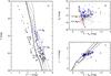 |
Fig. 13 a)V vs. V − I for stars towards Pismis 24 from HST/WFPC2 images. The full line marks the ZAMS, the dashed lines are isochrones for (from the right) 1, 3, and 10 Myr old PMS stars obtained from the evolutionary tracks of Palla & Stahler (1999). These have been reddened by AV = 5.5 mag and scaled to 1.7 kpc. The loci of 1 and 0.4M⊙ are labelled near the 1 Myr isochrone. Large open triangles are stars without a NIR counterpart, whereas small blue full triangles are stars with X-ray detection. b)Ks vs. H − Ks for the NIR infrared counterparts of the optical stars (red open squares: stars on the left of the optical ZAMS; full squares: stars on the right of the optical ZAMS; blue full triangles: stars on the right of the optical ZAMS also detected in X-ray emission). The full lines are the isochrones for (from the right) 1 and 3 Myr old PMS stars obtained from the evolutionary tracks of Palla & Stahler (1999), same reddening and distance as above. The loci of 1 and 0.4 M⊙ are also labelled and the dashed lines are their reddening paths (for 1 Myr old stars, up to AV = 10 mag, according to Rieke & Lebofsky 1985). c)J − H vs. H − Ks for the NIR infrared counterparts of the optical stars (same symbols as above, but stars on the left of the optical ZAMS are omitted). The full line is the unreddened MS, the dashed lines are reddening paths with crosses every AV = 10 mag, following Rieke & Lebofsky (1985). Also shown as full lines, the reddening paths according to the extinction law derived by Straiz˘ys & Laugalys (2008). The dot-dashed line marks the locus of Classical T Tauri Stars (Meyer et al. 1997). A colour version of this figure is available in the on-line edition. |
The issue can be better tackled by adding the IRAC 4.5 μm measurements to JHKs, using the criteria of Winston et al. (2007) to discriminate sources with a NIR excess, as done in Sect. 3.5. We found 49 HST stars with a detection in the 4.5 μm band, only 5 of which lie to the left of the ZAMS in Fig. 13a. A statistics of the detection of the optical sources in infrared bands and X-ray is shown in Table 6. The stars on the left of the optical ZAMS are referred to as field stars, whereas those on the ZAMS or to the right of it are referred to as cluster members. Clearly, 50% of the HST cluster members with V< 23 were detected at 4.5 μm, whereas this fraction drops to 32% for V ≥ 23. This is obviously a signature of incompleteness in the IRAC bands; in fact, Table 3 lists mass completeness limits in the 3.6 and 4.5 μm bands of 2 M⊙ for naked PMS stars and ~1 M⊙ for Class II sources. Out of the 44 HST cluster members with detection at 4.5 μm, 70% exhibit a NIR excess, a fraction increasing to 87% if considering only those with V ≥ 23. Hence, at least 27% of all the optically detected cluster members exhibit a NIR excess. Since PMS star emission is hardly affected by disk emission in the optical bands, the sample of HST cluster members is not biased towards stars with excess emission in the NIR, although limited by extinction. Therefore, this fraction may well be a lower limit for the fraction of cluster members as a whole with a circumstellar disk.
Figures 13b,c suggest that a large fraction of JHKs sources with X-ray detection must also exhibit a strong NIR excess (having ruled out heavy extinction). In fact, 59% of the HST cluster members with a detection in the 4.5 μm band also have an X-ray counterpart. Of these, 17 (65%) exhibit a NIR excess. Thus, a large number of cluster members must be associated with a circumstellar disk and are therefore quite young; the mass mismatch between optical and NIR CMDs would even increase by assuming an age of 10 Myr. Therefore, we think that the cluster age can be constrained to 1–3 Myr and the age dispersion shown in the V vs. V − I diagram is not real. No clear age patterns can be noticed by selecting stars falling in limited areas of the field, although those near the massive stars show a tendency to lie close the 3 Myr isochrone (however with a number of objects quite small).
The nature of the optical cluster members undetected in X-ray can be deduced from Fig. 13a. At the high-mass end, X-ray emitting sources are more numerous than at the low-mass end. The X-ray activity in PMS stars is known to be variable (see e.g., Flaccomio et al. 2012), so a fraction of low-mass stars in a phase of increased X-ray activity were detected. This clarifies why Fang et al. (2012) found RI counterparts of X-ray sources down to <0.4 M⊙, whereas the estimated mass detection limit in X-ray is higher (>0.7 M⊙; see Sect. 3.4). The optical cluster members undetected in X-ray are therefore lower-mass stars in a phase of lower X-ray activity.
Unlike intermediate to low-mass stars, the cluster massive members are Main Sequence (MS) stars. For MS isochrones the time is measured starting from the ZAMS, while PMS tracks use different zero-age reference isochrones; e.g. Palla & Stahler (1999) adopted their birthline. Classical PMS evolutionary tracks usually start from the Hayashi tracks rather than the birthline. Tognelli et al. (2011) followed this approach and showed that their tracks intersect the birthline before 1 Myr for almost all stellar masses. In particular, for M< 1.5M⊙ this happens before 0.5 Myr.
Birthlines, like that of Palla & Stahler (1999), necessarily join the ZAMS for stellar masses somewhere around 10M⊙, hence cannot be used as a zero-age isochrone for massive stars. So the results obtained from massive (MS) and intermediate to low-mass (PMS) stars simply suggest that most of the massive stars were already on the ZAMS when most of the intermediate and low-mass stars were still emerging from the birthline or were still contracting along a PMS track, within ~1 Myr from each other.
3.8. The initial mass function of Pismis 24
To convert dereddened Ks magnitudes in masses, we used the PMS evolutionary tracks computed by Palla & Stahler (1999), as in Massi et al. (2006). Since the relationship between Ks and stellar mass depends on age, we used isochrones for 2 different ages, 1 and 3 Myr respectively. As shown in the previous section, these encompass the range of mean ages derived for the cluster. At these ages, Palla & Stahler (1999) predict that intermediate mass stars are already on the ZAMS, so the isochrones have been complemented with a ZAMS model, as explained in Massi et al. (2006). We have further extended the ZAMS relationship up to O3–4 V stars by assuming these to have the same V − K colour as O6–9 V stars (given by Koornneef 1983). This should yield a good approximation for the mass of the OB members even though they have already departed from the ZAMS, also considering that the masses of early O stars (the most evolved ones) are highly uncertain (see Weidner & Vink 2010).
In addition, to test the effects on the IMF of adopting different models for massive stars to convert brightness into mass, we also used the synthetic tracks of Lejeune & Schaerer (2001) for main sequence stars from 0.8 to 100 M⊙, in particular the ones for solar metallicity (Z = 0.02), age 1 Myr and increased mass loss from high-mass stars. The Ks magnitudes of OB stars were, therefore, converted into initial rather than current masses. These tracks also allowed us to test the effect of using a MS Ks-mass relationship for all stellar masses, as opposed to our adopted mixed MS-PMS isochrones.
Finally, we note that a small range of intermediate masses is necessarily degenerate when using the PMS tracks of Palla & Stahler (1999), given that ZAMS stars and PMS stars of different masses overlap and exhibit the same Ks brightness in that range (lying around a value of a few solar masses). Thus, we cannot perform any mass conversion in that limited range and this explains the gaps in Fig. 14.
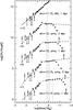 |
Fig. 14 Logarithmic initial mass functions obtained from the dereddened KLFs, each shifted by the amount indicated on the left. The assumed distance moduli, ages, and synthetic tracks (either PMS for low-mass stars, or MS for all stars) are also labelled. The dashed lines show the two-segment fits to the IMFs (for the IMF on the top, the full line is a fit to the whole distribution, which cannot be distinguished in the figure from the fit to the high-mass end only). The vertical dotted lines mark the mass for each distribution at the completeness limit of the corresponding dereddened KLF. |
Two-segment fits to the IMFs.
We show in Fig. 14 a set of IMFs obtained by sampling the whole SofI field in the reddening interval 3.2 <AV< 15 with respect to the pseudo-sequence. Given that we use 2MASS magnitudes for the brightest stars (saturated in our SofI images), massive binary stars (such as Pismis 24 1; see Maíz Apellániz et al. 2007) are not resolved. Thus the IMFs obtained are primary star IMFs. On the other hand, this allows us to make a direct comparison with most of the IMFs of clusters found in the literature, which are usually primary star IMFs, as well. We also show an IMF derived by assuming a distance of 2.56 kpc, which allows us to assess the effect on the IMF of a systematic error on distance.
All IMFs obtained using PMS tracks for low-mass stars exhibit a change of slope around M = 2.5 M⊙. This flattening does not depend on the sampling reddening interval, since it is also displayed by the IMFs derived from the KLFs of sources in the reddening interval 3.2 <AV< 7.8. We fitted the logarithm of the IMF from the PMS plus ZAMS tracks with two-segment functions; the slope of each one directly yields Γ (where dN/dlog M ~ Γ; i.e., for a Salpeter IMF, Γ = −1.3) in the fitting range. The brightest star (Pismis 24 1) is always omitted from the fits to the M> 2.5M⊙ part of the IMF, to avoid any biases due to its overestimated mass (for comparison, Maíz Apellániz et al. 2007 found 97M⊙, which in turn is an upper limit because of the double nature of this star). Adding this point results in a slightly flatter IMF with ΔΓ within 0.1–0.2 in all cases, which is inside the errors.
We list the results of our two-segment fits to the IMFs in Table 7, along with the fitting mass range and the reduced χ2. It has been shown (see, e.g., Maschberger & Kroupa 2009) that fitting straight lines to a histogram with bins of constant width leads to a biased result. Thus we also derived Γ for the high-mass end of the IMF by adapting the modified Maximum Likelihood estimator proposed by Maschberger & Kroupa (2009), along with their estimator for the upper limit of a truncated power law, in the hypothesis that the actual IMF is a power-law truncated at high masses. These results are also listed in Table 7 and, again, we do not include the brightest star in the computations. Its inclusion does not change significantly the obtained Γ, but of course it leads to an increase in the upper mass limit, by a factor ~2. To show how the choice of the KLF affects the results, Table 7 also lists fits to the IMFs from the dereddened KLF of stars selected in the reddening interval 3.2 <AV< 7.8.
A larger distance than that we have adopted yields higher stellar masses but does not affect Γ significantly. For masses ≲2 M⊙ the IMF flattens, except when using only MS tracks to convert brightness into mass. The flatter segment of the IMF extends beyond the completeness limit. In any case, by adopting the KLF of sources sampled in the range 3.2 <AV< 7.8, the completeness magnitude can be increased by ~1 mag, thus decreasing the corresponding mass value. The IMFs associated show a similar flattening, so there is no doubt that this is real, since this more conservative KLF is still expected to provide a representative sample of low-mass members.
Source counts inside selected areas in the SofI field of view.
To conclude, the cluster IMF appears to be scarcely affected by the choice of age and distance, the most significant changes being due to the choice of the underlying KLF and of the evolutionary tracks. Table 7 shows that by increasing the upper limit of the extinction range to select the cluster members from AV = 7.8 mag to AV = 15 mag one obtains a steeper IMF at the high mass end. Although using the MS tracks of Lejeune & Schaerer (2001) to convert Ks magnitudes into masses is a useful exercise, it is not appropriate for the low-mass cluster members since, as demonstrated in this work, they are mostly PMS stars. Its most notable effect is then on the MS high-mass part of the IMF, where nevertheless it only produces a slightly flatter distribution. This also allows one to assess the effect of an age spread, rather than a single burst of star formation, on the IMF: including a fraction of older PMS stars results in steepening the high-mass end of the IMF. On the other hand, the inclusion of cluster members with a NIR excess is likely to have steepened the IMF as a whole and, probably, also to have shifted the turning point towards a higher mass. Since stars with a NIR excess shift redwards in the Ks vs. H − Ks diagram, lowering the upper end of the reddening interval to AV = 7.8 mag should result in filtering out a large fraction of these objects. Thus, as a rule of thumb the actual slope of the high-mass end of the IMF should be bracketed by the values derived for the two extinction ranges we have considered.
Our data point to a Salpeter-like IMF, truncated to an upper mass limit of 50–100 M⊙. A flattening occurs at the low-mass end, with a turning point somewhere between 1–3 M⊙. If taken at face value, this flattening is consistent with the IMF prescribed by Scalo (1998), and the field star IMF of Kroupa et al. (1993). It is also consistent with the IMF of young clusters given by Chabrier (2003), although our data are unsuitable to investigate the log-normal part of this distribution.
4. Discussion
4.1. Star formation on the smaller scale: substructures in Pismis 24
Our NIR images allow us to study in more depth the core of Pismis 24. The SofI field of view covers an area containing what we have called, in Table 4, Pis24 core, Pis24N, and Pis24E, whereas Pis24W and Pis24S lie outside. Star N78 36 is visible in the northern part of the images along with the small associated cavity (more evident in the IRAC three-colour image of Fig. 2). However, only Pis24 core stands out in the contour map of Ks source surface density (Fig. 8). Apart from some doubts on Pis24N, both Pis24N and Pis24E are anyway characterised by a much lower surface density of IRAC sources than Pis24 core. Thus, they probably cannot be separated statistically from the background star counts in the smaller SofI field. If so, the value adopted for the surface density of field stars is overestimated and, consequently, the number of NIR sources associated with the cluster is underestimated. This is confirmed by the radial profile derived by Lima et al. (2014) for Pismis 24, which has a radius of ~3′.
One critical issue is whether the multiple density peaks of the core (see Fig. 8 and Table 5) represent real substructures or are rather the effect of variable extinction. Although the bulk of molecular gas lies in the SofI northern field, a few molecular clumps have been found projected towards the core (e.g., CO clumps E, F, and G of Massi et al. 1997, and CS clump D3 of Giannetti et al. 2012). However, some of these clumps appear red-shifted and those authors suggested that this is because these may lie in the rear part of the complex, accelerated away by rocket effect. In addition, the multiple density peaks are also clearly visible in the long exposure Spitzer images at 3.6 and 4.5μm, where extinction is much lower than in the Ks band (e.g., compare the SofI and IRAC images in Fig. 2). They are also well outlined by X-ray sources in Fig. 10. Thus, the subclustering of the core of Pismis 24 is probably real. Subcluster core NE (Fig. 8) lies between the elephant trunk and the massive stars, and all these structures are roughly aligned along the elephant trunk axis. Figure 10 highlights a large number of YSOs towards the Hii region, as well.
Whether this source distribution is the result of sequential star formation started by the massive stars in core C, with the youngest generation being the closest to the molecular gas, should be proven by demonstrating a corresponding age sequence. However, no clear trends are obvious from the HST photometry (see Sect. 3.7). Alternatively, the fraction of cluster members with a circumstellar disk is believed to be an indicator of the cluster age (Haisch et al. 2001). This fraction is derived by counting the number of members exhibiting a NIR excess. As already noted, not all the stars with a circumstellar disk exhibit a colour excess in a J − H vs. H − Ks diagram, so some data in at least one longer wavelength band are needed. We used our NIR-IRAC combined photometry (JHKs [3.6] [4.5]) and determined the number of NIR sources up to Ks = 13.5 which exhibit a NIR excess either in JHKs or in JH(HKs) [4.5] (or both). The upper limit in Ks was chosen to minimise incompleteness effects, following the results of Appendix E. Furthermore, we ruled out all sources with J − H> 2 in order to keep background giants out.
We counted the NIR sources distributed in five different areas: a rectangular one (~0.74 × 0.31 pc2) including the Hii region (G353.2+0.9), and four circular ones. Two of the circles coincide with subclusters core NE (radius ~0.11 pc) and core SW (radius ~0.14 pc), respectively (see Fig. 8), whereas subcluster core C has been further subdivided in two parts, one centred on the massive stars (SE, radius ~0.21 pc), the other including the north-western tip (NW, radius ~0.16 pc). The results are listed in Table 8.
The small number of IRAC-selected Class II sources in Table 8 obviously reflects the lower sensitivity of this photometry (see Sect. 3.5), given that Ks = 13.5 samples mostly intermediate-mass stars and only the brightest of the lower-mass Class II sources. The fraction of sources with a circumstellar disk that we find is always larger than the 27% obtained in Sect. 3.7, which is plausible (taking into account that 27% may be a lower limit). The results do not depend much on the source selection criteria. In fact we obtained only slightly smaller values by either including sources up to Ks = 15.5 or adding the further criterion 0.2 ≤ H − Ks ≤ 1. Therefore, the fraction obtained should not be affected significantly by lower mass stars whose brightness raises them above the adopted Ks = 13.5 limit due to their NIR excess. In conclusion, the fractions of star-disk systems in the five areas are consistent with each other within the errors and point to a global value between 0.3–0.6, which would imply ages between 2–4 Myr (Haisch et al. 2001), consistent with the inferred age of Pismis 24.
If the derived fractions were taken at face value, the area towards the Hii region would be younger than subcluster core C SE, which harbours the most massive stars in Pismis 24. Subcluster core C SE in turn would appear younger than the surrounding areas. However, a few sources of bias, as well, must be considered. The most massive stars, towards core C SE, are saturated in the SofI image and a few close-by fainter NIR sources could not be measured (we remind the reader, e.g., of the 15 X-ray sources without a NIR counterpart located close to the two most massive stars). On the other hand, the extinction gets higher towards the Hii region and the sampling of 4.5 μm sources gets worse.
The fraction of disk-star systems listed in Table 8 is consistent with those derived by Fang et al. (2012). However, we do not find evidence of a significant decrease towards the two most massive stars as they do. As we have shown, the computation has to accurately take into account the issues of completeness and contamination in the different bands.
More insight into the differences between subcluster populations can be gained by examining in detail all the sub-regions. This is done in Appendix F along with a discussion on a few individual objects. O-type stars are only contained in the south-eastern part of subcluster core C (except possibly one in core SW), whereas the most massive stars in the other subclusters are at most early B stars. Thus, there are no intense ionising sources inside the Hii region, as instead was suggested by Felli et al. (1990), who misplaced two NIR sources (see Appendix F). This conclusively rules out the scenario proposed by those authors, where the ionisation of the Hii region was due to embedded sources lying in the ionised gas. The extended cluster halo underlying the subclusters may be composed of low-mass stars drifting out of the core. For typical dispersion velocities of ~2 km s-1, one in fact expects to find stars up to ~4′ from the core of Pismis 24 in ~1 Myr.
Assuming that the subclustered structure is real, one might ask whether this can reflect inhomogeneities that were already present in the parental molecular cloud. Parker & Meyer (2012) performed numerical simulations of clusters of 1000 members, showing that sub-structured distributions with a radius of 1 pc collapse to a central concentration after 1 Myr if they are initially subvirial (i.e., with a virial ratio T/ | V | < 1). However, they remain sub-structured even after 5 Myr if they are originally supervirial (i.e., with a virial ratio T/ | V | > 1), as expected in case of fast gas removal. Since these supervirial clusters expand quickly, the presence of substructures within ~1 pc in the Pis24 core is consistent with a scenario in which a young (<5 Myr) stellar population formed in different nearby gas clumps, quickly dispersed by the ionising photons from the most massive stars. These clumps should have had sizes of the order of few 0.1 pc.
4.2. Star formation on the smaller scale: stellar population of Pismis 24
Although the massive members of Pismis 24 are main sequence stars, its low-mass members are PMS stars. This is typical of very young (~1 Myr) clusters; for example the Orion Nebula Cluster (Hillenbrand 1997), the centre of NGC 3603 (Stolte et al. 2004), or NGC 602 (Gouliermis et al. 2012). Whether O-type stars are the last stars to form in a cluster is still an open issue (Tan et al. 2014). This point of view is not at odds with the PMS nature of the lower-mass stars, provided that the growth of massive stars towards the ZAMS is very fast and takes only a small fraction of the cluster age. Russeil et al. (2012) estimated that the starless and protostellar phases in the development of massive stars in NGC 6334–NGC 6357 have statistical lifetimes of ~0.01 Myr and 0.1 Myr, respectively. If so, high-mass stars can form, grow and start their main-sequence phase while already-formed low-mass stars are still contracting towards the ZAMS.
As for the stellar content of Pismis 24, our derived IMF includes 11 (if 3.2 <AV< 7.8) to 22 (if 3.2 <AV< 15) stars with M> 14 − 15M⊙ (i.e., early B to early O stars), irrespective of the adopted age or evolutionary tracks. Massey et al. (2001) list 8 earlier than O9 stars in the cluster. Wang et al. (2007) review the total number of massive stars quoted in the literature and list 17 known earlier than B0 stars plus 13 candidate O stars based on their X-ray luminosity. Of these, 11 plus 4 lie inside the SofI field, which is consistent with the number from our derived IMF. Interestingly, most of the remaining high-mass stars are located south of Pis24 core, and may be associated with Pis24 S (see Fig. 5).
The number of stars in the cluster core down to 0.1 M⊙ can be derived from either the surface density of 3.6μm sources (see Table 4) or the surface density of Ks sources (see Table 5), by assuming the mass completeness limits obtained for an age of 1 Myr and the IMF prescribed by Scalo (1998). We found ~2300 stars from the counts at 3.6μm and ~350 stars from the counts in the Ks band. The difference is probably due to both contamination from Class II sources mimicking intermediate-mass star fluxes at 3.6μm, and an overestimate of the average field star density in the much smaller SofI field. Alternatively, the total number of members can be estimated from the high-mass end of our derived IMF. Considering that we have found 28 (for 3.2 <AV< 7.8) to 85 (for 3.2 <AV< 15) stars down to ~6.5 M⊙ (assuming an age of 1 Myr), a Scalo IMF yields ~3600 to ~11 000 members in the Sofi field. This is consistent with ~10 000 (in fact ~5000 if the distance is shortened to 1.7 kpc) found by Wang et al. (2007) by scaling their derived X-ray luminosity function (obtained from sources on a larger area than our SofI field) to that of the ONC. Thus, the stellar mass of Pis24 core amounts to ~2 − 6 × 10³M⊙ for a Scalo IMF. Lima et al. (2014) actually derive a lower mass, 533 ± 50 M⊙, which would imply that most of the cluster mass is in massive stars. Incidentally, this is the lowest mass estimate quoted in the literature; nevertheless it highlights how sensitive this numbers are to the decontamination technique adopted.
4.3. Star formation on the smaller scale: dynamical properties of Pismis 24
One interesting property of Pismis 24 is the possible early ejection of massive stars from the cluster. In particular, we note that the O-type star Pismis 24 13/N78 36 (see Fig. 2) is located on the opposite side of subcluster core C SE with respect to the O stars Pismis 24 2 and Pismis 24 3, all roughly aligned along a line passing through core C SE. The ejection of massive stars from clusters may happen due to three-body encounters, in which massive binaries are involved (see, e.g., Zinnecker & Yorke 2007). Massive stars located on a line roughly centred on the cluster core may indicate momentum conservation in one of these episodes. This should become clear by measuring their radial velocities. In addition, Gvaramadze et al. (2011), in a systematic search for runaway OB stars associated with NGC 6357, listed four other distant B0 to O V stars that may have been ejected from Pismis 24, three more B0 to O V stars that may have been ejected from AH03J1725-34.4, and one O6 V star possibly ejected from either of them. The Wolf-Rayet star WR93, 4′ east of Pis24 core, could have been ejected, as well (this would cause an age inconsistency according to some authors, but would not be an issue according to Massey et al. 2001). This early ejection of massive stars would indicate both that the early phases of the two clusters were highly dynamically unstable, and a high fraction of pristine binaries among massive stars. By the way, the two most massive members of Pismis 24 are known to be binary stars.
4.4. Star formation on the smaller scale: from gas to stars
To infer the properties of the gaseous environment from which Pismis 24 originated, we start by noting that, from Fig. 8, the most massive members of Pismis 24 lie at a projected distance ~ (~0.8 pc) from the ionisation front in the north. The gas facing these stars (with pillars, see Fig. 2) reminds one of the inner wall of the cavities in the simulations by Mellema et al. (2006) and Arthur et al. (2011). Pismis 24/G353.2+0.9 is also somewhat reminiscent of other young open clusters interacting with nearby gas such as NGC 602/N90 in the SMC (e.g., Gouliermis et al. 2012).
The molecular gas north of Pismis 24 is likely to be the remnant of a larger complex where the cluster was born. Giannetti et al. (2012), summarising both their own and previous observations, confirmed that the molecular gas is being eroded and pushed aside by the intense UV field. Hence, Pismis 24 has quickly cleared off its parental cloud, whose gas must have been ejected to the south through a champagne flow. A sketch of the primordial environment of the cluster could be the following. Let us assume that the Hii region has evolved in a medium of constant density with a radius equal to the distance between the most massive stars and the ionisation front (~1 pc). This would encompass all three subclusters of Fig. 8. If we take the age of the cluster (~1 Myr) as the age of this idealised Hii region, we can use Eq. (12:20) of Spitzer (1978) to derive the Strömgren radius (~0.02 pc). In turn, from the Strömgren radius we can derive the average medium density (nH ~ 106 cm-3). Such a cloud would have had a mass ~105M⊙. Gendelev & Krumholz (2012) showed that the ionisation front expands only slightly faster in a blister-type Hii region compared with a spherically-symmetric one, so this does not affect the final result significantly. Using the total stellar mass derived in Sect. 4.2, the star formation in this cloud would have occurred with an efficiency of ~2–6%. This efficiency is of the same order of that usually measured in molecular clouds as a whole (Padoan et al. 2014), but could be even larger if the stars formed in several clumps reflecting the current subclustered structure, hence with sizes less than a few 0.1 pc. In this case, the expansion of the Hii region could be delayed to match the cluster age by increasing the average clump density (embedded inside a lower density gas), by invoking UV radiation absorbed by dust (which would imply lower gas densities), or by gas inflow (Dale & Bonnel 2011). The remaining gas must have been quickly cleared via champagne flows. Some of the properties of the molecular clouds in the north should still reflect those of the cluster parental cloud. Giannetti et al. (2012) found that the molecular gas is distributed in clumps ~0.2 pc in size, with average densities n(H2) ~ 103 − 105 cm-3 and masses ~10 to few 100 M⊙ (once scaled to our assumed distance). The densest and most massive of them may be similar to those where the cluster stars formed.
Are there any hints that star formation in parts of Pismis 24 has been triggered by the feedback from the massive stars? Numerical simulations show that photo-ionisation from massive stars inside molecular clouds generally leads to a slight decrease in the global star formation efficiency, with gas expulsion partly compensated for by triggered star formation (e.g., Dale et al. 2012a,b). Nevertheless, they show that triggered star formation does occur, and amounts to a few% of the total cloud mass (see also Walch et al. 2011). Dale et al. (2012b) find that the association of young stars with gas structures such as shells or pillars, as occurs in NGC 6357, is a good but not conclusive indication of triggered star formation. We could not detect significant age differences in different areas of Pis24 core based on the fraction of stars with a circumstellar disk, that could have pointed to sequential star formation as well. However, this fraction appears to be at least marginally higher towards the Hii region where other indications of triggered star formation have been found. Figure 10 shows that young stars are embedded in the Hii region. The elephant trunk with the young star IRS 4 at its tip is another sign of possible triggering. As discussed in Appendix F, this region hosts less massive stars than subcluster core C which may be an effect of photo-ionisation (Dale et al. 2012b). Giannetti et al. (2012) found that many of the gas clumps in the north are virialised and/or exhibit possible compression from outside, which may lead to further star formation.
The elephant trunk with IRS 4 at the tip inside G353.2+0.9 suggests that the so-called “radiation-driven implosion” (see Bisbas et al. 2011 and references therein) may be under way. When an ionisation front crosses a dense clump, it generates a shock which compresses the clump making it collapse under some conditions. Westmoquette et al. (2010) in fact found evidence of a D-shock propagating into the elephant trunk. The numerical simulations by Bisbas et al. (2011) nicely show how pillars with newly-born stars at the tip can be produced by this mechanism. Interestingly, they found that more intense ionising fluxes should disrupt less dense clumps rather than make them collapse. However, these authors considered clumps whose masses (15 M⊙ at most) are much less than that of the elephant trunk (a few 100 M⊙ according to Giannetti et al. 2012), so their results cannot be easily compared with our observations. Alternatively, Gritschneder et al. (2010) showed that pillars may naturally arise in turbulent clouds exposed to UV radiation, which acts to enhance the initial turbulent density distribution. In conclusion, although we cannot conclusively prove that triggered star formation is in progress towards G353.2+0.9, this seems quite likely.
5. Conclusions
We have retrieved archival Spitzer/IRAC data and studied the young star population in the star forming region NGC 6357, located in the Galactic plane (d ~ 1.7 kpc). We complemented these data with new JHKs observations, archival HST/WFPC2 images, and CHANDRA X-ray observations available in the literature, and focused on the stellar population (age, IMF, evidence of multiple generations of stars) in the young open cluster Pismis 24, which is part of NGC 6357. Since the region is only few degrees from the Galactic Centre in projection, we had to carefully assess the various effects that can bias the results, in particular when comparing photometry from different instruments at different wavelengths. We showed that the Spitzer/IRAC photometry is confusion-limited and, at longer wavelengths, suffers from saturation in the areas with intense diffuse emission (i.e., from the UV-illuminated surface of molecular clouds). We also showed that the JHKs photometry, Spitzer/IRAC photometry and high-resolution X-ray observations do not sample the stellar population homogeneously, but are complete only down to different stellar masses. In the case of Spitzer/IRAC photometry, the completeness gets even worse when including either of the bands at 5.8 and 8.0μm. Having considered all these effects, we obtained the following results:
-
1.
The Spitzer/IRAC photometry on the large scale shows anothertwo stellar clusters associated with NGC 6357,i.e., the cluster AH03J1725–34.4 (associated with theHii region G353.1+0.6), and the cluster we named“B” (associated with the Hii region G353.2+0.7).Class II sources (identified from IRAC colours)also cluster towards these three sites, suggesting a stellarpopulation of very young stars in all three cases. All have sizesof ~2.5 pc and exhibit subclustering on scales down to 0.5–1 pc. We estimated total numbers of stars of a few hundreds in each cluster down to the completeness limit. If the cluster ages are roughly the same (assumed ~1 Myr), the stars are counted down to ~2 M⊙ and all three clusters must contain similar total numbers of members.
-
2.
Both Pismis 24 and AH03J1725–34.4 lie inside cavities where they appear off-centred, interacting with molecular clouds to the north. Cluster B lies inside a cavity, as well.
-
3.
We discussed briefly the NIR extinction law towards Pismis 24, concluding that the one derived by Rieke & Lebofsky (1985) should be appropriate. The J − H vs. H − Ks diagram indicates a large population of extincted giant stars, which is expected given that we are looking towards the innermost parts of the Galaxy.
-
4.
The NIR photometry shows that the core of Pismis 24, itself one of several other substructures, contains three surface density peaks, which are likely to represent real subclusters. All the most massive members lie in the same subcluster, whereas only intermediate- to low-mass members populate the other subclusters.
-
5.
Optical HST photometry confirms a cluster age of ~1–3 Myr. However, we found that many of the NIR counterparts of the optical stars (those with X-ray detection in particular) appear more massive than from optical photometry. This points to a large fraction of stars exhibiting a NIR excess.
-
6.
We derived from their NIR excess (evaluated including the IRAC 4.5 μm band) the fraction of stars with a circumstellar disk and this is in the range 0.3–0.6, consistent with an age ≲4 Myr. We found no decrease of this fraction towards the massive stars.
-
7.
We derived the IMF towards the core of Pismis 24 by using K luminosity functions. We minimised contamination by field stars by selecting HKs sources in two different extinction ranges with respect to a pseudo-sequence of young stars, i.e. 3.2 <AV< 7.8 (derived from optical spectroscopy) and 3.2 <AV< 15 (derived from the NIR counterparts of X-ray sources). We found an IMF consistent with a Salpeter one down to ~2.5 M⊙. For M ≲ 2.5M⊙, the IMF flattens.
-
8.
Assuming the IMF prescribed by Scalo (1998), we estimated that Pismis 24 contains ~3600 to ~11 000 stars (2 − 6 × 10³M⊙), depending on the extinction interval used to select the cluster members.
-
9.
There are indications of triggered star formation towards the Hii region G353.2+0.9, where the UV radiation from the core of Pismis 24 interacts with the molecular cloud. We confirmed the results of Giannetti et al. (2012), who ruled out the scenario proposed by Felli et al. (1990) in which the ionising sources of G353.2+0.9 are embedded massive stars inside the Hii region itself. In fact, we did not find any stars earlier than B-type in the area.
-
10.
There are indications of an early ejection of massive stars from the core of Pismis 24, suggesting a dynamically unstable environment after gas expulsion.
-
11.
We proposed a picture of the molecular gas where the core of Pismis 24 formed. It must have been a dense (average n [H2] ~ 5 × 105 cm-3) cloud, ~1 pc in radius. Or, most probably, a group of denser clumps (n [H2] > 5 × 105 cm-3) ~0.1 pc in radius, embedded in a lower density gas (n [H2] < 5 × 105 cm-3).
Note added in proof. A new paper (Townsley et al. 2014), published after this one was submitted, presents further CHANDRA X-ray observations of NGC 6357, considerably enlarging the area surveyed by Wang et al. (2007). These observations can be summarised as follows: 800 X-ray sources are detected towards each of the three large clusters (Pis 24, A and B), confirming that they are very young clusters with a comparable number of members. Interestingly, diffuse X-ray emission is also found, pointing to hot plasma filling the various cavities that are present in NGC 6357.
Online material
Appendix A: Spitzer/IRAC data reduction
We downloaded all the basic calibrated data (BCD) and corrected BCD (CBCD) products, which were provided by the Spitzer Science Center through their standard data processing pipeline version S18.18.0. Data obtained from S18.18.0 need to be corrected in the 5.8 and 8.0 μm bands due to an error in calibration, so they have been multiplied by 0.968 and 0.973, respectively, following the prescriptions given in the web page4. For each raw image, the pipeline produces a flux-calibrated image (BCD), where all well-understood instrumental signatures (e.g., muxbleed) are removed (and including dark-subtraction and flat-fielding). The pipeline also attempts to systematically find all saturated point sources in the images and fit them using an appropriate PSF that is matched to the unsaturated wings of the source. A dedicated software module replaces the saturated point source with an unsaturated point source that has the correct flux density of the point source. We checked that this works quite well on the short-exposure frames but not on the long-exposure ones. Another pipeline module performs artefact correction (stray light, saturation, muxstripe, column pulldown and banding) on the BCD files, creating “corrected” BCD (CBCD) files. For details, see the on-line instrument handbook5.
The observations were performed in high dynamic range (HDR) mode, i.e., two images were taken at each position, a short exposure one (0.4 s) and a long exposure one (10.4 s). This allows one to also obtain photometry for bright sources avoiding saturation. The observed area was covered by using the IRAC mapping mode, with a grid of 10 × 8 positions in “array” coordinates, spaced by 260″ (i.e., slightly less than the detector size) in both directions defined by the detector axes. The selected dithering mode was “cycling”, with a scale factor “medium” and a number of positions equal to 5, i.e., for each grid position, 5 pairs (the short- and long-exposure integration) of dithered images were taken, randomly distributed up to a maximum distance of 119 pixels and with a median distance of 53 pixels. Therefore, most of the points in the mosaic result from the overlap of up to five images, although small areas can be covered by more than 5 images (where the dithered patterns of adjacent grid positions overlap) and few smaller areas may be covered by less than 5 images.
Mosaicking and co-adding of all frames were carried out by using MOPEX version 18.4.9, yielding a pair of larger images (short- and long-exposure) per band with a pixel size  (about half the native pixel size). We used a dual-outlier rejection strategy with conservative settings and experimented different values of the parameter RThreshold. The long-exposure CBCD frames at 5.8 and 8.0 μm displayed intense stripes associated with bright sources, absent in the corresponding BCD frames. We found out that these are features caused by the artefact-mitigation pipeline. Consequently, we constructed the long-exposure 5.8 and 8.0 μm images using the BCD files rather than the CBCD ones. On the other hand, as for the short-exposure mosaics, only a few CBCDs at 8.0 μm were found heavily affected by the problem and replaced by the corresponding BCDs. In all other cases we used the CBCDs.
Appendix B: Spitzer/IRAC photometry
We checked that any artefact had been removed efficiently from the final mosaicked images, except for the bandwidth effect in the long-exposure 5.8 and 8.0 μm ones. This gives rise to ghosts associated with the brightest sources. However, the corresponding artefacts were clearly recognisable and removed from the final point-source photometry. Some optical banding, as well, due to internal radiation scattering in the arrays, is present in the long-exposur 5.8 and 8.0 μm images yielding a small faint halo around the brightest areas. Being a diffuse structure, however, it is not expected to affect the final photometry significantly.
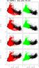 |
Fig. B.1 Magnitude–colour diagrams showing the magnitude in the various IRAC bands of the sources from the sample obtained in this work (black dots) as a function of [4.5] – [8.0]. Panels on the same row display, from top to bottom, the measurements for these sources in the 3.6, 4.5, 5.8, and 8.0 μm bands, respectively. In the left column panels, the sources from our sample are overlaid with those from GLIMPSE II (red dots). The green dots in the right column panels are those remaining from our photometry list after removal of sources contaminated by PAH emission. Only objects detected in all four bands with photometric errors <0.3 mag are plotted. |
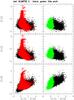 |
Fig. B.2 Magnitude–colour diagrams showing the magnitude of all sources from the sample obtained in this work (black dots) only detected in the first three wavelength IRAC bands (i.e., 3.6, 4.5 and 5.8 μm). Panels on the same row display, from top to bottom, the measurements for these sources in the 3.6, 4.5, and 5.8 μm bands, respectively, plotted as a function of [4.5] – [5.8]. In the left column panels, they are overlaid with all sources from GLIMPSE II (red dots) at least detected in the three shorter wavelength bands. The green dots in the right column panels are the sources remaining from our photometry list after removal of those contaminated by PAH emission. Only objects with photometric errors <0.3 mag in the three shorter wavelength bands are plotted. |
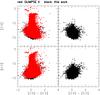 |
Fig. B.3 Magnitude–colour diagrams showing the magnitudes of all sources from the sample obtained in this work (black dots) only detected in the two shorter wavelength IRAC bands (i.e., 3.6 and 4.5μm). Panels on the same row display, from top to bottom, the measurements for these sources in the 3.6 and 4.5μm band, respectively, plotted as a function of [3.6] – [4.5]. On the left column panels, they are overlaid with all sources from GLIMPSE II (red dots) at least detected in the two shorter wavelength bands. Only objects with photometric errors <0.3 mag in the two shorter wavelength bands are plotted. |
Photometry was performed both on the short-exposure images and on the long-exposure ones. In each band, we set a saturation limit to the long-exposure mosaic, conservatively derived by estimating the saturation limit in a single BCD following the IRAC instrument handbook. The measured fluxes were converted into magnitudes by using the zero magnitude flux densities given in Table 4.1 of the IRAC instrument handbook (also given in Reach et al. 2005). The errors were calculated by using Eq. (7) of Reach et al. (2005), i.e., neglecting electronic noise. We discarded a number of residual false detections by visual inspection of the images, while others were subsequently removed by operating a colour-based selection during the analysis.
Short- and long-exposure photometry were matched in each band, adding the bright sources from the former to the faint sources from the latter according to the following criterion. We estimated a magnitude threshold for each band by requiring both that the average signal to noise ratio at the shorter exposure time was high enough, and that its corresponding flux was well below the single BCD saturation limit set at the longer exposure time. The sources with flux above the threshold were then taken from the short-exposure photometry, whereas those with flux below it were taken from the long-exposure photometry. The chosen thresholds are [3.6] = 10.5, [4.5] = 10, [5.8] = 8 and [8.0] = 8.5.
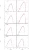 |
Fig. B.4 Number of sources per magnitude bins of 0.5 mag, from our database (black line) and the GLIMPSE sample (red line). The boxes in each row refer to the band indicated on the upper left corner. For the diagrams on the left column we used the sources detected in all four IRAC bands with photometric errors <0.3 mag, whereas for those on the right column we used all sources detected in at least the corresponding band (with photometric errors <0.3 mag in that band). |
We cross-checked the photometry from the long- and short-exposure mosaics in each band I by computing the difference in magnitude of all sources retrieved in both of them (with photometric uncertainties less than 0.3 mag). We plotted the histogram of the difference Δm between long- and short-exposure measurements in bins of 0.5 [I]-magnitudes, sampling the sources over two different image test areas. One area was chosen well inside the large ring-like structure (hence with little diffuse emission) and the other one inside the G353.2+0.9 projected area (with the most intense diffuse emission). For brighter magnitude bins, the histograms appear to peak at values that are within 0.05 mag from 0 (with a trend of the long-exposure measurements to be brighter) following distributions resembling Gaussian curves. However, when moving towards fainter magnitudes, the distributions become less peaked, their width increases, and a wing develops on the side where long-exposure measurements are brighter than short-exposure ones. The dispersion around the peak is always narrower than the typical photometric error inside each magnitude bin, This flatter distribution in the faint bins is more evident towards the test area with large diffuse emission, although it does not seem to be correlated with the presence of diffuse emission. This may be due either to the short-exposure photometry being nearer to its sensitivity limit, and/or to a better sampling of the sky around point-sources for longer exposures (i.e., better signal-to-noise). In addition, the distributions for the 8.0 μm band do not exhibit the wing and are narrower than in the other bands. It appears that we used a DAOFIND finding threshold larger at 8.0 μm than in the other bands, in units of one sigma of effective noise, leading to a smaller overlap between short and long exposures.
Whatever caused this trend in the distributions of magnitude difference, the difference between long- and short-exposures is of no concern at all at bright magnitudes (where the final photometry is taken from the short-exposure mosaics), while we assume that anyway the fainter fluxes are better characterised in the long-exposure mosaics (yielding higher signal to noise ratios).
A few sources (much less than 1% of the total) exhibit large differences between short- and long-exposure magnitudes (larger than 2–3 times the width of the Δm distribution). In most cases, either they fall on some artefacts in one of the two mosaics or they are residual cosmic rays passing the outlier rejection stage of MOPEX. These sources were either removed or were assigned a photometric estimate from the image unaffected by the artefact. This further confirms that residual contamination from artefacts or cosmic rays is very low, well below ~1% of the total sample in each band.
Another consistency test that we performed consisted in comparing the photometry from this work with that from the GLIMPSE survey. We retrieved all sources from the GLIMPSE II (epoch 1) archive within 30′ from RA = 17h25m and Dec = −34°18′. The area covered by our data is smaller than that and lies well inside the 30′ radius. In the magnitude-colour diagrams of Fig. B.1 showing magnitudes vs. [4.5] – [8.0], we have overlaid (left column) the GLIMPSE datapoints (red) and those from this work (black). We have selected only objects detected in all four bands with photometric errors <0.3 mag from the two samples. It appears that the two photometry lists as a whole are consistent with each other, apart for a large group of sources with [4.5] – [8.0] >2 much more numerous in our sample. These are sources contaminated by PAH emission arising in the bright filaments that cross the region (see Appendix D). When these objects are filtered out as explained in Appendix D, the remaining ones (green dots, in the right column boxes) are distributed in the mag-colour diagram like the GLIMPSE datapoints.
We repeated the same test by selecting all sources from our database with detections only in the first three bands (3.6, 4.5 and 5.8 μm). In the magnitude–colour diagrams of Fig. B.2 their magnitudes are plotted vs. [4.5] – [5.8]. We have overlaid these (in black) with (boxes in the left column) the GLIMPSE datapoints with detections in at least the first three bands (red). We have selected only objects with photometric errors <0.3 mag in the three shorter wavelength bands from the two samples. In this case the two photometric lists appear to be consistent, as well, apart from a slight excess of red sources in our sample with respect to the GLIMPSE sample. By removing all sources contaminated by PAH emission as explained in Appendix D and plotting the remaining ones (green dots, boxes in the right column), the excess of red sources disappears, confirming its origin. We note that the brightest sources in our sample with detection only in the first three bands have a magnitude ~10 in all bands. Since stars have colours ~0 mag in all IRAC bands, this indicates that the sources with detections only in the three shorter wavelength bands are mostly stars too faint to be detected at 8.0 μm, where the sensitivity is [8.0] ~ 10 − 12 (see bottom row of Fig. B.1).
Finally, in Fig. B.3 we plot magnitudes vs. [3.6] – [4.5] for all sources from our database with detections only in the first two bands and photometric errors <0.3 mag (black dots). These are overlaid (boxes in the left column) with datapoints from the GLIMPSE sample with detection in at least the first two bands (red dots). The two photometric lists appear again to be consistent with each other. The brightest sources from our database are a bit fainter than those in Fig. B.2, suggesting that sources detected only in the first two bands are again mostly stars too faint to be detected in the two longer wavelength bands.
One striking thing that appears clearly from Figs. B.1–B.3 is that the sensitivity limits of our photometry are about the same as those of the GLIMPSE photometry. Nevertheless, our photometry does result from images integrated at least for 10.4 s and, on average, corresponding to a total exposure time of 52 s. On the other hand, the GLIMPSE II (epoch 1) photometry is produced using two images per position with exposure times 1.2 s each. This property of the limiting sensitivities is demonstrated in Fig B.4, comparing histograms of number of sources grouped in 0.5 mag magnitude bins from our sample (black) and the GLIMPSE one (red). For the diagrams on the left column, we have used only the sources detected in all four bands with photometric errors <0.3 mag, whereas for the diagrams on the right column we have used all sources detected in at least one wavelength band (with photometric errors <0.3 mag in that band). In any case, the distributions from the two samples are about equal, except for the different number of sources retrieved (as said the selected GLIMPSE field is larger than the target one). Both exhibit an increase in the number of sources starting from low magnitudes, a turn off roughly at the same magnitude, and a steep decrease. This clearly indicates that the completeness limit (and the sensitivity limit) in each band is roughly the same for the two samples.
We noticed a similar effect when comparing our short- and long-exposure photometry. The latter is about one magnitude (1.5 mag at 5.8 μm) deeper than the former, although the sensitivity values listed in the IRAC handbook would suggest a difference of at least 3–4 mag. This means that our photometry is limited by a source of noise that does not depend on the integration time. This can only be confusion due to the large number of sources in the field, given that we are observing along a line of sight close to the Galactic Centre. This is confirmed by Ramírez et al. (2008) who, in their IRAC survey of the Galactic Centre, found that their photometry is limited by confusion, as well. Using images with average total integration time of 6 s, they quote completeness limits which are even less than those we can infer from Fig. B.4 for the GLIMPSE sample (with 2.4 s total exposure time). The histograms of number of sources vs. magnitude that they show, exhibit the same abrupt turn-off at the faint end as ours. Furthermore, Fang et al. (2012) achieve only slightly better sensitivities compared to GLIMPSE using IRAC images of NGC 6357 of 10.4 s exposure time. Therefore, we can conclude that our photometry is limited by source confusion.
Appendix C: Completeness of Spitzer photometry
The photometric completeness in a band (i.e., the capability of retrieving most of the sources up to a given magnitude in a field) mainly depends on the sensitivity of the observations in that band. Because the sensitivity attained in the four IRAC bands is different, the completeness limit is fainter in the first two bands and gets brighter by requiring simultaneous detection in more than one band. To study the effect, we constructed histograms of the magnitude distribution, in bins 0.5 mag wide, adopting several different selection criteria. All histograms display an increase in the number of sources N with increasing magnitude up to a peak, and a subsequent decrease due to loss of completeness. A few examples are shown for all bands in Fig. C.1. In the following, by “good” detection we will mean one with a photometric error <0.3 mag. In addition, by “completeness degree” we will mean the fraction of sources of a given magnitude (irrespective of their nature) that are retrieved in the field.
 |
Fig. C.1 Number of sources retrieved in the I band vs. [I] in bins of 0.5 mag. The boxes in each row refer to the Spitzer/IRAC band I indicated on the upper left corner of the left-hand box. Upper two rows: in the left column, we compare the I-band sources detected in all IRAC bands with photometric errors <0.3 mag (black line), and the sources detected in at least the first two IRAC bands with photometric errors <0.3 mag (red line); in the right column, we compare all sources detected in at least the first two IRAC bands, with photometric errors either <0.3 mag in both bands (black line), or <0.3 mag in at least the considered band I (blue line). Lower two rows: in the left column, we compare the I-band sources detected in all IRAC bands, with photometric errors either <0.3 mag in all bands (black line), or <0.3 mag in at least the considered band I (red line); in the right column, we compare the I-band sources detected in all IRAC bands, with photometric errors <0.3 mag in at least the considered band I (black line), and the sources detected in at least the considered band I with photometric errors <0.3 mag (blue line). |
To derive the completeness degree as a function of magnitude, we first compared the histograms obtained in each IRAC band from the following two samples of sources (see the left column in Fig. C.1). The first sample (S1) contains all the sources retrieved in a band I with simultaneous good detections in all 4 bands. The second sample (S2) contains all the sources retrieved in a band I with good detections in I and in at least one adjacent band. Hence, different samples S2 can be obtained depending on the choice of the adjacent band (e.g., we used 3.6 and 4.5μm for each of these two bands, 5.8 and 4.5μm for the 5.8μm band, and 5.8 and 8.0μm for the 8.0μm band). Hereafter, we will refer to the distribution of magnitude [I] for samples S1 and S2 as S1[I] and S2[I], respectively. At their peak, the distribution of S1[3.6] and S1[4.5] are a factor ~0.6–0.7 of that of S2[3.6] and S2[4.5], respectively. This ratio increases to >0.8 one magnitude below (i.e., brighter than) the peak.
The distributions of S1[8.0] and S2[8.0] (not shown) are qualitatively similar, although the ratio S1[8.0] to S2[8.0] is ~0.72 one magnitude below the peak of S1[8.0]. However, such a comparison is less significant than for other bands, given that most of the sources without a detection in any of the first two bands are probably just blobs of diffuse emission rather than stellar objects.
Based on the histograms of the magnitude distribution for sources with good detections in at least two bands (i.e., S2[I]), we conservatively estimate that the 80% completeness limits of each sample S2 lie roughly one magnitude below its distribution peak (set CL0). E.g., [3.6] = 12.25, and [4.5] = 12.25. Therefore, based on the above assumption, we can derive ~80% completeness limits for sources with good detections in all IRAC bands (set CL1): [3.6] = 10.25, [4.5] = 9.75, [5.8] = 9.25, and [8.0] = 8.75. These are obtained simply by measuring the magnitude at which the ratio of the distribution S1[I] to S2[I] is ~0.8, considering that this usually occurs more than one magnitude below the peak of S2[I] (hence where S2[I] has been assumed to be almost complete).
Estimated completeness limits.
The same exercise, but replacing the samples S1 with other samples obtained by requiring that the selected sources are detected in at least the first three bands with photometric errors <0.3 mag (S1a), yields the following 80% completeness limits (set CL2): [3.6] = 11.75, [4.5] = 11.5, and [5.8] = 10.25.
Requiring that all the sources in a given band be also detected in other bands with photometric errors <0.3 mag can be quite a demanding prescription, causing otherwise good detections in that band to be removed because the detection in just another band has an error >0.3 mag. We checked that this is only a minor problem by noting the following. The histograms of the magnitude distribution obtained by selecting I-band sources detected in all four bands, but requiring good detections in all bands for one histogram (S1[I]) and at least in the I band for the other (S4[I]), both peak at the same magnitude, irrespectively of I. The ratio S1[I] to S4[I] slightly decreases with increasing magnitudes down to >80% at the peak. The same is found by selecting I-band sources detected in the first three bands, but either requiring good detections in all three bands (S1a[I]) or at least in the I band (sample S6[I]). In this case, the ratio of the distribution S1a[I] to S6[I] is >75% at the peak. For I = 3.6 and I = 4.5μm bands, we compared the histograms of I-band sources with good detections in at least the first two bands (S2[I]) and I-band sources detected in at least the first two bands but with good detection in at least the I band (sample S8[I]). These histograms (see the two upper rows in the right column of Fig. C.1 are very similar each other, with ratio of distribution S2[I] to S8[I] > 95% at the peak. By replacing the distribution S8[I] with those of sources with at least a good detection in one of the first two bands (S8[3.6] ∪ S8[4.5]), the ratio decreases to > 86% at the histogram peaks. Therefore, the effect of requiring good detections in at least the first two bands should imply a completeness limit not too different from that in each single lower-wavelength band.
The lower two rows of Fig. C.1 show that 5.6 and 8.0 μm-band sources with at least a good detection in the considered band, peak at slightly lower magnitudes than the corresponding sub-sample obtained by requiring a good detection in all bands. As said, we believe that most of the sources in the two upper-wavelength bands without simultaneous detections in the first two bands are mostly blobs of diffuse emission or even artefacts. So the statistics of all detections (multiple as well as single) in those bands is very likely to be biased.
Finally, we expect quite different completeness limits in areas without and with diffuse emission. To test this, we repeated all experiments described above but by selecting 1) only sources contained in an area with at most faint diffuse emission, i.e., inside the large ring; and 2) only sources inside the area containing G353.2+0.9. There is no difference in the histogram peak locations for the sets CL0, CL1, and CL2, at 3.6 and 4.5μm, between the complete samples discussed above and those of the sources inside the ring. On the other hand, the peaks of the histograms for 5.8 and 8.0μm sources inside the ring shift to larger magnitudes. This is probably because the crowding of sources far from diffuse emission areas is much less severe in the two longer wavelength IRAC bands. Apparently, in the first two bands the total (i.e., with sources from the whole field) samples are dominated by sources not falling towards diffuse emission, hence by crowding effects.
As far as sources inside the area containing G353.2+0.9 are concerned, the peaks of the histograms shift to lower magnitudes for sets CL0, CL1, and CL2, as expected, excluding CL1 at 3.6 and 4.5 μm whose peaks are one magnitude above (i.e., fainter than) those of the total samples. We suspect that this is due to the chance associations of faint sources in the first two bands and blobs of diffuse emission in the two upper-wavelength bands, artificially increasing the detection efficiency when requiring good detections in all bands. In any case, the source statistics is quite poor. Thus, we believe that only the estimates from CL0 (i.e., from the first two bands) are reliable in areas of intense diffuse emission.
The derived completeness limits (at a 70–80% level) for different detection requirements and areas in the images are listed in Table C.1.
Appendix D: Contamination of YSOs due to other red sources in the Spitzer photometry
Figure B.1 clearly shows a prominent group of sources with [4.5] – [8.0] > 2 in our sample, much more numerous than in the GLIMPSE sample. This is better evidenced in Fig. D.1, by plotting [3.6] and [8.0] vs. [5.8] – [8.0] for sources detected in all four bands and having photometric errors <0.3 mag. The [4.5] vs. [5.8] – [8.0] plot (not shown) is similar to the [3.6] vs. [5.8] – [8.0] one, whereas the [5.8] vs. [5.8] – [8.0] plot (not shown) is similar to the [8.0] vs. [5.8] – [8.0] one. A population of red sources centred at [5.8] – [8.0] ~1.7–1.8 is quite easily identified. These sources appear to be faint at 3.6 and 4.5 μm (<10 mag), but bright at 5.8 and 8.0 μm (>10 mag). On the other hand, the group of sources centred at [5.8] – [8.0] ~ 0 are mostly stars.
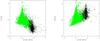 |
Fig. D.1 Magnitude vs. [5.8] – [8.0] in the 3.6 μm (left) and 8.0 μm (right) bands for all sources in our sample with detections in all four bands and photometric errors <0.3 mag (black dots). Overlaid (green dots), all remaining sources after removal of the various contaminants as explained in the text. |
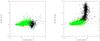 |
Fig. D.2 [3.6] – [4.5] vs. [5.8] – [8.0] (left) and [4.5] – [5.8] vs. [5.8] – [8.0] (right) for all sources in our sample detected in all four bands with photometric errors <0.3 mag (black dots). Overlaid (green dots), all remaining sources after removal of the various contaminants as explained in the text. |
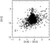 |
Fig. D.3 [8.0] vs. [5.8] – [8.0] for all sources in our sample only detected at 5.8 and 8.0 μm. |
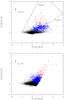 |
Fig. D.4 IRAC colour–colour diagrams. Top panel, [3.6] – [4.5] vs. [5.8] – [8.0] for sources detected in all four bands and with photometric errors <0.3 mag. Bottom panel, [3.6] – [4.5] vs. [4.5] – [5.8] for the same sources as above, plus those only detected in the three shorter wavelength bands (with photometric errors <0.3 mag). The two samples have been cleaned of contaminants as explained in the text. Following the prescriptions of Gutermuth et al. (2009) for their identification, Class I sources are in red and Class II sources in blue. Stars are marked as black dots. A reddening corresponding to AV = 20 mag (according to Indebetouw et al. 2005) is marked by an arrow. In the top panel, the regions occupied by Stage I and Stage II sources (Robitaille et al. 2006) are also outlined. |
Plotting the position of the sources with [5.8] – [8.0] > 1 on each of the IRAC images, we found that almost all appear to concentrate towards the filaments and areas of diffuse emission, whereas sources with [5.8] – [8.0] < 1 are anti-correlated with those areas. This suggests that most of the red sources are likely to be sources contaminated by PAH emission rather than actual intrinsically red objects. In fact, Zavagno et al. (2006) found that analogous filaments in RCW 79 have colours [3.6] – [4.5] ~0.1 and [5.8] – [8.0] ~ 1.8. The same average colours can be derived from Fig. D.2 for the red sources in our sample. These red sources probably arise due to random association of faint sources in the two shorter wavelength bands and bright blobs of diffuse emission in the two longer wavelength bands. All these blobs are bright, because of both the lower sensitivity and saturation problems towards those areas. Figure D.2 (right panel) shows well this datapoint population, whose colour [5.8] – [8.0] is remarkably constant (~1.7–1.8 mag) whereas [4.5] – [5.8] spreads between ~1 and ~4. In other words, there is a sort of break between the emission at 3.6 and 4.5 μm ([3.6] – [4.5] ~ 0) and that at 5.8 and 8.0 μm ([5.8] – [8.0] ~1.7–1.8 mag), which points to a random association rather than intrinsically red objects, as well.
A plot of [8.0] vs. [5.8] – [8.0] is shown in Fig. D.3 for sources only detected at 5.8 and 8.0μm; again, they are mostly concentrated at [5.8] – [8.0] ~1.7–1.8 and are distributed like the red sources in Fig. B.1. Spatially, they concentrate towards filaments and diffuse emission areas, as well. If they had counterparts in the two lower wavelengths, they would correspond to even redder sources (so red to remain undetected at those wavelengths because lying below the sensitivity limits) than those with detections in all four bands. Consequently, it is more plausible that the objects exhibiting [5.8] – [8.0] ~1.7–1.8 are mostly blobs of diffuse emission.
To understand why this population of red sources is scarcely represented in the GLIMPSE survey (see Fig. B.1), we plotted the position of all GLIMPSE sources detected in all four bands with photometric errors <0.3 mag. Unlike the red sources in our sample, few objects fall towards the filaments and Hii regions. Therefore, the analogues of our red sources were filtered out of the GLIMPSE database because of their adopted selection criteria.
To remove the identified PAH-contaminants, we used the prescriptions given by Gutermuth et al. (2009). We also removed all other possible contaminants following Gutermuth et al. (2009), i.e., AGNs, star forming galaxies and unresolved shock emission. This is a conservative choice, since we are observing through the Galactic plane and contamination due to galaxies should be negligible. As can be seen in Figs. B.1 through D.2 (green dots), the PAH contaminants appear to have been removed quite satisfactorily. On the other hand, for sources only detected in the first three bands, we applied the criterion for PAH-contamination but not the others, which require a knowledge of the flux at 8.0 μm as well.
The final efficiency of the cleaning process can be checked by plotting the colours of Class I and Class II sources (see Fig. D.4), identified after removal of contaminants by using the colour criteria of Gutermuth et al. (2009). In the top panel of Fig. D.4, the regions occupied by Stage I and Stage II sources (following the scheme proposed by Robitaille et al. 2006, who slightly modified the original classification scheme resulting in Class I and II sources) are also outlined. By following the colour criteria of Allen et al. (2004), we would have obtained similar results for Class I and Class II sources. The colour–colour diagram showing [3.6] – [4.5] vs. [5.8] – [8.0] is very similar to that obtained by Fang et al. (2012), although a look at their Fig. 5a shows the effects of the different classification criteria they adopted.
Appendix E: Multi-wavelength classification of YSOs in the SofI field
The evolutionary stages of the cluster members can be derived by using either NIR/MIR colours or their association with X-ray emission. Nevertheless, different methods definitely suffer from different selection effects and this has to be accounted for when comparing the obtained results.
In this paper, we adopted several classification schemes based on: JHKs, [3.6][4.5][5.8][8.0], [3.6][4.5][5.8], JH(HKs)[4.5] colours, X-ray emission. All these indicators allow us to identify the embedded protostar population, the classical T Tauri population and the weak-line T Tauri population out of the whole cluster stellar population. However, when computing number ratios we have to check for any difference in completeness that might arise because of the different sensitivities attained in each band.
To derive these differences, we reasonably assume that our Ks image is the most sensitive of all available bands, either SofI or IRAC. On the one hand, many Ks sources are missed in J and H because of extinction. On the other hand, the observations in the IRAC 3.6 and 4.5 μm bands are less extincted, but not as deep as Ks and with a worse spatial resolution. Therefore, Ks can be considered as our reference band. Consequently, we can compute the maximum Ks for which at least 80% of the Ks sources are also detected i) in the JH bands; ii) in the 4.5 μm bands AND either in the JH bands or in at least the H band; iii) in all four IRAC bands and iv) in the first three IRAC bands. We will refer to the derived Ks in each case as the “80% completeness limit” throughout this section. We constructed the Ks luminosity functions for all these classes (i–iv) of sources and compared them with the Ks luminosity function of the sources at least detected in the Ks band, both for the northern and the southern part of the SofI field. We only counted sources with photometric uncertainty <0.3 mag in every band considered. The luminosity functions are compared in Fig. E.1. For detections in three and four IRAC bands, we discarded sources with IRAC colours typical of PAH contamination (see Appendix D). We found however that this is important only for sources with good detections in 4 IRAC bands located in the northern field, as expected because of the contaminating diffuse emission from the Hii region. The 80% completeness limits are indicated with vertical dotted lines in Fig. E.1. They are also listed in Table E.1.
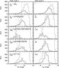 |
Fig. E.1 Number of Ks sources per magnitude in bins of 0.5 mag (dashed line) compared with (full line): the number of Ks sources with also good detections both at J and Ha), northern field; f) southern field; the number of Ks sources with also good detections either at both J and H or at least at H, and in the IRAC 4.5 μm band b), northern field; g) southern field; the number of Ks sources with also good detections in all four IRAC bands c), northern field; h) southern field; the number of Ks sources with also good detections in the first three IRAC bands d), northern field; i) southern field; the number of Ks sources that exhibits an X-ray emission e), northern field; j) southern field. We only took into account sources with photometric uncertainty <0.3 mag in all the considered bands. In addition, the samples plotted in panels c), d), h), i), have been rid of sources with colours indicating PAH contamination as explained in Appendix D. On the upper left corner of each box, a xN tag indicates whether the histograms plotted have been multiplied by a constant N to expand the scale. The vertical dotted lines mark the Ks values at which ~80% of the Ks sources are still retrieved when requiring simultaneous valid detections in other bands. |
Ks values at which 80% of Ks sources are still retrieved when also detected in other bands.
We note that the 80% completeness limit significantly varies from case to case, depending on the colours used and the area of the field. For example, a lot of Ks sources are missed particularly in the northern SofI field when requiring valid detections in all four IRAC bands. This is due to the problems suffered by the two upper wavelength IRAC bands in the regions of diffuse emission outlined in the text. We also note that the JHKs colours mostly tend to filter out embedded stars, young PMS stars and protostars, whereas IRAC colours mostly tend to filter out unreddened stars. Thus, we can hope to obtain a better 80% completeness limit by combining Ks sources for which at least one of the colours from i) to iv) is available. However, as shown in the 6th column of Table E.1, this only happens in the northern SofI field.
The bottom row in Fig. E.1 shows the luminosity function of Ks sources that also exhibit an X-ray emission. Given that not all Ks sources (particularly field stars, unlike T Tauri stars) have detectable X-ray emission, this luminosity function cannot be directly compared with the one of all sources with a valid Ks detection. In the southern field, the luminosity function exhibits a fast increase up to Ks ~ 13. This suggests that all Ks sources emitting X-rays are roughly complete down to that limit. On the other hand, in the northern field the luminosity function is much less steep; if this were mainly due to an increased difficulty in retrieving sources in the northern area of the Ks image, lots of X-ray sources without a NIR counterpart should be detected. Only 5 X-ray sources are actually detected without a NIR counterpart there. So, the flatter X-source Ks luminosity function in the north may arise due to either a decrease in the probability of detecting X-ray emission from embedded cluster members, or a greater Ks magnitude spread of cluster members caused by variable extinction. Therefore, it is difficult to estimate a Ks completeness limit for X-ray emitting sources in this case; it may lie in the range 11–13 mag. However, we note that for strongly variable extinction (as expected when moving from south to north) this would not correspond to a particular mass limit.
Appendix F: Individual NIR sources towards Pismis 24
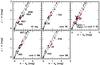 |
Fig. F.1 J − H vs. H − Ks for NIR sources towards the five areas (or subclusters) selected in the SofI field of view. Sources with a JHKs colour excess (and H − Ks< 1) are marked by blue squares, sources with a JH(HKs) [4.5] colour excess (and H − Ks< 1) are marked by red squares, other sources are marked by black squares (small squares for H − Ks ≥ 1). The main sequence locus is also drawn in each diagram, along with reddening (dashed lines with crosses every AV = 10 mag). The sources discussed in the text are labelled, as well. |
The nature of the most massive stars in each subcluster of Pis24 core can be better investigated by considering the corresponding J − H vs. H − Ks (Fig. F.1) and Ks vs. H − Ks diagrams (Fig. F.2). Clearly, all the O-type stars lie towards the south-eastern part of subcluster core C, whereas the other star concentrations are more reminiscent of the small embedded young clusters where typically intermediate-mass stars form. Core SW: it is the only subcluster, apart from core C SE, with a possible earlier-than-B0 star. Our NIR source # 578 is, in fact, bright enough and exhibits a clear JHKs colour excess, suggesting it is a massive young star. H II region: the most massive star towards the Hii region, our NIR source # 998, is a B2 star located on the western part of the bar. The other bright (Ks ~ 10.22) star is located just west of the elephant trunk but is probably a background giant. The star at the tip of the elephant trunk (IRS4 of Felli et al. 1990) is a B0–B4 star with a JHKs colour excess. IRS7 and IRS8 of Felli et al. (1990) also exhibit a JHKs colour excess, but appear to be less massive than IRS4. We found that IRS1 and IRS2 were misplaced by Felli et al. (1990): by comparing their Fig. 4 with our Fig. 2 it can easily be verified that these two sources lie ~15″ further south than the bar (in their Fig. 7), i.e., towards the north-western part of subcluster core C and not in the bar. In addition, Figs. F.2 and F.1 clearly show that they are probably background giants. Core C (NW): the most massive star is a B1–B2 star, our NIR source # 962. It is located near the border between the two parts of subcluster core C, and it could be associated with C SE rather than the C NW. Core NE: it is the only core region hosting an IRAC-retrieved Class I source (with Ks< 13.5), namely our NIR source # 702, which has a characteristic colour excess in the J − H vs. H − Ks diagram (Fig. F.1), as well.
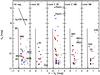 |
Fig. F.2 Ks vs. H − Ks for NIR sources towards the five areas (or subclusters) selected in the SofI field of view. Sources with a JHKs colour excess (and H − Ks< 1) are marked by blue squares, sources with a JH(HKs) [4.5] colour excess (and H − Ks< 1) are marked by red squares, other sources are marked by black squares (small squares for H − Ks ≥ 1). The ZAMS is also drawn in each diagram, whereas an arrow in the first box from left marks an extinction AV = 20 mag. The sources discussed in the text are labelled, as well. |
IRAF is distributed by the National Optical Astronomy Observatory, which is operated by the Associated Universities for Research in Astronomy, Inc., under cooperative agreement with the National Science Foundation.
Acknowledgments
This work is based in part on observations made with the Spitzer Space Telescope, which is operated by the Jet Propulsion Laboratory, California Institute of Technology under a contract with NASA. It is also partially based on observations made with the NASA/ESA Hubble Space Telescope, obtained from the Data Archive at the Space Telescope Science Institute, which is operated by the Association of Universities for Research in Astronomy, Inc., under NASA contract NAS 5-26555. These observations are associated with program # 9091 (P.I. Jeff Hester). This publication makes use of data products from the Two Micron All Sky Survey, which is a joint project of the University of Massachusetts and the Infrared Processing and Analysis Center/California Institute of Technology, funded by the National Aeronautics and Space Administration and the National Science Foundation. The Digitized Sky Survey (DSS) was produced at the Space Telescope Science Institute under US Government grant NAG W–2166. The images of these surveys are based on photographic data obtained using the Oschin Schmidt Telescope on Palomar Mountain and the UK Schmidt Telescope. The plates were processed into the present compressed digital form with the permission of these institutions. F.M. and E.D.C. acknowledge partial funding by the PRIN INAF 2009 grant CRA 1.06.12.10 (“Formation and early evolution of massive star clusters”, P.I. R. Gratton). EDC is also grateful for financial support from PRIN INAF 2011 (“Multiple Populations in Globular Clusters: their role in the Galaxy assembly”, P.I.: E. Carretta).
References
- Allen, C. W. 1976, Astrophysical Quantities, 3rd edn. (London: Athlone press) [Google Scholar]
- Allen, L. E., Calvet, N., D’Alessio, P., et al. 2004, ApJS, 154, 363 [NASA ADS] [CrossRef] [Google Scholar]
- Arthur, S. J., Henney, W. J., Mellema, G., De Colle, F., & Vázquez-Semadeni, E. 2011, MNRAS, 414, 1747 [NASA ADS] [CrossRef] [Google Scholar]
- Baraffe, I., Chabrier, G., & Gallardo, J. 2009, ApJ, 702L, 27 [Google Scholar]
- Beccari, G., Spezzi, L., De Marchi, G., et al. 2010, ApJ, 720, 1108 [NASA ADS] [CrossRef] [Google Scholar]
- Bessell, M. S. 1979, PASP, 91, 589 [NASA ADS] [CrossRef] [Google Scholar]
- Bessell, M. S. 1991, AJ, 101, 662 [NASA ADS] [CrossRef] [Google Scholar]
- Bisbas, T. G., Wünsch, R., Whitworth, A. P., Hubber, D. A., & Walch, S. 2011, ApJ, 736, 142 [Google Scholar]
- Bohigas, J., Tapia, M., Roth, M., & Ruiz, M. T. 2004, AJ, 127, 2826 [NASA ADS] [CrossRef] [Google Scholar]
- Bonnell, I. A., Smith, R. J., Clark, P. C., & Bate, M. R. 2011, MNRAS, 410, 2339 [NASA ADS] [CrossRef] [Google Scholar]
- Cappa, C. E., Barbá, R., Duronea, N. U., et al. 2011, MNRAS, 415, 2844 [NASA ADS] [CrossRef] [Google Scholar]
- Chabrier, G. 2003, PASP, 115, 763 [NASA ADS] [CrossRef] [Google Scholar]
- Chini, R., & Krügel, E. 1983, A&A, 117, 289 [NASA ADS] [Google Scholar]
- Churchwell, E., Watson, D. F., Povich, M. S., et al. 2007, ApJ, 670, 428 [NASA ADS] [CrossRef] [Google Scholar]
- Dale, J. E., & Bonnell, I. A. 2011, MNRAS, 414, 321 [NASA ADS] [CrossRef] [Google Scholar]
- Dale, J. E., Ercolano, B., & Bonnell, I. A. 2012a, MNRAS, 424, 377 [NASA ADS] [CrossRef] [Google Scholar]
- Dale, J. E., Ercolano, B., & Bonnell, I. A. 2012b, MNRAS, 427, 2852 [NASA ADS] [CrossRef] [Google Scholar]
- Damke, G., Barbá, R., Morrell, N. I., et al. 2006, Rev. Mex. Astron. Astrophys., 26, 181 [NASA ADS] [Google Scholar]
- Deharveng, L., & Zavagno, A. 2011, Observations of star formation triggered by Hii regions, in Computational Star Formation, Proc. of the International Astronomical Union, eds. J. Alves, B. G. Elmegreen, J. M. Girart, & V. Trimble, IAU Symp., 270, 239 [Google Scholar]
- Deharveng, L., Zavagno, A., & Caplan, J. 2005, A&A, 433, 565 [NASA ADS] [CrossRef] [EDP Sciences] [Google Scholar]
- De Marchi, G., Panagia, N., Romaniello, M., et al. 2011a, ApJ, 740, 11 [NASA ADS] [CrossRef] [Google Scholar]
- De Marchi, G., Paresce, F., Panagia, N., et al. 2011b, ApJ, 739, 27 [NASA ADS] [CrossRef] [Google Scholar]
- De Marchi, G., Beccari, G., & Panagia, N. 2013, ApJ, 775, 68 [NASA ADS] [CrossRef] [Google Scholar]
- De Silva, G. M., Gibson, B. K., Lattanzio, J., & Asplund, M. 2009, A&A, 500, L25 [NASA ADS] [CrossRef] [EDP Sciences] [MathSciNet] [Google Scholar]
- Dias, W. S., Alessi, B. S., Moitinho, A., & Lépine, J. R. D. 2002, A&A, 389, 871 [NASA ADS] [CrossRef] [EDP Sciences] [Google Scholar]
- Dolphin, A. E. 2000, PASP, 112, 1383 [NASA ADS] [CrossRef] [Google Scholar]
- Dotter, A., Chaboyer, B., Jevremović, D., et al. 2008, ApJS, 178, 89 [NASA ADS] [CrossRef] [Google Scholar]
- Ducati, J. R., Bevilacqua, C. M., Rembold, S. B., & Ribeiro, D. 2001, ApJ, 558, 309 [NASA ADS] [CrossRef] [Google Scholar]
- Fang, M., van Boekel, R., King, R. R., et al. 2012, A&A, 539, A119 [NASA ADS] [CrossRef] [EDP Sciences] [Google Scholar]
- Fazio, G. G., Hora, J. L., Allen, L. E., et al. 2004, ApJS, 154, 10 [NASA ADS] [CrossRef] [Google Scholar]
- Feigelson, E. D., & Montmerle, T. 1999, ARA&A, 37, 363 [NASA ADS] [CrossRef] [Google Scholar]
- Felli, M., Persi, P., Roth, M., et al. 1990, A&A, 232, 477 [NASA ADS] [Google Scholar]
- Fitzpatrick, E. L. 1999, PASP, 111, 63 [NASA ADS] [CrossRef] [Google Scholar]
- Flaccomio, E., Micela, G., & Sciortino, S. 2012, A&A, 548, A85 [NASA ADS] [CrossRef] [EDP Sciences] [Google Scholar]
- Gendelev, L., & Krumholz, M. R. 2012, ApJ, 745, 158 [NASA ADS] [CrossRef] [Google Scholar]
- Getman, K. V., Feigelson, E. D., Kuhn, M. A., et al. 2014, ApJ, 787, 108 [NASA ADS] [CrossRef] [Google Scholar]
- Giannetti, A., Brand, J., Massi, F., Tieftrunk, A., & Beltrán, M. T. 2012, A&A, 538, A41 [NASA ADS] [CrossRef] [EDP Sciences] [Google Scholar]
- Gouliermis, D. A., Schmeja, S., Dolphin, A. E., et al. 2012, ApJ, 748, 64 [NASA ADS] [CrossRef] [Google Scholar]
- Gratton, R. G., Carretta, E., & Bragaglia, A. 2012, A&ARv, 20, 50 [CrossRef] [Google Scholar]
- Gritschneder, M., Burkert, A., Naab, T., & Walch, S. 2010, ApJ, 723, 971 [NASA ADS] [CrossRef] [Google Scholar]
- Groh, J. H., Meynet, G., Ekström, S., & Georgy, C. 2014, A&A, 564, A30 [NASA ADS] [CrossRef] [EDP Sciences] [Google Scholar]
- Guarcello, M. G., Prisinzano, L., Micela, G., et al. 2007, A&A, 462, 245 [NASA ADS] [CrossRef] [EDP Sciences] [Google Scholar]
- Gutermuth, R. A., Megeath, S. T., Myers, P. C., et al. 2009, ApJS, 184, 18 [NASA ADS] [CrossRef] [Google Scholar]
- Gvaramadze, V. V., Kniazev, A. Y., Kroupa, P., & Oh, S. 2011, A&A, 535, A29 [NASA ADS] [CrossRef] [EDP Sciences] [Google Scholar]
- Habets, G. M. H. J., & Heintze, J. R. W. 1981, A&AS, 46, 193 [NASA ADS] [Google Scholar]
- Haisch, K. E., Lada, E. A., & Lada, C. J. 2001, ApJ, 553, L153 [NASA ADS] [CrossRef] [Google Scholar]
- Hartmann, L. 2001, AJ, 121, 1030 [NASA ADS] [CrossRef] [Google Scholar]
- Hillenbrand, L. A. 1997, AJ, 113, 1733 [NASA ADS] [CrossRef] [Google Scholar]
- Holtzman, J. A., Burrows, C. J., Casertano, S., et al. 1995, PASP, 107, 1065 [NASA ADS] [CrossRef] [Google Scholar]
- Indebetouw, R., Mathis, J. S., Babler, B. L., et al. 2005, ApJ, 619, 931 [NASA ADS] [CrossRef] [Google Scholar]
- Jeffries, R. D., Littlefair, S. P., Naylor, T., & Mayne, N. J. 2011, MNRAS, 418, 1948 [NASA ADS] [CrossRef] [Google Scholar]
- Jeffries, R. D., Jackson, R. J., Cottaar, M., et al. 2014, A&A, 563, A94 [NASA ADS] [CrossRef] [EDP Sciences] [Google Scholar]
- Kenyon, S. J., & Hartmann, L. 1995, ApJS, 101, 117 [NASA ADS] [CrossRef] [Google Scholar]
- Koornneef, J. 1983, A&A, 128, 84 [NASA ADS] [Google Scholar]
- Kroupa, P., Tout, C. A., & Gilmore, G. 1993, MNRAS, 262, 545 [NASA ADS] [CrossRef] [Google Scholar]
- Kuhn, M. A., Feigelson, E. D., Getman, K. V., et al. 2014, ApJ, 787, 107 [Google Scholar]
- Lada, C. J., & Lada, E. A. 2003, ARA&A, 41, 57 [NASA ADS] [CrossRef] [Google Scholar]
- Lejeune, T., & Schaerer, D. 2001, A&A, 366, 538 [NASA ADS] [CrossRef] [EDP Sciences] [Google Scholar]
- Lima, E. F., Bica, E., Bonatto, C., & Saito, R. K. 2014, A&A, 568, A16 [NASA ADS] [CrossRef] [EDP Sciences] [Google Scholar]
- Lortet, M.-C., Testor, G., & Niemela, V. 1984, A&A, 140, 24 [NASA ADS] [Google Scholar]
- MaízApellániz, J., Walborn, N. R., Morrell, N. I., Niemela, V. S., & Nelan, E. P. 2007, ApJ, 660, 1480 [NASA ADS] [CrossRef] [Google Scholar]
- Maschberger, T., & Kroupa, P. 2009, MNRAS, 395, 931 [NASA ADS] [CrossRef] [Google Scholar]
- Massey, P., DeGioia-Eastwood, K., & Waterhouse, E. 2001, AJ, 121, 1050 [NASA ADS] [CrossRef] [Google Scholar]
- Massi, F., Brand, J., & Felli, M. 1997, A&A, 320, 972 [NASA ADS] [Google Scholar]
- Massi, F., Testi, L., & Vanzi, L. 2006, A&A, 448, 1007 [NASA ADS] [CrossRef] [EDP Sciences] [Google Scholar]
- Mellema, G., Arthur, S. J., Henney, W. J., Iliev, I. T., & Shapiro, P. R. 2006, ApJ, 647, 397 [NASA ADS] [CrossRef] [Google Scholar]
- Meyer, M. R., Calvet, N., & Hillenbrand, L. A. 1997, AJ, 114, 288 [NASA ADS] [CrossRef] [Google Scholar]
- Moffat, A. F. J., & Vogt, N. 1973, A&AS, 10, 135 [NASA ADS] [Google Scholar]
- Moorwood, A., Cuby, J.-G., & Lidman, C. 1998, The Messenger, 91, 9 [NASA ADS] [Google Scholar]
- Neckel, T. 1978, A&A, 69, 51 [NASA ADS] [Google Scholar]
- Padoan, P., Federrath, C., Chabrier, G., et al. 2014, in Protostars and Planets VI, eds. H. Beuther, R. S. Klessen, C. P. Dullemond, & Th. Henning (University of Arizona Press) [arXiv:1312.5365] [Google Scholar]
- Palla, F., & Stahler, S. W. 1999, ApJ, 525, 772 [NASA ADS] [CrossRef] [Google Scholar]
- Palla, F., & Stahler, S. W. 2000, ApJ, 540, 255 [NASA ADS] [CrossRef] [Google Scholar]
- Parker, R. J., & Meyer, M. R. 2012, MNRAS, 427, 637 [Google Scholar]
- Persson, S. E., Murphy, D. C., Krzeminski, W., Roth, M., & Rieke, M. J. 1998, AJ, 116, 2475 [NASA ADS] [CrossRef] [Google Scholar]
- Preibisch, Th. 2012, RA&A, 12, 1 [Google Scholar]
- Preibisch, Th., & Zinnecker, H. 2002, AJ, 123, 1613 [NASA ADS] [CrossRef] [Google Scholar]
- R core team 2014, R: A Language and Environment for Statistical Computing, R Foundation for Statistical Computing, Vienna, Austria http://www.R-project.org [Google Scholar]
- Ramírez, S. V., Arendt, R. G., Sellgren, K., et al. 2008, ApJS, 175, 147 [NASA ADS] [CrossRef] [Google Scholar]
- Reach, W. T., Megeath, S. T., Cohen, M., et al. 2005, PASP, 117, 978 [NASA ADS] [CrossRef] [Google Scholar]
- Reid, M. J., Menten, K. M., Brunthaler, A., et al. 2014, ApJ, 783, 130 [Google Scholar]
- Rieke, G. H., & Lebofsky, M. J. 1985, ApJ, 288, 618 [NASA ADS] [CrossRef] [Google Scholar]
- Robitaille, T. P., Whitney, B. A., Indebetouw, R., Wood, K., & Denzmore, P. 2006, ApJS, 167, 256 [NASA ADS] [CrossRef] [Google Scholar]
- Robitaille, T. P., Meade, M. R., Babler, B. L., et al. 2008, AJ, 136, 2413 [NASA ADS] [CrossRef] [Google Scholar]
- Russeil, D., Zavagno, A., Adami, C., et al. 2012, A&A, 538, A142 [NASA ADS] [CrossRef] [EDP Sciences] [Google Scholar]
- Scalo, J. 1998, The IMF Revisited: A Case for Variations, in The Stellar Initial Mass Function, Proc. of the 38th Herstmonceux Conf., eds. G. Gilmore, & D. Howell, ASP Conf. Ser., 142, 201 [Google Scholar]
- Siess, L., Dufour, E., & Forestini, M. 2000, A&A, 358, 593 [Google Scholar]
- Spitzer, L. 1978, Diffuse Matter in Space (New York: Interscience) [Google Scholar]
- Stolte, A., Brandner, W., Brandl, B., Zinnecker, H., & Grebel, E. K. 2004, AJ, 128, 765 [NASA ADS] [CrossRef] [Google Scholar]
- Straiz˘ys, V., & Laugalys, V. 2008, Baltic Astron., 17, 253 [NASA ADS] [Google Scholar]
- Tan, J. C., Beltrán, M. T., Caselli, P., et al. 2014, in Protostars and Planets VI, eds. H. Beuther, R. S. Klessen, C. P. Dullemond, & Th. Henning (University of Arizona Press) [arXiv:1402.0919] [Google Scholar]
- Tognelli, E., Prada Moroni, P. G., & Degl’Innocenti, S. 2011, A&A, 533, A109 [NASA ADS] [CrossRef] [EDP Sciences] [Google Scholar]
- Townsley, L. K., Broos, P. S., Garmire, G. P., et al. 2014, ApJS, 213, 1 [NASA ADS] [CrossRef] [Google Scholar]
- Walch, S., Whitworth, A. P., Bisbas, T. G., Wünsch, R., & Hubber, D. A. 2013, MNRAS, 435, 917 [NASA ADS] [CrossRef] [Google Scholar]
- Wand, M. P., & Jones, M. C. 1995, Kernel Smoothing (London: Chapman and Hall) [Google Scholar]
- Wang, J., Townsley, L. K., Feigelson, E. D., et al. 2007, ApJS, 168, 100 [NASA ADS] [CrossRef] [Google Scholar]
- Weidner, C., & Vink, J. S. 2010, A&A, 524, A98 [NASA ADS] [CrossRef] [EDP Sciences] [Google Scholar]
- Westmoquette, M. S., Slavin, J. D., Smith, L. J., & Gallagher, J. S. III 2010, MNRAS, 402, 152 [NASA ADS] [CrossRef] [Google Scholar]
- Whitney, B. A., Wood, K., Bjorkman, J. E., & Cohen, M. 2003, ApJ, 598, 1079 [NASA ADS] [CrossRef] [Google Scholar]
- Whitney, B. A., Indebetouw, R., Bjorkman, J. E., & Wood, K. 2004, ApJ, 617, 1177 [NASA ADS] [CrossRef] [Google Scholar]
- Winston, E., Megeath, S. T., Wolk, S. J., et al. 2007, ApJ, 669, 493 [NASA ADS] [CrossRef] [Google Scholar]
- Zavagno, A., Deharveng, L., Comerón, F., et al. 2006, A&A, 446, 171 [NASA ADS] [CrossRef] [EDP Sciences] [Google Scholar]
- Zinnecker, H., & Yorke, H. W. 2007, ARA&A, 45, 481 [NASA ADS] [CrossRef] [Google Scholar]
All Tables
Estimated [3.6] completeness limits and corresponding stellar masses for given extinction values.
Ks values at which 80% of Ks sources are still retrieved when also detected in other bands.
All Figures
|
Fig. 1 Large scale DSS red image (north up, east left) of the star forming region NGC 6357. The main structures described in the text are marked and labelled. The white stars mark the positions of known star clusters. The length scale is drawn for an assumed distance of 1.7 kpc. |
| In the text | |
|
Fig. 2 Left. Three-colour image (J blue, H green, Ks red) of Pismis 24 and G353.2+0.9, obtained from the reduced SofI frames. Outlined, the HST/WFPC2 field. The border between the two sub-fields and the massive star N78 36 are also indicated. Right. For comparison, three-colour image of the same area obtained by combining the Spitzer/IRAC (short integration) frames at 3.6 μm (blue), 4.5 μm (green) and 8.0 μm (red). A colour version of this figure is available in the on-line edition. |
| In the text | |
|
Fig. 3 Three-colour image (3.6 μm blue, 4.5 μm green, 8.0 μm red) of NGC 6357, obtained from the short-exposure IRAC frames. The large circles mark the locations of the most prominent Hii regions. The clusters Pismis 24 and AH03J1725–34.4 are also labelled. A colour version of this figure is available in the on-line edition. |
| In the text | |
|
Fig. 4 Histogram of the statistics of the surface distribution of IRAC sources detected at least in the two lower-wavelength bands, counted in squares 1′ in size, displaced each other by |
| In the text | |
|
Fig. 5 Left. Contour map of the surface density of IRAC sources, computed as explained in the text. Only sources detected in at least the first two Spitzer/IRAC bands, with photometric errors <0.3 mag, and up to [3.6] = 12.25 are considered. The contours are: 25 stars/arcmin2, 36 stars/arcmin2 (red line), 47 stars/arcmin2, ranging in steps of 3σ (11 stars/arcmin2) from the estimated average surface density (14 stars/arcmin2) of field stars plus 3σ, overlaid on the image at 3.6 μm (grey-scale). Also labelled, the tentatively identified subclusters (A is also known as AH03J1725–34.4). Right. Same as left, but with the positions of identified Class II sources (full blue squares) and Class I sources (open red triangles) superimposed. Other YSO concentrations are enclosed in dashed-line circles. A colour version of this figure is available in the on-line edition. |
| In the text | |
|
Fig. 6 a) SofI J − H vs. H − Ks diagram for the northern field. b) SofI J − H vs. H − Ks diagram for the southern field. c) SofI Ks vs. H − Ks diagram for the northern field. d) SofI Ks vs. H − Ks diagram for the southern field. Only sources with Ks< 16 and photometric errors <0.3 mag have been selected for the colour–colour diagrams, whereas all sources with photometric errors <0.3 mag in H and Ks have been selected for the colour-magnitude diagrams. The datapoint density after smoothing is shown with contours in all panels. The grey triangles mark the sources whose colours have been taken from 2MASS. A few of these sources, associated with Pismis 24, are also indicated, although those labelled G1, G2, and G3 are the candidate background giant stars discussed in the text. The main sequence locus is drawn in all panels with a thick solid line (using the colours from Koornneef 1983, complemented with the absolute magnitudes from Allen 1976 for panels c), d)). Spectral types are labelled next to the ZAMS in panel c). The dashed lines in panels a), b) are reddening paths with crosses every AV = 10 mag (from AV = 0 mag), according to Rieke & Lebofsky (1985), while the thin solid lines are the reddening paths according to the extinction law derived by Straiz˘ys & Laugalys (2008). The dashed line in panels c), d) marks the completeness limit. The arrow in panel c) spans a reddening of AV = 20 mag. Also shown as a full line parallel to the ZAMS in panel c) is the sequence of PMS stars 1 Myr old from the evolutionary tracks of Palla & Stahler (1999), for AV = 10 mag, and masses in the 0.1–6 M⊙ range. A distance of 1.7 kpc is assumed for ZAMS and isochrones. |
| In the text | |
|
Fig. 7 SofI J − H vs. H − Ks diagram for the NIR counterparts of the X-ray sources detected towards Pismis 24. Only sources with photometric errors <0.3 mag have been selected. The thick solid line is the main sequence locus (using the colours from Koornneef 1983). The dotted lines are reddening paths with crosses every AV = 10 mag, following Rieke & Lebofsky (1985). |
| In the text | |
|
Fig. 8 Contour map of the surface density of NIR sources from the SofI data, overlaid with the Ks image of Pismis 24 and G353.2+0.9. Contours range from 240 stars arcmin-2 (the average for field stars plus 2σ, using the values found in the southern field) in steps of 30 stars arcmin-2 (~1σ). Also overlaid: (dashed contour) the surface density of IRAC sources (level 36 stars arcmin-2 of Fig. 5) delineating Pis24 core; (open circles) the location of sources with a NIR excess (see the text for the selection criteria). All data used in figure have Ks< 16 and photometric errors <0.3 mag both in Ks (surface density) and in all JHKs bands (NIR excess). |
| In the text | |
|
Fig. 9 Ks vs. H − Ks for the NIR counterparts of the YSOs towards Pismis 24 identified according to four different indicators, as explained in the text. Open symbols always refer to sources in the northern field, whereas full symbols refer to sources in the southern field. a) YSOs identified on the basis of their IRAC colours (triangles: Class I; squares: Class II); b) YSOs identified on the basis of their combined JH(HKs) [4.5] colours; c) YSOs identified on the basis of their JHKs colours; d) NIR counterparts of X-ray sources. The thick solid vertical line marks the main sequence locus (using absolute magnitudes from Allen 1976 and colours from Koornneef 1983) for a distance modulus of 11.15 mag (d = 1.7 kpc). The arrow in a) shows a reddening of AV = 20 mag according to Rieke & Lebofsky (1985). Spectral types are labelled on the ZAMS. A colour version of this figure is available in the on-line edition. |
| In the text | |
|
Fig. 10 Spatial distribution of the NIR counterparts of the YSOs identified according to four different indicators, as explained in the text, overlaid with the Ks image. Also drawn, a contour of the surface density of Ks sources. Only objects with Ks ≤ 13.5 (unlike Fig. 8, where Ks ≤ 16 has been used) have been selected. a) YSOs identified on the basis of their IRAC colours: red symbols for Class II sources, a large blue triangle marks the only Class I source; b) YSOs identified on the basis of their combined JH(HKs) [4.5] colours; c)JHKs sources exhibiting a colour excess; d) X-ray sources. A colour version of this figure is available in the on-line edition. |
| In the text | |
|
Fig. 11 Dereddened KLFs (see text) for sources in the H − Ks colour interval corresponding to a reddening interval 3.2 <AV< 7.8 (see text) from the mean locus (pseudo-sequence) of young stars. From bottom up: sample selected from the southern field only (pseudo-sequence at 1.7 kpc), from the whole SofI field (pseudo-sequence at 1.7 kpc), and from the whole SofI field (using a pseudo-sequence shifted to a distance of 2.56 kpc). The KLF at the top has been obtained for sources with AV> 7.8 mag picked from the whole field (pseudo-sequence at 1.7 kpc). The two vertical dotted lines mark the completeness limit for the KLF at the top (Ks = 13) and that for the other three KLFs (Ks = 15). |
| In the text | |
|
Fig. 12 Dereddened KLF (see text) for sources in the H − Ks colour interval corresponding to a reddening interval 3.2 <AV< 7.8 (see text) from the mean locus (pseudo-sequence) of young stars (histogram), for Ks counterparts of X-ray sources (full squares), and for sources in the reddening interval 3.2 <AV< 15 (open squares). All are obtained with the pseudo-sequence at 1.7 kpc and from the whole field. Error-bars are derived from Poisson statistics. |
| In the text | |
|
Fig. 13 a)V vs. V − I for stars towards Pismis 24 from HST/WFPC2 images. The full line marks the ZAMS, the dashed lines are isochrones for (from the right) 1, 3, and 10 Myr old PMS stars obtained from the evolutionary tracks of Palla & Stahler (1999). These have been reddened by AV = 5.5 mag and scaled to 1.7 kpc. The loci of 1 and 0.4M⊙ are labelled near the 1 Myr isochrone. Large open triangles are stars without a NIR counterpart, whereas small blue full triangles are stars with X-ray detection. b)Ks vs. H − Ks for the NIR infrared counterparts of the optical stars (red open squares: stars on the left of the optical ZAMS; full squares: stars on the right of the optical ZAMS; blue full triangles: stars on the right of the optical ZAMS also detected in X-ray emission). The full lines are the isochrones for (from the right) 1 and 3 Myr old PMS stars obtained from the evolutionary tracks of Palla & Stahler (1999), same reddening and distance as above. The loci of 1 and 0.4 M⊙ are also labelled and the dashed lines are their reddening paths (for 1 Myr old stars, up to AV = 10 mag, according to Rieke & Lebofsky 1985). c)J − H vs. H − Ks for the NIR infrared counterparts of the optical stars (same symbols as above, but stars on the left of the optical ZAMS are omitted). The full line is the unreddened MS, the dashed lines are reddening paths with crosses every AV = 10 mag, following Rieke & Lebofsky (1985). Also shown as full lines, the reddening paths according to the extinction law derived by Straiz˘ys & Laugalys (2008). The dot-dashed line marks the locus of Classical T Tauri Stars (Meyer et al. 1997). A colour version of this figure is available in the on-line edition. |
| In the text | |
|
Fig. 14 Logarithmic initial mass functions obtained from the dereddened KLFs, each shifted by the amount indicated on the left. The assumed distance moduli, ages, and synthetic tracks (either PMS for low-mass stars, or MS for all stars) are also labelled. The dashed lines show the two-segment fits to the IMFs (for the IMF on the top, the full line is a fit to the whole distribution, which cannot be distinguished in the figure from the fit to the high-mass end only). The vertical dotted lines mark the mass for each distribution at the completeness limit of the corresponding dereddened KLF. |
| In the text | |
|
Fig. B.1 Magnitude–colour diagrams showing the magnitude in the various IRAC bands of the sources from the sample obtained in this work (black dots) as a function of [4.5] – [8.0]. Panels on the same row display, from top to bottom, the measurements for these sources in the 3.6, 4.5, 5.8, and 8.0 μm bands, respectively. In the left column panels, the sources from our sample are overlaid with those from GLIMPSE II (red dots). The green dots in the right column panels are those remaining from our photometry list after removal of sources contaminated by PAH emission. Only objects detected in all four bands with photometric errors <0.3 mag are plotted. |
| In the text | |
|
Fig. B.2 Magnitude–colour diagrams showing the magnitude of all sources from the sample obtained in this work (black dots) only detected in the first three wavelength IRAC bands (i.e., 3.6, 4.5 and 5.8 μm). Panels on the same row display, from top to bottom, the measurements for these sources in the 3.6, 4.5, and 5.8 μm bands, respectively, plotted as a function of [4.5] – [5.8]. In the left column panels, they are overlaid with all sources from GLIMPSE II (red dots) at least detected in the three shorter wavelength bands. The green dots in the right column panels are the sources remaining from our photometry list after removal of those contaminated by PAH emission. Only objects with photometric errors <0.3 mag in the three shorter wavelength bands are plotted. |
| In the text | |
|
Fig. B.3 Magnitude–colour diagrams showing the magnitudes of all sources from the sample obtained in this work (black dots) only detected in the two shorter wavelength IRAC bands (i.e., 3.6 and 4.5μm). Panels on the same row display, from top to bottom, the measurements for these sources in the 3.6 and 4.5μm band, respectively, plotted as a function of [3.6] – [4.5]. On the left column panels, they are overlaid with all sources from GLIMPSE II (red dots) at least detected in the two shorter wavelength bands. Only objects with photometric errors <0.3 mag in the two shorter wavelength bands are plotted. |
| In the text | |
|
Fig. B.4 Number of sources per magnitude bins of 0.5 mag, from our database (black line) and the GLIMPSE sample (red line). The boxes in each row refer to the band indicated on the upper left corner. For the diagrams on the left column we used the sources detected in all four IRAC bands with photometric errors <0.3 mag, whereas for those on the right column we used all sources detected in at least the corresponding band (with photometric errors <0.3 mag in that band). |
| In the text | |
|
Fig. C.1 Number of sources retrieved in the I band vs. [I] in bins of 0.5 mag. The boxes in each row refer to the Spitzer/IRAC band I indicated on the upper left corner of the left-hand box. Upper two rows: in the left column, we compare the I-band sources detected in all IRAC bands with photometric errors <0.3 mag (black line), and the sources detected in at least the first two IRAC bands with photometric errors <0.3 mag (red line); in the right column, we compare all sources detected in at least the first two IRAC bands, with photometric errors either <0.3 mag in both bands (black line), or <0.3 mag in at least the considered band I (blue line). Lower two rows: in the left column, we compare the I-band sources detected in all IRAC bands, with photometric errors either <0.3 mag in all bands (black line), or <0.3 mag in at least the considered band I (red line); in the right column, we compare the I-band sources detected in all IRAC bands, with photometric errors <0.3 mag in at least the considered band I (black line), and the sources detected in at least the considered band I with photometric errors <0.3 mag (blue line). |
| In the text | |
|
Fig. D.1 Magnitude vs. [5.8] – [8.0] in the 3.6 μm (left) and 8.0 μm (right) bands for all sources in our sample with detections in all four bands and photometric errors <0.3 mag (black dots). Overlaid (green dots), all remaining sources after removal of the various contaminants as explained in the text. |
| In the text | |
|
Fig. D.2 [3.6] – [4.5] vs. [5.8] – [8.0] (left) and [4.5] – [5.8] vs. [5.8] – [8.0] (right) for all sources in our sample detected in all four bands with photometric errors <0.3 mag (black dots). Overlaid (green dots), all remaining sources after removal of the various contaminants as explained in the text. |
| In the text | |
|
Fig. D.3 [8.0] vs. [5.8] – [8.0] for all sources in our sample only detected at 5.8 and 8.0 μm. |
| In the text | |
|
Fig. D.4 IRAC colour–colour diagrams. Top panel, [3.6] – [4.5] vs. [5.8] – [8.0] for sources detected in all four bands and with photometric errors <0.3 mag. Bottom panel, [3.6] – [4.5] vs. [4.5] – [5.8] for the same sources as above, plus those only detected in the three shorter wavelength bands (with photometric errors <0.3 mag). The two samples have been cleaned of contaminants as explained in the text. Following the prescriptions of Gutermuth et al. (2009) for their identification, Class I sources are in red and Class II sources in blue. Stars are marked as black dots. A reddening corresponding to AV = 20 mag (according to Indebetouw et al. 2005) is marked by an arrow. In the top panel, the regions occupied by Stage I and Stage II sources (Robitaille et al. 2006) are also outlined. |
| In the text | |
|
Fig. E.1 Number of Ks sources per magnitude in bins of 0.5 mag (dashed line) compared with (full line): the number of Ks sources with also good detections both at J and Ha), northern field; f) southern field; the number of Ks sources with also good detections either at both J and H or at least at H, and in the IRAC 4.5 μm band b), northern field; g) southern field; the number of Ks sources with also good detections in all four IRAC bands c), northern field; h) southern field; the number of Ks sources with also good detections in the first three IRAC bands d), northern field; i) southern field; the number of Ks sources that exhibits an X-ray emission e), northern field; j) southern field. We only took into account sources with photometric uncertainty <0.3 mag in all the considered bands. In addition, the samples plotted in panels c), d), h), i), have been rid of sources with colours indicating PAH contamination as explained in Appendix D. On the upper left corner of each box, a xN tag indicates whether the histograms plotted have been multiplied by a constant N to expand the scale. The vertical dotted lines mark the Ks values at which ~80% of the Ks sources are still retrieved when requiring simultaneous valid detections in other bands. |
| In the text | |
|
Fig. F.1 J − H vs. H − Ks for NIR sources towards the five areas (or subclusters) selected in the SofI field of view. Sources with a JHKs colour excess (and H − Ks< 1) are marked by blue squares, sources with a JH(HKs) [4.5] colour excess (and H − Ks< 1) are marked by red squares, other sources are marked by black squares (small squares for H − Ks ≥ 1). The main sequence locus is also drawn in each diagram, along with reddening (dashed lines with crosses every AV = 10 mag). The sources discussed in the text are labelled, as well. |
| In the text | |
|
Fig. F.2 Ks vs. H − Ks for NIR sources towards the five areas (or subclusters) selected in the SofI field of view. Sources with a JHKs colour excess (and H − Ks< 1) are marked by blue squares, sources with a JH(HKs) [4.5] colour excess (and H − Ks< 1) are marked by red squares, other sources are marked by black squares (small squares for H − Ks ≥ 1). The ZAMS is also drawn in each diagram, whereas an arrow in the first box from left marks an extinction AV = 20 mag. The sources discussed in the text are labelled, as well. |
| In the text | |
Current usage metrics show cumulative count of Article Views (full-text article views including HTML views, PDF and ePub downloads, according to the available data) and Abstracts Views on Vision4Press platform.
Data correspond to usage on the plateform after 2015. The current usage metrics is available 48-96 hours after online publication and is updated daily on week days.
Initial download of the metrics may take a while.