| Issue |
A&A
Volume 561, January 2014
|
|
|---|---|---|
| Article Number | A128 | |
| Number of page(s) | 19 | |
| Section | Numerical methods and codes | |
| DOI | https://doi.org/10.1051/0004-6361/201321102 | |
| Published online | 22 January 2014 | |
A new method to improve photometric redshift reconstruction
Applications to the Large Synoptic Survey Telescope
1 Laboratoire de Physique Subatomique et de Cosmologie, UJF/INP/CNRS/IN2P3, 53 avenue des Martyrs, 38026 Grenoble Cedex, France
2 Laboratoire de l’Accélérateur Linéaire, Univ. Paris Sud/CNRS/IN2P3, Bât. 200, 91898 Orsay Cedex, France
3 Physics Department, University of Arizona, 1118 East 4th Street, Tucson, AZ 85721, USA
e-mail: abate@email.arizona.edu
Received: 14 January 2013
Accepted: 21 September 2013
Context. In the next decade, the Large Synoptic Survey Telescope (LSST) will become a major facility for the astronomical community. However, accurately determining the redshifts of the observed galaxies without using spectroscopy is a major challenge.
Aims. Reconstruction of the redshifts with high resolution and well-understood uncertainties is mandatory for many science goals, including the study of baryonic acoustic oscillations (BAO). We investigate different approaches to establish the accuracy that can be reached by the LSST six-band photometry.
Methods. We construct a realistic mock galaxy catalog, based on the Great Observatories Origins Deep Survey (GOODS) luminosity function, by simulating the expected apparent magnitude distribution for the LSST. To reconstruct the photometric redshifts (photo-z’s), we consider a template-fitting method and a neural network method. The photo-z reconstruction from both of these techniques is tested on real Canada-France-Hawaii Telescope Legacy Survey (CFHTLS) data and also on simulated catalogs. We describe a new method to improve photometric redshift reconstruction that efficiently removes catastrophic outliers via a likelihood ratio statistical test. This test uses the posterior probability functions of the fit parameters and the colors.
Results. We show that the photometric redshift accuracy will meet the stringent LSST requirements up to redshift ~2.5 after a selection that is based on the likelihood ratio test or on the apparent magnitude for galaxies with signal-to-noise ratio S/N > 5 in at least 5 bands. The former selection has the advantage of retaining roughly 35% more galaxies for a similar photo-z performance compared to the latter. Photo-z reconstruction using a neural network algorithm is also described. In addition, we utilize the CFHTLS spectro-photometric catalog to outline the possibility of combining the neural network and template-fitting methods.
Conclusions. We demonstrate that the photometric redshifts will be accurately estimated with the LSST if a Bayesian prior probability and a calibration sample are used.
Key words: cosmology: observations / techniques: photometric / surveys / galaxies: photometry / galaxies: distances and redshifts / galaxies: luminosity function, mass function
© ESO, 2014
1. Introduction
The Large Synoptic Survey Telescope (LSST) has an optimal design for investigating the mysterious dark energy. With its large field of view and high transmission bandpasses, the LSST will be able to observe a tremendous amount of galaxies, out to high redshift, over the visible sky from Cerro Pachón over ten years. This will lead to an unprecedented study of dark energy, among other science programs such as the study of the Milky Way and our Solar System (LSST Science Collaboration 2009).
One of the main systematic uncertainties in the cosmological analysis will be tightly related to errors in the photometric redshift (photo-z) estimation. Estimating the redshift from the photometry alone (Baum 1962) is indeed much less reliable than using spectroscopy, although it does allow measurements to be obtained for vastly more galaxies, especially for those that are very faint and distant. Photo-z estimates are mainly sensitive to characteristic changes in the galaxy’s spectral energy distribution (SED), such as the Lyman and the Balmer breaks at 100 nm and 400 nm, respectively. Incorrect identifications between these two main features greatly impact the photometric redshifts and are an example of how catastrophic photo-z outliers can arise. Mischaracterizing the proportion of these outliers will strongly impact the level of systematic uncertainties.
There are basically two different techniques to compute the photo-z. On the one hand, template-fitting methods (e.g. Puschell et al. 1982; Bolzonella et al. 2000) fit a model galaxy SED to the photometric data and aim to identify the spectral type, the redshift, and possibly other characteristics of the galaxy. It has been proven that using spectroscopic information in the template-fitting procedure, by introducing a Bayesian prior probability (Benítez 2000) or by modifying the SED template (Budavári et al. 2000; Ilbert et al. 2006) for example, improves the photo-z quality. This highlights the necessity to have access to at least some spectroscopic data.
On the other hand, empirical methods extract information from a spectroscopic training sample and are therefore generally limited to the spectroscopic redshift range of the sample itself. Among these, the empirical color-redshift relation (Connolly et al. 1995; Sheldon et al. 2012) and neural networks (Vanzella et al. 2004; Collister & Lahav 2004) are commonly used.
In this paper, we address the issue of estimating the photo-z quality with a survey similar to the LSST, and in particular, we introduce a new method, the likelihood ratio statistical test, that aims to remove most of the galaxies with catastrophic redshift determination (hereafter called outliers). We utilize a galaxy photometric catalog, which is simulated for a study of the uncertainty that is expected from the LSST determination of the dark energy equation of state parameter using baryon acoustic oscillations (BAO). The related results will be presented in a companion paper by Abate et al. (in prep.).
Based on a Bayesian χ2 template-fitting method, our photo-z reconstruction algorithm gives access to the posterior probability density functions (pdf) of the fit parameters. Using a training sample, the likelihood ratio test, which is based on the characteristics of the posterior pdf and the colors, is calibrated and then applied to each galaxy in the photometric sample. The technique is tested on a spectro-photometric catalog from the T0005 data release of CFHTLS1 that is matched with spectroscopic catalogs from VIMOS-VLT Deep Survey (VVDS; Le Fevre et al. 2005; Garilli et al. 2008), DEEP2 (Newman et al. 2013) and zCOSMOS (Lilly et al. 2007). We also outline the possibility to discard outlier galaxies by using photometric redshifts estimated from both the template-fitting method and a neural network.
Finally, we illustrate the modification to the systematic and statistical uncertainties on the photo-z when the redshift distribution of the training sample is biased compared to the actual redshift distribution of the photometric catalog to be analyzed.
The paper is organized as follows. The LSST is presented in Sect. 2.1 and followed by our simulation method in Sect. 2.2. In the latter, the simulation steps employed and the physical ingredients required to produce the mock galaxy catalogs are described. In Sect. 2.3, the mock galaxy catalogs for Great Observatories Origins Deep Survey (GOODS), CFHTLS, and LSST are presented and validated against data for the former two surveys. Our template-fitting method and the likelihood ratio test are described in Sect. 3. The performance of our photo-z template-fitting method is shown in Sect. 4. In Sect. 5, the photo-z neural network technique and its performance in conjunction with our template-fitting method is investigated. Finally, we give a brief discussion of the current limitations of our simulations in Sect. 6 and conclude in Sect. 7.
Throughout the paper, we assume a flat cosmological ΛCDM model with the following parameter values: Ωm = 0.3, ΩΛ = 0.7, Ωk = 0, and H0 = 70 km s-1/Mpc. Unless otherwise noted, all magnitudes given are in the AB magnitude system.
2. Simulation description and verification
2.1. The Large Synoptic Survey Telescope
The LSST is a ground-based optical telescope survey designed in part to study the nature of dark energy. It will likely be one of the fastest and widest telescopes of the coming decades. The same data sample will be used to study the four major probes of dark energy cosmology: type 1a supernovae, weak gravitational lensing, galaxy cluster counts, and baryon acoustic oscillations.
The LSST will be a large aperture 8.4 m diameter telescope with a 3200 Megapixel camera. It will provide unprecedented photometric accuracy with six broadband filters (u,g,r,i,z,y). Figure 2 shows the LSST transmission curves, including the transmissions of the filters, the expected CCD quantum efficiency, and the optics throughput. The field of view will be 9.6 deg2 and the survey should cover 30 000 deg2 of sky visible from Cerro Pachón.
The LSST will perform two back-to-back exposures of 2 × 15 s with a readout time of 2 × 2 s. The number of visits and the (5σ) limiting apparent magnitude in each band for the point sources for one year and ten years of the running survey are listed in Table 1. With such deep observations, photometric redshifts will necessarily be computed in an essentially unexplored redshift range.
The photo-z requirements, as published in the LSST Science Book (LSST Science Collaboration 2009), are given in Table 2.
The final specifications of the LSST are subject to change; see Ivezic et al. (2008) for the latest numbers.
Number of visits and 5σ limiting apparent magnitudes (point sources), for one year and ten years of LSST operation (Ivezic et al. 2008; Petry et al. 2012).
LSST photo-z requirements for the high signal-to-noise “gold sample” subset, which is defined as having i < 25.3.
2.2. Simulation of galaxy catalogs
The simulation method we employ is to draw basic galaxy attributes: we consider redshift, luminosity, and type from observed distributions, assign each galaxy a SED and a reddening based on those attributes, and then calculate the observed magnitudes expected for the survey in question. For similar efforts, see the following work: Dahlen et al. (2008) for a SNAP2-like mission, Jouvel et al. (2009) for JDEM3/Euclid-like missions, Benítez et al. (2009) for the PAU4 survey.
2.2.1. Simulating galaxy distributions
To simulate the galaxy catalog, we first compute the total number of galaxies N within our survey volume between absolute magnitudes M1 and M2. Then we assign redshifts and galaxy types for each of these N galaxies.
If φ is the sum of luminosity functions over the early, late and starburst galaxy types (see Sect. 2.2.3 for more details), then the number of galaxies Ng is given by 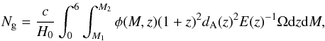 (1)where M is the absolute magnitude in some band, dA(z) is the angular diameter distance, the function
 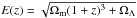 , and Ω (no subscript) is the solid angle of the simulated survey. The redshift range is chosen so as not to miss objects that may be observable by the survey. We chose to use luminosity functions observed from the GOODS survey in the B-band. The exact choice of M1 and M2 is not critical, since: (i) at the bright limit, the luminosity function goes quickly to zero; therefore the integral does not depend on M1 as long as it is less than − 24. (ii) As long as M2 is chosen to be fainter than the maximum absolute magnitude observable by the survey, then all galaxies that are possible to observe are included in the integral. We calculated this to be M2 = −13. The redshift zs of each simulated galaxy is drawn from the cumulative density function:
 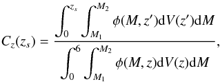 (2)where dV is the comoving volume element. Once the redshift of the galaxy, denoted by zs, is assigned, the absolute magnitude M is drawn from the following cumulative density function
 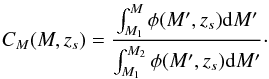 (3)Finally, a broad galaxy type is assigned from the observed distribution of each type at redshift zs and absolute magnitude M. This distribution is constructed from the type-dependent luminosity functions. Therefore, each galaxy is designated a broad type value of either early, late or starburst. An SED from the library is then selected for each galaxy, according to the simulation procedure described in Sect. 2.2.4.
2.2.2. Simulating the photometric data
The simulated apparent magnitude mX,s5 in any LSST band X with transmission X(λ) for a galaxy of SED type Ts6, redshift zs, color excess E(B − V)s, and absolute magnitude MY,s is generated as follows:  (4)where μ(zs) is the distance modulus and KXY(zs,Ts,E(B − V)s) is the K-correction, defined as described in Hogg et al. (2002) for spectral type Ts, with flux observed in observation-frame band X and MY,s in rest-frame band Y. Then, the magnitude is converted into the corresponding simulated flux FX,s value. The simulated observed flux FX,obs is drawn from a Gaussian with a mean FX,s and standard deviation σ(FX,s). This is correct as long as the flux is large enough to be well distributed with a Gaussian distribution. The uncertainty σX(mX,s) on true magnitude in band X is given by Eq. (7) in Sect. 2.2.7.
Note that the apparent magnitude uncertainty σX(mX,s) depends on the number of visits NX,vis. We have performed the simulation for two sets of values of NX,vis that correspond to one and ten years of observations with the LSST, according to the NX,vis given in Table 1.
Throughout the paper, the quantity zs refers to the simulated or true value of the redshift. Here we also assume that a spectroscopic redshift obtained for one of the simulated galaxies has a value equal to zs. Therefore, the value zs can be also considered to be the galaxy’s spectroscopic redshift with negligible error.
2.2.3. Luminosity function
The luminosity function probabilistically describes the expected number of galaxies per unit volume and per absolute magnitude. If the luminosity functions are redshift- and type-dependent, then they give the relative amount of galaxies for each galaxy type at a given redshift.
We use luminosity functions measured from the GOODS survey (Dahlen et al. 2005). The luminosity functions here are modeled by a parametric Schechter function that takes the form:  where M is the absolute magnitude in the B-band of GOODS Wide Field Imager (WFI), and M⋆, φ⋆, and α are the parameters defining the function. Their values can be obtained from Dahlen et al. (2005).
2.2.4. Spectral energy distribution library
We built a SED library composed of 51 SEDs. They were created by interpolating between six template SEDs, as described here:
-
the early-type El, the late-types Sbc, Scd and the starburst-type Imfrom Coleman et al. (1980);
-
the starburst-types SB3 and SB2 from Kinney et al. (1996).
These six original SEDs were linearly extrapolated into the UV by using the GISSEL7 synthetic models from Bruzual & Charlot (2003). The interpolated spectra of the 51 types are displayed in Fig. 1. In the following, we denote by Ts the true spectral type (SED) of the galaxy.
Each galaxy is assigned a SED from this library using a flat probability distribution based on their broad type value, originally assigned as either early, late or starburst (see Sect. 2.2.1). This way of generating the spectra may not be as optimal as using more realistic synthetic spectra, but it has heuristic advantages. For example, there is an easy way to relate the galaxy type of the luminosity function to a SED type, and additionally it is much faster, in terms of computing time, to produce a large amount of galaxy spectra at different evolutionary stages. We are aware, however, that this linear interpolation may bias photometric redshifts that are estimated using a template-fitting method, because real galaxies are probably not evenly distributed across spectrum space. Therefore, this feature may allow the neural network method to be more effective in estimating the redshift.
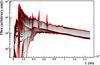 |
Fig. 1 SED templates are linearly interpolated from the original six templates from Coleman et al. (1980) and Kinney et al. (1996). The original templates are drawn in red. |
2.2.5. Attenuation by dust and intergalactic medium
The reddening caused by dust within the target galaxy is quantified in our simulation by the color excess term E(B − V). With this term, the Cardelli law (Cardelli et al. 1989) is used for the galaxies closest to the El, Sbc, and Scd spectral types, whereas the Calzetti law is used for the galaxies closest to the Im, SB3, and SB2 spectral types. The color excess E(B − V) is drawn from a uniform distribution between 0 to 0.3 for all galaxies, except for galaxies closest to the El type. Indeed, elliptical galaxies are composed of old stars and contain little or no dust; therefore, E(B − V) is drawn only between 0 to 0.1 for these galaxies.
Another process to be considered is the absorption due to the intergalactic medium (IGM). It is caused by clumps of neutral hydrogen along the line of sight and is well-modeled by the Madau law (Madau 1995). As the absorption occurs at a fixed wavelength in the hydrogen reference frame, it is redshift-dependent in the observer frame. Strong features in the optical part of the SEDs are induced by the IGM at redshifts above about z ~ 2.8 in the LSST filter set, when the Lyman-α forest has shifted into the LSST band passes. Here we assume this absorption to be constant with the line of sight to the galaxy. An investigation of the effect of the stochasticity of the IGM will be the subject of future work.
2.2.6. Filters
The six LSST bandpasses displayed in Fig. 2 include the quantum efficiency of the CCD, the filter transmission, and the telescope optical throughput. The CFHTLS filter set8 is also displayed in the same figure. We expect to be able to obtain good photo-z estimates up to redshifts of about 1.2 for CFHTLS and 1.4 for LSST when the 4000 Å break is redshifted out of the filter sets. At redshifts above 2.5, the precision should improve dramatically when the Lyman break begins to redshift into the u-band.
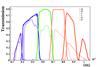 |
Fig. 2 LSST transmission curves shown by the solid lines and CFHTLS transmissions shown by the dashed lines. The transmission includes the transmission of the filter itself, the expected CCD quantum efficiency, and the telescope optical throughput. |
2.2.7. Apparent magnitude uncertainties for the LSST
The apparent magnitude uncertainties for the LSST are computed following the semi-analytical expression from the LSST Science Book (LSST Science Collaboration 2009). This expression has been evaluated from the LSST exposure time calculator, which considers the instrumental throughput, the atmospheric transmission, and the airmass among other physical parameters.
The total uncertainty on the apparent magnitude includes a systematic uncertainty that comes from the calibration, such that the photometric error in band X is  (7)where σrand,X is the random error on the magnitude and σsys,X is taken to be equal to 0.005 and is the photometric systematic uncertainty of the LSST for a point source. We have adopted this simple formula defined for point sources and have used it for extended sources. A more realistic computation of this uncertainty for extended sources will be completed in future work (see also Sect. 6).
2.2.8. Apparent magnitude uncertainties for CFHTLS and the GOODS survey
An analytical expression similar to the one given by Eq. (7) does not exist for the CFHTLS and the GOODS data. The apparent magnitude uncertainties are estimated with algorithms and analysis techniques specific to these surveys and the relations described in the previous Sect. does not apply.
In the following, where simulations of photometric galaxy catalogs of both of these surveys are carried out, the simulated uncertainties on the apparent magnitudes are estimated directly from the survey data themselves. In this way, one can obtain the probability distribution of having σX given mX. This allows the assignment of σX by randomly drawing the value, according to this probability density function, given the value of mX.
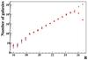 |
Fig. 3 Histograms of the apparent magnitude in the R band comparing the GOODS simulated data (black points with error bars) to the actual GOODS data (red stars). We note that there may be a systematic shift in all data points in the x-axis direction up to R ≲ 0.05 mag due to differences between the simulation and data filter zero points. |
2.3. Method validation
2.3.1. GOODS
To validate the simulation scheme, we have performed a simulation of the GOODS WFI data9 and compared our results to the real photometric catalog used for the computation of the B-band luminosity functions reported in Dahlen et al. (2005).
The simulated photometric catalog corresponds to an effective solid angle of 1100 arcmin2, which is equal to the area covered by the actual data catalog. The simulated redshift and absolute magnitude ranges are respectively [0,6] and [−24, −13]. The apparent magnitudes are computed for the WFI B-band and R-band. The apparent magnitude uncertainty is now given by the distribution of σX given mX computed from the real data (see 2.2.8). If mX,s is the simulated apparent magnitude in any X-band, the uncertainty is randomly drawn from the distribution Prob(σX|mX,s) found from the data. The observed apparent magnitude and its uncertainty are then simulated as detailed in Sect. 2.2.2.
Figure 3 shows the very good agreement of the galaxy number counts in the R-band between the simulation and the real data, except for the very faint galaxies at R ≥ 25, where the selection effect in the real data becomes important. The agreement is also very good for the B-band (not shown here). As displayed in Fig. 4, the distributions of colors from our GOODS simulation (black lines) reasonably agree with the ones from the real data (red lines) for bright and faint galaxies. At bright magnitudes, the fitted luminosity function seems to predict a larger fraction of elliptical galaxies than the data. This feature probably comes from the SED templates and their linear interpolation. We have chosen to interpolate linearly between the SED templates with an equal number of steps between each template. With real galaxies, it could easily be that this is not the case; perhaps, for example, the distribution of the galaxy’s SEDs is not uniform between the El and the Sbc galaxy type. Instead it could be more probable for an intermediate SED to be more similar to the Sbc. This reasoning could explain our excess. Since El galaxies exist only in significant numbers at low redshift and photo-z’s are well estimated at low redshift, this excess should not have any impact on our conclusions. In any case, the overall shape of the distributions indicates that our simulated photometric catalog represents reality. This is expected because the luminosity functions were computed from the real data sample used for the comparison to the simulation.
Number of galaxies that are both observed photometrically with the CFHTLS survey and spectroscopically.
2.3.2. CFHTLS
The different photo-z reconstruction methods were tested on real data, namely on galaxies observed both photometrically (from CFHTLS T0005) and spectroscopically (from either VVDS, DEEP2 or zCOSMOS surveys). We have followed the procedure described in detail by Coupon et al. (2009).
The CFHTLS T0005 public release contains a photometric catalog of objects observed in five bands (u,g,r,i,z) from the D1, D2, D3, W1, W3, and W4 fields. Among these, some galaxies are also spectroscopically observed by the VVDS, DEEP2 Redshift Survey, and zCOSMOS surveys. The numbers of galaxies in the CFHTLS fields that were matched to spectroscopic observations are listed in Table 3. To perform the matching, the smallest angle between each galaxy in the CFHTLS catalog and a galaxy from the spectroscopic catalogs was computed. Only galaxies for which the angle is less than 0.7 arcsec (the order of the point spread function) are grouped into the spectro-photometric catalog. Since we also required the galaxies to be detected in all CFHTLS bands, the spectro-photometric sample is not as large as direct matching between the catalogs would produce.
The spectroscopic redshift distribution of the spectro-photometric catalog is shown in Fig. 5. A simulation of the CFHTLS data was also performed. This was to enable us to evaluate whether the statistical test described in Sect. 3.2 could be calibrated with a simulation and then applied to real data, for which the spectroscopic redshifts of galaxies are not known. This procedure would be useful if no spectroscopic sample is available to calibrate the prior probabilities or the likelihood ratio statistical test presented in Sect. 3.2. The same argument stands for the neural network analysis described in Sect. 5, which could also benefit from a simulated training sample.
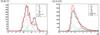 |
Fig. 4 Histograms of the B − R term for different apparent magnitude ranges. Left-hand panel (20 < R < 22) corresponds to the bright galaxies and right-hand panel (24 < R < 25.5) corresponds to the very faint galaxies. The solid black lines correspond to the simulation and the solid red lines correspond to the GOODS data. The dotted colored lines correspond to the main spectral types in the simulation. |
Because the selection function of the spectro-photometric catalog is not only based on the detection threshold, the redshift and color distributions of the simulation and real data cannot be rigorously compared. The photometric selection criteria is not homogeneous over this data sample due to the differing selection of VVDS, DEEP2, and zCOSMOS, and, therefore, does not match the simulation. However, we can qualitatively compare the color distribution domains of galaxies from the CFHTLS catalog with the ones obtained from the simulations.
Figure 6 shows two color–color distributions, (u − g) vs. (g − r) and (g − r) vs. (r − i), for the CFHTLS data, on which we have superimposed (red) the distribution obtained from calculating the expected magnitudes, given the fitted values of photo-z, galaxy template, and reddening, which are obtained by running the photo-z algorithm on the data (as described in Sect. 3). It can be seen that there is a satisfactory agreement between the domains covered by the data and our simulations, indicating that our templates represent the galaxies well. We have also checked the compatibility of color variations with the redshift for data and simulations, especially for early and late type galaxies.
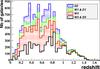 |
Fig. 5 Redshift distribution of the spectroscopic sample for the different CFHTLS fields. The histograms are stacked. |
2.3.3. LSST forecasts
The simulated LSST sample considered here is the same as the one used in the companion paper Abate et al. (in prep.). It is generated with a solid angle of 7850 deg2 and a redshift range of [0.1,6]. This upper redshift limit is large enough to include all observable galaxies. The total number of galaxies is ~8 × 10⁹. For the purpose of this paper, namely the reconstruction of photometric redshifts, such a large number of galaxies is not necessary. Therefore, the following analysis is done with a smaller subsample of galaxies, as seen Sect. 4.2.
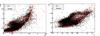 |
Fig. 6 Color–color plots showing the relation between CFHTLS data (black dots) and the distribution expected from our SED template set (red dots). |
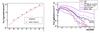 |
Fig. 7 Left-hand side: cumulative distribution of the apparent magnitude in the i band for the LSST simulation compared to the Sloan Digital Sky Survey (SDSS) measurement from the Stripe 82 region (cf. Abazajian et al. 2009). The statistical error bars from the data are smaller than the dots size. Right-hand side: redshift distribution of galaxies for the LSST: i < 24, i < 25 with σi < 0.2 (solid red, solid black curves respectively); i < 27 with S ! N > 5 in at least the i band for one and ten years of observations (dotted and solid magenta respectively); S ! N > 5 in all bands for one and ten years of observations (dotted and solid blue respectively). |
The expected cumulative number counts per unit of solid angle and per i band apparent magnitude for the LSST is shown on the left-hand side of Fig. 7, and is compared to the SDSS measurements made on the Stripe 82 region (cf. Abazajian et al. 2009). The LSST galaxy count is generally below that of SDSS with a more pronounced effect at high and low end magnitudes (m ~ 26 and m ~ 20). The discrepancy (Fig. 7, left-hand side) might be due to a systematic zero point magnitude error in the simulation due to an imperfect filter model, excessive absorption (extinction) in the simulation, or uncorrected differences between the selection of SDSS galaxies and GOODS galaxies.
The expected number of galaxies per unit of solid angle and per redshift is shown on the right-hand side of Fig. 7 for different cuts: i magnitude cuts of i < 24, i < 25, and i < 27 with σX < 0.2 for all X bands for both one (dotted lines) and ten years (solid lines) of observations. The LSST gold sample is defined as all galaxies with i < 25.3, so that it will contain around 4 billion galaxies that have up to a redshift of 3 and is expected to produce high quality photometric redshifts.
The number of galaxies with S / N > 5 in all six bands at ten years is fairly small because these constraints are strong for the low acceptance u and y bands. Low S/N in the u-band is expected from both its shallower depth and dropout galaxies at higher redshift, where hydrogen absorption removes all flux blueward of the Lyman break, and non-detections above z > 3 are expected. The low S/N in the y-band is expected just from its shallower depth.
3. Enhanced template-fitting method
3.1. Maximum of the posterior probability density function
In this section, our template-fitting method for estimating photometric redshifts is presented. The algorithm follows the approach developed by Ilbert et al. (2006), Bolzonella et al. (2000), or Benítez (2000).
Basically, the template-fitting method consists in finding the photo-zzp, the SED template Tp, the color excess E(B − V)p10, and the SED normalization N that give the fluxes in each band that best fit to the observed values. Following Benítez (2000), the normalization parameter is marginalized over, so that the parameters of interest are given by the minimum of a χ2 statistic, whose expression is given later in this section.
A Bayesian prior probability can be used to improve the photometric redshift reconstruction. It is defined as the probability of having a galaxy of redshift z and type T, given its apparent magnitude. It was introduced by Benítez (2000). Bayes’ theorem indicates that this probability can be expressed as the product of the probability of having a galaxy of type T given the apparent magnitude i, P(T|i) times the probability of having a galaxy of redshift z, given the type and the apparent magnitude, P(z|T,i). In other words,  (8)The two terms are well described by the functions,
 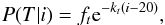 (9)and
 ![\begin{eqnarray} \label{Eq:PzTI} P(z|T,i) & \propto& z^{\alpha} \exp\left[ -\left(\frac{z}{z_m }\right)^\alpha \right],\nonumber \\ z_m &=& z_0+k_m(i-16) + p_m(i-16)^{\beta}. \end{eqnarray}](/articles/aa/full_html/2014/01/aa21102-13/aa21102-13-eq117.png) (10)Here, T represents the spectral family (broad type) instead of the spectral type (the exact SED). That is, galaxies with a spectral type that is lower than 5 belong to the early-type, those with spectral type between 6 and 25 belong to the late-type and the rest belong to the starburst-type. This parametrization follows a general model for galaxy number counts with redshift and is improved to account for higher redshifts in CFHTLS by the addition of the pm and β parameters, as compared to Eqs. (22)–(24) in Benítez (2000). The parameters of P(T|i) and P(z|T,i) are found from fitting Eqs. (9) and (10) to the simulated magnitude-redshift distributions for both the LSST and CFHTLS surveys. The value of the parameters in Eqs. (9) and (10) are given by Table 4. The fitted pm parameter for the LSST is compatible with zero. While it is meaningful for CFHTLS (see Table 4), it is therefore set to zero when representing the prior probability for the LSST simulations. There is no value for the parameters ft and kt for Starburst galaxies, whose probability distribution is set by the condition that the sum of probabilities over all galaxy types must be equal to 1.
(10)Here, T represents the spectral family (broad type) instead of the spectral type (the exact SED). That is, galaxies with a spectral type that is lower than 5 belong to the early-type, those with spectral type between 6 and 25 belong to the late-type and the rest belong to the starburst-type. This parametrization follows a general model for galaxy number counts with redshift and is improved to account for higher redshifts in CFHTLS by the addition of the pm and β parameters, as compared to Eqs. (22)–(24) in Benítez (2000). The parameters of P(T|i) and P(z|T,i) are found from fitting Eqs. (9) and (10) to the simulated magnitude-redshift distributions for both the LSST and CFHTLS surveys. The value of the parameters in Eqs. (9) and (10) are given by Table 4. The fitted pm parameter for the LSST is compatible with zero. While it is meaningful for CFHTLS (see Table 4), it is therefore set to zero when representing the prior probability for the LSST simulations. There is no value for the parameters ft and kt for Starburst galaxies, whose probability distribution is set by the condition that the sum of probabilities over all galaxy types must be equal to 1.
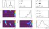 |
Fig. 8 Example of photometric computation for a simulated galaxy observed with the LSST in six bands at 5σ for ten years of observation. The 2D distributions correspond to the posterior probability density functions marginalized over the remaining parameter, and the 1D distributions correspond to the posterior probability density functions marginalized over the two remaining parameters. The top middle panel corresponds to the value of the input parameters. On the top right-hand panel, the index grid denotes the parameters that maximize the 3D posterior probability density function on the grid, and on the middle right-hand panel, the index marg denotes the parameters that maximize the 1D posterior probability density functions. The size of the grid cells has been reduced, and the zp axis has been shortened compared to the size of the grid that is usually used to compute the likelihood function. |
When prior probabilities are taken into account, the χ2 is extended and is defined as 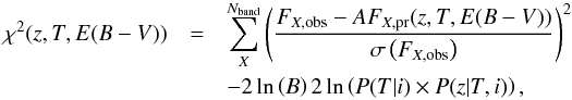 (11)where FX,obs is the observed flux in the X-band; FX,pr(z,T,E(B − V)) is the expected flux; Nband is equal to 5 for the CFHTLS and is equal to 6 for the LSST; and σ(FX,obs) is the observed flux uncertainty. The terms A and B come from the analytical marginalization over the normalization of the SEDs; they are defined as follows:
 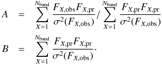 (12)In the following, the 3D posterior pdf is defined as ℒ = exp [− χ2 / 2]. It is computed for each galaxy on a 3D grid of 100 × 25 × 5 nodes in the (z, T, E(B − V)) parameter space. The values of the parameters z,T,E(B − V) lie in the intervals: [0,4.5], [0,50], and [0,0.3] respectively. Since we are controlling the domain of possible parameter values to match the ranges used to make the simulation, we are probably reducing the number of possible degeneracies in z,T,E(B − V) space. The SED library used for the photo-z reconstruction is the CWW+Kinney library, as described in Sect. 2.2.4. However, the templates have been optimized following the technique developed by Ilbert et al. (2006) when considering the CFHTLS spectro-photometric data; therefore, they naturally match the data better.
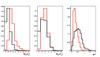 |
Fig. 9 Probability density function of the reduced variables Np(zp), Np(Tp), and g − r. The black lines correspond to P(μi|G) and the red lines to P(μi|O). |
The probability distribution is a function of three parameters. To derive the information on just one or two of the parameters, we integrate the distribution over all values of the unwanted parameter(s) in a process called marginalization. The marginalized 2D probability density functions of the parameters (z,T), (z,E(B − V)), (T,E(B − V)) and the marginalized 1D probability density function of each parameter are computed in this manner. Figure 8 shows an example of these probability density functions for a galaxy with a true redshift zs = 0.16, true type Ts = 45 (starburst), and true excess color E(B − V)s = 0.24. In many cases, the 3D posterior pdf is highly multimodal: therefore minimizing the χ2 with traditional algorithms, such as Minuit, often misses the global minimum. A scan of the parameter space is better suited to this application. Even a Markov Chain Monte Carlo (MCMC) method, which is usually more efficient than a simple scan, is not well suited to a multimodal 3D posterior pdf. Moreover, the production of the chains and their analysis in a 3D parameter space is slower than a scan. This example, where (zp − zs) / (1 + zs) = 0.27, corresponds to a catastrophic reconstruction. In this case, the parameters 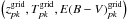 that maximize the 3D posterior pdf grid do not coincide with the ones that maximize the individual posterior probability density functions, namely the parameters
  .
.
3.2. Statistical test and rejection of outliers
In this section, we outline a statistical test that aims at rejecting some of the outlier galaxies, where |zp − zs| / (1 + zs) > 0.15. It is based on the characteristics of the 1D posterior probability density functions P(zpk), P(Tpk), and P(E(B − V)pk). The test is calibrated with a training sample, for which the true redshift is known (or the spectroscopic redshift in the case of real data). We use a subsample of our data (simulated or CFHTLS) for training. See Sects. 4.1 and 4.2 for full details. In the following, the LSST simulation for ten years of observation is considered to illustrate the method.
3.2.1. The probability density function characteristics
The variables considered to establish the statistical test are the following:
-
The number of peaks in the marginalized 1D posterior probabilitydensity functions denoted by Npk(θ), where θ is either z, T, or E(B − V);
-
When Npk > 1, the logarithm of the ratio between the height of the secondary peak over the primary peak in the 1D posterior probability density functions, denoted by RL(θ);
-
When Npk > 1, the ratio of the probability associated with the secondary peak over the probability associated with the primary peak in the 1D posterior probability density functions, denoted by Rpk(θ). The probability is defined as the integral between two minima on either side;
-
The absolute difference between the value of zpk and
 , as denoted by
  , where
  is the redshift that maximizes the posterior probability density function P(z);
 -
The maximum value of log (ℒ);
-
The colors, C = (u − g,g − r,r − i,i − z), in the case of CFHTLS, with an extra z − y term in the case of the LSST.
We denote the galaxies that are considered as outliers by O and the galaxies for which the redshift is well reconstructed by G in the following way:
-
O: |zp − zs| / (1 + zs) > 0.15
-
G: |zp − zs| / (1 + zs) < 0.15.
The set of variables defined in the list above are denoted by the vector μ. From a given training sample, we compute the distributions P(μi|O) and P(μi|G). For convenience, we adopt reduced variables that are renormalized to lie between 0 and 1. Distributions of some of the reduced variables are plotted in Fig. 9. It is clear that the distributions P(μi|G) and P(μi|O) are different. The probability that an outlier galaxy O presents more than three peaks in its posterior probability density function P(zp) is larger than for a well reconstructed galaxy G. A combination of these different pieces of information leads to an efficient test to distinguish between good and catastrophic reconstructions.
3.2.2. Likelihood ratio definition
To combine the information contained in the densities P(μi|G) and P(μi|O), we define the likelihood ratio variable LR: 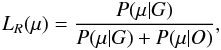 (13)where
 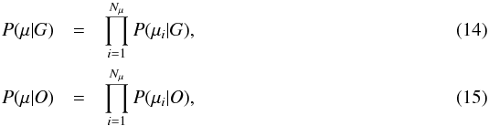 where Nμ is the number of components of μ. Here, the variables μi are assumed to be independent. The correlation matrix of the μi’s indeed shows a low correlation between the parameters. We approximate the two probabilities, P(G|μ) and P(O|μ), as the product of P(μ|G) and P(μ|O), neglecting the correlations, as our aim is just to define a variable for discriminating the two possibilities. The probability density functions, P(LR|G) and P(LR|O), are computed from the training sample and are displayed in Fig. 10. The results shown here are from the LSST simulation for ten years of observations with mX < m5,X. As expected, the two distributions are very different.
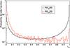 |
Fig. 10 Likelihood ratio distribution from the LSST simulation training sample. The probability density P(LR|G) in solid black and P(LR|O) in dashed red. |
The quality of a discrimination test, such as LR > LR,c, can be quantified by the acceptance Acc and rejection Rej rates: 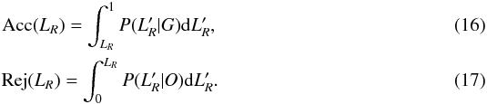 The evolution of Acc and Rej as functions of LR and Acc as a function of Rej is displayed in Fig. 11. The larger the difference between the curve Acc vs. Rej and the curve Acc = 1 − Rej, the higher the rejection power. Figure 11 shows that the method should work because the solid line lies far from the diagonal dotted line in the bottom left panel. A high value of LR is necessary to discard outliers; however, it should be chosen so a minimum of well-reconstructed galaxies are removed. The plots in Figs. 13 and 14, discussed below, show that there is a significant improvement when a cut on LR is applied.
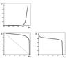 |
Fig. 11 From the LSST simulation training sample. Top panel: evolution of the rejection vs. LR. Bottom left-hand panel: evolution of the acceptance vs. the rejection. Bottom right-hand panel: evolution of the acceptance vs. LR. |
4. Photo-z performance with template-fitting
In the following sections, the ability of the statistical test, which is based on the LR variable, to construct a robust sample of galaxies with well-reconstructed redshifts is investigated in more detail for both the CFHTLS spectro-photometric data and the LSST simulation. The efficiency of the photo-z reconstruction is quantified by studying the distribution of (zp − zs) / (1 + zs) through the following:
-
bias: median that splits the sorted distribution in two equalsamples.
-
rms: the interquartile range (IQR)11. If the distribution is Gaussian, it is approximately equal to 1.35σ, where σ is the standard deviation.
-
η: the percentage of outliers for which |zp − zs| / (1 + zs) > 0.15.
Table 2 gives the LSST requirements for these values. Note that we use a different definition for the rms than the standard to match the definition stated for the LSST photo-z quality requirements.
4.1. Results for CFHTLS
In this section, the reconstruction of the photometric redshifts and the consequences of the selection on LR for the spectro-photometric data of CFHTLS are presented to validate the method. Two cases are considered:
-
Case A: the distributions P(μ|G) and P(μ|O) are computed from the data themselves.
-
Case B: the distributions P(μ|G) and P(μ|O) are computed from a simulation of the CFHTLS data, as explained in Sect. 2.3.2.
In both cases, the photo-z is computed from the real CFHTLS data. Figure 12 shows that the LR cut has a similar behavior if the distributions are determined from the simulation or from the data.
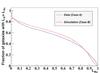 |
Fig. 12 Histogram of the number of galaxies from the CFHTLS sample with LR ≥ LR,c as a function of LR,c. The blue curve has been obtained with densities P(μ|G) and P(μ|O), as computed from the CFHTLS data themselves, whereas the red curve relies on densities obtained from the CFHTLS simulation. |
Figure 13 shows the performance of the template fitting photo-z reconstruction applied to the CHTLS data sample and the efficiency of the likelihood ratio LR cut. The results shown here have been obtained using the distributions for the likelihood ratio as computed from the data (case A); the results are similar if the distributions are computed from the simulations (case B). The 2D distributions of Δz as a function of spectroscopic redshift zs represented on the top part of the figure show that our simulation process using galaxy templates, K-corrections, reddening and the filter passbands do represent correctly the data, yielding reasonable photo-z reconstruction with no significant bias. One can also see a significant fraction of outliers, specially for galaxies with redshifts zs > 0.7. The likelihood ratio cut, LR > 0.6 here, removes most of the CHTLS outliers, as can be seen on Fig. 13, top-right, although with the cost of a low selection efficiency for high redshift galaxies (z > 0.9). The fraction of galaxies retained by the LR cut is shown on the lower left part of the Fig. 13, while the Δz distribution before and after LR cut is shown on lower-right part. Using the likelihood ratio criterion enhances significantly the photo-z performance since the RMS decreases from 0.16 to 0.09 and the outlier fraction from 12% to 2.8% between the full galaxy sample and the sub-sample of galaxies with LR > 0.6. However, the overall photo-z reconstruction performance and the LR cut efficiency is significantly below that on the LSST simulated data (see following subsection).
In Fig. 5 we see that the spectroscopic sample redshift coverage barely extends beyond z > 1.4. This means that when the LR selection was calibrated on the CFHTLS data, the sample was missing outlier galaxies with high redshifts that could be estimated erroneously to be at low redshifts, e.g. those subject to the degeneracy causing the Lyman break to be confused for the 4000 Å break. The LSST simulated data contains these degeneracies, however it would be good to test the LR selection method on real data out to higher redshifts in the future.
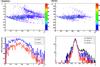 |
Fig. 13 CFHTLS spectro-photometric data: Top: Δz = zs − zp as a function of zs distribution for all galaxies (left) and for galaxies satisfying LR > LR,c = 0.6 (right). Bottom left: fraction of galaxies satisfying LR > LR,c = 0.2 (blue), 0.6 (red). Bottom right: Δz distribution for all galaxies and for galaxies satisfying the various LR cuts. |
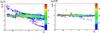 |
Fig. 14 Distribution of zp − zs versus zs for a simulated LSST catalog for all galaxies (left) and for galaxies with a likelihood ratio LR greater than 0.98 (right). |
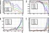 |
Fig. 15 LSST LR selection. Top: evolution of the fraction of detected galaxies satisfying LR > LR,c and the bias with zs. Bottom: evolution of the rms and η as a function of zs. The thick black lines represent the LSST requirements given in Table 2. Ten years of observations with the LSST is assumed. The values of LR,c are reported in the legend. |
4.2. Results for LSST
We use a total of 50 million galaxies in our simulated catalog. This catalog is divided into 5 different sets. Each set is separated into a test sample (2 million galaxies) and an analysis sample (8 million galaxies). In each set, the statistical test is performed on “observed” galaxies within the test sample, then the densities P(μ|G) and P(μ|O) are used to compute the value of LR for “observed” galaxies in the analysis sample. Performing the reconstruction on the 5 independent sets give us a measure of the fluctuation from a set to another and thus an estimate of the error on our reconstruction parameters. We performed the same analysis with 10 sets of twice less galaxies and measured the fluctuations to be very similar.
4.2.1. Observation in six bands
To test the method with best photometric quality we require each galaxy to be “observed” in each band with good precision mX < m5,X. This requirement leaves us with about 125 000 galaxies in the test sample and 500 000 in the analysis sample.
Figure 14 shows the 2D distributions from the LSST simulation of zp − zs as a function of zs for all the galaxies in the sample compared to the same distribution after performing an LR selection. It is clear that selecting on the likelihood ratio enhances the photometric redshift purity of the sample.
Figure 15 (the same as Fig. 13 for CFHTLS) shows the evolution with zs of the number of galaxies retained in the LSST sample, for each of the parameters listed above (bias, rms, η). This indicates the quality of the photo-z, for different values of LR,c.
The LSST specifications on the bias and rms (see Table 2) are fulfilled up to zs = 1.5 with only a low value of LR,c > 0.6. For redshifts greater than 1.5, a higher value of LR,c is required to reach the expected accuracy. There are two main reasons for this. Firstly, only a small percentage of the galaxies with zs > 1.5 are used to calibrate the densities P(μ|G) and P(μ|O), therefore the high-redshift galaxies do not have much weight in the calibration test. Secondly, the ratio between the height of the distribution P(LR|G) at LR = 0 and at LR = 1 tends to increase with the redshift, meaning that the purity of the test is degraded. Finally, only a very low value of LR,c > 0.2 is needed to enable η to meet LSST specifications for zs > 2.2.
The effect of a selection on the likelihood ratio LR can be compared to the effect of a selection on the apparent magnitude in the i-band, as shown in Fig. 16. The increase in the i-magnitude selection efficiency at large z shown in Fig. 16 (top) is due to the value of icut approaching the detection threshold. Performing a selection on a quantity other than magnitude, such as the likelihood ratio, ensures that “well measured” but faint galaxies are still included in the sample.
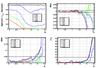 |
Fig. 16 LSST i magnitude selection. Top: evolution of the fraction of detected galaxies with i < icut and the bias with zs. Bottom: evolution of the rms and η as a function of zs. The thick black lines represent the LSST requirements given in Table 2. Ten years of observations with the LSST is assumed. The values of the i-magnitude cuts are reported in the legend. |
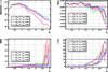 |
Fig. 17 LSST reconstruction for different Nm5 requirement. Top: evolution of the fraction of detected galaxies that satisfy the cuts (in the inset) and the bias with zs. Bottom: evolution of the rms and η as a function of zs. The thick black lines represent the LSST requirements given in Table 2. Ten years of observations with the LSST is assumed. The values of Nm5 and LR,c are reported in the legend. |
Of course requiring observation in six bands will exclude the u-band drop-out galaxies at high redshift, so the photo-z performance at these redshifts will be greatly affected by this requirement. The next section investigates the photo-z performance when observations are required in less than six bands.
4.2.2. Observation in five bands (and less)
The previous subsection demonstrated our results for good photometric data with mX < m5,X in all six bands of the LSST. To detect more galaxies and extend our reconstruction at higher redshift, we release the constraint on the number Nm5 of “well observed” bands having mX < m5,X. Both test and analysis sample are made of galaxies with mX < m5,X in at least Nm5 bands. We decreased Nm5 from 6 to 5, 4 and 3 and performed similar analysis to what was presented in the previous subsection. The comparison of the results indicates that the selection with Nm5 = 5 gives the best results. As we can see in Fig. 17, lowering Nm5 from 6 to 5 greatly increases the number of galaxies we keep in our sample without significantly degrading the reconstruction performance. The gain in the number of galaxies is presented in Table 5 and increases with redshift as expected.
For galaxies “observed” in only 5 bands, the band X which has mX > m5,X or is not observed at all (noise level) is the u band in 95% of the cases.
When requiring less than 5 bands, the results are worse or similar: to reconstruct decent photometric redshifts in this case we need to apply such a large value of LR for the selection that we reject nearly all the galaxies gained from the weaker requirement and even discard well-measured galaxies.
Figure 18 shows the comparison of the number of galaxies and photo-z performance (rms, bias, η) for a LR-selected sample (LR > 0.98) and a magnitude-selected sample (i < 24). While both samples satisfy the LSST science requirement given in Table 2, the LR selection is more efficient, since it retains a significantly larger number of galaxies, specifically for z > 1 (see Table 6). We do not present a comparison with a sample selected by a magnitude cut of i < 25.3, since it would not satisfy the LSST photo-z requirements, according to our simulation and photo-z reconstruction (as can be seen in Fig. 16).
Our choice of the value LR,c = 0.98, is a preliminary compromise between the quality of the redshift reconstruction and the number of measured galaxies. Increasing this threshold would lead to a smaller sample of galaxies with improved photometric performances. The final tuning will be driven by physics, depending on the impact of the cut on cosmological parameter determination and needs a more detailed and dedicated study.
LSST number of galaxies (LR,c = 0.98).
LSST number of galaxies, comparison between the selection on LR and the selection on i band magnitude.
5. Photo-z performance with neural network
It has been shown using the public code ANNz by Collister & Lahav (2004) that the photometric redshifts can be correctly estimated via a neural network. This technique, along with other empirical methods, requires a spectroscopic sample for which the apparent magnitudes and the spectroscopic redshifts are known.
The toolkit for multivariate analysis (Hoecker et al. 2007, TMVA) provides a ROOT-integrated environment for the processing, parallel evaluation, and application of multivariate classification and multivariate regression techniques. All techniques in TMVA belong to the family of supervised learning algorithms. They make use of training events, for which the desired output is known, to determine the mapping function that either describes a decision boundary or an approximation of the underlying functional behavior defining the target value. The mapping function can contain various degrees of approximations and may be a single global function, or a set of local models. Among artificial neural networks, many other algorithms, such as boosted decision trees or support vector machines, are available. An advantage of TMVA is that different algorithms can be tested at the same time in a very user-friendly way.
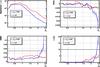 |
Fig. 18 LSST comparison between LR,c = 0.98 and i < 24 cuts. Top: evolution of the fraction of galaxies and the bias with zs. Bottom: evolution of the rms and η as a function of zs. The thick black lines represent the LSST requirements given in Table 2. Ten years of observations with the LSST is assumed. |
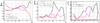 |
Fig. 19 Comparison between the template-fitting method and the neural network for CFHTLS data. The bias, the rms of the distribution of Δz / (1 + zs), and the parameter η are displayed as functions of the true redshift for the CFHTLS data. Data points are reported only if the number of galaxies in the sample is greater than ten. |
5.1. Method
The MultiLayer Perceptron (MLP) neural network principle is simple. It builds up a linear function that maps the observables to the target variables, which are the redshifts in our case. The coefficients of the function, namely the weights, are such that they minimize the error function which is the sum over all galaxies in the sample of the difference between the output of the network and the true value of the target. Two samples of galaxies, the training and the test sample, are necessary. The latter is used to test the convergence of the network and to evaluate its performance. It usually prevents overtraining of the network, which may arise when the network learns the particular feature of the training sample.
A neural network is built with layers and nodes. There are at least two layers, one for the input observables x and one for the target zMLP. Each node of a layer is related to all nodes from the previous layer with a weight w, which is the coefficient associated with the activation function A of each connection. The value  of the node k from the layer i + 1 is related to the values of all
  from the layer i:
 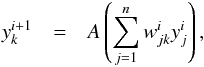 where n is the number of neurons in the i layer. For the purpose of this paper, the activation function A is a sigmoid. As an example, we examine the case where there is only one intermediate layer. Then the photometric redshift of the gth galaxy is estimated as follows:
 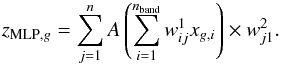 The error function is simply defined by
 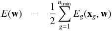 with
with  where ntrain is the number of galaxies in the training sample and g denotes the gth galaxy. At the first iteration, the weights have random values. The gradient descent method, which consists of modifying the weight value according to the derivative of E with respect to the weight, is used to minimize E. For example, we have after one iteration:
  The parameter α is the learning rate and has to be determined for each specific case. It must not be too large; otherwise, the steps are so large that the minimum of E is never reached. It must not be too small either; otherwise, too many iterations are required. The testing sample is used as a convergence and performance test. Indeed, the errors decrease with the number of iterations in the training sample but reach a constant value on the testing sample. Weights are finally kept when the errors on the testing sample reach a constant value.
For this non-exhaustive study on CFHTLS data, we have chosen the observables x = (m,σ(m)) and two layers of ten nodes each. The training sample contained 8000 randomly picked galaxies and the testing sample contained the remaining 6268 galaxies of the CFHTLS spectro-photometric catalog. In Fig. 19, the bias, rms, and the outlier rate η are compared for the template-fitting method and for the neural network. It is clear that the outlier rate is much smaller at all redshifts when the photo-z is estimated from the neural network. The dispersion of the photometric redshifts is also smaller for the neural network when compared to the template-fitting method. These characteristics are expected because the training sample is very similar to the test sample, whereas the template-fitting method uses only a small amount of prior information. Moreover, the apparent magnitudes in the template-fitting method are fitted with a model with SED templates, whereas no theoretical model has to be assumed to run the neural network. However, these attributes may be reversed if the two samples are different, as illustrated in Sect. 5.3. The overestimation of photo-z at low redshifts and underestimation at high redshifts, shown by the downward slope in the bias, can be attributed to attenuation bias. This is the effect of the measurement errors in the observed fluxes, resulting in the measured slope of the linear regression to be underestimated on average; see Freeman et al. (2009) for a full discussion of this bias. We note that the photo-z bias obtained from the template-fitting method has an opposite sign and is of the same amplitude to that obtained from the neural network method. Since we have reason to expect that the neural network has a downward slope in the bias, this indicates that the two estimators can be used complementarily. This is investigated in the next subsection.
5.2. Results for CFHTLS
Here, a possible combination of photo-z estimators (from the template-fitting method on the one hand and from the neural network on the other hand) is outlined. Even if the fraction of outlier galaxies is smaller with a neural network method than for the template-fitting method, using only the neural network to estimate the photo-z appears not to be sufficient to reach the stringent photo-z requirements for the LSST, especially when the spectroscopic sample is limited. Neural networks seem to produce a photo-z reconstruction that is slightly biased at both ends of the range (see Fig. 19). This is due to the galaxy under-sampling at low and very high redshifts in the training sample. When spectroscopic redshifts are available, it is therefore worth combining both estimators.
With the CFHTLS data, Fig. 20 shows that there is a correlation between zp − zMLP and zp − zs, where zp is the photo-z that is estimated with the template-fitting method. This correlation could be used to remove some of the outlier galaxies for which the difference between zp and zs is large, for example, by removing galaxies with around |zp − zMLP| ≥ 0.3. This correlation appears because the neural network is well trained, and therefore the photo-z is well estimated and zMLP becomes a good proxy for zs.
One can see an example of the impact of using both estimators zp and zMLP in Fig. 21. The distribution of zp − zs is plotted for three cases: LR > 0.9 only, |zp − zMLP| < 0.3 only and both cuts. There are fewer outlier galaxies from the first to the third case. By selecting with both variables, |zp − zMLP| and LR, we improve the photo-z estimation when compared to a selection based only on LR, or (to a lesser extent) only on |zp − zMLP|. This shows that neural networks have the capability to tag galaxies with an outlier template-fitted photo-z if the training sample is representative of the photometric catalog. However, this is difficult to achieve in practice because the training sample is biased in favor of bright, low redshift galaxies, which are most often the ones selected for spectroscopic observations.
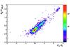 |
Fig. 20 2D histogram of zp − zMLP vs. zp − zs for the test sample of the CFHTLS data. |
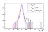 |
Fig. 21 Normalized histograms of zp − zs with LR > 0.9 (black curve), |zMLP − zp| < 0.3 (red curve) and both cuts (blue curve) for the CFHTLS data. |
5.3. Results for the LSST
For the LSST simulation, the network was composed of 2 layers of 12 nodes each; the training sample was composed of 10 000 galaxies and the testing sample of 20 000 galaxies. We found that increasing the size of the training sample above 10 000 showed no improvement in the precision of the training. We attribute this to the regularity of the simulation: the galaxies were drawn from a finite number of template SEDs. As soon as the sample represents all the galaxy types in the simulation, adding more galaxies does not help in populating the parameter space any longer.
A scatter plot of photo-z versus spectroscopic redshift is shown on the top panel of Fig. 22. The black points show the results from the template-fitting method, where a selection of LR > 0.98 was applied, and the red points show the results from the neural network as described above. The plot compares the photo-z performance of the neural network method and the template-fitting method on the simulated LSST data. Similar to Singal et al. (2011), we find that the neural network results in fewer outliers, although it has a larger rms for well-measured galaxies than the template-fitting method.
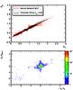 |
Fig. 22 Top panel: zp vs. zs with the template-fitting method in black (selection with LR > 0.98 ) and with the neural network in red for a LSST simulation of ten years of observations. Bottom panel: 2D histogram of zMLP − zp as a function of zp − zs. |
In the bottom panel of Fig. 22, the correlation between zp − zMLP and zp − zs is shown. Here, the correlation between both estimators is less useful for identifying outliers than it was for CFHTLS. This is presumably due to both the simulation and the fit being performed with the same set of galaxy template SEDs. This should significantly reduce the fraction of outliers compared to a case where the templates used to estimate zp do not correctly represent the real galaxies. For example, removing some of the templates from the zp fit reduces the photo-z quality, as demonstrated in Benítez (2000). Therefore, the existence of a strong correlation between zp − zMLP and zp − zs may be useful in diagnosing and mitigating problems with the SED template set.
It is difficult to obtain a spectroscopic sample of galaxies that is truly representative of the photometric sample in terms of redshifts and galaxy types (Cunha et al. 2012). For example, in the case of the LSST, the survey will be so deep that spectroscopic redshifts will be very hard to measure for the majority of faint galaxies or those within the “redshift desert”. Here, we briefly investigate the effect of having the spectroscopic redshift distribution of the training sample biased with respect to the full photometric sample.
The fact that the distribution of redshifts in the spectroscopic sample is different from the underlying distribution is often (confusingly) termed redshift bias. The consequence of this bias can be seen by modifying the efficiency of detection as a function of the redshift. The efficiency function is chosen to be  (18)and it is plotted in Fig. 23 (inset). This efficiency function is then used to bias the training sample and the test sample to compute new network weight coefficients. The photometric redshifts for another unbiased sample are then computed using these weights.
The scatter plot of zMLP − zs as a function of zs is shown in Fig. 23. We find that the photometric redshifts are well estimated as long as ϵ ≥ 0.2. This figure shows qualitatively that a bias in the training sample has a major impact on the photo-z reconstruction performance by the neural network, at least with the training method used here.
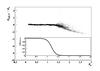 |
Fig. 23 zMLP − zs as a function of zs for the ten years of observations of the LSST. The curve in the inset shows the efficiency function ϵ as a function of the redshift, as it is used on the training sample to force a bias in the redshift selection. |
6. Discussion and future work
In regard to simulations undertaken here, there are a number of simplifications that will be reconsidered in future work. We discuss briefly some of these here.
-
Point source photometric errors: we have assumed photometric errors based on estimates valid for point sources, and since galaxies are extended sources, we expect the errors to be larger in practice. We made an independent estimate of the photometric errors as expected for the LSST, which includes the error degradation due to extended sources. For the median expected seeing, we found that the photometric error scales as σF / F = θ / 0.7, where σF is the error on the flux F, and θ is the size of the galaxy in arcseconds. The next round of simulations will therefore include a prescription for simulating galaxy sizes to improve our simulation of photometric errors. We will also compare our simple prescription to results obtained from the LSST image simulator (ImSim).
-
Galactic extinction (Milky Way): our current simulations effectively assume that i) Galactic extinction has been exactly corrected for, and ii) our samples of galaxies are all drawn from a direction of extremely low and uniform Galactic extinction. In practice, there will be a contribution to the photometric errors due to the imperfect correction of the Galactic extinction, and this error varies in a correlated way across the sky. More problematically, the extinction has the effect of decreasing the depth of the survey as a function of position on the sky. To account for these effects, we will construct a mapping between the coordinate system of our simulation and Galactic coordinates to apply the Galactic extinction in the direction to every galaxy in our simulation. We can use the errors in those Galactic extinction values to propagate an error to the simulated photometry.
-
Star contamination: M-stars have extremely similar colors to early type galaxies and can easily slip into photometric galaxy samples. Taking an estimate for the expected LSST star-galaxy separation quality, we plan to contaminate our catalog with stars. This could have an important effect by biasing the clustering signal of galaxies, since the contamination increases when the line of sight is close to the Galactic plane. It should also be possible to use the photo-z algorithm (either a template fitting or neural network type) to identify stars within the catalog.
-
Enhanced SEDs: our current simulations are probably more prone to problems with degeneracies in color space because we use a uniform interpolation between the main type SEDs. This may lead to poorer photometric redshifts than would be expected in reality, since galaxies might not exhibit such a continuous variation in SED type. In the future, we plan to implement a more realistic interpolation scheme and the use of more complete template libraries, such as synthetic spectral libraries.
-
Improved parameter estimation: a better characterization of the set of locally optimal parameters when determining the photo-z through the template fitting method might help us in rejecting outliers. We plan to further investigate this aspect in our future work.
7. Conclusion
We have developed a set of software tools to generate mock galaxy catalogs (as observed by the LSST or other photometric surveys), to compute photometric redshifts, and study the corresponding redshift reconstruction performance.
The validity of these mock galaxy catalogs was carefully investigated (see Sect. 2.3). We have shown that our simulation reproduces the photometric properties of the GOODS and CFHTLS observations well, especially in regard to the number count, magnitude and color distributions. We developed an enhanced template-fitting method for estimating the photometric redshifts, which involved applying a new selection method, the likelihood ratio statistical test, that uses the posterior probability functions of the fitted photo-z parameters (z, galaxy type, extinction ...) and the galaxy colors to reject galaxies with outlier redshifts.
This method was applied to both the CFHTLS data and the LSST simulation to derive photo-z performance, which was compared to the photo-z reconstruction by using a multilayer perceptron (MLP) neural network. We have shown how results from our template fitting method and the neural network might be combined to provide a galaxy sample of enriched objects with reliable photo-z measurements.
We find our enhanced template method produces photometric redshifts that are both realistic and meet LSST science requirements, when the galaxy sample is selected using the likelihood ratio statistical test. We have shown that a selection based on the likelihood ratio test performs better than a simple selection based on apparent magnitude, as it retains a significantly larger number of galaxies, especially at large redshifts (z ≳ 1), for a comparable photo-z quality.
We confirm that LSST requirements for photo-z determination, which consists of a (2−5)% dispersion on the photo-z estimate, with less than ~10% outliers can be met, up to redshift z ≲ 2.5. A number of enhancements for the mock galaxy catalog generation and photo-z reconstruction have been identified and were discussed in Sect. 8.
The photo-z computation presented here is designed for a full BAO simulation that aims to forecast the precision on the reconstruction of the dark energy equation-of-state parameter. This will be presented in a companion paper (Abate et al., in prep.).
Based on observations obtained with MegaPrime/MegaCam, a joint project of CFHT and CEA/DAPNIA at the Canada-France-Hawaii Telescope (CFHT), which is operated by the National Research Council (NRC) of Canada, the Institut National des Science de l’Univers of the Centre National de la Recherche Scientifique (CNRS) of France, and the University of Hawaii. This work is based in part on data products produced at TERAPIX and the Canadian Astronomy Data Centre as part of the Canada-France-Hawaii Telescope Legacy Survey, a collaborative project of NRC and CNRS.
The CFHTLS transmissions have been downloaded from http://www1.cadc-ccda.hia-iha.nrc-cnrc.gc.ca/community/CFHTLS-SG/docs/extra/filters.html
Acknowledgments
Thanks to Pierre Astier and Delphine Hardin for their advice on CFHTLS data, to Tomas Dahlen for his help on the simulation of the GOODS mock galaxy catalog and Eric Gawiser for his help with the IGM calculation. We also thank the LSST internal reviewers: Patricia Burchat, Andy Connolly and Sam Schmidt for their constructive criticism of the original paper draft.
References
- Abazajian, K. N., Adelman-McCarthy, J. K., Agüeros, M. A., et al. 2009, ApJS, 182, 543 [NASA ADS] [CrossRef] [Google Scholar]
- Baum, W. A. 1962, in IAU Symp. 15, ed. G. Cunliffe McVittie, 390 [Google Scholar]
- Benítez, N. 2000, ApJ, 536, 571 [NASA ADS] [CrossRef] [Google Scholar]
- Benítez, N., Gaztañaga, E., Miquel, R., et al. 2009, ApJ, 691, 241 [NASA ADS] [CrossRef] [Google Scholar]
- Bolzonella, M., Miralles, J.-M., & Pello’, R. 2000, A&A, 363, 476 [NASA ADS] [Google Scholar]
- Bruzual, G., & Charlot, S. 2003, MNRAS, 344, 1000 [NASA ADS] [CrossRef] [Google Scholar]
- Budavári, T., Szalay, A. S., Connolly, A. J., Csabai, I., & Dickinson, M. 2000, AJ, 120, 1588 [NASA ADS] [CrossRef] [Google Scholar]
- Cardelli, J. A., Clayton, G. C., & Mathis, J. S. 1989, ApJ, 345, 245 [NASA ADS] [CrossRef] [Google Scholar]
- Coleman, G. D., Wu, C., & Weedman, D. W. 1980, ApJS, 43, 393 [NASA ADS] [CrossRef] [Google Scholar]
- Collister, A. A., & Lahav, O. 2004, Publ. Astron. Soc. Pac., 116, 345 [NASA ADS] [CrossRef] [Google Scholar]
- Connolly, A., Csabai, I., Szalay, A., et al. 1995, AJ, 110, 2655 [NASA ADS] [CrossRef] [Google Scholar]
- Coupon, J., Ilbert, O., Kilbinger, M., et al. 2009, A&A, 500, 981 [NASA ADS] [CrossRef] [EDP Sciences] [Google Scholar]
- Cunha, C. E., Huterer, D., Busha, M. T., & Wechsler, R. H. 2012, MNRAS, 423, 909 [NASA ADS] [CrossRef] [Google Scholar]
- Dahlen, T., Mobasher, B., Somerville, R. S., et al. 2005, ApJ, 631, 126 [NASA ADS] [CrossRef] [Google Scholar]
- Dahlen, T., Mobasher, B., Jouvel, S., et al. 2008, AJ, 136, 1361 [NASA ADS] [CrossRef] [Google Scholar]
- Freeman, P. E., Newman, J. A., Lee, A. B., Richards, J. W., & Schafer, C. M. 2009, MNRAS, 398, 2012 [NASA ADS] [CrossRef] [Google Scholar]
- Garilli, B., Le Fèvre, O., Guzzo, L., et al. 2008, A&A, 486, 683 [NASA ADS] [CrossRef] [EDP Sciences] [Google Scholar]
- Hoecker, A., Speckmayer, P., Stelzer, J., et al. 2007 [arXiv:physics/0703039] [Google Scholar]
- Hogg, D. W., Baldry, I. K., Blanton, M. R., & Eisenstein, D. J. 2002 [arXiv:astro-ph/0210394] [Google Scholar]
- Ilbert, O., Arnouts, S., McCracken, H. J., et al. 2006, A&A, 457, 841 [NASA ADS] [CrossRef] [EDP Sciences] [Google Scholar]
- Ivezic, Z., Tyson, J. A., Acosta, E., et al. 2008 [arXiv:0805.2366] [Google Scholar]
- Jouvel, S., Kneib, J.-P., Ilbert, O., et al. 2009, A&A, 504, 359 [NASA ADS] [CrossRef] [EDP Sciences] [Google Scholar]
- Kinney, A. L., Calzetti, D., Bohlin, R. C., et al. 1996, ApJ, 467, 38 [NASA ADS] [CrossRef] [Google Scholar]
- Le Fevre, O., Guzzo, L., Meneux, B., et al. 2005, A&A, 439, 877 [NASA ADS] [CrossRef] [EDP Sciences] [Google Scholar]
- Lilly, S., Le Fèvre, O., Renzini, A., et al. 2007, ApJS, 172, 70 [NASA ADS] [CrossRef] [Google Scholar]
- LSST Science Collaboration 2009 [arXiv:0912.0201] [Google Scholar]
- Madau, P. 1995, ApJ, 441, 18 [NASA ADS] [CrossRef] [Google Scholar]
- Matthews, D. J., & Newman, J. A. 2010, ApJ, 721, 456 [NASA ADS] [CrossRef] [Google Scholar]
- Matthews, D. J., & Newman, J. A. 2012, ApJ, 745, 180 [NASA ADS] [CrossRef] [Google Scholar]
- Newman, J. A., Cooper, M. C., Davis, M., et al. 2013, ApJS, 208, 5 [Google Scholar]
- Petry, C. E., Miller, M., Cook, K. H., et al. 2012, in AAS Meeting Abstracts, 219, 156.09 [Google Scholar]
- Puschell, J., Owen, F., & Laing, R. 1982, in Extragalactic Radio Sources, eds. D. S. Heeschen, & C. M. Wade, IAU Symp., 97, 423 [Google Scholar]
- Sheldon, E. S., Cunha, C. E., Mandelbaum, R., Brinkmann, J., & Weaver, B. A. 2012, ApJS, 201, 32 [NASA ADS] [CrossRef] [Google Scholar]
- Singal, J., Shmakova, M., Gerke, B., Griffith, R. L., & Lotz, J. 2011, PASP, 123, 615 [NASA ADS] [CrossRef] [Google Scholar]
- Vanzella, E., Cristiani, S., Fontana, A., et al. 2004, A&A, 423, 761 [NASA ADS] [CrossRef] [EDP Sciences] [Google Scholar]
All Tables
Number of visits and 5σ limiting apparent magnitudes (point sources), for one year and ten years of LSST operation (Ivezic et al. 2008; Petry et al. 2012).
LSST photo-z requirements for the high signal-to-noise “gold sample” subset, which is defined as having i < 25.3.
Number of galaxies that are both observed photometrically with the CFHTLS survey and spectroscopically.
LSST number of galaxies, comparison between the selection on LR and the selection on i band magnitude.
All Figures
|
Fig. 1 SED templates are linearly interpolated from the original six templates from Coleman et al. (1980) and Kinney et al. (1996). The original templates are drawn in red. |
| In the text | |
|
Fig. 2 LSST transmission curves shown by the solid lines and CFHTLS transmissions shown by the dashed lines. The transmission includes the transmission of the filter itself, the expected CCD quantum efficiency, and the telescope optical throughput. |
| In the text | |
|
Fig. 3 Histograms of the apparent magnitude in the R band comparing the GOODS simulated data (black points with error bars) to the actual GOODS data (red stars). We note that there may be a systematic shift in all data points in the x-axis direction up to R ≲ 0.05 mag due to differences between the simulation and data filter zero points. |
| In the text | |
|
Fig. 4 Histograms of the B − R term for different apparent magnitude ranges. Left-hand panel (20 < R < 22) corresponds to the bright galaxies and right-hand panel (24 < R < 25.5) corresponds to the very faint galaxies. The solid black lines correspond to the simulation and the solid red lines correspond to the GOODS data. The dotted colored lines correspond to the main spectral types in the simulation. |
| In the text | |
|
Fig. 5 Redshift distribution of the spectroscopic sample for the different CFHTLS fields. The histograms are stacked. |
| In the text | |
|
Fig. 6 Color–color plots showing the relation between CFHTLS data (black dots) and the distribution expected from our SED template set (red dots). |
| In the text | |
|
Fig. 7 Left-hand side: cumulative distribution of the apparent magnitude in the i band for the LSST simulation compared to the Sloan Digital Sky Survey (SDSS) measurement from the Stripe 82 region (cf. Abazajian et al. 2009). The statistical error bars from the data are smaller than the dots size. Right-hand side: redshift distribution of galaxies for the LSST: i < 24, i < 25 with σi < 0.2 (solid red, solid black curves respectively); i < 27 with S ! N > 5 in at least the i band for one and ten years of observations (dotted and solid magenta respectively); S ! N > 5 in all bands for one and ten years of observations (dotted and solid blue respectively). |
| In the text | |
|
Fig. 8 Example of photometric computation for a simulated galaxy observed with the LSST in six bands at 5σ for ten years of observation. The 2D distributions correspond to the posterior probability density functions marginalized over the remaining parameter, and the 1D distributions correspond to the posterior probability density functions marginalized over the two remaining parameters. The top middle panel corresponds to the value of the input parameters. On the top right-hand panel, the index grid denotes the parameters that maximize the 3D posterior probability density function on the grid, and on the middle right-hand panel, the index marg denotes the parameters that maximize the 1D posterior probability density functions. The size of the grid cells has been reduced, and the zp axis has been shortened compared to the size of the grid that is usually used to compute the likelihood function. |
| In the text | |
|
Fig. 9 Probability density function of the reduced variables Np(zp), Np(Tp), and g − r. The black lines correspond to P(μi|G) and the red lines to P(μi|O). |
| In the text | |
|
Fig. 10 Likelihood ratio distribution from the LSST simulation training sample. The probability density P(LR|G) in solid black and P(LR|O) in dashed red. |
| In the text | |
|
Fig. 11 From the LSST simulation training sample. Top panel: evolution of the rejection vs. LR. Bottom left-hand panel: evolution of the acceptance vs. the rejection. Bottom right-hand panel: evolution of the acceptance vs. LR. |
| In the text | |
|
Fig. 12 Histogram of the number of galaxies from the CFHTLS sample with LR ≥ LR,c as a function of LR,c. The blue curve has been obtained with densities P(μ|G) and P(μ|O), as computed from the CFHTLS data themselves, whereas the red curve relies on densities obtained from the CFHTLS simulation. |
| In the text | |
|
Fig. 13 CFHTLS spectro-photometric data: Top: Δz = zs − zp as a function of zs distribution for all galaxies (left) and for galaxies satisfying LR > LR,c = 0.6 (right). Bottom left: fraction of galaxies satisfying LR > LR,c = 0.2 (blue), 0.6 (red). Bottom right: Δz distribution for all galaxies and for galaxies satisfying the various LR cuts. |
| In the text | |
|
Fig. 14 Distribution of zp − zs versus zs for a simulated LSST catalog for all galaxies (left) and for galaxies with a likelihood ratio LR greater than 0.98 (right). |
| In the text | |
|
Fig. 15 LSST LR selection. Top: evolution of the fraction of detected galaxies satisfying LR > LR,c and the bias with zs. Bottom: evolution of the rms and η as a function of zs. The thick black lines represent the LSST requirements given in Table 2. Ten years of observations with the LSST is assumed. The values of LR,c are reported in the legend. |
| In the text | |
|
Fig. 16 LSST i magnitude selection. Top: evolution of the fraction of detected galaxies with i < icut and the bias with zs. Bottom: evolution of the rms and η as a function of zs. The thick black lines represent the LSST requirements given in Table 2. Ten years of observations with the LSST is assumed. The values of the i-magnitude cuts are reported in the legend. |
| In the text | |
|
Fig. 17 LSST reconstruction for different Nm5 requirement. Top: evolution of the fraction of detected galaxies that satisfy the cuts (in the inset) and the bias with zs. Bottom: evolution of the rms and η as a function of zs. The thick black lines represent the LSST requirements given in Table 2. Ten years of observations with the LSST is assumed. The values of Nm5 and LR,c are reported in the legend. |
| In the text | |
|
Fig. 18 LSST comparison between LR,c = 0.98 and i < 24 cuts. Top: evolution of the fraction of galaxies and the bias with zs. Bottom: evolution of the rms and η as a function of zs. The thick black lines represent the LSST requirements given in Table 2. Ten years of observations with the LSST is assumed. |
| In the text | |
|
Fig. 19 Comparison between the template-fitting method and the neural network for CFHTLS data. The bias, the rms of the distribution of Δz / (1 + zs), and the parameter η are displayed as functions of the true redshift for the CFHTLS data. Data points are reported only if the number of galaxies in the sample is greater than ten. |
| In the text | |
|
Fig. 20 2D histogram of zp − zMLP vs. zp − zs for the test sample of the CFHTLS data. |
| In the text | |
|
Fig. 21 Normalized histograms of zp − zs with LR > 0.9 (black curve), |zMLP − zp| < 0.3 (red curve) and both cuts (blue curve) for the CFHTLS data. |
| In the text | |
|
Fig. 22 Top panel: zp vs. zs with the template-fitting method in black (selection with LR > 0.98 ) and with the neural network in red for a LSST simulation of ten years of observations. Bottom panel: 2D histogram of zMLP − zp as a function of zp − zs. |
| In the text | |
|
Fig. 23 zMLP − zs as a function of zs for the ten years of observations of the LSST. The curve in the inset shows the efficiency function ϵ as a function of the redshift, as it is used on the training sample to force a bias in the redshift selection. |
| In the text | |
Current usage metrics show cumulative count of Article Views (full-text article views including HTML views, PDF and ePub downloads, according to the available data) and Abstracts Views on Vision4Press platform.
Data correspond to usage on the plateform after 2015. The current usage metrics is available 48-96 hours after online publication and is updated daily on week days.
Initial download of the metrics may take a while.