| Issue |
A&A
Volume 555, July 2013
|
|
|---|---|---|
| Article Number | A136 | |
| Number of page(s) | 11 | |
| Section | The Sun | |
| DOI | https://doi.org/10.1051/0004-6361/201321628 | |
| Published online | 12 July 2013 | |
Evaluating local correlation tracking using CO5BOLD simulations of solar granulation⋆
Leibniz-Institut für Astrophysik Potsdam,
An der Sternwarte 16,
14482
Potsdam,
Germany
e-mail: This email address is being protected from spambots. You need JavaScript enabled to view it.
; This email address is being protected from spambots. You need JavaScript enabled to view it.
; This email address is being protected from spambots. You need JavaScript enabled to view it.
Received: 2 April 2013
Accepted: 21 May 2013
Abstract
Context. Flows on the solar surface are intimately linked to solar activity, and local correlation tracking (LCT) is one of the standard techniques for capturing the dynamics of these processes by cross-correlating solar images. However, the link between contrast variations in successive images to the underlying plasma motions has to be quantitatively confirmed.
Aims. Radiation hydrodynamics simulations of solar granulation (e.g., CO5BOLD) provide access to both the wavelength-integrated, emergent continuum intensity and the three-dimensional velocity field at various heights in the solar atmosphere. Thus, applying LCT to continuum images yields horizontal proper motions, which are then compared to the velocity field of the simulated (non-magnetic) granulation. In this study, we evaluate the performance of an LCT algorithm previously developed for bulk-processing Hinode G-band images, establish it as a quantitative tool for measuring horizontal proper motions, and clearly work out the limitations of LCT or similar techniques designed to track optical flows.
Methods. Horizontal flow maps and frequency distributions of the flow speed were computed for a variety of LCT input parameters including the spatial resolution, the width of the sampling window, the time cadence of successive images, and the averaging time used to determine persistent flow properties. Smoothed velocity fields from the hydrodynamics simulation at three atmospheric layers (log τ = −1, 0, and +1) served as a point of reference for the LCT results.
Results. LCT recovers many of the granulation properties, e.g., the shape of the flow speed distributions, the relationship between mean flow speed and averaging time, and also – with significant smoothing of the simulated velocity field – morphological features of the flow and divergence maps. However, the horizontal proper motions are grossly underestimated by as much as a factor of three. The LCT flows match best the flows deeper in the atmosphere at log τ = +1.
Conclusions. Despite the limitations of optical flow techniques, they are a valuable tool in describing horizontal proper motions on the Sun, as long as the results are not taken at face value but with a proper understanding of the input parameter space and the limitations inherent to the algorithm.
Key words: Sun: granulation / convection / methods: numerical / techniques: image processing / hydrodynamics
Movies are available in electronic form at http://www.aanda.org
© ESO, 2013
1. Introduction
The interaction of flow and magnetic fields on the solar surface is linked to the ever-changing appearance of solar activity. Various techniques have been developed to measure photospheric proper motions. November & Simon (1988) introduced the local correlation tracking (LCT) technique to the solar physics community, which had previously been developed by Leese et al. (1971) to track cloud motion from geosynchronous satellite data. Since then many variants of the LCT algorithm have been used to quantify horizontal flow properties in the solar photosphere and chromosphere. Verma & Denker (2011) adapted the LCT algorithm to G-band images captured by the Solar Optical Telescope (SOT, Tsuneta et al. 2008) on board the Japanese Hinode mission (Kosugi et al. 2007) with the aim for establishing a standard method for bulk-processing time-series data. Beauregard et al. (2012) modified the same algorithm for continuum images of the Helioseismic and Magnetic Imager (HMI, Scherrer et al. 2012) on board the Solar Dynamics Observatory (SDO, Pesnell et al. 2012).
Besides images, magnetograms are often used to determine horizontal proper motions. Welsch et al. (2007) tested and compared various techniques: minimum-energy fitting (MEF, Longcope 2004), the differential affine velocity estimator (DAVE, Schuck 2006), Fourier local correlation tracking (FLCT, Welsch et al. 2004), the induction method (IM, Kusano et al. 2002), and induction local correlation tracking (ILCT Welsch et al. 2004). These algorithms were applied to simulated magnetograms using the anelastic MHD code by Lantz & Fan (1999). However, the results were not conclusive, because all methods showed considerable errors in estimating velocities. In general, MEF, FLCT, DAVE, IM, and ILCT lead to similar results with a slightly better performance of DAVE in estimating direction and magnitude of the velocities, but the magnetic flux energy and helicity were recovered better using MEF.
The study by Welsch et al. (2007) was extended by Chae & Sakurai (2008), who tested three optical flow methods, i.e., LCT, DAVE, and the nonlinear affine velocity estimator (NAVE, Schuck 2005), using simulated, synthetic, and Hinode magnetograms. NAVE performed well in detecting subpixel, superpixel, and nonuniform motions, whereas LCT had problems in sensing non-uniform motions, and DAVE displayed deficiencies in estimating superpixel motions. However, LCT is the fastest and NAVE the slowest algorithm. Chae & Sakurai (2008) proposes to select smaller sampling windows to get more detailed velocity maps and to lessen the computational demands.
Rieutord et al. (2001) applied LCT and feature tracking to photospheric images derived from numerical simulations of compressible convection and concluded that both methods fail to represent the velocity field on spatial scales smaller than 2500 km and temporal scales shorter than 30 min. In addition, simulated continuum images (Vögler et al. 2005) were used by Matloch et al. (2010) to characterize properties of mesogranulation. However, to the best of our knowledge no systematic study has been carried out based on simulated continuum images to evaluate the reliability, accuracy, and parameter dependence of LCT. In this study, we present the results of rigorously testing the LCT algorithm of Verma & Denker (2011) using CO5BOLD simulations of solar convection (Freytag et al. 2012). Ultimately, we want to answer the question: How much of the underlying physics can be captured using optical flow methods?
2. CO5BOLD simulation of solar granulation
Radiation hydrodynamic simulations of solar and stellar surface convection have become increasingly realistic producing many aspects of observations. The CO5BOLD code (Freytag et al. 2012) offers a unique opportunity to evaluate a previously developed LCT algorithm (Verma & Denker 2011) and to explore the parameter space for tracking solar fine-structure, in particular for scrutinizing the multi-scale (time and space) nature of solar surface convection. CO5BOLD simulations have been computed for a variety of solar models. The present CO5BOLD simulations are non-magnetic, i.e., pure radiation hydrodynamics. Here, the grid dimensions of the simulation are 400 × 400 × 165 and the horizontal cell size is 28 km × 28 km with the vertical grid spacing increasing with depth from 12 km in the photosphere to 28 km in the lower part of the model, resulting in a box with a size of 11.2 × 11.2 × 3.1 Mm3. Even larger simulation boxes are needed to study convective signatures on larger spatial scales. Matloch et al. (2010), for example, extracted characteristic properties of mesogranulation (e.g., size and lifetime) from three-dimensional hydrodynamical simulations (MURaM code, Vögler et al. 2005).
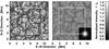 |
Fig. 1 First (left) and one-hour averaged (right) images with 400 × 400 pixels and an image scale of 28 km pixel-1 taken from a CO5BOLD time series of solar granulation. Because of the Gaussian kernels (in the insert lower right corner) of 128 × 128 pixels used as sampling windows, the original image size was reduced by 128 pixels. The white squares mark the region with a size of 273 × 273 pixels that remains after the LCT computation. |
In the first part of this study, we analyze a time series of snapshots of the bolometric emergent continuum intensity based on a high-resolution CO5BOLD simulation of granulation. The 140-min time series comprises 832 images with a size of 400 × 400 pixels at a time cadence of Δt = 10 s. The image scale is 28 km pixel-1. The first image of the time series is shown in the left panel of Fig. 1. The intensity contrast of image is about 15.9%. Taking the average of 360 images (right panel of Fig. 1) reduces the contrast to about 5.3% but the appearance of the intensity pattern still remains granular without any indication of long-lived features. In general, the modulation transfer function (MTF) of the telescope has to be considered when comparing simulated with observed data (Wedemeyer-Böhm & Rouppe van der Voort 2009). However, we did not convolve the images with the point spread function to include the instrumental image degradation, because the fine-structure contents of an image are given by the Fourier phases and not the Fourier amplitudes. Modifying the Fourier amplitudes in granulation images or changing the shape and width of the LCT sampling window are intertwined and could be in principle disentangled but at the cost of complexity. In the second part of the data analysis, we compare the LCT results with the underlying velocity structure of the CO5BOLD simulations. The time cadence of the velocity data is, however, reduced to Δt = 20 s. For an impartial comparison, all LCT maps were computed first before confronting them with the intrinsic velocity field of the CO5BOLD simulations.
3. Local correlation tracking
Flow maps were computed using the LCT algorithm described in Verma & Denker (2011) but initial image alignment, subsonic filtering, and geometric correction were excluded. An important difference between the Hinode and CO5BOLD data is the image scale of 80 and 28 km pixel-1, respectively. Sampling windows and filter kernels of 32 × 32 pixels were the choice for processing Hinode G-band images because the computation time should be kept to a minimum for bulk-processing of time-series data. However, for this study we opted for sizes of 128 × 128 pixels to adapt to the higher spatial resolution of the simulated granulation images and to extend our parameter study to include broader sampling windows. The drawback is of course a much increased computation time. In principle, smaller sampling windows could have been chosen for smaller full width at half maximum (FWHM) but for consistency, we decided not to change window or kernel sizes. In a direct comparison with the previous work of Verma & Denker (2011), these small differences are of no concern.
A 128 × 128-pixel Gaussian kernel with an FWHM = 1200 km is shown as an illustration in the lower-right corner of the right panel in Fig. 1. If not otherwise noted, this kernel is used as a high-pass filter, even though this is not strictly necessary in the absence of strong intensity gradients (e.g., umbra-penumbra or granulation-penumbra boundaries) and gentler slopes introduced by the limb darkening. Because of such sampling windows and kernels the size of the computed LCT maps was reduced to 273 × 273 pixels from the 400 × 400 pixels of the original images, which is indicated in Fig. 1 by white square boxes.
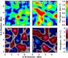 |
Fig. 2 Average speed (top) and divergence (bottom) maps for the first (left) and last (right) hour of the time series computed using a time cadence of Δt = 60 s and a Gaussian sampling window with an FWHM = 1200 km. The direction and magnitude of the horizontal flows are plotted over the divergence maps as arrows, for which a velocity of 0.5 km s-1 corresponds to exactly the grid spacing. The values displayed at the top are the mean speed |
4. Results
4.1. Persistent flows and the duration of time averages
One application of LCT techniques is to uncover persistent horizontal proper motions. The imprint of solar convection results in a photospheric flow field with different spatial scales: granulation 1–2 Mm, mesogranulation 3–10 Mm, and supergranulation ~30 Mm (Muller et al. 1992). The LCT method recovers the corresponding flow features from time series of photospheric images. This raises the question, if similar signatures are present in the simulated time series of granulation.
In Fig. 2, we computed flow (top row) and divergence (bottom row) maps for the first (left column) and last (right column) hour of the time series. We chose a time cadence of Δt = 60 s and a Gaussian sampling window with an FWHM = 1200 km and then averaged the individual flow maps over ΔT = 1 h to facilitate easier comparison with the study of Verma & Denker (2011). This choice of input parameters produced the most reliable results when previously applied to Hinode G-band images. The mean speeds  and their standard deviations σv are 0.51 ± 0.20 km s-1 and 0.68 ± 0.31 km s-1 for the first and last hour, respectively. The mean speed in the later case is higher by 33% because of a large structure with high velocities in the top-left quarter of the flow map. The divergence of a flow field with velocity components (vx,vy) is computed as . On average the divergence values are two times higher than the ones for Hinode G-band images discussed in Verma & Denker (2011). The superimposed flow vectors clearly indicate the locations of the diverging and converging flows.
Neither the two flow nor the two divergence maps bear any resemblance to another suggesting that after about one hour persistent flow features are no longer present in the CO5BOLD time series. The absence of meso- or supergranular features is, however, expected considering both the horizontal dimensions and the depth of the simulation box. Interestingly, strong flow features will still be present even after averaging for one hour, which points to the necessity of longer time series for assessing convective flow properties on larger spatial scales.
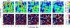 |
Fig. 3 Speed (top) and divergence (bottom) maps averaged over time intervals of ΔT = 15–120 min. The LCT maps were computed using a time cadence of Δt = 60 s and a Gaussian sampling window with an FWHM = 1200 km. |
The time dependence of the average flow field is depicted in Fig. 3 along with the corresponding divergence maps. These maps were computed with the same input parameters as in Fig. 2 but in this case with different time intervals ΔT = 15–120 min over which the individual flow maps were averaged. Proper motions of single granules are well captured when flow maps are averaged over ΔT = 15 and 30 min, which is evident from the speed maps containing mostly features of typical granular size. However, contributions to the flow field from separate granules are averaged out over longer time intervals ΔT, but some long-lived features might survive the averaging process. Most notably, a high-velocity feature with negative divergence (converging flows) remains in the central part of the maps. It first appears at 15 min as an appendage to a stronger flow kernel, then separates from the kernel (30–60 min), before becoming the only strong flow kernel at 90 min, and fading away after about 120 min. This behavior resembles flow patterns encountered at the vertices of supergranular cells. However, in real observations the lifetime of such a flow kernel with converging horizontal motions is much longer. Despite the tendency of lower divergence values for increasing ΔT, the divergence values are still significantly higher than the values given by Verma & Denker (2011).
The more than 30% decrease of the average flow speed from 0.70 km s-1 in the 15-min map to 0.46 km s-1 in the 120-min map is of the same order as the 25% difference found for the two one-hour averaged flow maps in Fig. 2. Furthermore, the extended flow feature in the right panel of Fig. 2 is absent in the 120-min map of Fig. 3 pointing to the importance of the vectorial summation (constructive and destructive) of the individual flow maps. Taken together, both facts serve as a reminder that we must treat the mean speed values of different sequences with caution when comparing them. In addition, the large variance of reported speed values in the literature might also have its origin in the stochastic nature of granulation and not only in the choice of LCT input parameters. In the following, only data for the first hour of the time series were analyzed.
4.2. Convergence properties of the mean flow speeds
Hinode is the most prolific data source for high-resolution solar images, and G-band images with 2 × 2-pixel binning and an image scale of about 80 km pixel-1 are the most common image type. Hence, the LCT algorithm of Verma & Denker (2011) was developed for bulk-processing of these images leading to an optimal set of LCT input parameters: time cadence Δt = 60–90 s, Gaussian sampling window with an FWHM = 1200 km, and averaging time ΔT = 1 h. Beauregard et al. (2012) showed that this algorithm is easily adaptable to images with a coarser spatial sampling, e.g., continuum images of the SDO/HMI. In the following, we use CO5BOLD simulation data to cross-check the aforementioned input parameters.
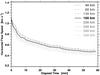 |
Fig. 4 Average horizontal flow speed as a function of the elapsed time. The maps were computed using a Gaussian sampling window with an FWHM = 1200 km and time cadence Δt = 60 s. Before computing the cross-correlations, the images were convolved with a Gaussian kernel FWHM = 40–320 km to degrade the spatial resolution of the images. The increasing FWHM values are presented as progressively lighter shades of gray. The dash-dotted and dashed lines represents values above and below optimal parameter (FWHM = 160 km), respectively. The black solid line is used to depict result for the FWHM = 160 km, which is the typical spatial resolution of most Hinode G-band images (see Verma & Denker 2011). |
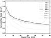 |
Fig. 5 Average horizontal flow speed as a function of the elapsed time. The maps were computed using a Gaussian sampling window with an FWHM = 1200 km and time cadence Δt = 10–480 s. The increasing time cadences Δt are presented as progressively lighter shades of gray. The black solid line is depicting the result for the time cadence Δt = 60 s, which has been identified in Verma & Denker (2011) as an optimal choice for tracking horizontal proper motions in Hinode G-band time-series data. |
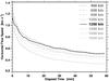 |
Fig. 6 Average horizontal flow speed as a function of the elapsed time. The maps were computed using a time cadence Δt = 60 s and Gaussian sampling window with various FWHM = 400–1800 km. The increasing FWHM values are presented as progressively lighter shades of gray. The black solid line is used to depict the result for a Gaussian sampling window with an FWHM = 1200 km, which has been identified in Verma & Denker (2011) as an optimal choice for tracking horizontal proper motions in Hinode G-band time-series data. |
First, to study the effects of spatial resolution, we degraded the original images with an image scale of 28 km pixel-1 by convolving them with Gaussian kernels of FWHM = 40–320 km but without correcting the telescope’s MTF (cf., Wedemeyer-Böhm & Rouppe van der Voort 2009). We computed the mean horizontal flow speed as a function of the elapsed time, as shown in Fig. 4. The elapsed time corresponds to the number of flow maps averaged. These temporal averages were carried out up to ΔT = 1 h. The Gaussian sampling window with an FWHM = 1200 km and time cadence Δt = 60 s were kept constant. Different shades of gray from dark to light indicate increasingly larger FWHM. The black curve (FWHM = 160 km) corresponds to the spatial resolution of the Hinode G-band images. The diffraction-limited resolution of the 0.5-m Hinode/SOT according to the Rayleigh criterion is 1.22·λ/D = 0.22″ at λ430 nm or 160 km on the solar surface. Therefore, even with 2 × 2-binning, Hinode G-band images are still critically sampled (Nyquist theorem). In the following, we use v28 to indicate velocities that were derived from the full-resolution simulated images, while v80 refers to velocities based on smoothed simulated images, which provide the link to G-band images (see Verma & Denker 2011).
It takes about 5–10 min before the slope of the curves changes, and after 15–20 min the curves level out and approach an asymptotic value. Changing the slope is directly related to the lifetime of individual granules, and it takes several lifetimes to reveal any longer-lasting flow features. In addition, all the curves are stacked on top of each other without crossing any other curve at any point. The mean flow speed decreases monotonically by about 0.1 km s-1 when reducing the FWHM of the Gaussian filter kernel from 40 to 320 km. Evidently, in images with high spatial resolution, the LCT algorithm picks up fine-structure such as the corrugated boundaries of granules, fragments of exploding granules, and the occasional bright points. These feature have either intrinsically higher speeds or high contrasts, thus biasing the cross-correlation algorithm to higher velocities.
Second, we change the time cadences in the range of Δt = 10–480 s while keeping the FWHM = 1200 km of the Gaussian sampling window and the spatial resolution of 28 km pixel-1 constant as depicted in Fig. 5. Shades of gray from dark to light indicate longer time cadences. The black curve corresponds to the optimal LCT parameter Δt = 60 s for G-band images. This curve exhibits the highest mean speed except for very short averaging times. For shorter time cadences Δt = 10–30 s, the mean velocity profiles differ only slightly and monotonically approach the 60-s profile. Starting with the 90-s profile, the mean velocities drastically drop. If the time cadence is too short, then granules have not evolved sufficiently to provide a strong cross-correlation signal. If, on the other hand, the time cadence becomes too long, then granules have either evolved too much or completely disappeared so that their horizontal proper motions are no longer properly measured. Already a time cadence of Δt = 90 s is a compromise, but many G-band time series are acquired with more than 60 s between successive images. These findings are consistent with a similar parameter study for Hinode G-band images (see Fig. 3 of Verma & Denker 2011) and independently corroborate that the CO5BOLD simulation reproduces essential flow characteristics of solar granulation.
Third, the last important input parameter is the FWHM of the Gaussian sampling window, which was adjusted in the range from 400 to 1800 km (see Fig. 6), while maintaining a constant time cadence (Δt = 60 s) and image scale (28 km pixel-1). The reference profile (FWHM = 1200 km) is once more shown as a black curve. Interestingly, profiles with small FWHM = 400 and 600 km start at high velocities, then quickly drop, while intersecting all other profiles. These sampling windows track fine structures with high velocities but the lack of large, coherent structures (i.e., at least one entire granule) rapidly diminishes the mean flow speed. The highest flow speeds in the asymptotic part of the mean speed profiles are found for FWHM = 800 and 1000 km. These profiles are very similar but cut across each other at an averaging time of ΔT ≈ 14 min. Starting at an FWHM = 1200 km, the mean speed profiles are again systematically arranged without any intersection. Once the sampling window is sufficiently large to encompass several granules, their stochastic motions tend to reduce the average flow speed.
In summary, the mean speed profiles in Figs. 4–6 confirm that for an image scale of 80 km pixel-1 the LCT input parameters (averaging time ΔT = 1 h, time cadence Δt = 60 s, and a Gaussian sampling window with an FWHM = 1200 km) are indeed the most reasonable choice to derive horizontal proper motions from Hinode G-band images.
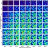 |
Fig. 7 Horizontal flow speed maps (one-hour averages) computed with time cadences Δt = 10–480 s (bottom to top) and Gaussian kernels with an FWHM = 400–1800 km (left to right). Displayed at the top of the panels are the mean speed |
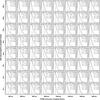 |
Fig. 8 Relative frequency distributions of horizontal flow speeds computed with time cadences Δt = 10–480 s (bottom to top) and Gaussian sampling windows with an FWHM = 400–1800 km (left to right). The three vertical lines mark the position of median vmed (solid), mean |
4.3. Morphology of flow maps and frequency distributions of flow speeds
Two-dimensional maps of the flow speed offer another approach to evaluate the influence of the LCT input parameters. In Fig. 7, we compiled 8 × 8 one-hour averaged speed maps for time cadences of Δt = 10–480 s and Gaussian sampling windows with an FWHM = 400–1800 km. Mean and standard deviation of the flow speed are given at the top of each panel. This 8 × 8 matrix of flow maps facilitates an easy visual comparison of flow features.
Narrow sampling windows track only small-scale features such as the corrugated borders of granules, fragmenting granules, and bright points. The flow speeds are significantly diminished for an FWHM = 400 km indicating that narrow sampling windows miss an important part of the horizontal proper motions related to granules. If small-scale features are short-lived or travel fast, significant velocity contributions are only expected for short time-cadences. Already at a time cadence Δt = 60 s corresponding velocity signals have vanished. The same argument related to the lifetime of granules holds for the longest time cadence that we examined on all spatial scales. At Δt = 480 s, granules have evolved too much to leave a meaningful cross-correlation signal.
Wider sampling windows with short time cadences (Δt = 20–30 s) start to show higher velocities for an FWHM = 600−1200 km. As the FWHM increases, the flow maps become smoother, and the flow speed starts to decrease. Broader sampling windows contain more small-scale features exhibiting jumbled proper motions, and also the number of enclosed granules increases, which results in weaker flows. Similar results were found for Hinode G-band images (see Fig. 4 and Sect. 4.4 in Verma & Denker 2011). For longer time cadences Δt = 120−240 s, the overall appearance of the flow maps has not changed but the flow speeds are now much lower reflecting the lifetime (5–10 min) of solar granulation.
Based on the high resolution images of the CO5BOLD simulations with an image scale of 28 km pixel-1, the “sweet spot” with the highest flow speeds is found for LCT input parameters Δt = 20–30 s and FWHM = 800–1000 km. The parameter pair Δt = 60 s and FWHM = 1200 km yields slightly lower flow speeds but the corresponding flow maps are virtually identical to the ones within the sweet spot. Considering the lower spatial resolution (image scale of 80 km pixel-1) of Hinode G-band images and the typical cadences of time series of Δt = 60 s or slightly more, the above parameter pair is still a very good selection.
The frequency distributions in Fig. 8 correspond to the 8 × 8 flow maps shown in Fig. 7. However, the flow speeds were derived from individual flow maps, i.e., the flow vectors were not averaged before computing the frequency distributions. This approach might not be suitable for observational data, which include telescope jitter and seeing. Thus, only contributions from numerical errors of the LCT method will affect flow maps based on simulated data.
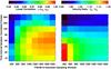 |
Fig. 9 Correlation ρ(v28,v80) (left) and mean velocity ratio v28/v80 (right) between the flow maps computed from full-resolution images (v28) and from images convolved with a Gaussian of FWHM = 160 km (v80) to match the spatial resolution of Hinode G-band images. For both cases, flow maps were computed with time cadence Δt = 10–480 s and Gaussian sampling windows with an FWHM = 400–1800 km, shown here as 8 × 8 square blocks. |
Apart from the distributions, we calculated median vmed, mean  , 10th percentile v10, and the standard deviation σv of the speed. The first three values are depicted in each panel as solid, long-dashed, and dash-dotted vertical lines, respectively. All the values describing the frequency distribution are significantly higher than the ones displayed in Fig. 7, because they were obtained from individual flow maps and not the one-hour averaged data. The first and second moments of the distributions follow the trend already discussed above for Fig. 7. A high-velocity tail (parametrized by v10) and a positive skewness is found for all distributions, likewise is always larger than vmed.
Each frequency distribution is comprised of more than 25 million flow vectors and no smoothing was applied. Thus, not only their overall shape but also the minute detail is significant. Small ripples become visible around the maximum of the distributions for Δt = 480 s and an FWHM ≥ 1200 km, suggesting that the initial feature has evolved and is no longer tracked, or other features are tracked instead. Furthermore at Δt = 480 s, the high-velocity tail has vanished in all distributions, most prominently for shorter time cadences. Another interesting feature is the shoulder at the high-velocity side of the distributions for short time cadences and narrow sampling windows, which hints at a contribution from smaller features with higher velocities. Exploding or fragmenting granules and bright points, thus, might have a different velocity spectrum distinguishing them from regular granules. In summary, Figs. 7 and 8 can also be taken as a point of reference for many other LCT studies with various input parameters, hopefully providing a more cohesive description of horizontal proper motions in the photosphere and chromosphere, or where ever time series of images are available.
As a corollary to the above parameter study, we repeated the LCT measurements but now with smoothed simulation data (Gaussian kernel with an FWHM = 160 km) to have the same spatial resolution (image scale of 80 km pixel-1) as Hinode G-band images. In Fig. 9, we use the linear correlation coefficient ρ(v28, v80) and the ratio of the velocities v28/v80 for both image scales to quantify how a coarser spatial resolution affects the flow maps. The correlation coefficients are lowest for narrow sampling windows (FWHM = 400 km) and long time cadences Δt ≥ 240 s because much of the fine structure (with high velocities) has been blurred. The highest correlations are found for FWHM ≥ 1200 km and Δt = 20–90 s. Only a very small deviation of less than 0.001 from a perfect correlation is observed for the LCT input parameters chosen in Verma & Denker (2011).
The right panel in Fig. 9 demonstrates that flow speeds could be underestimated by as much as 20% in the case of G-band images (neglecting so far the comparison with the plasma velocities in Sect. 4.5). However, such strong deviations are only observed for very narrow sampling windows and very short time cadences. In general, the speeds in both cases differ by less than 5%. Interestingly, if the time cadence is long, then there are not many traceable features left in the sampling window, but by additional smoothing, more coherent features are created that are long-lived, which explains the slightly higher velocities v80 for G-band images in the Δt = 240–400 s range. Considering that HMI continuum images have an image scale of about 360 km pixel-1 and a cadence of Δt = 45 s, broad sampling windows (FWHM ≥ 1600 km) might be needed to build up a reliable cross-correlation signal. Even though the flow speeds might be underestimated by 10–20% as compared to high-resolution simulation data (see Figs. 7 and 8), the overall morphology of the flow field will still be reliably recovered with correlation coefficients close to unity (see left panel of Fig. 9). This was also demonstrated by Beauregard et al. (2012) for complex flows along the magnetic neutral line of active region NOAA 11158 at the time of an X2.2 flare.
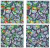 |
Fig. 10 Temporal evolution of flow fields for different time intervals between successive images and sampling window sizes: Δt = 20 s and FWHM = 600 km (left) and Δt = 60 s and FWHM = 1200 km (right). The time stamp in the lower right corner indicates the time elapsed since the beginning of the time series. The original flow maps were derived from just one pair of correlated images per time step. These maps with 273 × 273 pixels were then resampled to 50 × 50 pixels before applying a sliding average over the leading and trailing four flow maps. Speed and direction of the horizontal proper motions are given by rainbow-colored arrows (dark blue corresponds to speeds lower than 0.2 km s-1 and red to larger than 2.0 km s-1), which were superposed on the corresponding gray-scale intensity images of the CO5BOLD simulation. Major tickmarks are separated by 2 Mm. The time-dependent LCT flow fields are shown in Movie 1, which is provided in the electronic edition. |
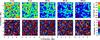 |
Fig. 11 Speed (top) and divergence (bottom) maps averaged over time intervals of ΔT = 15–120 min of the horizontal plasma velocities corresponding to an optical depth of log τ = 0. The speed and divergence values are larger roughly by a factor of three as compared to Fig. 3. |
4.4. Dynamics of horizontal proper motions
Besides quantifying persistent flow fields, LCT techniques can also capture the dynamics of horizontal proper motions. In Fig. 10, we compare snapshots from two movies with two different sets of LCT input parameters: Δt = 20 s and FWHM = 600 km (left column) and Δt = 60 s and FWHM = 1200 km (right column). The snapshots are separated by 360 s in time and show the continuum intensity with a 50 × 50 grid of superposed, color-coded flow vectors. The flow maps were smoothed both in space (5 × 5-pixel neighborhood) and time (sliding average of nine individual flow maps). These values were chosen such that watching the movies leaves a smooth and continuous visual impression. Less smoothing will result in jittering arrows in some places. We counterpoint the narrow sampling window/high cadence case with our typical choice of LCT input parameters. In the first case, much higher flow speeds are apparent, and the flow vectors in regions with high flow speeds show indications of vortex or twisting motions, which are absent in the latter case, where the flow vectors are more uniformly arranged. Comparing the flow fields at 0 s and 360 s clearly demonstrates that periods with many strong flow kernels are followed by much quieter flow fields. The high flow speeds have their origin in the borders of rapidly expanding or fragmenting granules.
4.5. Comparison with plasma velocities
The actual plasma velocities are given for three optical depths log τ = −1, 0, and +1. The time dependence of the average flow field along with the corresponding divergence maps are depicted in Fig. 11 for plasma velocities at a depth of log τ = 0. Both speed and divergence values are higher by a factor of two to three as compared to the maps in Fig. 3. The highest factor between average LCT and plasma velocities is encountered for shorter time averages. For averaging times of ΔT = 15–30 min, the speed maps exhibit more fast-moving, small-scale features associated with the boundaries of expanding or fragmenting granules. Increasing the averaging time results in smoother speed maps with much reduced speed values. By visually comparing Figs. 3 and 11, it becomes apparent that significant spatial smoothing has to be applied to the speed and divergence maps of the plasma velocities. This is a direct consequence of the sampling windows employed in LCT.
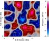 |
Fig. 12 LCT divergence map computed for input parameters: image scale 80 km pixel-1, time cadence Δt = 60 s, Gaussian sampling window with an FWHM = 1200 km, and averaging time ΔT = 1 h. Overplotted are the contours of the corresponding one-hour averaged divergence of the actual flow velocity smoothed by a Gaussian with an FWHM = 1266 km. Orange (solid) and blue (dashed) lines indicate positive and negative (± 1, ± 2 and ± 3 × 10⁻³ s-1) divergence, respectively. |
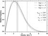 |
Fig. 13 Relative frequency distributions for the horizontal plasma velocities corresponding to different optical depths of log τ = −1, 0, and +1, which are depicted as long-dashed, dashed, and dash-dotted curves, respectively. The three vertical lines mark the position of median vmed (solid), mean |

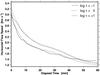 |
Fig. 14 Average horizontal flow speeds as a function of the elapsed time for the horizontal plasma velocities corresponding to optical depths of log τ = −1, 0, and +1 are depicted as long-dashed, dashed, and dash-dotted curves, respectively. The solid curve, as in Fig. 13, has to be multiplied by a factor of three to match the profile for log τ = +1. |
Figure 12 shows the divergence map for LCT flow fields computed for a one-hour time series of images, which were smoothed to match the spatial resolution of Hinode G-band images, a time cadence of Δt = 60 s, and a Gaussian sampling window with an FWHM = 1200 km. We overplotted the divergence of the actual flow velocity from an optical depth of log τ = 0 averaged over one hour and smoothed it with a Gaussian kernel with an FWHM = 1266 km. The size of the smoothing kernel was chosen such that linear correlation between the LCT and plasma maps was maximized (ρ = 0.90). The position of positive and negative divergence corresponding to the plasma flows roughly matches with the LCT divergence extrema. Even though the correlation between LCT and plasma divergence maps is significant (once properly smoothed), there are still morphological differences, not to mention the drastic difference in the absolute values of speed and divergence. In general, our findings are in good agreement with Matloch et al. (2010), e.g., their Fig. 2. In Fig. 9, we found a negligible dependence of the LCT results on the image scale (28 vs. 80 km pixel-1) or in this context equivalently the spatial resolution. Hence, for the further discussion, we use G-band-type LCT flow maps.
The frequency distributions of the actual plasma velocities are shown in Fig. 13. The distributions are assembled from the 180 velocity maps covering about one-hour. The mode of the distributions is shifted to higher velocities for higher atmospheric layers. For comparison, we show the LCT-based velocity distribution. The LCT input parameters were a time cadence of Δt = 60 s and a Gaussian sampling window with an FWHM = 1200 km. Similar to Fig. 8, the flow speeds were derived from the individual flow maps, i.e., the flow vectors were not averaged before computing the frequency distributions. We scaled the LCT frequency distribution by the factor of ≈3.01 in velocity to match it with the distributions for the actual plasma velocities. The stretched LCT and actual velocity distributions have very similar shapes. For an optical depth of log τ = 0, it had the lowest χ2-error. However, the differences in the χ2-error for all three optical depths are not significant.
In Fig. 14, we plotted the mean flow speed as a function of elapsed time for the actual plasma velocities at optical depths τ = −1, 0, and +1. We overplotted the same relation for the LCT-computed flow speed. This curve was scaled by a factor of ≈2.85 to match it with the curve for optical depth log τ = +1 as it had the lowest χ2-error. The profiles for plasma and scaled LCT velocities are very similar up to about 40 min, then the LCT velocities level out at higher velocities, which can be attributed to accumulating numerical errors of the LCT algorithm but also to small drifts over time of the intensity images. However, the fact that the curves track each other for the first 40 min is a strong indicator that LCT reliably detects the time-dependence of the actual plasma flows. Although the differences in the χ2-error are of the same order of magnitude for all three optical depths, the lower χ2-error at an optical depth of log τ = +1 indicates that LCT is picking up velocities at deeper layers in the photosphere.
Matloch et al. (2010) used the same Gaussian kernel for smoothing the plasma flows as they used for computing the LCT flow maps. In principle, this is a free parameter, which can be varied to determine how much smoothing is required to get the highest correlations between plasma and LCT flow maps. We smoothed the one-hour averaged actual flow speed vsm and divergence maps with a Gaussian kernel of size 64 × 64 pixels and with varying FWHM = 100–1500 km. We correlated it with the one-hour averaged LCT speed v80 and divergence maps for time cadences Δt = 10–480 s and Gaussian sampling windows with an FWHM = 400–1800 km. We performed this smoothing-correlation evaluation for plasma speeds at all three optical depths. However, only the results for the speed corresponding to optical depth log τ = +1 and the corresponding FWHM of the Gaussian smoothing kernel are shown in Fig. 15. The top rows for both correlation coefficient and FWHM are empty because we found no meaningful correlation between LCT maps computed with a time cadence of Δt = 480 s and the smoothed plasma flow maps. One can notice this lack of correlation already in the row for the time cadence Δt = 240 s, which shows a different behavior as compared to the remaining rows. This strongly substantiates earlier results indicating that time cadences in excess of 4 min are too long to deliver meaningful LCT results in the case of photospheric continuum images.
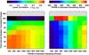 |
Fig. 15 Maximum correlation ρ(vsm,v80) (left) and corresponding FWHM of Gaussian kernel (right) used to smooth the actual flow map vsm. For both cases, the maps were averaged over one hour. The LCT flow maps were computed for images with an image-scale of 80 km pixel-1 matching Hinode G-band images, using time cadences of Δt = 10−480 s and Gaussian sampling windows with an FWHM = 400−1800 km, shown here as 8 × 8 square blocks. Gray blocks indicate parameters, where the linear correlation did not deliver meaningful results. |
The mean correlations  between the smoothed plasma vsm and LCT v80 velocities are 0.25, 0.41, and 0.49 at optical depths of log τ = −1, 0, and +1, respectively. The highest correlations are found at log τ = +1 indicating that LCT speed correlates better with plasma flows emerging from deeper layer irrespective of the LCT input parameters. Speed maps show the best correlations for smaller time cadences and narrow sampling windows. The actual plasma velocities were smoothed with kernels that are in general narrower than the LCT sampling windows (the only exception arises for the smallest FWHM = 400 km).
The divergence maps again match best with flows from deeper layers. However, the FWHM of the Gaussian kernels are about twice the size of kernels used for speed maps. At the moment, we do not have a physical interpretation why much stronger smoothing has to be applied to the plasma divergence.
All our previous findings and the difficulties in interpreting LCT flow and divergence maps have their origin in the instantaneous flow field (as already pointed out by Rieutord et al. 2001). In the left panel of Fig. 16, the local CO5BOLD plasma velocities (log τ = +1) are superposed as color-coded arrows on top of the first continuum image in the time series. Only minor spatial smoothing over a 5 × 5-pixel neighborhood was applied. The strongest horizontal flows are encountered near the boundaries of the expanding and fragmenting granules. The center of granules is almost always a divergence center and the velocity at these locations is significantly reduced. The visual appearance of this flow map is quite different from what is found in the LCT analysis. In the right panel of Fig. 16, we smoothed the CO5BOLD plasma velocities using a Gaussian kernel with an FWHM = 686 km, which produced the highest linear correlation ρ ≈ 0.57 for the time cadence Δt = 60 s and a Gaussian sampling window with an FWHM = 1200 km. As a result, velocity vectors reflecting different plasma properties (high/low speeds and convergent/divergent motions) become intermingled. The final flow map is additionally modulated by the morphology of the granular cells, which are included in the sampling window. Even by using narrower sampling windows and higher time cadences it is doubtful that the original plasma velocities can be recovered, once having been scrambled in the LCT algorithm. On the other hand, any average property of the plasma flows, which does not depend on the spatial location should remain unaffected (see Figs. 13 and 14).
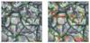 |
Fig. 16 First gray-scale intensity image of the time series overplotted with the actual (left) and smoothed CO5BOLD plasma velocity vectors at log τ = +1 (see left most panel in Fig. 10 for the corresponding LCT flow vectors). The flow field was smoothed using a Gaussian kernel with an FWHM = 686 km (see Fig. 15) corresponding to the maximum correlation coefficient between plasma and LCT (time cadence Δt = 60 s and Gaussian sampling window with an FWHM = 1200 km) velocities. The speed and direction of the flow field are given by rainbow-colored arrows, where dark blue corresponds to low and red to high velocities within the range of 0.75–7.5 km s-1 and 0.3–3.0 km s-1 for the actual and smoothed flow fields, respectively. The time-dependent CO5BOLD flow fields are shown in Movie 2, which is provided in the electronic edition. |
5. Conclusions
Applying LCT techniques to simulated data of solar granulation has proven as an excellent diagnostic to evaluate the performance of the algorithm. By contrasting LCT velocities with the plasma velocities of the simulation, some of the inherent troubles with optical flow techniques became apparent. Based on the previous analysis, we draw the following conclusions: (1) One-hour averaged LCT flow and divergence maps differ significantly, if separated by more than one hour in time. As expected, the simulation of granulation does not contain any systematic persistent flow features. However, some strong flow kernels might still survive the averaging process but they can still be of intermittent nature. (2) The time over which individual flow maps are averaged critically determines if the LCT flow field reflects either instantaneous proper motions by individual granules or longer lasting flow features. The functional dependence of the mean flow speed on the elapsed time indicates that an averaging time of at least 20 min (several times the life time of a granule) is needed to raise persistent flows to the state of being significant. (3) Time cadences Δt = 240–480 s are not suitable for tracking photospheric continuum images because the features (granules) in the tracking window have either evolved too much or moved outside the sampling window so that the cross-correlations become meaningless. (4) Smaller sampling windows track fast-moving fine structures, if high-cadence images are available, but lack the ability to measure horizontal proper motions of coherent features, which results in an underestimation of the flow speed. However, the morphology of the flow field is recovered better with narrower sampling windows. (5) Frequency distributions of flow speeds for short time cadences and narrow sampling windows indicate that exploding or fragmenting granules and bright points have a different velocity spectrum distinguishing them from regular granules. (6) LCT yields the highest speed values for sampling windows with an FWHM = 800–1000 km and short time cadences Δt = 20–30 s. (7) The input parameters time cadence Δt = 60 s, Gaussian sampling window with an FWHM = 1200 km, and averaging time ΔT = 1 h are the most reasonable choice for bulk-processing of Hinode G-band images. (8) Both the stochastic nature of granulation and the choice of LCT input parameters might be responsible for the often conflicting values in literature concerning flow speed, divergence, and vorticity. (9) Significant smoothing has to be applied to the actual plasma velocities to match the LCT flow and divergence maps. The typical velocity pattern – high velocities at the border and low speeds in the center of granules – will however be lost in the smoothing process. Thus, even with very narrow sampling windows, short time cadences, and images free of aberrations and distortions, recovering details of the plasma flows might proof a futile undertaking. (10) The LCT speeds are underestimated by a factor of three as is evident from the LCT frequency distributions (Fig. 13) and the curve for the mean LCT flow speed (Fig. 14). This scaling factor does not mean that LCT speeds can simply be multiplied by it, rather it serves as a reminder that flow fields derived from LCT have to be interpreted with caution: spatial smoothing has to be carefully considered and deriving flow velocities from intensity images will not always reflect the underlying plasma velocities.
Although the current study focuses only on granulation, in principle a similar study could be performed based on simulated data of active regions. Realistic MHD simulations of sunspots (e.g., Rempel et al. 2009; Cheung et al. 2010) could provide the basis for such a study, which will potentially aid in the interpretation of persistent flow features such as the divergence line in the mid-penumbra (e.g., Denker 1998) or the distinct flow channels of moving magnetic features connecting the sunspot’s penumbra to the surrounding supergranular cell boundary (Verma et al. 2012).
Online material
Movie of Fig. 10 Access Supplementary Material
Movie of Fig. 16 Access Supplementary Material
Acknowledgments
M.V. expresses her gratitude for the generous financial support by the German Academic Exchange Service (DAAD) in the form of a Ph.D. scholarship. C.D. was supported by grant DE 787/3-1 of the German Science Foundation (DFG).
References
- Beauregard, L., Verma, M., & Denker, C. 2012, AN, 333 [Google Scholar]
- Chae, J., & Sakurai, T. 2008, ApJ, 689, 593 [NASA ADS] [CrossRef] [Google Scholar]
- Cheung, M. C. M., Rempel, M., Title, A. M., & Schüssler, M. 2010, ApJ, 720, 233 [NASA ADS] [CrossRef] [Google Scholar]
- Denker, C. 1998, Sol. Phys., 180, 81 [NASA ADS] [CrossRef] [Google Scholar]
- Freytag, B., Steffen, M., Ludwig, H.-G., et al. 2012, J. Comp. Phy., 231, 919 [Google Scholar]
- Kosugi, T., Matsuzaki, K., Sakao, T., et al. 2007, Sol. Phys., 243, 3 [NASA ADS] [CrossRef] [Google Scholar]
- Kusano, K., Maeshiro, T., Yokoyama, T., & Sakurai, T. 2002, ApJ, 577, 501 [NASA ADS] [CrossRef] [Google Scholar]
- Lantz, S. R., & Fan, Y. 1999, ApJS, 121, 247 [Google Scholar]
- Leese, J. A., Novak, C. S., & Clark, B. B. 1971, J. Appl. Meteor., 10, 118 [NASA ADS] [CrossRef] [Google Scholar]
- Longcope, D. W. 2004, ApJ, 612, 1181 [Google Scholar]
- Matloch, Ł., Cameron, R., Shelyag, S., Schmitt, D., & Schüssler, M. 2010, A&A, 519, A52 [NASA ADS] [CrossRef] [EDP Sciences] [Google Scholar]
- Muller, R., Auffret, H., Roudier, T., et al. 1992, Nature, 356, 322 [NASA ADS] [CrossRef] [Google Scholar]
- November, L. J., & Simon, G. W. 1988, ApJ, 333, 427 [Google Scholar]
- Pesnell, W. D., Thompson, B. J., & Chamberlin, P. C. 2012, SoPh, 275, 3 [NASA ADS] [Google Scholar]
- Rempel, M., Schüssler, M., Cameron, R. H., & Knölker, M. 2009, Science, 325, 171 [NASA ADS] [CrossRef] [PubMed] [Google Scholar]
- Rieutord, M., Roudier, T., Ludwig, H.-G., Nordlund, Å., & Stein, R. 2001, A&A, 377, L14 [NASA ADS] [CrossRef] [EDP Sciences] [Google Scholar]
- Scherrer, P. H., Schou, J., Bush, R. I., et al. 2012, SoPh, 275, 207 [Google Scholar]
- Schuck, P. W. 2005, ApJ, 632, L53 [NASA ADS] [CrossRef] [Google Scholar]
- Schuck, P. W. 2006, ApJ, 646, 1358 [NASA ADS] [CrossRef] [Google Scholar]
- Tsuneta, S., Ichimoto, K., Katsukawa, Y., et al. 2008, SoPh, 249, 167 [Google Scholar]
- Verma, M., & Denker, C. 2011, A&A, 529, A153 [NASA ADS] [CrossRef] [EDP Sciences] [Google Scholar]
- Verma, M., Balthasar, H., Deng, N., et al. 2012, A&A, 538, A109 [NASA ADS] [CrossRef] [EDP Sciences] [Google Scholar]
- Vögler, A., Shelyag, S., Schüssler, M., et al. 2005, A&A, 429, 335 [NASA ADS] [CrossRef] [EDP Sciences] [Google Scholar]
- Wedemeyer-Böhm, S., & Rouppe van der Voort, L. 2009, A&A, 503, 225 [NASA ADS] [CrossRef] [EDP Sciences] [Google Scholar]
- Welsch, B. T., Fisher, G. H., Abbett, W. P., & Regnier, S. 2004, ApJ, 610, 1148 [NASA ADS] [CrossRef] [Google Scholar]
- Welsch, B. T., Abbett, W. P., De Rosa, M. L., et al. 2007, ApJ, 670, 1434 [NASA ADS] [CrossRef] [Google Scholar]
All Figures
|
Fig. 1 First (left) and one-hour averaged (right) images with 400 × 400 pixels and an image scale of 28 km pixel-1 taken from a CO5BOLD time series of solar granulation. Because of the Gaussian kernels (in the insert lower right corner) of 128 × 128 pixels used as sampling windows, the original image size was reduced by 128 pixels. The white squares mark the region with a size of 273 × 273 pixels that remains after the LCT computation. |
| In the text | |
|
Fig. 2 Average speed (top) and divergence (bottom) maps for the first (left) and last (right) hour of the time series computed using a time cadence of Δt = 60 s and a Gaussian sampling window with an FWHM = 1200 km. The direction and magnitude of the horizontal flows are plotted over the divergence maps as arrows, for which a velocity of 0.5 km s-1 corresponds to exactly the grid spacing. The values displayed at the top are the mean speed |
| In the text | |
|
Fig. 3 Speed (top) and divergence (bottom) maps averaged over time intervals of ΔT = 15–120 min. The LCT maps were computed using a time cadence of Δt = 60 s and a Gaussian sampling window with an FWHM = 1200 km. |
| In the text | |
|
Fig. 4 Average horizontal flow speed as a function of the elapsed time. The maps were computed using a Gaussian sampling window with an FWHM = 1200 km and time cadence Δt = 60 s. Before computing the cross-correlations, the images were convolved with a Gaussian kernel FWHM = 40–320 km to degrade the spatial resolution of the images. The increasing FWHM values are presented as progressively lighter shades of gray. The dash-dotted and dashed lines represents values above and below optimal parameter (FWHM = 160 km), respectively. The black solid line is used to depict result for the FWHM = 160 km, which is the typical spatial resolution of most Hinode G-band images (see Verma & Denker 2011). |
| In the text | |
|
Fig. 5 Average horizontal flow speed as a function of the elapsed time. The maps were computed using a Gaussian sampling window with an FWHM = 1200 km and time cadence Δt = 10–480 s. The increasing time cadences Δt are presented as progressively lighter shades of gray. The black solid line is depicting the result for the time cadence Δt = 60 s, which has been identified in Verma & Denker (2011) as an optimal choice for tracking horizontal proper motions in Hinode G-band time-series data. |
| In the text | |
|
Fig. 6 Average horizontal flow speed as a function of the elapsed time. The maps were computed using a time cadence Δt = 60 s and Gaussian sampling window with various FWHM = 400–1800 km. The increasing FWHM values are presented as progressively lighter shades of gray. The black solid line is used to depict the result for a Gaussian sampling window with an FWHM = 1200 km, which has been identified in Verma & Denker (2011) as an optimal choice for tracking horizontal proper motions in Hinode G-band time-series data. |
| In the text | |
|
Fig. 7 Horizontal flow speed maps (one-hour averages) computed with time cadences Δt = 10–480 s (bottom to top) and Gaussian kernels with an FWHM = 400–1800 km (left to right). Displayed at the top of the panels are the mean speed |
| In the text | |
|
Fig. 8 Relative frequency distributions of horizontal flow speeds computed with time cadences Δt = 10–480 s (bottom to top) and Gaussian sampling windows with an FWHM = 400–1800 km (left to right). The three vertical lines mark the position of median vmed (solid), mean |
| In the text | |
|
Fig. 9 Correlation ρ(v28,v80) (left) and mean velocity ratio v28/v80 (right) between the flow maps computed from full-resolution images (v28) and from images convolved with a Gaussian of FWHM = 160 km (v80) to match the spatial resolution of Hinode G-band images. For both cases, flow maps were computed with time cadence Δt = 10–480 s and Gaussian sampling windows with an FWHM = 400–1800 km, shown here as 8 × 8 square blocks. |
| In the text | |
|
Fig. 10 Temporal evolution of flow fields for different time intervals between successive images and sampling window sizes: Δt = 20 s and FWHM = 600 km (left) and Δt = 60 s and FWHM = 1200 km (right). The time stamp in the lower right corner indicates the time elapsed since the beginning of the time series. The original flow maps were derived from just one pair of correlated images per time step. These maps with 273 × 273 pixels were then resampled to 50 × 50 pixels before applying a sliding average over the leading and trailing four flow maps. Speed and direction of the horizontal proper motions are given by rainbow-colored arrows (dark blue corresponds to speeds lower than 0.2 km s-1 and red to larger than 2.0 km s-1), which were superposed on the corresponding gray-scale intensity images of the CO5BOLD simulation. Major tickmarks are separated by 2 Mm. The time-dependent LCT flow fields are shown in Movie 1, which is provided in the electronic edition. |
| In the text | |
|
Fig. 11 Speed (top) and divergence (bottom) maps averaged over time intervals of ΔT = 15–120 min of the horizontal plasma velocities corresponding to an optical depth of log τ = 0. The speed and divergence values are larger roughly by a factor of three as compared to Fig. 3. |
| In the text | |
|
Fig. 12 LCT divergence map computed for input parameters: image scale 80 km pixel-1, time cadence Δt = 60 s, Gaussian sampling window with an FWHM = 1200 km, and averaging time ΔT = 1 h. Overplotted are the contours of the corresponding one-hour averaged divergence of the actual flow velocity smoothed by a Gaussian with an FWHM = 1266 km. Orange (solid) and blue (dashed) lines indicate positive and negative (± 1, ± 2 and ± 3 × 10⁻³ s-1) divergence, respectively. |
| In the text | |
|
Fig. 13 Relative frequency distributions for the horizontal plasma velocities corresponding to different optical depths of log τ = −1, 0, and +1, which are depicted as long-dashed, dashed, and dash-dotted curves, respectively. The three vertical lines mark the position of median vmed (solid), mean |
| In the text | |
|
Fig. 14 Average horizontal flow speeds as a function of the elapsed time for the horizontal plasma velocities corresponding to optical depths of log τ = −1, 0, and +1 are depicted as long-dashed, dashed, and dash-dotted curves, respectively. The solid curve, as in Fig. 13, has to be multiplied by a factor of three to match the profile for log τ = +1. |
| In the text | |
|
Fig. 15 Maximum correlation ρ(vsm,v80) (left) and corresponding FWHM of Gaussian kernel (right) used to smooth the actual flow map vsm. For both cases, the maps were averaged over one hour. The LCT flow maps were computed for images with an image-scale of 80 km pixel-1 matching Hinode G-band images, using time cadences of Δt = 10−480 s and Gaussian sampling windows with an FWHM = 400−1800 km, shown here as 8 × 8 square blocks. Gray blocks indicate parameters, where the linear correlation did not deliver meaningful results. |
| In the text | |
|
Fig. 16 First gray-scale intensity image of the time series overplotted with the actual (left) and smoothed CO5BOLD plasma velocity vectors at log τ = +1 (see left most panel in Fig. 10 for the corresponding LCT flow vectors). The flow field was smoothed using a Gaussian kernel with an FWHM = 686 km (see Fig. 15) corresponding to the maximum correlation coefficient between plasma and LCT (time cadence Δt = 60 s and Gaussian sampling window with an FWHM = 1200 km) velocities. The speed and direction of the flow field are given by rainbow-colored arrows, where dark blue corresponds to low and red to high velocities within the range of 0.75–7.5 km s-1 and 0.3–3.0 km s-1 for the actual and smoothed flow fields, respectively. The time-dependent CO5BOLD flow fields are shown in Movie 2, which is provided in the electronic edition. |
| In the text | |
Current usage metrics show cumulative count of Article Views (full-text article views including HTML views, PDF and ePub downloads, according to the available data) and Abstracts Views on Vision4Press platform.
Data correspond to usage on the plateform after 2015. The current usage metrics is available 48-96 hours after online publication and is updated daily on week days.
Initial download of the metrics may take a while.