| Issue |
A&A
Volume 548, December 2012
|
|
|---|---|---|
| Article Number | A91 | |
| Number of page(s) | 23 | |
| Section | Interstellar and circumstellar matter | |
| DOI | https://doi.org/10.1051/0004-6361/201218859 | |
| Published online | 28 November 2012 | |
Physical conditions in the gas phases of the giant H II region LMC-N 11 unveiled by Herschel
I. Diffuse [C II] and [O III] emission in LMC-N 11B⋆,⋆⋆
1
Laboratoire AIM, CEA/DSM-CNRS-Université Paris Diderot DAPNIA/Service
d’Astrophysique, Bât. 709, CEA-Saclay,
91191
Gif-sur-Yvette Cedex,
France
e-mail: vianney.lebouteiller@cea.fr
2
Department of Astronomy, University of Virginia,
PO Box 3818, Charlottesville, VA
22903,
USA
3
Department of Physics, University of Cincinnati,
Cincinnati, OH
45221,
USA
4
Max-Planck-Institute for Extraterrestrial Physics
(MPE), Giessenbachstraße
1, 85748
Garching,
Germany
Received: 20 January 2012
Accepted: 26 September 2012
Context. The Magellanic Clouds provide a nearby laboratory for metal-poor dwarf galaxies. The low dust abundance enhances the penetration of UV photons into the interstellar medium (ISM), resulting in a relatively larger filling factor of the ionized gas. Furthermore, there is very likely a molecular gas reservoir probed by the [C ii] 157 μm line not traced by CO(1–0), the so-called “dark” gas. The Herschel Space Telescope allows us to observe far-infrared (FIR) cooling lines and to examine the physical conditions in the gas phases of a low-metallicity environment to unprecedented, small spatial scales.
Aims. Our objective is to interpret the origin of the diffuse emission of FIR cooling lines in the H ii region N 11B in the Large Magellanic Cloud. We first investigate the filling factor of the ionized gas. We then constrain the origin of the [C ii] line by comparing to tracers of the low-excitation ionized gas and of photodissociation regions (PDRs).
Methods. We present Herschel/PACS maps of N 11B in several tracers, [C ii] 157 μm, [O i] 63 μm and 145 μm, [N ii] 122 μm, [N iii] 57 μm, and [O iii] 88 μm. Optical images in Hα and [O iii] 5007 Å were used as complementary data to investigate the effect of dust extinction. Observations were interpreted with photoionization models to infer the gas conditions and estimate the ionized gas contribution to the [C ii] emission. PDRs were probed through polycyclic aromatic hydrocarbons (PAHs) observed with the Spitzer Space Telescope.
Results. [O iii] 88 μm is dominated by extended emission from the high-excitation diffuse ionized gas. This is the brightest FIR line throughout N 11B, ~4 times brighter than [C ii]. We find that about half of the emission from the ionized gas is extinguished by dust. We modeled [O iii] around each O-type star and find that the density of the ISM is ≲16 cm-3 on large scales. The extent of the [O iii] emission suggests that the medium is rather fragmented, allowing far-UV photons to permeates the ISM to scales of ≳30 pc. Furthermore, by comparing [C ii] with [N ii] 122 μm, we find that 95% of [C ii] arises in PDRs, except toward the stellar cluster for which as much as 15% could arise in the ionized gas. We find a remarkable correlation between [C ii]+[O i] and PAH emission, with [C ii] dominating the cooling in diffuse PDRs and [O i] dominating in the densest PDRs. The combination of [C ii] and [O i] provides a proxy for the total gas cooling. Our results suggest that PAH emission describes better the gas heating in PDRs as compared to the total infrared emission.
Key words: infrared: ISM / HII regions / ISM: lines and bands / dust, extinction / methods: data analysis
Herschel is an ESA space observatory with science instruments provided by European-led Principal Investigator consortia and with important participation from NASA.
Appendix A is available in electronic form at http://www.aanda.org
© ESO, 2012
1. Introduction
Dwarf galaxies are important testbeds for understanding star formation in metal-poor environments that are intermediate between primordial galaxies and evolved systems such as the Milky Way. The low dust abundance in a metal-poor interstellar medium (ISM) allows far-ultraviolet (FUV) photons to permeate on larger physical scales in interstellar clouds. This effect reduces the size of the CO cores and pushes the C+/C0/CO interface deeper into the cloud, hence the very low CO luminosities (e.g., Leroy et al. 2006) and the difficulty of accurately determining the molecular hydrogen reservoir. Since molecular hydrogen (H2) is more efficiently self-shielded from photodissociation than is CO, this potentially results in a thick layer where H2 exists along with C+ and C0 (Grenier et al. 2005; Roellig et al. 2006; Wolfire et al. 2010). This so-called “dark gas” might represent a significant fraction of the molecular mass in metal-poor galaxies (Madden et al. 1997).
Main parameters of the transitions used in this study.
The ratio of the far-infrared (FIR) line [C ii] 157 μm to CO(1–0) is found to be much higher in dwarf galaxies than in normal galaxies (Madden et al. 1997; Pineda et al. 2008), hinting at a possibly significant dark gas reservoir. However, many uncertainties remain regarding the exact origin of the [C ii] line as a function of star-formation activity and metallicity. Given the ionization potential of C0 (11.3 eV) and the low excitation temperature of the 157 μm line (91 K), [C ii] can originate in the cold and warm neutral atomic and molecular medium and in the warm ionized gas (see also Madden et al. 1993; Heiles 1994). These phases coexist in a single beam for most extragalactic observations, complicating the diagnostics drawn from [C ii]. It is therefore essential to probe the smallest physical scale possible in the closest galaxies in order to constrain the conditions of [C ii] emission. This has proven to be a challenge until now, especially for dwarf galaxies.
The relatively larger mean free path of FUV photons in low-metallicity environments also results in a large filling factor of ionized gas. The best probe for estimating this filling factor is an optically thin tracer with a low critical density (i.e., the density for which the spontaneous radiation rate equals the collision rate) and an ionization potential permitting its presence outside the dense H ii regions. [O iii] 88 μm, [N ii] 122 μm, and [N ii] 205 μm are the best probes available (see critical densities and ionization potentials in Table 1).
The PACS instrument (Poglitsch et al. 2010) on board the Herschel Space Telescope (Pillbratt et al. 2010) observes with a spatial resolution of ~10–13″, which allows (1) examining the distribution of [C ii] in nearby galaxies and (2) comparing the local excitation conditions of this important coolant to those of complementary tracers of the high-excitation ionized gas ([N iii] 57 μm, [O iii] 88 μm), of the low-excitation ionized gas (e.g., [N ii] 122 μm, 205 μm), and of the neutral and molecular gas ([O i] 63 μm, 145 μm).
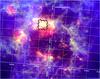 |
Fig. 1 The giant H ii region N 11, with Spitzer/MIPS 24 μm shown in red, Spitzer/IRAC 8.0 μm in green, and H i column density (from Kim et al. 2003) in blue. The Spitzer/MIPS 24 μm emission is dominated by very small grains that are stochastically heated and by big, warm, dust grains in thermal equilibrium with the interstellar radiation field. Spitzer/IRAC 8.0 μm emission is dominated by PAHs. The polygon shows the Herschel/PACS spectroscopic observations of N 11B presented in this paper. |
The Magellanic Clouds provide both a local dwarf galaxy template and a moderately metal-poor environment, with a metallicity of ≈1/2 Z⊙ for the Large Magellanic Cloud (LMC) and ≈1/5 Z⊙ for the Small Magellanic Cloud (SMC). The presence of massive star-forming regions, such as 30 Doradus and N 11 in the LMC, makes it possible to constrain the origin of [C ii] in the various phases involved in star formation. The Herschel SHINING guaranteed time key program (P.I. E. Sturm) observed several H ii regions in N 11 with PACS. The first objective is to unveil the particular morphology of the ISM in a metal-poor environment through the study of the ionized gas distribution and filling factor. The second objective is to understand and constrain the origin of the [C ii] emission in order to account for the molecular gas reservoir that is not seen in CO. In the present paper, we investigate the large-scale emission-line structures in the N 11B H ii region that is the northern and brightest H ii region in the N 11 complex (Fig. 1). In a second paper (Lebouteiller et al., in prep.), we examine the other H ii regions in the N 11 complex, with a focus on the physical conditions in the photodissociation regions (PDRs).
In Sect. 2, we describe the environment and morphology of N 11B. We present the observations in Sect. 3 and the data analysis in Sect. 4. The spatial distribution of the FIR tracers is examined in Sect. 5, and the physical conditions of the ionized gas are investigated in Sect. 6. The ionized gas spatial distribution is discussed in Sect. 7. Finally, the origin of the [C ii] emission is discussed in Sect. 8. We present the Herschel/PACS data reduction and analysis tool PACSman in the appendix.
2. Environment
2.1. Morphology
N 11 (also DEM 34; Henize 1956; Davies et al. 1976) is the second largest giant H ii region in the Large Magellanic Cloud after 30 Doradus (Kennicutt & Hodge 1986). The morphology of N 11 consists of nine distinct nebulae (N11A-N11I; Rosado et al. 1996) distributed around the OB association LH 9 (NGC 1760), which is dominated by the compact cluster HD 32228 (also Radcliffe 64, Sk-66-28, or Breysacher 9). The LH 9 association carved out a cavity and triggered a secondary, peripheral starburst (Lucke & Hodge 1970; Parker et al. 1992; Walborn & Parker 1992). The starburst shell created by LH 9 reached ~120 pc in diameter (80 × 60 pc, Lucke & Hodge 1970). Figure 1 shows the H i hole corresponding to the cavity around LH 9. The nebulae are distributed around the H i shell; N 11B is the brightest nebula to the north.
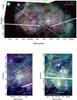 |
Fig. 2 Top − HST/ACS color-composite image of the N 11B region (blue: F814; green: F658N/Hα; red: F660N/[N ii]). Images were downloaded from the Hubble Legacy Archive (http://hla.stsci.edu/) and later stitched with Montage (http://montage.ipac.caltech.edu/). The white stripes correspond to a gap between individual exposures. The yellow polygon indicates the field-of-view of the Herschel/PACS observations ( ≈ 2.3′ × 2.3′). The 4 rectangles in color indicate specific regions discussed in the text. The dashed circles represent the ISO-LWS observation (from 65′′ to 80′′FWHM beam) and the slit represents the optical observation by Tsamis et al. (2001). Bottom − Close-up of the eastern (left panel) and western (right panel) sides. The stellar complexes are labeled as the brightest star with a “+” sign appended. |
There is evidence of ongoing star formation in N 11B. About 20 HAeBe stars, which are intermediate-mass (3 to 7 M⊙) pre-main sequence stars (1 to 3 Myr), have been detected (Barba et al. 2003; Hatano et al. 2006). A methanol maser of 0.3 Jy was observed by Ellingsen et al. (1994). Finally, Hatano et al. (2006) identified two ultracompact H ii regions, one at (04h56m48s, −66°24′34′′), corresponding to the radio source known as W2 (or B0456-6629) in Indebetouw et al. (2004), and the other at (04h56m57s − 66°25′13′′), which is known as W1 (or B0456-6629).
From the Hubble Space Telescope (HST) Advanced Camera for Surveys (ACS) archival images (Fig. 2), two regions can be distinguished within N 11B with distinct morphological attributes. The eastern half has sharp edges toward the east and the south, indicating the presence of relatively dense interfaces. A lower density zone is seen in the middle of N 11B, with the OB association PGMW 3204/09 (hereafter the “footprint” cluster; Sect. 2.2) surrounded by several small clouds with bright ionization fronts, including the kiwi-shaped cloud and the Y-shaped cloud described in Nazé et al. (2001). The western half of N 11B is dominated by PDR structures north of the local OB association LH 10. Several ionization fronts (I1, I2, and I3 in Barbá et al. 2003) are seen above LH 10.
In the following we concentrate on four distinct regions that were selected based on their extreme nature among N 11B, translating into significant differences in line ratio diagnostics:
-
the fragmented region within the orange box inFig. 2, which we refer to as W2 from now on,which contains relatively dense interfaces under the influence ofnearby massive stars from the LH 10 cluster;
-
the stellar cluster below W2, which we refer to from now on as LH 10 (red box). LH 10 is embedded in a relatively diffuse gas;
-
the northern region (green box), where the absence of optical edge or arcs suggests a smooth transition into the general, lower density, LMC environment. This region is little, if at all, affected by known massive stars;
-
the compact region W1 (blue box), which contains a small stellar cluster surrounded by dense shells.
2.2. Main ionizing sources
The stellar cluster associated with N 11B is the LH 10 OB association (also NGC 1763, IC 2115, Lucke & Hodge 1970). LH 10 is the youngest cluster in N 11 (≲3 Myr; Walborn et al. 1999). Most of the stars in LH 10 are gathered into several compact complexes located south of the W2 star-forming region. The PGMW 3128 and the PGMW 3120 complexes are located near W2, while the PGMW 3090 and PGMW 3070 are farther away to the south (Parker et al. 1992; Fig. 2). From the high-resolution HST/ACS image, we count at least 260 stars south of W2. Including faint sources increases the number to more than 300 stars. This is a lower limit since some complexes are unresolved. At least two O3 stars were identified in the southern LH 10 cluster, PGMW 3058 and PGMW 3061, slightly off the area covered by our PACS observations (Parker et al. 1992). The presence of “intact” (not yet evolved) O3 stars suggests that no supernova event has occurred yet.
The “footprint” cluster is located to the east of N 11B (see lower left panel in Fig. 2) and close to the kiwi-shaped cloud, with several massive stars and concentrations identified by Parker et al. (1992). The main sources are PGMW 3204-3209-3211, with at least 30 stars (Fig. 2). An O3 III star was discovered in PGMW 3209 (star “A” in Walborn & Parker 1992). Another concentration is located nearby, to the east of the Y-shaped cloud with at least a dozen stars.
2.3. Electron density
Mac Low et al. (1998) find an electron density of ne ≈ 38 cm-3 from the Hα emission measure, assuming N 11B is a uniform ionized sphere. By estimating the physical size of structures within the nebula, Nazé et al. (2001) find that the emission measure is consistent with ne ~ 15 cm-3 in the lowest surface brightness regions. It reaches 50–150 cm-3 in moderately bright arcs and up to 200–500 cm-3 in the bright ridges of dust clouds (e.g., the kiwi-shape cloud). The bright optical arcs studied by Nazé et al. (2001) correspond to the highest densities and also show low [O iii] 5007 Å/Hα ratios, which is attributed to lower ionization and excitation.
Tsamis et al. (2001) observed the [S ii] λ6731/λ6716 and [O ii] λ3729/λ3726 doublets in long-slit spectroscopy (see slit position in Fig. 2) and find ne = 80 cm-3 and 110 cm-3, respectively. They measure a significantly higher density from the [Cl iii] λ5537/λ5517 doublet, with 1700 cm-3, which they attribute to the higher critical densities involved in the [Cl iii] transitions. Strong density variations are therefore expected in N 11B. We tentatively expect a density of ~25 cm-3 for the low-density nebula and densities between 100–1000 cm-3 for the bright optical arcs.
2.4. Chemical abundances
Chemical abundances in N 11B were derived by Tsamis et al. (2003), who find 12 + log (O/H) = 8.41 and 12 + log (N/H) = 6.93. Using the oxygen solar abundance 12 + log (O/H) = 8.69 from Asplund (2009), the metallicity is 0.52 Z⊙. The N/O abundance ratio is significantly lower than the solar value since N/H is ≈7 times below the solar abundance. This nitrogen deficiency is observed in several H ii regions of the LMC and is likely due to depletion of N on dust grains (e.g., Garnett 1999). For the carbon abundance, we assume 12 + log (C/H) = 7.9 which is the average abundance in LMC H ii regions (Garnett 1999).
3. Observations
N 11B was observed on January 4, 2010 with the PACS spectrometer on board Herschel. The main FIR fine-structure lines were mapped in the wavelength-switching mode (later decommissioned and replaced by the unchopped scan mode): [N iii] 57 μm, [O i] 63 μm, [N ii] 122 μm, [O i] 145 μm, [C ii] 157 μm, [N ii] 205 μm (OBSID 1342188940), and [O iii] 88 μm (OBSID 1342188941). Two follow-up observations were performed in unchopped scan mode, one pointing toward W2 in [N ii] 122 μm on April 4, 2011 (OBSID 1342219439), and one pointing toward W1 in [N ii] 122 μm and [O i] 145 μm on July 19, 2011 (OBSID 1342225175). The [O iii] 52 μm was not observed with PACS because of the low transmission at this wavelength, but the line was detected with ISO (Sect. 4.2). The observed lines are listed in Table 1 along with a summary of the main transition parameters. From now on we use the line notation with the wavelength as subscript for ambiguous cases (e.g., [O i]63 for [O i] 63 μm).
As explained in Poglitsch et al. (2010), the PACS spectrometer is an integral-field spectrometer that samples the spatial direction with 25 pixels and the spectral direction with 16 pixels. Each spectral pixel “sees” a distinct wavelength range that is scanned by varying the grating angle. The resulting projection of the PACS array on the sky is a footprint of 5 × 5 spatial pixels (“spaxels”), corresponding to a 47″ × 47″ field-of-view. At a distance of the LMC (48.5 kpc), the footprint size 47″ corresponds to 11 pc. The map observations of N 11B were designed as 3 × 3 raster map, with an overlap of ≈1.5 spaxels. Figure 2 shows the PACS map coverage (about 2.3′ × 2.3′) on the optical image. According to the PACS Observers Manual1, the point spread function full width at half maximum (FWHM) is ≈9.5″ (≈2.2 pc) between 55 μm and 100 μm, and it increases to about ≈13″ (≈3 pc) at 180 μm.
4. Data analysis
4.1. Herschel/PACS
The data reduction was performed in HIPE track number 4.0.700 (Ott 2010) using a combination of the default wavelength-switching and unchopped scan scripts.
4.1.1. Wavelength-switching
A spatially offset position is usually observed at the beginning and at the end of the observation to subtract the telescope background emission. In our mapping observations, the offset was located on the source itself (central raster position in the map) so that it was not subtracted but instead used to increase the signal-to-noise ratio (S/N) by ~ at that location. Based on the unchopped scan observation, for which an offset was available (Sect. 4.1.2), we estimate that the lack of an offset in the wavelength-switching observation resulted in a lower S/N in the final spectra. No line contamination from the Milky Way was observed in the offset in the unchopped scan observation, implying that our line measurements are not affected by foreground line emission, as expected from the low galactic latitude of LMC-N 11 (~− 66.4°).
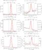 |
Fig. 3 Line fits are shown for one spaxel observing the W2 region. The histogram shows the rebinned data, the thin curve shows the continuum, and the thick curve shows the fit. The fit was performed on the data cloud, which contains ≈ 140 000 points. We show the rebinned spectrum for display purposes. |
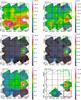 |
Fig. 4 Herschel/PACS maps (in J2000 coordinates). The colorbar gives the flux in W m-2 sr-1. The dashed rectangles correspond to the zones described in Fig. 2 and Sect. 2.1. The spatial resolution is about ≈ 9.5″ for [N iii]57, [O i]63, and [O iii]88, ≈ 11.5″ for [N ii]122, [O i]145, and [C ii]157. |
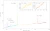 |
Fig. 5 ISO LWS spectrum of N 11B. See Fig. 2 for the location of the observation pointing. The colors correspond to the different spectral orders. The [O iii]88 is observed in 2 spectral orders with different spectral resolutions. The displayed spectrum was extracted using a point-like source calibration. |
The wavelength-switching mode was initially designed to remove the variations in the telescope background emission on small timescales by switching wavelengths rapidly, resulting in a differential spectral line profile. The wavelength modulation of the grating follows the AABBBBAA pattern, where A observes at the nominal wavelength and B observes the modulated wavelength (with a shift of about half of the FWHM).
The differential line profile resulting from the wavelength-switching proved itself difficult to fit, especially for low S/Ns. We decided to consider the line profile in the combined spectrum A+B (i.e., without subtracting the switched wavelength spectrum). This is effectively a similar approach to the unchopped scan mode. The final spectrum was divided by a factor 1.3 for the blue camera and 1.1 for the red camera in order to account for differences between ground and in-flight performances (PACS ICC calibration document PICC-KL-TN-041).
4.1.2. Unchopped scan
Follow-up pointed observations of [N ii]122 and [O i]145 were performed with the unchopped scan mode. The offset exposures were checked for line emission and were averaged before subtraction from the “on-source” observations. The unchopped scan observations took longer (per line and for one raster position) than the wavelength-switching, and transient cosmic rays were observed on the timeline of several photoconductor pixels. We corrected the signal by using a multiresolution algorithm that is part of the data reduction and analysis PACSman (see Appendix).
4.1.3. Line fitting and map projection
Line fits were performed by PACSman (see Appendix) for each spaxel at each raster position. A Gaussian profile was adjusted simultaneously with a polynomial continuum of degrees one to three. All lines have heliocentric radial velocities of 305 ± 20 km s-1 with no significant variations across the map. This velocity is consistent with the value 292 ± 23 km s-1 found by Rosado et al. (1995) for the entire N 11B nebula. The instrument spectral resolution ranges from ≈55 km s-1 to ≈320 km s-1 depending on the band/order and wavelength. No significant additional broadening is observed for the long-wavelength lines [O i]145 and [C ii], while a broadening of 70–90 km s-1 is observed for [N iii], [O i]63, and [O iii]88 (for which the spectral resolution is finer), which might be real. Example of line fits are shown in Fig. 3.
For the mapping observations, the line fluxes of all the spaxels are projected on a subpixel grid (see Appendix). The subpixel size (1/3 of the spaxel size, i.e., ≈3″ or ≈0.7 pc at the distance of the LMC) is chosen in order to recover the best possible spatial sampling in the footprint overlap regions. For comparison, the map of the Orion bar in Bernard-Salas et al. (2012) is 0.25 pc in size, i.e., a fraction of one pixel in our maps.
The S/N is >50 in the [O iii]88 line across the map, >12 in the [C ii] map, between 1 and 100 in the [O i]63 map, between 0 and 17 in the [O i]145 map, and between 0.5 and 7 in the [N iii] map. The [N ii]122 line is barely detected in a few positions, while [N ii]205 is not detected anywhere because of the known spectral leakage in the R1 band (see PACS Observers Manual). Final maps are shown in Fig. 4.
4.2. Ancillary data
N 11B was observed with the ISO space telescope (Kessler et al. 1996) in the LWS filter (45–200 μm) with a beam size between 65″ and 80″. We retrieved the archival data, extracted the spectrum (Fig. 5), and measured the line fluxes. The flux determinations are listed in Table 2. The values assuming a point-like source calibration agree within 10% with Vermeij et al. (2002)2. We also extracted the line fluxes assuming an extended source calibration. The good alignment of the dust continuum across the spectral orders in Fig. 5 suggests that the dust distribution is point-like. We compared the ISO line fluxes with the integrated fluxes derived from the PACS maps in the same aperture (Fig. 2). The PACS fluxes agree remarkably well with the ISO results. The PACS fluxes are slightly underestimated because of the incomplete coverage of the ISO beam (Fig. 2).
Line fluxes derived from the ISO LWS spectrum.
We also used the calibrated HST/WFPC2 images in the F502N and F658N narrow band filters, kindly provided to us by Nazé (see also Nazé et al. 2001). The F502N band is dominated by the [O iii] 5007 Å (hereafter [O iii]opt) line emission. The continuum emission, which is dominated by dust-scattered light in N 11B, represents only a small fraction (≲1%) of the emission within the narrow filter as compared to [O iii]opt in the long-slit used by Tsamis et al. (2008). We assumed that the continuum emission remains negligible throughout the region. A similar assumption was used for the F658N band and the Hα line. The WFPC2 images were convolved with a Gaussian PSF to reach a spatial resolution of 12″, i.e., slightly larger than the PACS resolution (≈10″). The WFPC2 images were then resampled to the PACS image pixel size (Sect. 4.1.3). The final [O iii]opt and Hα maps are shown in Fig. 6.
We derived the polycyclic aromatic hydrocarbon (PAH) emission by using the archival Spitzer/IRAC images. We used band 4, centered at 8.0 μm, which observes the PAH complex at 7.7 μm and 8.6 μm along with the warm dust continuum. To remove the warm dust contribution, we assumed a power-law emission on the Wien side of the spectral energy distribution (SED) and used the emission in bands 1 (3.6 μm) and 2 (4.5 μm) to extrapolate to the band 4 wavelength range for each pixel. The correction thereby applied is ~10%. We then calibrated the flux density in band 4 by using a template source spectrum, as explained in the Spitzer synthetic photometry cookbook3. The template spectrum was built from an incomplete Spitzer/IRS map of N 11B, covering the LH 10 and W2 regions (AORKEY 22469632). From the IRAC transmission curve, we further estimated that about ≈45% of the total PAH emission (including features from 5 μm to 18 μm) falls within band 4. We therefore corrected the PAH map by this factor. The final PAH map is presented in Fig. 6.
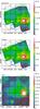 |
Fig. 6 [O iii]opt, Hα, and PAH maps, from top to bottom. The images were convolved at the resolution of the Herschel [C ii] map. See Fig. 4 for the figure description. |
5. Distribution of the FIR lines
The main observational results (noise level and integrated flux) are provided in Table 3. We discuss the detailed results for each line in the following.
Summary of observations and integrated emission properties.
5.1. [O I]
Both [O i]63 and [O i]145 have high critical densities (Table 1) and trace mostly the dense gas in PDRs. The two lines show nearly identical distributions (Fig. 4), most of the differences being due to the lower S/N of the [O i]145 map in the fainter and more diffuse regions. The [O i]145 emission is dominated by the region W2, while fainter emission is also seen toward the three compact regions on the eastern side, including the region W1.
The [O i]63 line is detected throughout the entire map, its intensity varying by a factor of ~90 (Table 3). The line ratio [O i]145/[O i]63 varies from ≈0.05 to ≈0.11 across the map. The integrated [O i]63 emission in the map is 3.9 × 10⁻¹⁴ W m-2, about ≈39% of which comes from W2, and ≈44% come from both W1 and W2. This fraction is remarkably large as compared to the area covered by W1+W2 within the PACS map (~13%).
5.2. [C II]
The [C ii] line is thought to be the dominant cooling mechanism in low-density PDRs and in the diffuse ISM for temperatures ≲8 × 10³ K (Dalgarno & McCray 1972; Tielens & Hollenbach 1985a,b; Wolfire et al. 1995). Depending on the ionization fraction of the gas, excitation of the 2P3/2 level is due to inelastic collisions with neutral hydrogen atoms and molecules or with electrons (Dalgarno & McCray 1972; Stacey 1985; Kulkarni & Heiles 1987). Higher electronic states (4P, 2D, and 2S) lie more than 6.2 × 10⁴ K above the ground state, temperatures that are not attained in most astrophysical environments (see Crawford et al. 1985).
[C ii] varies by a factor of 20 across the map (Fig. 4). Although it shows a flatter distribution than [O i]63, [C ii] is the brightest where [O i]63 is the brightest, i.e., toward W2. The emission around W2 is, however, more extended than the [O i]63 emission, following the main optical arc I1 well (Fig. 2). The [O i]63/[C ii] ratio shows strong variations, from 1.5–2 toward W1 and W2 down to ≈0.3 everywhere else. The total [C ii] emission in the map is 8.4 × 10⁻¹⁴ W m-2, about ≈19% of which comes from W2. This fraction is only slightly greater than the area fraction covered by W1+W2 within the PACS map (~13%), suggesting that most of the [C ii] emission is located in relatively extended and diffuse regions.
The [C ii] line was observed in N 11B with the NASA Kuiper Airborne Observatory (KAO) by Israel & Maloney (2011), who find a peak emission of 2.2 × 10⁻⁷ W m-2 sr-1 with a beam of ~68′′, and by Boreiko & Betz (1991) who found 1.0 × 10⁻⁷ W m-2 sr-1 in a 43′′ beam. With BICE, Mochizuki et al. (1994) measured 6 × 10⁻⁸ W m-2 sr-1 in a 12.4′ beam. The peak emission we detect (8 × 10⁻⁷ W m-2 sr-1 with a beam of ~11.5′′) is significantly larger by a factor of ~3.5 than in Israel & Maloney (2011). We attribute this difference to the relatively smaller beam of PACS (≈12″; Sect. 3).
5.3. High-excitation ionized gas tracers
Both [O iii]88 and [N iii] trace the gas photoionized by massive stars. In the N 11B region, we identify at least two O3 stars, and probably as many as a few dozen later-type O stars able to create O++ and N++ ions (Sect. 2.2).
The critical density of [O iii]88 is ncr ≈ 510 cm-3 (as compared to ≈3000 cm-3 for [N iii]), which makes it the best tracer available for low-density, high-excitation, ionized gas. The electron density in N 11B is expected to be around 25 cm-3 on a global scale, and reaches up to a few hundred per cm3 in low-ionization bright optical arcs (Sect. 2.3). We therefore expect most of the gas to be able to de-excite radiatively through both [O iii]88 and [N iii].
Both [O iii]88 and [N iii] show a fairly similar spatial distribution with a relatively narrow range of values (both within a factor of 7; Fig. 4). Most of the emission is concentrated between W2 and the stellar cluster LH 10 to the west, and around the “footprint” stellar cluster to the east. The total [O iii]88 emission in the map is 3.8 × 10⁻¹³ W m-2, ≈14% of which comes from W2, which is only barely larger than the actual area covered by W2 within the PACS map. [O iii]88 is therefore dominated by extended emission, making it the brightest FIR line over the entire map area. [O iii]88 is brighter than [C ii] by a factor of 1.2 to 20 throughout the map, and its integrated flux is four times brighter than [C ii]. The predominance of [O iii]88 as compared to [C ii] is also found in the pointed ISO observation, with [O iii]88 being about seven times brighter than [C ii] (Sect. 4.2).
The peak of [O iii]88 lies directly south of W2, where it is slightly offset with respect to the location of the main ionizing front “I1” (Fig. 2). The [N iii] peak lies between the [O iii]88 peak and the PDRs. Considering the ionization potentials of N+ and O+ (35.1 eV and 29.6 eV respectively), the difference in the peak location suggests that the ionization structure on the western half of N 11B is dominated by the LH 10 cluster in the south. In the eastern half, the emission is concentrated toward W1, the “footprint” cluster, and the optically bright filaments (Fig. 2).
In the following (Sect. 6.3) we compare [O iii]88 to the optical [O iii]opt line at 5007 Å (Fig. 6). The [O iii]opt line has a much higher critical density of ncr ≈ 8.6 × 104 cm-3 (≈510 cm-3 for [O iii]88), and thus traces a wider range of gas densities, provided there is no significant extinction by dust. The [O iii]opt and [O iii]88 lines also have different excitation temperatures. Their theoretical ratio is shown in Fig. 7 as a function of density and temperature (see also Osterbrock & Ferland 2006; Palay et al. 2012). Tsamis et al. (2001) found Te ~ 9400 K by observing the [O iii] optical lines λ4363, λ4959, and λ5007 in a long slit. For such high temperatures, the [O iii]88/opt ratio mostly depends on density.
The [O iii]52 line was not observed with PACS, but it was observed and detected with ISO (Sect. 4.2). The observed [O iii]88/52 ratio lies between 1 and 1.4. The exact value depends on the asumed flux calibration (extended or point-like). Within the ISO beam, we estimate that only ~20% of the [O iii]88 flux comes from W2, while the rest comes from extended emission. We thus consider that the [O iii]88/52 ratio should be close to the extended source calibration value, i.e., ≈1. Figure 7 shows that such a ratio implies an electron density of around 100 cm-3. This value is somewhat higher than the density derived from the emission measure in the global ISM of N 11B (Sect. 2.3). We note, however, that 100 cm-3 is an upper limit since the [O iii]88 emission is not completely uniform.
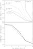 |
Fig. 7 Density diagnostic plot using the [O iii]88/opt ratio (top) and the [O iii]88/52 ratio (bottom). The [O iii]88/opt ratio depends mostly on the electron temperature for T ≲ 8000 K. Results were computed with Cloudy using a half-solar metallicity (Sect. 6.2). |
5.4. Low-excitation ionized gas tracers
The [N ii]122 and [N ii]205 lines trace the low-excitation ionized gas (the N+ ion exists for energies >14.5 eV). The critical density of [N ii]122 (ncr ≈ 400 cm-3) is similar to that of [O iii]88 (Table 1). [N ii]122 was only barely detected toward a few positions in the mapping observation because of a too short integration time. The upper limit on the total emission in the map is <5.5 × 10⁻¹⁵ W m-2. The follow-up pointed observations successfully detected [N ii]122 toward W2 and W1, with peak emissions of 1.4 × 10⁻⁸ W m-2 sr-1 and 8.5 × 10⁻⁹ W m-2 sr-1, respectively.
Unfortunately, [N ii]205 was not detected in the mapping observation. The upper limit on the total emission in the map is <3.6 × 10⁻¹⁵ W m-2. Since the [N ii]122 is systematically brighter than [N ii]205 for densities over 10 cm-3 (Oberst et al. 2006), the upper limit on [N ii]205 is not a useful constraint on the gas density and on the models discussed in this paper.
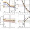 |
Fig. 8 Line flux ratios plotted against the ionization parameter U for radiation temperature of Teff = 40 000 K (orange models) and 45 000 K (blue models). The horizontal lines show the observed values toward specific regions illustrated in previous figures, while the associated vertical bars show the range of values within each region. The light gray horizontal rectangle shows the range of values observed across the entire N 11B nebula. The dark gray vertical rectangle indicates the range of U values agreeing the best with the observed line ratios (see text). The vertical arrow shows the effect of dust extinction on the observations for AV = 1. The W1 region was not covered by the [O iii]opt HST/WFPC2 observation (Fig. 6), and [N ii]122 was only detected by the Herschel/PACS follow-up pointed observations (Fig. 4). |
6. Physical conditions of the ionized gas
6.1. Contribution from shocks
The presence of shocks from supernovae remnants or from stellar winds could modify the electronic level population and therefore line ratios. A diffuse soft X-ray emission component was detected in N 11B (Mac Low et al. 1998; Nazé et al. 2004), and wind-blown bubbles around individual stars or groups of stars were detected kinematically by Nazé et al. (2001). These bubbles are all X-ray emitters despite their low expansion velocities of 10–15 km s-1. On the other hand, as noted in Nazé et al. (2001), the young age of the LH 10 association, as opposed to the central association of N 11 (LH 9), suggests that the most massive stars did not have time to evolve into supernovae. Strong interstellar shocks are therefore not expected in N 11B.
To verify these assumptions, we compared the observed line ratio [O iii]88/opt to the predictions from the shock model described in Allen et al. (2008). For LMC abundances and a density of 1 cm-3, the [O iii]88/opt ratio in the shocked gas is always lower than ≈0.23 throughout the range of velocity and magnetic field values in the model. A somewhat lower ratio would be obtained for densities higher than 1 cm-3. Accounting for the extinction by dust (which affects the optical line emission at least toward W2 and LH 10; Sect. 6.3), our observations show that [O iii]88/opt ≳ 0.25 across the nebula (Fig. 8c). As a result one can see that (1) shocks will tend to lower the observed [O iii]88/opt ratio, and (2) although shocks might exist, they do not dominate the ionization structure of the N 11B nebula.
6.2. Photoionization modeling
In the following, we model the physical conditions in the N 11B nebula with the photoionization code Cloudy (c10.00; Ferland et al. 1998). A single stellar source is used to model the radiation field. We used the stellar atmosphere grid WM-Basic (Pauldrach et al. 2001, and references therein) because it includes non-LTE effects. The stellar grid was computed with half-solar metallicity and main-sequence parameters. The intensity of the radiation field varies through the ionization parameter U, which is defined as  (1)where Φ(H) is the flux of ionizing photons per unit surface and n(H) is the hydrogen density. The other varying parameters are the stellar radiation effective temperature Teff and the gas density n (assumed to be constant). The main parameters for the models are listed in Table 4. Models are stopped at the ionization front, i.e., when the electron fraction reaches 0.5. Figure 8 shows the line ratios predicted by the models, together with the observations toward specific regions in the map (the compact regions W1 and W2, the stellar cluster LH 10, and the relatively diffuse northern region; Sect. 2.1).
Main parameters for the models.
The observed [N iii]/[O iii]88 ratio is compatible with ionization parameters ≳−3 and with stellar temperatures between ~40 000 K and ~45 000 K (Fig. 8a). Such temperatures correspond to O7-O5 main sequence stars, many of which are detected in N 11B (Sect. 7). Only a couple of more massive stars than O5 were detected that must drive Teff slightly higher. Inversely, radiation temperatures colder than 40 000 K fail to reproduce the observed [N iii]/[O iii]88 ratio because corresponding models produce too little [O iii]88 emission.
Considering that the gaseous nebula in N 11B should have a density higher than >10 cm-3 (Sect. 2.3), the average [N iii]/[O iii]88 ratio in each region (Fig. 8a) is compatible with an ionization parameter ~− 2 for a radiation temperature of Teff = 40 000 K and ~− 3 for Teff = 45 000 K. Still, [N iii]/[O iii]88 shows significant variations across N 11B, by a factor of ~5. The lowest value is found in LH 10 and agrees with both low-density and high ionization-parameter. Inversely, the highest value is found in the northern region and it agrees with a low ionization-parameter (~− 3), which is expected from the larger distance to the known ionizing clusters.
For illustration, an ionization parameter of −2 would correspond to a 25 cm-3 cloud located 6 pc from a O5 V star (U = −1 implies a distance of 2 pc while U = −3 implies 18 pc) or to a 200 cm-3 cloud located 2 pc away. A lower limit of 5 pc can be set on the distance between the W2 ionization fronts and most stars in LH 10 by measuring the projected distance in Fig. 2. Considering the large number of ionizing stars in LH 10 (Sect. 2.2), it is surprising to find such a low ionization parameter. However, we note that the flux of all the ionized gas tracers (Hα, [O iii]88,opt, [N iii], and [N ii]122) is in fact only twice greater toward W2 than toward the surrounding regions, so half of the ionization must come from an extended gas component, which has likely a lower U value because of geometrical dilution. We thus expect a very low-density component that drives U lower (see also Sect. 7). Choosing a density of ne = 25 cm-3 and a distance of 30 pc (size of the PACS map coverage), log U = −2 corresponds to about 26 O5 V sources, which is a realistic number considering the O star census in N 11B (Sect. 7).
[N ii]122/[N iii] is another useful tracer of the physical conditions in the ionized gas, as it usually provides an estimate of Teff (e.g., Rubin et al. 1994). This ratio is also geometry-dependent because [N ii]122 emits close to the ionization front, so that the nebula should be radiation-bounded for the derived physical conditions to be meaningful. We now test this hypothesis. [N ii]122 was only detected toward the brightest regions W1 and W2 (Fig. 4). Figure 8b shows that [N ii]122/[N iii] toward W1 and W2 is compatible with an ionization parameter in the range [−2.5,−1.8] (ne ~ 100 cm-3 and Teff = 40 000 K). We obtain the same range from the [N iii]/[O iii]88 diagnostic plot, implying that [N ii]122/[N iii] provides a good estimate of the physical conditions toward W1 and W2; i.e., the nebula must be radiation-bounded toward these two positions. This agrees with the optical images that show multiple ionization fronts (Sect. 2.1). If the nebula was not radiation-bounded, we should have observed a lower [N ii]122/[N iii] ratio, which in turn would have translated into a larger U parameter. Unfortunately, we cannot conclude anything about the other regions, since [N ii]122 was detected only toward W1 and W2.
The diagnostic plots in Fig. 8 give useful indications about the excitation conditions within the compact source W1. The ratios [N ii]122/[N iii] and [N iii]/[O iii]88 toward W1 are similar to the values within W2. Assuming that the same radiation field temperature holds for both regions (~45 000 K), this implies roughly the same ionization parameter. Given the small size of W1 (1 pc; Fig. 2), we could have expected a much larger U. That U is the same toward W1 and W2 is a strong indication that sources within W1 do not dominate the ionization of the region. Instead, it is likely that the ionization fronts are due to sources outside W1. These sources are very likely the massive stars in the “footprint” cluster and in LH 10. This was hypothesized by Nazé et al. (2001) based on the orientation of the ionization fronts as seen from the optical images. Sources within W1 must be much colder than 40 000 K, resulting in a larger U parameter but a much weaker and, in fact, negligible [O iii]88 flux.
6.3. Evidence of obscured ionized gas
We now investigate the dust extinction by comparing [O iii]88 and [O iii]opt. The FIR line is not affected by dust extinction and potentially provides a better handle on the spatial distribution of the ionized gas. Furthermore, understanding the extinction across N 11B allows us to use the [O iii]opt/Hα ratio as a diagnostic tool for the physical conditions.
The relative variations of [O iii]opt and [O iii]88, which intrinsically depend on the electron density and temperature (Sect. 5), is then modified by dust extinction, which significantly affects the emission from the optical line emission. The variation in [O iii]88 and [O iii]opt between LH 10 and W2 is remarkably different, the FIR line emission being only 2.5 times lower toward W2 than toward LH 10, while the optical line is ten times weaker toward W2 than toward LH 10 (Figs. 4 and 6). This could be due a priori to a variety of parameters (different line critical densities, different electron temperature, extinction by dust).
Figure 8c shows that [O iii]88/opt is systematically underestimated by all models. The most relevant models for comparison to observations have densities around (~10–100 cm-3; long- and short-dashed lines) and U ~ −2 (Sect. 6.2). As shown in Fig. 7, [O iii]88/opt varies with the electron density and temperature. Tsamis et al. (2003) find a large discrepancy between optical recombination vs. collisionally-excited lines of O+, but they note that this difference cannot be explained either by temperature fluctuations in a chemically and density homogenous nebula or by high-density clumps.
Another caveat concerns the metal abundance. Although the observed [O iii]88/opt ratio could be reconciled with models by using a higher metallicity (since heavy elements provide more cooling, which in turn reduces the optical line emission), we consider this hypothesis as being unrealistic given the well constrained abundances in N 11B (Tsamis et al. 2003). For illustration, a solar abundance would be required for the models to reach the observed [O iii]88/opt toward W1 and LH 10.
Given the different wavelength ranges of [O iii]88 and [O iii]opt, extinction by dust plays the most important role. The effect of dust extinction with AV = 1 is shown in Fig. 8c. The average color excess towards stars across the N 11B nebula is E(B − V) ≈ 0.2, while some stars have a significantly greater reddening (Parker et al. 1992; Lee 1990). This can be compared to E(B − V) ≈ 0.05 toward the central cluster LH 9 of N 11, which is essentially foreground galactic extinction (Parker et al. 1992). Tsamis et al. (2003) find that the Balmer ratios in the optical spectra (long slit of 5.6′ × 1.5″) agree fairly well with the theoretical values in the case B with a Galactic foreground extinction. From the same Balmer ratios, we estimate that the extinction cannot be much more than E(B − V) ≲ 0.15 in the area probed by the long slit. From this value of E(B − V) = 0.15, we estimate that as much as ≈38% of the [O iii]opt emission is extinguished by dust by using the extinction curve from Cardelli et al. (1989) with a total-to-selective extinction RV = 3.1 (Howarth 1983). This leads to a lower [O iii]88/opt by a factor ≈1.6, which is high enough to reconcile most of the observations with the models.
Toward a more detailed analysis, we find that [O iii]88/opt ratio toward the stellar cluster LH 10 is a factor of ≈2 above any models. In particular, the observed ratios lie above the models with the low densities expected in that region (Sect. 2.3). Assuming that the difference between the models and the observations is driven by interstellar dust extinction, such a factor translates into a visual extinction of AV ≈ 1 or E(B − V) ≈ 0.21. This determination is in good agreement with the average color excess E(B − V) = 0.2 toward the stars.
The situation toward W2 is more complex. If the line emission is dominated by low-density ionized gas, then almost no dust extinction is required since the observed [O iii]88/opt is close to the 10 cm-3 track. On the other hand, if the emission is dominated by denser gas (Sect. 2.1), then a factor 1.5–2 could be required, translating into E(B − V) ~ 0.12–0.2. Finally, the [O iii]88/opt ratio toward the northern region is also close to the lowest density tracks, requiring only little dust extinction (AV ~ 0.5).
We thus get the picture of a low-density nebula emission that is hardly attenuated by dust extinction, except toward the stellar cluster LH 10 and possibly W2. Is the required extinction compatible with the amount of dust available? We now determine the maximum dust extinction across the region. The maximum extinction is given by the total amount of dust available. We built the extinction map from the modeling of the spatial distribution of the dust mass derived by Hony et al. (in preparation). The grain emission is constrained by the Spitzer and Herschel data of N 11. The grain composition is the “Amorphous carbon model” of Galliano et al. (2011), since it is the model that gives gas-to-dust mass ratios that are consistent with the elemental abundances in the LMC. In addition, it provides a conservative estimate, since it gives a lower dust mass, hence a lower AV. The dust mass derived from SED modeling is turned into an AV by using  (2)where Apix = 124pc2 is the surface of the pixel used for the modeling, and κext(V) = 3175m2/kg is the V band opacity of the grain mixture (Fig. A.1 of Galliano et al. 2011). Equation (2) corresponds to the maximum extinction since it corresponds to the AV of the entire LMC toward the line of sight. The
  calculated from the dust modeling ranges from ~1 to ~16 in the area observed by the PACS FIR lines, with a median value of 3. is ~1.4 toward LH 10, ~5–16 toward W2, and ~3–4 toward the northern region. We call here that the actual extinction AV corresponds to the dust fraction between and the relevant emission source (here the emission-lines from the ionized gas). Without a precise knowledge of the morphology of the region, this fraction lies anywhere from 0 to 1. We nevertheless conclude that there is enough dust to explain an extinction of AV ~ 1 toward LH 10 and W2.
Correcting for dust extinction with AV ~ 1 toward LH 10 and W2, we find that [O iii]opt/Hα toward these two regions is in reality significantly greater than toward the northern region (Fig. 8d). This is simply explained by the larger distance between the stellar cluster and the northern region, which reduces the ionization parameter.
7. Spatial extent of the [O III] emission
We observe that the [O iii]88 emission is spread throughout the N 11 nebula. Is the [O iii]88 emission compatible with the number of known massive stars and their spatial distribution? The ISM density structure plays a dominant role in controlling the mean free path of FUV photons. The presence of [O iii]88 emission significantly far away from any massive star is a strong indication that photons are able to travel through a low-density material and/or that the ISM is significantly porous. We now attempt to model the [O iii]88 emission around each massive star in order to constrain an upper limit on the density above which FUV photons are not able to travel to large distances.
We consider the O stars identified by Parker et al. (1992) (Table 5) since cooler stars are not able to ionize significant amounts of oxygen into O++ (Sect. 2.2). It must be noted that unidentified embedded massive stars can contribute to the [O iii]88 emission. Furthermore, for several stars, the identification could be uncertain because of multiple stars combined in the same spectrum. While the spectral type derived from the composite spectrum can be correct, the number of sources (and thus the number of ionizing photons) might be different. The number of O stars given in Table 5 should be considered as a lower limit.
O stars with known spectral types.
We assume in the following that stars excite their own surrounding nebula (i.e., photoionization is radiation-bounded) and that the density is homogenous. The stellar properties (number of ionizing photons, temperature) are taken from Sternberg et al. (2003). Figure 9 shows the [O iii]88 emitting spheres around each O star in N 11B. The emissivity from the Cloudy models around each star was computed assuming a uniform spherical geometry and projected on the sky at the distance of N 11B. The final maps (Fig. 9) were created by coadding the individual models.
It can be seen that models with a density of ≳100 cm-3 predict a small ionized volume as compared to the physical scale of N 11B. As the density decreases, FUV photons are able to travel farther away and ionize the ISM several tens of parsecs from the star. A density around 8–16 cm-3 seems to reproduce the physical extent of N 11B well. The [O iii]88 extent for each O star is given in Table 5 for a density of 16 cm-3. The largest diameter at a density of 16 cm-3 reaches ≈40 pc, for PGMW 3061, 3058, 3053, and 3209, which is close to the physical size of N 11B (≈80 × 60 pc from the Hα image). We conclude that it is possible for the O stars to excite [O iii]88 throughout the PACS map, provided some low-density channels exist that are as low as ≲16 cm-3. This value is significantly less than the densities from the optical doublet diagnostics (~100 cm-3, Sect. 2.3), and it suggests that the optical line measurements are biased toward the brightest and possibly densest regions.
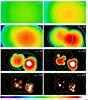 |
Fig. 9 [O iii]88 distribution modeled around each star with an homogeneous density ranging from 2 cm-3 to 256 cm-3. The yellow polygon indicates the PACS coverage and the green polygon indicates the approximate extent of the optical body. The cyan circles in the n = 16 and 32 cm-3 panels represent the extent of the [O iii]-emitting zone when considering a cluster instead of the individual stars (see text). |
Although the absorption of UV photons is mostly due to the gas rather than to the dust, dust does play an important role in determining the mean free path of UV photons. It is therefore interesting to consider a cluster of stars ionizing the ISM around it rather than a collection of separate individual stars. Models with stars gathered in clusters remove the assumption that each star excites their own surrounding nebula. We therefore now consider two main regions powered by their own stellar cluster. The western half of N 11B is dominated by the LH 10 southern cluster and the eastern half by the “footprint” cluster (Fig. 9). The nebular density best agreeing with the physical size of N 11B is around ≲16 cm-3. The radius corresponding to each cluster is reported in Table 5 and shown in Fig. 9. The volume ionized by the clusters is slightly smaller than the sum of the individual volumes around each star for a given region (by 17% and 9% lower for the western and eastern halves, respectively). Although the exact location of the cluster centroid is quite uncertain since stars are in reality not co-spatial, the overall [O iii] extent of the two clusters encompasses the N 11B nebula relatively well.
We conclude that massive stars in N 11B are able to produce [O iii]88 emission at large distances in the global low-density medium of N 11B. Although higher density material does exist, the low-density regions provide channels for the FUV photons to permeate into the ISM. For instance, the northern region shows significant [O iii]88 emission, while there are no ionizing sources, implying that FUV photons were able to cross most of the N 11B nebula. The global density of ≲16 cm-3 that we derive is an upper limit, since projection effects prevent us from asserting the depth of the nebula in detail so that distances are in fact lower limits to the actual distances. Slightly larger distances would then require slightly lower densities in order to reach further. Another caveat should be added that we assumed a gas filling-factor of 1. If the gas were to fill only a fraction of the nebula, UV photons would travel even farther for a given density.
8. Origin of the [C II] emission
Because of its low excitation temperature, [C ii] can potentially emit from several ISM phases (see introduction). The [C ii] emission peaks toward W2, but it is dominated by extended emission (Sect. 5.2). The [C ii] distribution is characterized by a sharp decrease in flux toward the stellar cluster LH 10, contrasting with the flat [O iii]88 emission (Fig. 4). In Fig. 10, it can be seen that the spatial distributions of [O iii]88 and [C ii] are anti-correlated to first order, except toward W2 where all the FIR tracers are concentrated. The [O iii]88 emission thus appears to surround lower ionization regions, which might be associated to PDRs. In the following we now investigate the possible contribution from the ionized gas and from PDRs to the [C ii] emission. We use [N ii]122 and [O iii]88 to trace the low-density ionized gas, and [O i]63 and PAH emission to trace PDRs.
8.1. Ionized gas component
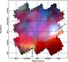 |
Fig. 10 Three-color image of the following PACS lines, [C ii] (blue), [O i]63 (green), and [O iii]88 (red). |
Most of the ionized gas in N 11B has a density around or lower than the critical density of [C ii] (80 cm-3 for collisions with e−; Table 1), so we expect most of the C+ in the ionized phase to de-excite radiatively in the ionized gas. Figure 11 shows that the [C ii] emission is systematically underestimated by the models. We wish to call here that our models correspond to the photoionized gas in the H ii region and that calculations were stopped at the ionization front (see Sect. 6.2). An important warning is that [C ii] in the ionized gas is expected to emit close to the ionization front, so that our results strongly depend on the geometry and on the radiation-bounded nature of the nebula. While the compact regions W1 and W2 appear to be radiation-bounded (Sect. 6.2), the situation is uncertain for the more diffuse and extended regions. Therefore, the model predictions for [C ii] emission should be considered as upper limits except toward W1 and W2. With these caveats in mind, we assume a density between 10 cm-3 and 100 cm-3, and from Fig. 11 we estimate that the fraction of [C ii] originating in the ionized gas is ~15% toward LH 10 and ~4% toward the northern region, while it is ≲4% toward W1 and ≲2% toward W2.
The [N ii]122 line is a good tracer of the diffuse ionized gas from which [C ii] could also arise (e.g.; Oberst et al. 2006). [N ii]122 and [C ii] involve similar energies (ions existing for energies >14.5 eV and >11.3 eV respectively), but they have significantly different critical densities in the ionized gas (≈400 cm-3 and ≈80 cm-3, respectively, for collisions with e−). Even for densities as low as ~50 cm-3, therefore, the de-excitation of [C ii] in the ionized gas is affected by collisions, and the [N ii]122/[C ii] ratio thus increases with density until the critical density of [N ii]122 is reached. [N ii]122 was detected only toward the compact regions W1 and W2 with pointed observations (Sect. 5). The PACS footprint size unfortunately barely samples the extended emission around these two regions (Fig. 4). Figure 11 shows that [N ii]122/[C ii] toward W1 and W2 is significantly lower than the models with ne ~ 100 cm-3, confirming that most of [C ii] arises in PDRs toward these regions. The ISO observation (Sect. 4.2) shows that [N ii]122/[C ii] ≲ 0.03 in the 80′′ beam, which includes W2. It thus seems that our results remains unchanged on a larger scale; i.e., [N ii]122/[C ii] is lower than expected from the ionized gas, and most of [C ii] toward W1 and W2 originates in PDRs.
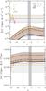 |
Fig. 11 The integrated emission of [C ii] (top) and the [N ii]122/[C ii] ratio (bottom) are plotted against the ionization parameter U. Models show the expected values in the ionized gas of the H ii region. See Fig. 8 for the plot description. |
8.2. PDR component
Our results suggest that most of the [C ii] emission in N 11B does not originate in the ionized gas (Sect. 8.1). However, the uncertainty on the ionization structure and the low S/N of the ionized gas tracer [N ii]122 observation prevents a conclusive result for the most diffuse regions (i.e., other than the regions W1 and W2). We now investigate the relation between gas heating tracers (e.g., TIR and PAH emission) and gas cooling tracers (e.g., [C ii] and [O i]63) to understand the origin of [C ii] and also to constrain the dominant gas heating source in PDRs.
8.2.1. Gas heating
The gas heating in PDRs and in neutral atomic clouds is dominated by the photoelectric effect on dust grains (e.g., Hollenbach & Tielens 1999; Weingartner & Draine 2001), in which a photoelectron is ejected from the grain following the absorption of a FUV photon. The power absorbed by dust that goes into ISM heating, referred to as the photoelectric efficiency ϵPE, is ~1%, and is the largest for small grains and neutrally charged grains (e.g., Tielens & Hollenbach 1985a). The gas heating is expected to originate about equally in PAHs (and PAH clusters) and in very small grains with radii ≲100 Å (Bakes & Tielens 1994).
Although TIR emission mostly traces classical large grains in thermal equilibrium with the interstellar radiation field, the TIR emission is a good proxy for the gas heating rate in PDRs assuming a given photoelectric efficiency. The [C ii]/TIR ratio has often been used to approximate ϵPE, under the assumptions that TIR traces the gas heating rate and that [C ii] dominates the gas cooling (e.g., Rubin et al. 2009; Israel et al. 2012, in the LMC). The TIR map we used to estimate the dust extinction in Sect. 6.3 is too coarse to compare to the FIR line maps (spatial resolution of 23″ as compared to ≈11.5″; Fig. 4). We therefore examined the correlation between TIR and single dust continuum bands in order to derive a higher resolution proxy for TIR. The following bands were considered: MIPS 24 μm, PACS 100 μm and 160 μm, and SPIRE 250 μm, with resolutions of 6″, 7″, 12″, and 17″ respectively. The continuum images were convolved to 23″ resolution and resampled to match the TIR image. The correlation between TIR and each continuum band is shown in Fig. 12. We find that TIR correlates best with the 100 μm continuum on the scale of the entire N 11 nebula and most importantly within the star-forming regions N 11A and N 11B (Fig. 12). The scatter is also the smallest for TIR/100 μm. The linear regression fit shows that the flux density ratio is TIR/100 μm = 2.70 ± 0.27. In the following, we use the 100 μm dust continuum image to trace TIR to a spatial resolution compatible with the [C ii] and [O i]63 mapping observations shown in Fig. 12.
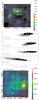 |
Fig. 12 Top − TIR map of N 11 with a resolution of 23″ (see Sect. 6.3). Middle − Correlations between TIR and individual dust continuum bands. Black points correspond to positions in N 11A and N 11B and gray points to the rest of the nebula (see top panel). The dashed line shows the average value. Bottom − TIR map using the 100 μm dust continuum as a tracer. See Fig. 4 for the figure description. |
PAH molecules and PAH clusters are expected to be important contributors to gas heating. Rubin et al. (2009) find a good correlation between [C ii] and the Spitzer/IRAC 8.0 μm band throughout the LMC and proposes that PAHs dominate the photoelectric heating rate in PDRs. In the following, we revisit these findings by using the PAH map presented in Sect. 4.2 and by examining both [C ii] and [O i]63 as potential coolants.
8.2.2. Relation between dust heating and gas cooling
Figure 13 shows the correlation between gas cooling tracers ([C ii], [O i]63, and their sum) and dust heating tracers (TIR, PAH). We use here the 100 μm dust continuum as a proxy for TIR (Sect. 8.2.1). The ratio of cooling lines to dust heating tracers provides a proxy for the fraction of the power absorbed by dust that is transferred into gas heating. The [O i]63/(TIR, PAH) ratio shows a large scatter (factor of ≈15 for [O i]63/TIR, ≈5 for [O i]63/PAH), with the lowest values toward the stellar cluster LH 10 and the northern region (Fig. 13), while the highest values are found in W1 and W2. The [C ii]/(TIR, PAH) ratio is significantly tighter than [O i]63/(TIR, PAH), with a factor of ≈6 for [C ii]/TIR and ≈4 for [C ii]/PAH. Finally, the use of the sum [C ii]+[O i]63 to trace the gas cooling provides the tightest relation with both TIR and PAH emission, with a factor of ≈4 for ([C ii]+[O i]63)/TIR and ≈2 for ([C ii]+[O i]63)/PAH. We note that the relatively large scatter of ([C ii]+[O i]63)/TIR is caused by the LH 10 region and its surroundings (see also Sect. 8.2.4). When ignoring LH 10, the scatter of ([C ii]+[O i]63)/TIR is similar to that of ([C ii]+[O i]63)/PAH.
The [C ii]/(TIR, PAH) and [O i]63/(TIR, PAH) ratios are anti-correlated in most regions. The ratios are also anti-correlated with respect to the TIR and PAH emission, with [C ii]/(TIR, PAH) decreasing with TIR and PAH emission, while the inverse is observed for [O i]63/(TIR, PAH). The anti-correlation between [C ii]/(TIR, PAH) and [O i]63/(TIR, PAH) is due to different PDR conditions, with the cooling being dominated either by [C ii] in the most diffuse regions or by [O i]63 in the densest regions and/or the regions with intense UV field (e.g., Kaufman et al. 2006). This result is compatible with the fact that [O i]63/(TIR, PAH) is relatively brighter toward W1 and W2, which are relatively dense regions located near massive stars (Sects. 2.1, 2.3). The cooling via [O i]63 represents ~25% of the total cooling rate across N 11B except toward W1 and W2 where it reaches ~50%. On large scales, we therefore expect [C ii] to be a fairly good proxy for the total cooling, which confirms the estimates made by Rubin et al. (2009). We keep in mind that the [O i]63 line could be affected by optical depth effects, more so than [O i]145 and [C ii] (e.g., Abel et al. 2007). However, only low AV values are found in N 11B (AV ≲ 1; Sect. 6.3), suggesting that optical depths effects are negligible at the spatial resolution probed by PACS (≈9.5–13′′). [C ii] and [O i]63 thus compensate for each other and, assuming these two lines are the dominant coolants at low AV (e.g., Tielens et al. 1985a; Hollenbach & Tielens 1999), the sum [C ii]+[O i]63 provides a proxy for the total gas cooling.
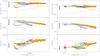 |
Fig. 13 Pixel-to-pixel correlation between the PACS cooling lines ([C ii], [O i]63, and their sum) and 2 quantities used to trace the gas heating, i.e., the TIR emission (left panel) and the PAH emission (right panel). The solid curve represents the linear regression for a given plot and the dashed curves the linear regression of the other ratios for comparison. The colors correspond to specific regions illustrated in Fig. 12. The symbol size is proportional to [C ii]+[O i]63 (top), [C ii] (middle), and [O i]63 (bottom). The gray rectangles on the left side show the values observed by Croxall et al. (2012) in 2 super-solar metallicity nearby galaxies (see text). |
8.2.3. PDR conditions
The flat correlation between [C ii]+[O i]63 and PAH (or, although to a lesser extent, TIR), together with the fact that W1 and W2 are dominated by PDRs (Sect. 8.1), suggests that [C ii] and [O i]63 originate in PDRs throughout N 11B. The scatter of ([C ii]+[O i]63)/PAH is a factor of ≈2, implying that the fraction of [C ii] originating in PDRs is at least ~50% throughout N 11B. The spatial anticorrelation between [C ii] and the warm photoionized gas probed by [O iii]88 (Fig. 10) suggests that PDRs are mainly located within the ionized gas nebula (i.e., they are not located at the edge of the N 11B region).
The small scatter of ([C ii]+[O i]63)/PAH further implies that the photoelectric efficiency in PDRs is uniform within a factor of ≈2. This implies that the grain charging parameter, related to the UV field intensity and to the electron density (e.g., Tielens & Hollenbach 1985a), is also uniform across the region. Rubin et al. (2009) find a bias toward lower [C ii]/TIR ratios in star-forming regions of the LMC, which they ascribes to relatively low photoelectric efficiency. The [C ii]/TIR in the entire N 11 nebula found by the authors, ≈0.56%, agrees with the highest values we measure in N 11B. It is therefore likely that the large beam used by Rubin et al. (2009), 14.9′, was filled by the most diffuse regions where the cooling is dominated by [C ii]. Our results also imply that [C ii]/TIR alone (or [C ii]/PAH) does not trace the photoelectric efficiency well on small enough scales.
We do not find any significant evidence of a lower photoelectric efficiency in the regions with the greatest expected UV field intensity, such as W2 or LH 10, as compared to more quiescent regions, such as the northern region. We note, however, that the ionization parameter in most regions, including W2, indicates a dilution of the UV field on large physical scales (Sect. 6.2). It is therefore possible that variations in the UV field intensity across N 11B are not large enough to modify significantly the grain charging parameter. From Fig. 13, the average ratios are ([C ii]+[O i]63)/PAH = 7% and ([C ii]+[O i]63)/TIR = 0.55%, which can be considered as proxies for the photoelectric efficiency, if either PAHs or dust probed by TIR dominate the gas heating. We investigate the dominant heating source in Sects. 8.2.4 and 8.2.5.
8.2.4. LH 10
The case of the stellar cluster LH 10 is critical to understanding the dust component responsible for the gas heating in PDRs. LH 10 is dominated by warm photoionized gas, and the gas heating is due to photoionization in addition to the photoelectric effect. Most important, relatively warmer dust contributes to the TIR emission that is not associated with the heating of the gas in PDRs probed by [C ii] and [O i]63. In Sect. 8.2.2, we found that LH 10 drives the scatter on the ([C ii]+[O i]63)/TIR ratio up. In contrast, the ([C ii]+[O i]63)/PAH ratio shows a small scatter throughout N 11B (factor of ≈2). This shows that the PAH emission describes the gas heating well even toward the stellar cluster where other dust components exist (in particular stochastically heated small grains and warm grains in thermal equilibrium with the interstellar radiation field).
The dust model presented in Sect. 6.3 indicates that the PAH abundance varies by a factor of ~10 across N 11B, with a minimal value toward LH 10 where most PAHs are likely destroyed by the radiation field. Still, ([C ii]+[O i]63)/PAH remains constant within a factor of ≈2 as compared to other regions in N 11B. PDRs therefore exist toward LH 10 and PAH emission is a good proxy for the gas-heating rate in these PDRs even toward such an extreme environment. The PAH/TIR ratio is the lowest toward LH 10, and only a fraction of TIR must originate in PDRs, about ~40%. We investigate the dominant heating source in Sect. 8.2.5.
8.2.5. Dominant gas heating source
The gas heating should be dominated by very small grains and PAHs (Sect. 8.2.1). The 24 μm dust continuum, which is often used to trace warm dust grains and stochastically heated small grains, correlates poorly with [C ii]+[O i]63, with a scatter ~5 times larger than the correlation with PAH emission (not shown in Fig. 13). On the other hand, we find a remarkable correlation between [C ii]+[O i]63 and PAH emission, suggesting that PAHs could dominate the gas heating over the dust components probed by TIR emission (Sect. 8.2.2). However, a similarly small scatter exists with TIR emission if we ignore the LH 10 region (Sect. 8.2.4). Croxall et al. (2012) also find a smaller scatter with ([C ii]+[O i]63)/PAH than with ([C ii]+[O i]63)/TIR and concludes that the integrated dust emission does not describe well the photoelectric heating where [C ii] and [O i]63 originate. Instead, photoelectrons ejected from PAHs would dominate the gas heating (see also Helou et al. 2001; Rubin et al. 2009). We consider in the following PAHs and dust grains probed by TIR emission as potential gas-heating sources.
The total gas-cooling rate Λg, traced by [C ii]+[O i]63, is equal to the gas heating rate resulting from the photoelectric effect on dust grains probed by TIR emission ( ) and on PAHs (
 ):
):  (3)where
  and
and  are the dust heating rates for dust grains and PAHs, and ϵPE,TIR and ϵPE,PAH are the corresponding photoelectric efficiencies. Assuming that both dust components contribute to the gas heating, we conclude that upper limits on ϵPE,TIR and ϵPE,PAH are given by the ([C ii]+[O i]63)/(TIR, PAH) ratio, i.e., ≈0.55% and ≈7% respectively.
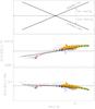 |
Fig. 14 Top − Expected trend between ([C ii]+[O i]63)/(TIR, PAH) against PAH/TIR, assuming that either PAHs or the dust grains traced by TIR dominate the gas heating. Middle and bottom − Pixel-to-pixel correlation between ([C ii]+[O i]63)/(TIR, PAH) and PAH/TIR. The solid line represents the linear regression and the dotted line represents the median value. See Fig. 13 for the plot description. |
The PAH/TIR ratio varies by a factor of ≈5 across N 11B (Fig. 14), enabling us to study the influence of PAH and TIR emission as gas-heating tracers. Figure 14 shows that ([C ii]+[O i]63)/PAH and ([C ii]+[O i]63)/TIR are a smooth function of the PAH/TIR ratio. The standard deviation around the ([C ii]+[O i]63)/PAH linear regression is remarkably small, with only 6%, while it is 15% for ([C ii]+[O i]63)/TIR. The top panel in Fig. 14 shows the trend of the ([C ii]+[O i]63)/TIR and ([C ii]+[O i]63)/PAH ratios versus PAH/TIR. When PAHs dominate the gas heating, the ([C ii]+[O i]63)/TIR ratio increases with PAH/TIR, while the inverse is true for ([C ii]+[O i]63)/PAH. We normalized each ratio to its average value and calculated that the linear regression slope is ≈−3.6 for ([C ii]+[O i]63)/PAH, while it is ≈10.3 for ([C ii]+[O i]63)/TIR. From this, we conclude that PAHs dominate the gas heating over the dust component probed by TIR emission. This implies that ϵPE,PAH is close to ≈7%, and therefore a factor of ≳12 more than ϵPE,TIR. It is possible that ϵPE,TIR is larger if we would only account for the gas heating from the smallest grains (Sect. 8.2.1).
Our results suggest that classical dust grains, which are dominating the TIR emission, do not dominate the gas heating. The fraction of the TIR emission corresponding to smaller grains certainly scales better with [C ii]+[O i]63 than the total TIR. Unfortunately, in the lack of constraints on the abundance of small grains, we cannot conclude anything about the relative importance of PAHs and very small grains as gas-heating sources.
9. Conclusions
We present the Herschel/PACS spectroscopic observation of the H ii region N 11B in the LMC. The spatial distribution of the FIR lines shows remarkable differences:
-
The emission of [O iii]88, [N iii], and [C ii] is quite flat across the map, suggesting it is dominated by extended emission. This contrasts with the [O i]63 emission, which is concentrated in a few compact regions. [O i]63 also shows an extended component, about ten times fainter than the peak emission.
-
The spatial distribution of [O iii]88 appears to be anti-correlated with that of [C ii].
In the present paper, we investigate the extended emission of the FIR tracers, while in a second paper, we will investigate the compact regions and the PDR properties. The main results of the present study follow.
-
The [O iii]88 line, with its low critical density, is an excellent probe of the extended ionized gas. It is the brightest line across the region, in particular a factor of four brighter than [C ii] (in some regions 20 times brighter).
-
By comparing [O iii]88 to the optical line [O iii] 5007 Å, we find an extinction of AV ~ 1 toward W2 and the stellar cluster LH 10, implying that a significant fraction of the ionized gas is hidden in the optical. The dust mass measured in N 11B is compatible with such extinctions. The extinction AV is between ~0.5 and ~1 toward the other regions.
-
The spatial extent of [O iii]88 emission could be reproduced by considering all the confirmed O stars, provided the density of the ionized gas is generally lower than ≲16 cm-3.
-
We used the [N iii]/[O iii]88 and [N ii]122/[N iii] ratios to estimate the physical conditions in the ionized gas. The average ionization parameter is compatible with relatively low-density (≲25 cm-3) gas located on average ≲30 pc away from the ionizing sources.
-
By comparing [C ii] to the low-excitation, low-density ionized gas tracer [N ii]122, we find that [C ii] mainly arises from PDRs across N 11B.
-
We examined the relation between the gas cooling in PDRs via [C ii] and [O i]63 and the gas heating traced by TIR emission and PAH emission. We find a tight correlation between [C ii]+[O i]63 and the PAH emission. Assuming [C ii] and [O i]63 are the dominant coolants at low AV, the sum of [C ii] and [O i]63 provides a proxy for the total cooling, with [C ii] being the dominant coolant in most regions characterized by a diffuse ISM, and [O i]63 contributing significantly (up to ≈50%) in the brightest and densest regions.
-
The scatter of the ([C ii]+[O i]63)/TIR ratio is greater than that of ([C ii]+[O i]63)/PAH, which is mostly due to the stellar cluster LH 10 where another dust component, unrelated to PDRs, drives TIR to higher values.
-
We find that PAHs dominate the gas heating in PDRs, with a photoelectric efficiency of ~7%.
Online material
Appendix A: The PACSman suite for Herschel/PACS spectroscopy data analysis
PACSman4 is an IDL package designed to provide an alternative for several reduction and analysis steps performed in HIPE on PACS spectroscopic data. The following operations are currently included: transient correction, line fitting, map projection, and map analysis. All of the observation modes are supported: wavelength switching (now decommissioned), unchopped scan, and chop/nod.
A.1. Transient correction
Transients are cosmic ray hits to the detector that modify the pixel response over a given period of time (see the works of Coulais & Abergel 1999, 2000, for the ISOPHOT and ISOCAM detectors on ISO). Two types of transients are observed in the PACS data, “dippers” that result in a lower pixel response and “faders” that result in a larger pixel response. The response after a dipper hit normalizes after a short time (about the timescale of a line scan), while the response after a fader hit takes considerably longer to settle (near the observation itself or even more). A fader is often seen after the calibration block, which observes a bright source. The transient correction is only necessary for unchopped scan observations since the fast chopping in chop/nod observations allows reliable removal of the transients (dippers and faders).
A.1.1. Faders
Faders are responsible for large jumps in the flux, which can render a spectral pixel useless unless its signal is aligned with the others. HIPE includes a task called specLongTermTransient that minimizes the scatter of points by using a series of exponential functions to model the “faders” transients (Fadda & Jacobson 2011). However, it is possible that several transients overlap in time, which makes it difficult to find the number of exponential functions required and the parameters of each function. This is the main reason we developed a special routine in PACSman that performs the transient correction on the signal timeline for each of the 16 spectral pixels and each of the 25 spaxels.
PACSman includes a correction tool that uses a multiresolution algorithm to straighten the signal (Starck et al. 1999). The smallest resolution scales are subtracted to remove the noise and the largest scale is subtracted to remove any fader-type signal (Fig. A.1). The main advantage of multiresolution over an exponential curve fitting is its ability to remove the signal from several faders that are overlapping in time. Furthermore, it provides an unbiased approach since the faders do not need to be identified beforehand.
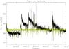 |
Fig. A.1 Example of fader transients occurring in unchopped scan observations. The signal is plotted against the readout number for a given spaxel and spectral pixel. The irregular black curve is the unflagged data, while the flat green curve shows the corrected signal. Several transients are observed in this timeline, including the systematic transient after the calibration block on the extreme left. |
A.1.2. Dippers
The presence of dippers dominates the S/N in the timeline (thus in the spectra as well). Dippers are searched for after each flagged pixel. An exponential curve is fitted with free parameters. If the timescale parameter is consistent with a dipper signal, the fit is used to correct the signal (Fig. A.2).
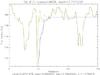 |
Fig. A.2 Example of a dipper fit. The profile is fitted by an exponential curve whose parameters are compared to the expected behavior of a dipper (in particular the timescale). |
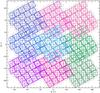 |
Fig. A.3 Example of a map projection. The observation (3 × 3 raster footprints) is shown with color symbols. The squares show the spaxel center (5 × 5 spaxels for one raster position), the large diamond shows the spaxels (1, 1), and the dots show the center of the subspaxel (1 / 3 of the size of a spaxel). The information from different spaxels and rasters can be combined to populate the projected grid. Subpixels where there is no coverage are shown as gray squares. |
A.2. Line fitting
The input data for line fitting and map projection (Sect. A.3) is the Level 1 cube reduced with HIPE. At this level of reduction, the data is calibrated in flux and in wavelength. The bad pixels are masked according to the HIPE reduction criteria (outliers, glitches, saturated, noisy, etc.). The data cube contains one spectral window for each of the 25 spaxels and 16 spectral pixels (and for a given raster position when mapping). The HIPE reduction corrects for the flat-fielding of the spectral pixels so that the combination of the spectral windows from the 16 spectral pixels provides one spectrum per spaxel. The data cloud for a given spaxel typically contains a few million points (for line spectroscopy).
The line fitting in PACSman is performed on the full data cloud; i.e., the data is not rebinned beforehand. This is to keep all the possible information on the data and on the masks during the line fitting process. The data cloud does not provide propagated errors for the individual measurements. We estimate the error by calculating the dispersion of measurements in a given wavelength bin (defined as 1/5 of the line FWHM). By default, a 5σ clipping is performed prior the line fitting.
Line fitting is then performed with the MPFIT package5. The continuum is adjusted first using spectral windows on each side of the line. The result is then used as an initial guess for the final fit that combines the continuum polynomial and the Gaussian curve. Default constraints exist that can be changed on the line FWHM, line central wavelength, and continuum range around the line. It is essential that constraints exist to provide reliable upper limits in faint lines. For a chop/nod observation, the two nods can either be combined in a single spectrum or considered individually. The fitting is performed as follows: (1) the continuum is fitted first around the line, and (2) the line+continuum profile is fitted using the continuum fit as a first guess. Example of fits are shown in Fig. 3.
A.3. Map projection
For a mapping observation, the raster footprints (5 × 5 spaxel image of the line flux) have to be combined to create the final map. Maps are projected on a subpixel grid with a pixel size three times smaller (linear scale) than the spaxel size. The pixel size is
about 3″. This allows recovering the best spatial resolution possible (see PACS ICC calibration document PICC-KL-TN-038).
The grid orientation is chosen to be orthogonal with the raster maps so that the splitting of the spaxels requires as little rotation as possible. Since the spaxel positions and sizes are not regular, the orthogonality is only approximate. For a given pixel in the projected grid, the contributing fraction of each spaxel in the map is calculated assuming a uniform surface brightness within a spaxel (Fig. A.3). Several determinations are thus obtained for each pixel in the projected grid. The final image simply averages these determinations to obtain one value per pixel.
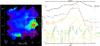 |
Fig. A.4 Example of a line cut across the map. The circles on the left image show the aperture used for extraction while the line shows the profile cut. |
A.4. Map analysis
A tool is provided to analyze the spectral maps. Several tasks can be performed, such as aperture extractions with annulus subtraction (see Figs. A.4). A 2D Gaussian surface can also be fitted to the data to estimate the source spatial FWHM. Finally, spatial profiles can also be plotted along a given cut.
As noted in Vermeij et al. (2002), the “N 11A” LWS observation is in fact pointed toward N 11B.
Available at http://www.myravian.fr or by email contact (myravian@gmail.com).
Acknowledgments
V. L. is supported by a CEA/Marie Curie Eurotalents fellowship. PACS has been developed by a consortium of institutes led by MPE (Germany) and including UVIE (Austria); KU Leuven, CSL, IMEC (Belgium); CEA, LAM (France); MPIA (Germany); INAF-IFSI/OAA/OAP/OAT, LENS, SISSA (Italy); IAC (Spain). This development has been supported by the funding agencies BMVIT (Austria), ESA-PRODEX (Belgium), CEA/CNES (France), DLR (Germany), ASI/INAF (Italy), and CICYT/MCYT (Spain). HCSS, HSpot, and HIPE are joint developments by the Herschel Science Ground Segment Consortium, consisting of ESA, the NASA Herschel Science Center, and the HIFI, PACS and SPIRE consortia. We thank Y. Nazé for providing us with the calibrated HST images. This research made use of Montage, funded by the National Aeronautics and Space Administration’s Earth Science Technology Office, Computation Technologies Project, under Cooperative Agreement Number NCC5-626 between NASA and the California Institute of Technology. Montage is maintained by the NASA/IPAC Infrared Science Archive.
References
- Abel, N. P., Sarma, A. P., Troland, T. H., & Ferland, G. J. 2007, ApJ, 662, 1024 [NASA ADS] [CrossRef] [Google Scholar]
- Allen, M. G., Groves, B. A., Dopita, M. A., Sutherland, R. S., & Kewley, L. J. 2008, ApJS, 178, 20 [Google Scholar]
- Asplund, M., Grevesse, N., Sauval, A. J., & Scott, P. 2009, ARA&A, 47, 481 [NASA ADS] [CrossRef] [Google Scholar]
- Bakes, E. L. O., & Tielens, A. G. G. M. 1994, ApJ, 427, 822 [NASA ADS] [CrossRef] [Google Scholar]
- Bakes, E. L. O., & Tielens, A. G. G. M. 1998, ApJ, 499, 258 [NASA ADS] [CrossRef] [Google Scholar]
- Barbá, R. H., Rubio, M., Roth, M. R., & García, J. 2003, AJ, 125, 1940 [NASA ADS] [CrossRef] [Google Scholar]
- Bernard-Salas, J., Habart, E., Arab, H., et al. 2012, A&A, 538, A37 [NASA ADS] [CrossRef] [EDP Sciences] [Google Scholar]
- Boreiko, R. T., & Betz, A. L. 1991, ApJ, 380, L27 [NASA ADS] [CrossRef] [Google Scholar]
- Cardelli, J. A., Clayton, G. C., & Mathis, J. S. 1989, ApJ, 345, 245 [NASA ADS] [CrossRef] [Google Scholar]
- Castelli, F., & Kurucz, R. L. 2004, IAU Symp. 210, poster A20 [Google Scholar]
- Coulais, A., & Abergel, A. 1999, The Universe as Seen by ISO, 427, 61 [Google Scholar]
- Coulais, A., & Abergel, A. 2000, A&AS, 141, 533 [NASA ADS] [CrossRef] [EDP Sciences] [Google Scholar]
- Crawford, M. K., Genzel, R., Townes, C. H., & Watson, D. M. 1985, ApJ, 291, 755 [NASA ADS] [CrossRef] [Google Scholar]
- Croxall, K. V., Smith, J. D., Wolfire, M. G., et al. 2012, ApJ, 747, 81 [NASA ADS] [CrossRef] [Google Scholar]
- Dalgarno, A., & McCray, R. A. 1972, ARA&A, 10, 375 [NASA ADS] [CrossRef] [Google Scholar]
- Davies, R. D., Elliott, K. H., & Meaburn, J. 1976, MmRAS, 81, 89 [Google Scholar]
- Fadda, D., & Jacobson, J. D. 2011, BAAS, 330.01 [Google Scholar]
- Ferland, G. J., Korista, K. T., Verner, D. A., et al. 1998, PASP, 110, 761 [Google Scholar]
- Ellingsen, S. P., Whiteoak, J. B., Norris, R. P., Caswell, J. L., & Vaile, R. A. 1994, MNRAS, 269, 1019 [NASA ADS] [CrossRef] [Google Scholar]
- Evans, C. J., Lennon, D. J., Smartt, S. J., & Trundle, C. 2006, A&A, 456, 623 [NASA ADS] [CrossRef] [EDP Sciences] [Google Scholar]
- Galliano, F., Hony, S., Bernard, J.-P., et al. 2011, A&A, 536, A88 [NASA ADS] [CrossRef] [EDP Sciences] [Google Scholar]
- Garnett, D. R. 1999, New Views of the Magellanic Clouds, 190, 266 [NASA ADS] [Google Scholar]
- Grenier, I. A., Casandjian, J.-M., & Terrier, R. 2005, Science, 307, 1292 [NASA ADS] [CrossRef] [PubMed] [Google Scholar]
- Hatano, H., Kadowaki, R., Nakajima, Y., et al. 2006, AJ, 132, 2653 [NASA ADS] [CrossRef] [Google Scholar]
- Heiles, C. 1994, ApJ, 436, 720 [NASA ADS] [CrossRef] [Google Scholar]
- Helou, G., Malhotra, S., Hollenbach, D. J., Dale, D. A., & Contursi, A. 2001, ApJ, 548, L73 [Google Scholar]
- Henize, K. G. 1956, ApJS, 2, 315 [NASA ADS] [CrossRef] [Google Scholar]
- Hollenbach, D. J., & Tielens, A. G. G. M. 1999, Rev. Mod. Phys., 71, 173 [Google Scholar]
- Howarth, I. D. 1983, MNRAS, 203, 301 [NASA ADS] [CrossRef] [Google Scholar]
- Indebetouw, R., Johnson, K. E., & Conti, P. 2004, AJ, 128, 2206 [NASA ADS] [CrossRef] [Google Scholar]
- Israel, F. P., & Maloney, P. R. 2011, A&A, 531, A19 [NASA ADS] [CrossRef] [EDP Sciences] [Google Scholar]
- Kaufman, M. J., Wolfire, M. G., & Hollenbach, D. J. 2006, ApJ, 644, 283 [NASA ADS] [CrossRef] [Google Scholar]
- Kawada, M., Takahashi, A., Yasuda, A., et al. 2011, PASJ, 63, 903 [NASA ADS] [Google Scholar]
- Kennicutt, R. C., Jr., & Hodge, P. W. 1986, ApJ, 306, 130 [NASA ADS] [CrossRef] [Google Scholar]
- Kennicutt, R. C., Calzetti, D., Aniano, G., et al. 2011, PASP, 123, 1347 [NASA ADS] [CrossRef] [Google Scholar]
- Kessler, M. F., Steinz, J. A., Anderegg, M. E., et al. 1996, A&A, 315, L27 [NASA ADS] [Google Scholar]
- Kim, S., Staveley-Smith, L., Dopita, M. A., et al. 2003, ApJS, 148, 473 [NASA ADS] [CrossRef] [Google Scholar]
- Kulkarni, S. R., & Heiles, C. 1987, Interstellar Processes, 134, 87 [NASA ADS] [CrossRef] [Google Scholar]
- Lee, M. G. 1990, Ph.D. Thesis, Washington Univ., Seattle [Google Scholar]
- Lucke, P. B., & Hodge, P. W. 1970, AJ, 75, 171 [NASA ADS] [CrossRef] [Google Scholar]
- Maciel, W. J., & Pottasch, S. R. 1982, A&A, 106, 1 [NASA ADS] [Google Scholar]
- Mac Low, M.-M., Chang, T. H., Chu, Y.-H., et al. 1998, ApJ, 493, 260 [NASA ADS] [CrossRef] [Google Scholar]
- Madden, S. C., Geis, N., Genzel, R., et al. 1993, ApJ, 407, 579 [NASA ADS] [CrossRef] [Google Scholar]
- Madden, S. C., Poglitsch, A., Geis, N., Stacey, G. J., & Townes, C. H. 1997, ApJ, 483, 200 [NASA ADS] [CrossRef] [MathSciNet] [Google Scholar]
- Madden, S. C., Galliano, F., Jones, A. P., & Sauvage, M. 2006, A&A, 446, 877 [NASA ADS] [CrossRef] [EDP Sciences] [Google Scholar]
- Mochizuki, K., Nakagawa, T., Doi, Y., et al. 1994, ApJ, 430, L37 [NASA ADS] [CrossRef] [Google Scholar]
- Nazé, Y., Chu, Y.-H., Points, S. D., et al. 2001, AJ, 122, 921 [NASA ADS] [CrossRef] [Google Scholar]
- Nazé, Y., Antokhin, I. I., Rauw, G., et al. 2004, A&A, 418, 841 [NASA ADS] [CrossRef] [EDP Sciences] [Google Scholar]
- Oberst, T. E., Parshley, S. C., Stacey, G. J., et al. 2006, ApJ, 652, L125 [NASA ADS] [CrossRef] [MathSciNet] [Google Scholar]
- Osterbrock, D. E., & Ferland, G. J. 2006, Astrophysics of gaseous nebulae and active galactic nuclei, 2ndn (Sausalito, CA: University Science Books) [Google Scholar]
- Ott, S. 2010, Astronomical Data Analysis Software and Systems XIX, 434, 139 [NASA ADS] [Google Scholar]
- Palay, E., Nahar, S. N., Pradhan, A. K., & Eissner, W. 2012, MNRAS, 423, L35 [NASA ADS] [CrossRef] [Google Scholar]
- Parker, J. W., Garmany, C. D., Massey, P., & Walborn, N. R. 1992, AJ, 103, 1205 [Google Scholar]
- Pauldrach, A. W. A., Hoffmann, T. L., & Lennon, M. 2001, A&A, 375, 161 [NASA ADS] [CrossRef] [EDP Sciences] [Google Scholar]
- Pilbratt, G. L., Riedinger, J. R., Passvogel, T., et al. 2010, A&A, 518, L1 [CrossRef] [EDP Sciences] [Google Scholar]
- Pineda, J. L., Mizuno, N., Stutzki, J., et al. 2008, A&A, 482, 197 [NASA ADS] [CrossRef] [EDP Sciences] [Google Scholar]
- Poglitsch, A., Waelkens, C., Geis, N., et al. 2010, A&A, 518, L2 [NASA ADS] [CrossRef] [EDP Sciences] [Google Scholar]
- Röllig, M., Ossenkopf, V., Jeyakumar, S., Stutzki, J., & Sternberg, A. 2006, A&A, 451, 917 [NASA ADS] [CrossRef] [EDP Sciences] [Google Scholar]
- Rosado, M., Laval, A., Le Coarer, E., et al. 1996, A&A, 308, 588 [NASA ADS] [Google Scholar]
- Rubin, D., Hony, S., Madden, S. C., et al. 2009, A&A, 494, 647 [NASA ADS] [CrossRef] [EDP Sciences] [Google Scholar]
- Stacey, G. J. 1985, Ph.D. Thesis [Google Scholar]
- Starck, J. L., Abergel, A., Aussel, H., et al. 1999, A&AS, 134, 135 [NASA ADS] [CrossRef] [EDP Sciences] [Google Scholar]
- Stasińska, G. 2002, Rev. Mex. Astron. Astrofis. Conf. Ser., 12, 62 [Google Scholar]
- Sternberg, A., Hoffmann, T. L., & Pauldrach, A. W. A. 2003, ApJ, 599, 1333 [NASA ADS] [CrossRef] [Google Scholar]
- Tielens, A. G. G. M., & Hollenbach, D. 1985a, ApJ, 291, 722 [NASA ADS] [CrossRef] [Google Scholar]
- Tielens, A. G. G. M., & Hollenbach, D. 1985b, ApJ, 291, 747 [NASA ADS] [CrossRef] [Google Scholar]
- Tsamis, Y. G., Barlow, M. J., Liu, X.-W., Danziger, I. J., & Storey, P. J. 2003, MNRAS, 338, 687 [NASA ADS] [CrossRef] [Google Scholar]
- Vermeij, R., Damour, F., van der Hulst, J. M., & Baluteau, J.-. P. 2002, A&A, 390, 649 [NASA ADS] [CrossRef] [EDP Sciences] [Google Scholar]
- Walborn, N. R., & Parker, J. W. 1992, ApJ, 399, L87 [NASA ADS] [CrossRef] [Google Scholar]
- Walborn, N. R., Drissen, L., Parker, J. W., et al. 1999, AJ, 118, 1684 [NASA ADS] [CrossRef] [Google Scholar]
- Watson, W. D. 1972, ApJ, 176, 103 [NASA ADS] [CrossRef] [Google Scholar]
- Weingartner, J. C., & Draine, B. T. 2001, ApJS, 134, 263 [NASA ADS] [CrossRef] [MathSciNet] [Google Scholar]
- Wolfire, M. G., Hollenbach, D., McKee, C. F., Tielens, A. G. G. M., & Bakes, E. L. O. 1995, ApJ, 443, 152 [Google Scholar]
- Wolfire, M. G., Hollenbach, D., & McKee, C. F. 2010, ApJ, 716, 1191 [NASA ADS] [CrossRef] [Google Scholar]
- Wu, Y., Charmandaris, V., Hao, L., et al. 2006, ApJ, 639, 157 [NASA ADS] [CrossRef] [Google Scholar]
All Tables
All Figures
|
Fig. 1 The giant H ii region N 11, with Spitzer/MIPS 24 μm shown in red, Spitzer/IRAC 8.0 μm in green, and H i column density (from Kim et al. 2003) in blue. The Spitzer/MIPS 24 μm emission is dominated by very small grains that are stochastically heated and by big, warm, dust grains in thermal equilibrium with the interstellar radiation field. Spitzer/IRAC 8.0 μm emission is dominated by PAHs. The polygon shows the Herschel/PACS spectroscopic observations of N 11B presented in this paper. |
| In the text | |
|
Fig. 2 Top − HST/ACS color-composite image of the N 11B region (blue: F814; green: F658N/Hα; red: F660N/[N ii]). Images were downloaded from the Hubble Legacy Archive (http://hla.stsci.edu/) and later stitched with Montage (http://montage.ipac.caltech.edu/). The white stripes correspond to a gap between individual exposures. The yellow polygon indicates the field-of-view of the Herschel/PACS observations ( ≈ 2.3′ × 2.3′). The 4 rectangles in color indicate specific regions discussed in the text. The dashed circles represent the ISO-LWS observation (from 65′′ to 80′′FWHM beam) and the slit represents the optical observation by Tsamis et al. (2001). Bottom − Close-up of the eastern (left panel) and western (right panel) sides. The stellar complexes are labeled as the brightest star with a “+” sign appended. |
| In the text | |
|
Fig. 3 Line fits are shown for one spaxel observing the W2 region. The histogram shows the rebinned data, the thin curve shows the continuum, and the thick curve shows the fit. The fit was performed on the data cloud, which contains ≈ 140 000 points. We show the rebinned spectrum for display purposes. |
| In the text | |
|
Fig. 4 Herschel/PACS maps (in J2000 coordinates). The colorbar gives the flux in W m-2 sr-1. The dashed rectangles correspond to the zones described in Fig. 2 and Sect. 2.1. The spatial resolution is about ≈ 9.5″ for [N iii]57, [O i]63, and [O iii]88, ≈ 11.5″ for [N ii]122, [O i]145, and [C ii]157. |
| In the text | |
|
Fig. 5 ISO LWS spectrum of N 11B. See Fig. 2 for the location of the observation pointing. The colors correspond to the different spectral orders. The [O iii]88 is observed in 2 spectral orders with different spectral resolutions. The displayed spectrum was extracted using a point-like source calibration. |
| In the text | |
|
Fig. 6 [O iii]opt, Hα, and PAH maps, from top to bottom. The images were convolved at the resolution of the Herschel [C ii] map. See Fig. 4 for the figure description. |
| In the text | |
|
Fig. 7 Density diagnostic plot using the [O iii]88/opt ratio (top) and the [O iii]88/52 ratio (bottom). The [O iii]88/opt ratio depends mostly on the electron temperature for T ≲ 8000 K. Results were computed with Cloudy using a half-solar metallicity (Sect. 6.2). |
| In the text | |
|
Fig. 8 Line flux ratios plotted against the ionization parameter U for radiation temperature of Teff = 40 000 K (orange models) and 45 000 K (blue models). The horizontal lines show the observed values toward specific regions illustrated in previous figures, while the associated vertical bars show the range of values within each region. The light gray horizontal rectangle shows the range of values observed across the entire N 11B nebula. The dark gray vertical rectangle indicates the range of U values agreeing the best with the observed line ratios (see text). The vertical arrow shows the effect of dust extinction on the observations for AV = 1. The W1 region was not covered by the [O iii]opt HST/WFPC2 observation (Fig. 6), and [N ii]122 was only detected by the Herschel/PACS follow-up pointed observations (Fig. 4). |
| In the text | |
|
Fig. 9 [O iii]88 distribution modeled around each star with an homogeneous density ranging from 2 cm-3 to 256 cm-3. The yellow polygon indicates the PACS coverage and the green polygon indicates the approximate extent of the optical body. The cyan circles in the n = 16 and 32 cm-3 panels represent the extent of the [O iii]-emitting zone when considering a cluster instead of the individual stars (see text). |
| In the text | |
|
Fig. 10 Three-color image of the following PACS lines, [C ii] (blue), [O i]63 (green), and [O iii]88 (red). |
| In the text | |
|
Fig. 11 The integrated emission of [C ii] (top) and the [N ii]122/[C ii] ratio (bottom) are plotted against the ionization parameter U. Models show the expected values in the ionized gas of the H ii region. See Fig. 8 for the plot description. |
| In the text | |
|
Fig. 12 Top − TIR map of N 11 with a resolution of 23″ (see Sect. 6.3). Middle − Correlations between TIR and individual dust continuum bands. Black points correspond to positions in N 11A and N 11B and gray points to the rest of the nebula (see top panel). The dashed line shows the average value. Bottom − TIR map using the 100 μm dust continuum as a tracer. See Fig. 4 for the figure description. |
| In the text | |
|
Fig. 13 Pixel-to-pixel correlation between the PACS cooling lines ([C ii], [O i]63, and their sum) and 2 quantities used to trace the gas heating, i.e., the TIR emission (left panel) and the PAH emission (right panel). The solid curve represents the linear regression for a given plot and the dashed curves the linear regression of the other ratios for comparison. The colors correspond to specific regions illustrated in Fig. 12. The symbol size is proportional to [C ii]+[O i]63 (top), [C ii] (middle), and [O i]63 (bottom). The gray rectangles on the left side show the values observed by Croxall et al. (2012) in 2 super-solar metallicity nearby galaxies (see text). |
| In the text | |
|
Fig. 14 Top − Expected trend between ([C ii]+[O i]63)/(TIR, PAH) against PAH/TIR, assuming that either PAHs or the dust grains traced by TIR dominate the gas heating. Middle and bottom − Pixel-to-pixel correlation between ([C ii]+[O i]63)/(TIR, PAH) and PAH/TIR. The solid line represents the linear regression and the dotted line represents the median value. See Fig. 13 for the plot description. |
| In the text | |
|
Fig. A.1 Example of fader transients occurring in unchopped scan observations. The signal is plotted against the readout number for a given spaxel and spectral pixel. The irregular black curve is the unflagged data, while the flat green curve shows the corrected signal. Several transients are observed in this timeline, including the systematic transient after the calibration block on the extreme left. |
| In the text | |
|
Fig. A.2 Example of a dipper fit. The profile is fitted by an exponential curve whose parameters are compared to the expected behavior of a dipper (in particular the timescale). |
| In the text | |
|
Fig. A.3 Example of a map projection. The observation (3 × 3 raster footprints) is shown with color symbols. The squares show the spaxel center (5 × 5 spaxels for one raster position), the large diamond shows the spaxels (1, 1), and the dots show the center of the subspaxel (1 / 3 of the size of a spaxel). The information from different spaxels and rasters can be combined to populate the projected grid. Subpixels where there is no coverage are shown as gray squares. |
| In the text | |
|
Fig. A.4 Example of a line cut across the map. The circles on the left image show the aperture used for extraction while the line shows the profile cut. |
| In the text | |
Current usage metrics show cumulative count of Article Views (full-text article views including HTML views, PDF and ePub downloads, according to the available data) and Abstracts Views on Vision4Press platform.
Data correspond to usage on the plateform after 2015. The current usage metrics is available 48-96 hours after online publication and is updated daily on week days.
Initial download of the metrics may take a while.